Green Logistics Service Supply Chain Games Considering Risk Preference in Fuzzy Environments

Abstract

The increasing pressures from environmental crises are responsible for the green and sustainable choices made in supply chain management. Green logistics service supply chain (LSSC) operations play a significant role in reducing the environmental burden of the supply chain, and the risk preferences of logistics enterprises lead to more uncertainties in the green management of LSSC. Much research has been limited to case studies of green LSSC, and the different combinations of risk preferences among LSSC participants have generally been ignored. This paper investigates the impact of the risk preference on the equilibrium behavior of an LSSC composed of one logistics service integrator (LSI) and one logistics service provider (LSP) under fuzzy decision environments. Considering the fact that the greening innovation cost and the parameters of the demand function are all characterized as fuzzy variables, the games between the LSI and LSP with different risk preferences were comprehensively proposed under three scenarios. Then, the optimal decisions of the LSP and LSI were drawn, and numerical examples are presented. The results show that an optimistic risk attitude can appropriately improve the greening level, price, and green innovation cost of logistics services, while both risk appetite and risk aversion can lead to an increase in the outsourcing price. Moreover, when the decision maker is risk neutral, the partner’s risk attitude has a significant effect on the value of the decision variables and the cost. Finally, the optimal profits of different risk preference behaviors between the LSI and LSP vary among the game models under fuzzy environments. Subsequently, we obtained three management insights. Total involvement and cooperation among participants were vital factors for an improvement in green management in the LSSC. Additionally, risk preference plays a key role in how LSSC participants make decisions under fuzzy environments. Additionally, a dominant position in the LSSC plays a crucial role in generating profit.

1. Introduction

With the rapid development of the global economy, there is an increasing awareness of the problems of global warming, environmental deterioration and resource depletion [1,2]. Governments have actively worked to develop a green economy and to improve the eco-environment [3]. According to a statement released after the 2020 annual Central Economic Work Conference, China will formulate an action plan to tackle increasing carbon dioxide emissions before 2030. Environmental crises and the increasing pressure from governments are responsible for the appearance of various green approaches to be considered in supply chain management [4].

An increasing number of enterprises are staring to practice green supply chain management, for example, the utilization of electric cars made by the Japanese car-maker Nissan and fluorine-free air conditioners produced by the Chinese major appliance manufacturer Gree Electric [5,6], As early as 2015, Wal-Mart required all of its packaging materials to be recyclable or to meet environmental standards. As of 2020, Wal-Mart has consecutively topped the list of the global 500 for seven years.

A large number of enterprises, such as Huawei, Haier, Basic Motor, Shanghai Zhenhua Heavy, Joyoung, and Tianneng Battery in China, have been practicing green supply chain management, and they have already achieved good results [7]. Therefore, the implementation of green supply chain management is an irreversible trend that governments, manufacturers, retailers, and consumers can benefit from, and not only can it improve the environment but also it can help enterprises to obtain a competitive advantage [8].

In different supply chain sectors, logistics and transportation are recognized as among the major contributors to environmental threats, such as air pollution, global warming and resource depletion [4]. The logistics industry plays a comprehensive role in the service industry [9]. With continuous improvement, logistics service provision has attained supply chain characteristics. The logistics service supply chain (LSSC) is a special type of supply chain within the service supply chain in which logistics service integrators (LSIs) serve as the core players in general.

Flexible services are provided by LSSCs to ensure effective logistics operations [10]. Modern logistics services operations play a significant role in reducing the environmental burden of a supply chain [11]. This requires all production, distribution, and other associated enterprises in the LSSC to cooperate in order to minimize the adverse impact on the environment. For example, the LSI and functional logistics service suppliers (LSPs) fund the development of green storage facilities and technologies and buy new green energy vehicles, thus, providing greater energy conservation and environmental protection of green logistics services in transportation and storage [12].

However, the logistics service market is volatile and uncertain. As a more innovative service, due to the lack of historical data, green logistics services have a large demand fluctuation. Therefore, decision-makers only can have a vague understanding of the market demand environment of such emerging services. Furthermore, the risk preference of logistics enterprises leads to more outstanding uncertainties in the green management of the LSSC. Therefore, it is vitally important to solve how enterprises can provide cost-effective green services to consumers.

Fuzzy theory is an important tool to solve the uncertain phenomenon in management decision making and game problems. Li [13] established a new method for decision making and game research via the application of intuitionistic fuzzy sets. Yu et al. [14] introduced a model and method for an interval cooperative game in economic management with preference deviation. Much research has been limited to the case study in green LSSC, and the different combinations of risk preferences among a LSSC participants have generally been ignored.

Therefore, it is of great practical significance to use fuzzy demand theory and behavioral game theory to study the green operation efficiency of an LSSC. The demand function is a linear continuous function in this paper, and thus the game model can be solved by the method of ranking fuzzy numbers in order to obtain the optimal expected value. However, rough sets or neutrosophic sets are primarily used to solve the uncertainty and discontinuous information problems. Consequently, we cannot use rough sets or neutrosophic sets in this model.

With these issues in mind, this research used game theory to investigate the following questions:

(1) How do risk preferences of logistics enterprises affect the sustainable decision of the LSSC?

(2) What is the impact of the risk preferences on the demand function and the sustainability indicators (greening level and greening innovation cost)?

(3) Given various combination of participants’ risk preferences, what are the profits and equilibrium variables of the LSSC participants?

To answer the above question and address these emerging concerns, in this paper, we explore decision making in a two-stage LSSC under fuzzy environments, with consideration of the influence of environment and risk preferences, in which the LSI is the leader and the LSP is the follower. There are different risk preference behaviors of LSSC participants that can be proposed by the fuzzy expected value model and the chance-constrained programming model.

Then, we present seven theoretical game models with different risk preferences and obtain their optimal solutions by solving the maximum profits function of the participants in the LSSC under various scenarios. In short, given the whole LSSC perspective, this paper explore the effects of green low-carbon activities on logistics, and comprehensively examines the impact of the combination of participants’ risk preferences.

Our goal is to characterize the impact of risk preferences on the optimal decision making of the LSSC under fuzzy environments, with consideration of the environment. The main novelty of this article is the investigation of how the participants’ risk preference affects the greening level, price, and profits of the LSSC. Indeed, the environment and risk preference behavior have rarely been considered in studies related to LSSC decision making.

In addition, this paper simultaneously discusses seven kinds of decision models to comprehensively analyze the combinations of risk preferences. We note that total involvement and cooperation among participants are vital factors for the improvement in green management in the LSSC, and risk preference plays a key role in how LSSC participants make decisions under fuzzy environments. Additionally, a dominant position in the LSSC plays a crucial role in generating profit.

The structure of this paper is as follows: Section 2 describes the background literature regarding the LSSC and the role of behavioral factors in supply chain decision making. In Section 3, descriptions of the problem and assumptions for the models are outlined and discussed. Section 4 investigates the seven game models with different risk preferences under three scenarios in the LSSC. Section 5 presents the numerical analysis. Section 6 summarizes the main conclusions and discusses the discovered management insights. The limitations and future work are shown in Section 7.

2. Literature Review

In this section, a relevant literature review summarizes the latest developments and highlights the current gaps, thus, helping us to achieve the goals of this paper.

2.1. Logistics Service Supply Chain

The logistics industry plays a comprehensive role in the service industry, as it accelerates the optimization and adjustment of the industrial structure, and advances the transformation of economic growth. With continuous improvements, logistics service provision has attained supply chain characteristics [9]. To reduce the increasing pressure from the environment, green and sustainability programs have become an inevitable choice for the development of green supply chains [15,16,17].

In February 2019, 24 Chinese ministries and commissions jointly described green logistics as the breakthrough point to drive upstream and downstream enterprises to develop a green supply chain and to promote innovation in the LSSC. However, logistics services are characterized by subordination, immediacy, demand volatility, and substitutability [10]. Therefore, it is of importance to study the decision making of enterprises in order to improve the sustainable performance and maintain the long-term development in LSSCs.

2.2. Green Research on the Logistics Service Supply Chain

Due to stricter regulations and increased environmental pressures, integrating environmental concerns into supply chain management has become increasingly important for supply chain members to gain and maintain a competitive advantage [17]. Third-party logistics companies in the supply chain play an initiative role in the implementation of environmental sustainability and reducing costs. For instance, Jamali et al. [4] used game theory to examine the effects of third-party logistics in a sustainable supply chain by decreasing the delivery time and carbon emissions. They found that the competition between the supply chain members contributed to obtaining greater profitability and an acceptable level of sustainability development.

Some studies have investigated the positive role that LSPs play in the adoption of environmental initiatives in the logistics industry. Dou et al. [18] formulated a grey analytical network ANP-based model to identify green supplier development programs. Kellner et al. [19] set up a quantitative distribution network model to examine how the network carbon footprint of a distribution system was affected by the LSP network. From the above, in order to effectively implement environmental initiatives, LSSC managers need to explicitly and simultaneously consider LSPs’ involvement propensity with respect to a green program.

In addition, researchers have analyzed the factors influencing the adoption of green practices [20,21,22]. Tan et al. [20] studied the influence of corporate social responsibility on the sustainable development of LSSC under different power structures. de Oliveira et al. [21] studied the possibility of using the concept of a green logistics supply chain to realize the recycling of polyethylene packaging in Brazil, and discussed the interaction between the operation of the green logistics supply chain and a circular economy.

Marić et al. [22] disclosed how the computer and electronics industry could achieve sustainable product recovery through reverse logistics services. It is important to note that the innovative application of corporate social responsibility, the green logistics supply chain, and reverse logistics management can improve the efficiency of green practices.

2.3. Role of the Behavioral Factors in Supply Chain Decision Making

Given that a supply chain is a chain with a complex structure, it is more vulnerable to the impact of unfavorable behavioral factors from internal participants. These factors create various risks in the supply chain. Thus, the behavioral factors of the members have a significant influence on supply chain performance [7]. Numerous scholars have probed further into the influence of behavioral factors on LSSC decision making.

Liu et al. [23] established two quality control game models to compare and investigate the influences of various combinations of risk attitudes on the LSI’s supervision probability and LSP’s compliance probability. The results showed that the levels of risk attitude of the LSI and LSP exist in the form of intervals, and the LSI prefers risk seeking more than the LSP does in order to obtain a smaller supervision possibility and larger compliance possibility.

This provides a good reference for the setting of the risk preference degree in this paper. After this, Liu et al. [24] and Liu et al. [25] further studied the impacts of distributional and peer-induced fairness, and loss-averse preference in order allocation decision making and service capacity procurement decisions in LSSCs. They found that the risk preferences of the LSI and LSP played a key role in how a participant makes a decision. This provides a good idea for the numerical analysis and summary of this paper.

In addition, an increasing amount of research is beginning to pay close attention to the influence of members’ behavioral preferences regarding the green development of supply chains. Ju et al. [10] explored the influencing factors of the sustainability of LSSC performance from the perspective of an integrator’s opportunistic behavior, and the findings showed that integrators with opportunistic behavior reduce the overall performance of LSSCs. Considering various carbon taxes and subsidies, Chen et al. [1] applied evolutionary game theory to examine the low-carbon behavioral strategies of governments and manufacturers, and they showed that manufacturers’ behavior was influenced mainly by governmental policies.

It was also proven that carbon taxes are more effective than low-carbon technology subsidies. By application of the service quality defect guarantee model with Nash bargaining fairness concern, Du et al. [26] explored the impact of fairness concern on the optimal solution, profits, and utilities in an LSSC. In addition, Tan et al. [20] investigated how fairness concerns may affect the corporate social responsibility (CSR) level, logistics service, profits, and coordination of an LSSC in cost-sharing and two-part tariff game decision models.

The research showed that fairness concern did not affect the coordination of the LSSC but did affect the profit of members. Sun et al. [2] analyzed the impacts of the low-carbon preferences of consumers on supply chain emission reduction and found that the consumers’ low-carbon preference could promote suppliers’ emission reduction. All of these conclusions have laid a solid foundation for the discussion of the risk preferences of green logistics service supply chain under a fuzzy environment.

2.4. Application of Game Theory and Decision Making Tools in Logistics

At present, experts and scholars have mainly used game theory and mathematical algorithms to study the decision making of the logistics industry from the perspective of service ability cooperation and coordination, strategy selection, and service quality control. In the application of game theory, Demirel et al. [27] and Bimpikis et al. [28] used game theory to study the adverse effects of interruption risk on a supply chain from the strategic behavior and logistics network aspects.

From the perspective of the supply chain, Pan et al. [29] and Zhang et al. [30] examined the effects of retail price and service level of logistics on short-life-cycle products and supply chain financing. In the context of the One Belt and One Road initiative, Liu et al. [31] explored supply chain coordination issues with a game theory approach and investigated the impacts of a cost-sharing contract on the key decisions for an LSSC with mass customization. Qin et al. [32] explored the effects of customer expectations related to service and quality cost on competitive and cooperative strategies for an online shopping service supply chain.

With stochastic demand and a backup supplier, Giri et al. [33] applied game theoretic models for a closed-loop supply chain to investigate the dual-channel waste recycling problem. Considering the impact of price and warranty policy on demand, Samanta et al. [34] proposed two Stackelberg game models to derive and optimize the optimal decisions of the supply chain with a cost sharing contract. The present application of game theory provides a good reference for the establishment of games between the LSI and LSP with different risk preferences in this paper.

The game algorithm application suggested directions for future research. In algorithm application, Liu et al. [35] established a multi-objective programming model of LSSC and obtained the minimum operating cost and the highest service satisfaction value by using a sequential optimization algorithm. Liu et al. [36] explored how a new inserted order affects the LSIs decision regarding the location of the customer order decoupling point by using genetic algorithms based on multiple datasets.

Hu et al. [37] used a genetic algorithm to solve the optimal selection strategy and order allocation strategy of functional logistics service providers. On this basis, Wang et al. [38] established a nonlinear, mixed integer, multi-objective optimization model of LSSC, and the optimal supplier selection strategy, order allocation strategy, and optimal CODP location were obtained by using the improved genetic algorithm of multi-layer coding. The game algorithm can find the approximate optimal solution for multiobjective programming problems, which can provide a valuable reference solution for complex game problems.

2.5. Research Gap and Contributions

From the above discussion, it is clear that a multitude of research has studied the problem of the LSSC to date; however, there is little quantitative research on green LSSCs and even less on the different combinations of risk preferences among the participants of an LSSC. On the one hand, in terms of the little quantitative green research on LSSC, most studies have focused on the theory of the connotations of green development in addition to the evaluation models and driving factors for LSSCs [19,20,21,22].

Logistics services have typically been considered as part of the production supply chain rather than part of the whole LSSC in order to explore the effects of green low-carbon activities [4]. On the other hand, previous studies, such as that of [23], have examined the impact of different risk preferences in LSSCs but have not involved green management, and the combination of participants’ risk preferences has not been comprehensively examined.

Therefore, based on the existing research results, our paper used fuzzy variables to describe the uncertainty in the process of cooperation between the LSI and LSP in an LSSC. Comprehensively considering the different attitudes of LSSC participants toward the risks in the system, the fuzzy expected value model and the chance-constrained programming model were established to explore the impact of different combinations of risk preferences on the performance of a green LSSC under fuzzy environments. It is expected that the conclusions and management insights can provide theoretical and practical support for the scientific decision making of enterprises in green supply chains.

3. Problem and Assumptions for the Model

3.1. Problem Description

The existing research on supply chains mostly reflects the uncertainty in green supply chains by using the probability distribution of established parameters, such as demand, cost, and rate of change based on historical data. However, due to the intensification of global competition and the rapid development of technology, the upgrading speed of technology and products is becoming increasingly fast, while customers’ requirements regarding delivery time and product expectations are becoming higher and higher.

Moreover, the fluctuation of product demand is also increasing. The internal and external management environments of green supply chains are changing dramatically, and thus the uncertainty in management is increasing. If random variables are used to describe unknown parameters, the deviation will be large. Therefore, it is difficult to accurately estimate the distribution of random variables, and there is an urgent need to refer to the experience of experts to predict the corresponding parameters in the demand function, such as the coefficient of market size and market demand on price and green degree, which have fuzzy uncertainties.

The production and innovation costs of green products are closely related to the domestic interest rate and the international exchange rate, which also have fuzzy uncertainty. Fuzzy theory is an important tool that can be used to solve fuzzy phenomena in management decision making and game problems, which play a vital role in solving such fuzzy uncertainty problems.

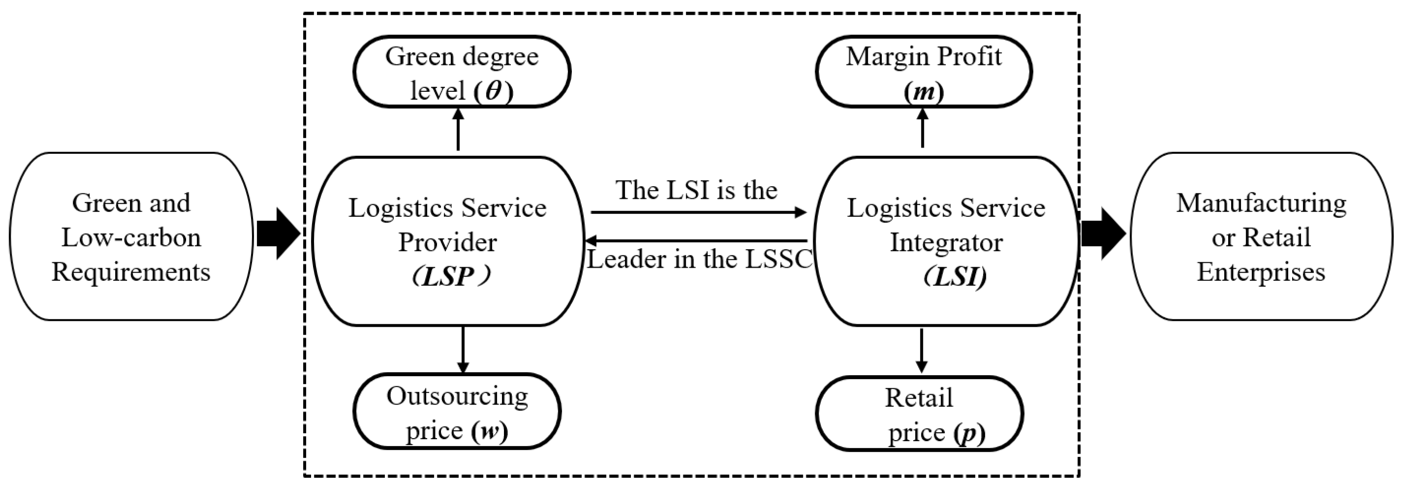
In practice, experts often use similar language, such as low cost, large market capacity, and sensitive demand change rate, to make empirical estimations. Furthermore, fuzzy theory can determine the relationship between experts’ fuzzy language and the triangular fuzzy number. Taking a green LSSC composed of a single LSI and a single LSP as the background, when providing services, the LSP must effectively address environmental problems, such as distribution, transportation, and warehousing. Hence, the LSP takes on greater environmental protection responsibility and bears more innovative research and development costs to provide an energy conservation and environmental protection green logistics service. Consequently, the structure of a two-stage green LSSC is as shown in Figure 1.

According to the above discussion, we explored the decision making in an LSSC composed of one LSI and one LSP under fuzzy environments with consideration of the influence of the environment, in which the LSI is the leader and the LSP is the follower. The LSP provides logistics service to the LSI with an outsourced price. Then, the LSI sends logistics services to the customers (manufacturing or retail enterprises) by integrating the LSP’s service quality to meet the demands of the customers.

In the process, an LSP with awareness of the environment provides specific feature services to its partners, thereby, using the greening level to measure the impact of the environment from the LSP. The decision variables for the LSI are the price and margin profit. For the LSP, the decision variables are the outsourcing price and the greening level. Respectively, different fuzzy expected value and chance-constrained programming models were established to analyze the Stackelberg game of a risk-neutral LSI and an LSP with different risk preferences; an LSI with different risk preferences and a risk-neutral LSP; and an LSI and LSP with the same risk preferences.

3.2. Model Assumptions

To build the game model for LSSC decision making, the following basic assumptions were considered in this paper:

Assumption 1.

Considering a perfectly competitive market environment, there is only one green service in the market. The LSP provides green logistics service to the LSI with outsourcing price w; then, the LSI sends them to the customers with price p, and p = (m + w). θ is the greening level of the green logistics service. The higher θ is, the more environmental the logistics service is, and θ > 0.

Assumption 2.

Following Jamali et al. [4] and Wang et al. [39], the logistics service demand q is comprehensively affected by the overall scale, price, and greening level under fuzzy environments.

$$\tilde{q}=\tilde{B}-\tilde{\beta }p+\tilde{\gamma }\theta$$

(1)

where $\tilde{B}$, $\tilde{\beta }$, and $\tilde{\gamma }$ are the independent non-negative fuzzy variables, and $\tilde{B}>0$, $\tilde{\beta }>0$, and $\tilde{\gamma }>0$. Moreover, there is $\tilde{\beta }>\tilde{\gamma }$, which means that the demand for the green service is more sensitive to its price than its green level. Additionally, we have $Pos\{p-\tilde{c}<0\}=0$ and $Pos\{\tilde{B}-\tilde{\beta }p+\tilde{\gamma }\theta <0\}=0$ which means that the possibilities of the event $\{p-\tilde{c}\}$ and $\{\tilde{B}-\tilde{\beta }p+\tilde{\gamma }\theta \}$ are all zero. This assumption is reasonable, in the case that most consumer environmental awareness is low, and the net surplus and the customer demand are nonnegative in the real world.

Assumption 3.

For environmental sustainability, more technological innovations should be involved in logistics services. An important factor of the LSP’s service is to decrease the adverse externalities of the environment. Hence, the LSP should bear the investment’s service cost. We assumed that the LSP’s investment in technological innovation is $c_p=\frac{1}{2}\tilde{\xi }{\theta }^2$, where $\tilde{\xi }$ is the greening innovation coefficient of logistics services. This quadratic service cost function has been widely used, including by Sun et al. [2] and Jamali et al. [4].

Assumption 4.

To ensure that the profits of the LSI and LSP are all positive, all parameters are assumed to be non-negative and to satisfy the following relationship: $\frac{{\tilde{\beta }}_{\alpha }^U{\tilde{\xi }}_{\alpha }^U}{{\left({\tilde{\gamma }}_{\alpha }^L\right)}^2}>1$, $\frac{{\tilde{\beta }}_{\alpha }^L{\tilde{\xi }}_{\alpha }^L}{{\left({\tilde{\gamma }}_{\alpha }^U\right)}^2}>1$, $\frac{E\left[\tilde{\beta }\right]E\left[\tilde{\xi }\right]}{{\left(E\left[\tilde{\gamma }\right]\right)}^2}>1$.

Assumption 5.

We assumed that the different risk preferences of the LSI and LSP refer to the different decision making attitudes when dealing with the risks of the green supply chain system, which can be divided into three risk preferences: neutral, pessimistic, and optimistic. Neutral decision makers are rational people who make rational decisions, and whose profit is expressed as the expected value. Pessimistic decision makers generally treat risks cautiously and take more conservative measures to deal with them, and their profit is expressed as ${\pi }_{\alpha }^L=inf\left\{r\right|Pos\{\pi \le r\}\ge \alpha \}$ and called α pessimistic value.

Optimistic decision makers generally pursue the concept of high risk and high return and prefer to earn higher returns and bear higher risk; their profit is expressed as ${\pi }_{\alpha }^U=sup\left\{r\right|Pos\{\pi \ge r\}\ge \alpha \}$ and called the α optimistic value.

Based on the problem description and the presented model assumptions, under the fuzzy environment, the profit functions for the LSP, LSI, and LSSC are obtained by Equations (2)–(4):

$${\tilde{\pi }}_P=\left(w-\tilde{c}\right)(\tilde{B}-\tilde{\beta }(\mathit{m}+\mathit{w})+\tilde{\gamma }\theta )-\frac{1}{2}\tilde{\xi }{\theta }^2$$

(2)

$${\tilde{\pi }}_I=m(\tilde{B}-\tilde{\beta }(\mathit{m}+\mathit{w})+\tilde{\gamma }\theta )$$

(3)

$${\tilde{\pi }}_{SC}=\left(\mathit{m}+\mathit{w}-\tilde{c}\right)(\tilde{B}-\tilde{\beta }(\mathit{m}+\mathit{w})+\tilde{\gamma }\theta )-\frac{1}{2}\tilde{\xi }{\theta }^2$$

(4)

4. The Model Building

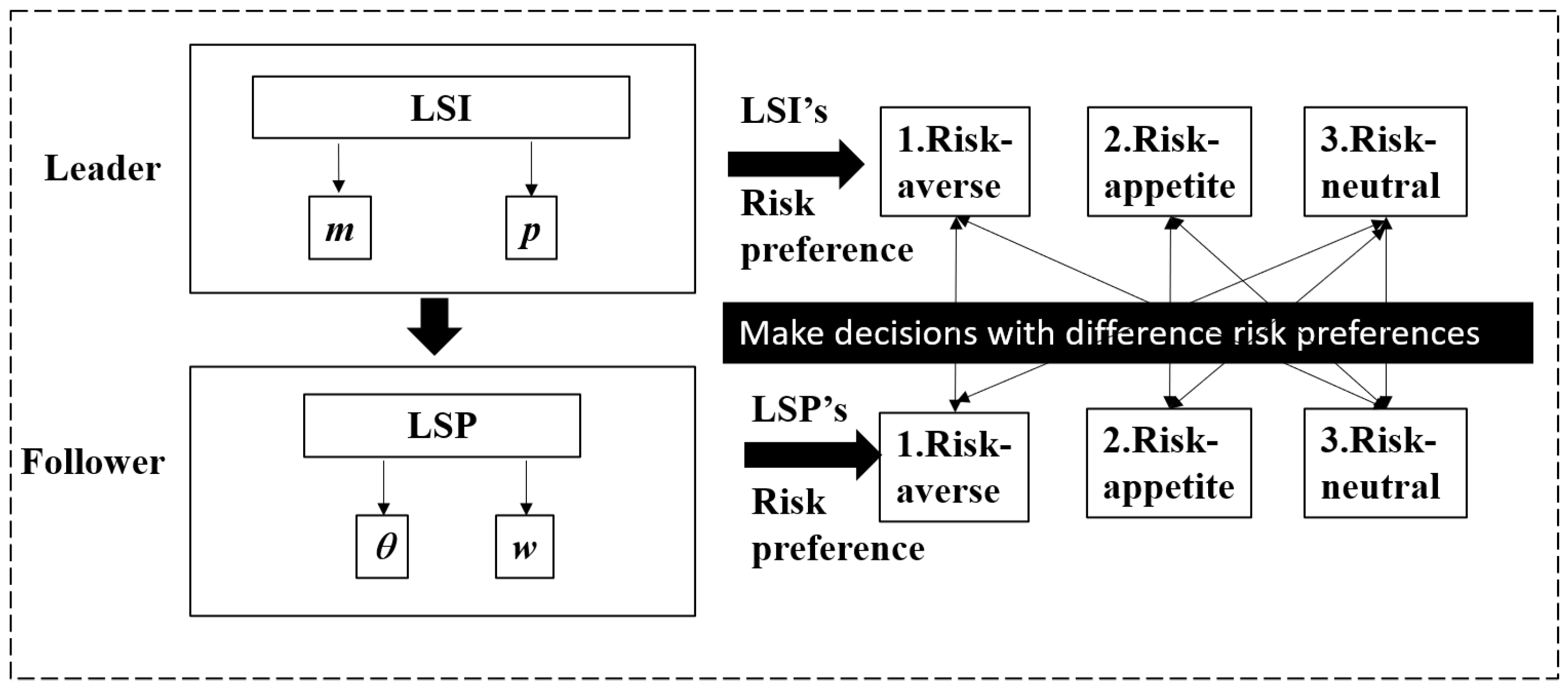
In this section, we assumed that the LSI and LSP present a Stackelberg game in the LSSC. The LSI is the leader, and it determines the profit margin of the green logistics service by using the respond function of the LSP. Then, the LSP acts as the follower, and it decides the greening level and outsourcing price of the logistics service. In similar studies [40,41], different risk preference behaviors of LSSC members were proposed by the fuzzy expected value model and the chance-constrained programming model. The decision making process of the LSP and LSI was simulated with the following three scenarios, as shown in Figure 2.

Scenario 1: A game between the risk-neutral LSI and LSP with different risk preferences. In this case, there are two-echelon LSSC models composed of a risk-neutral LSI and a risk averse or risk appetite LSP, namely, a pessimistic or optimistic LSP under a fuzzy decision environment, indexed by the subscripts NP and NO, respectively.

Scenarios 2: A game between the LSI with different risk preferences and a risk-neutral LSP. In this case, there are LSSC models composed of a risk averse or risk appetite LSI and a risk-neutral LSP under a fuzzy decision environment, indexed by the subscripts PN and ON, respectively.

Scenarios 3: A game between the LSI and LSP with the same risk preferences. In this case, both the LSI and LSP with risk-neutral, risk-averse, or risk appetite attitudes are explored in the LSSC models, indexed by the subscripts NN, PP, and OO, respectively.

For the different scenarios, we built different models. The optimal decisions of the LSP and the LSI were first investigated; the corresponding optimal outsourcing price and the optimal price of a green logistics service could then be estimated; and finally, the optimal greening level was determined. Taking all of these results into consideration, a comparison was conducted among the three scenarios.

4.1. A Risk-Neutral LSI and an LSP with Different Risk Preferencesl

In this scenario, there were two LSSC models composed of a risk-neutral LSI acting as the leader and a risk averse or risk appetite LSP acting as the follower under a fuzzy decision environment, and these can be called the pessimistic LSP decision model and the optimistic LSP decision model, respectively.

The risk-neutral LSI determines the profit margin of the green logistics service by using the respond function of the different risk preferences LSP. After this, the LSP decides the greening level and outsourcing price of the green logistics service. Based on the fuzzy chance-constrained programming model proposed by Liu et al. [40], the benefits of decision-makers can be maximized at a certain confidence level. Then, we can obtain the minimax and maximax chance-constrained programming for the LSSC.

4.1.1. The Pessimistic LSP Decision Model

In this section, the fuzzy LSSC used a risk-neutral LSI as the leader and a risk-averse pessimistic LSP as the follower, indexed by the subscript NP. The risk-neutral LSI determines the profit margin (m), and the risk-averse LSP decides the greening level ($\theta$) and outsourcing price (w) to maximize their profit. Hence, we can obtain the minimax chance-constrained programming for the LSSC.

$$\left\{\begin{array}{cc}\hfill & \underset{m}{\max }E\left[{\tilde{\pi }}_I\left(m,w^{*}\left(m\right),{\theta }^{*}\left(m\right)\right)\right]=E\left[m\left(\tilde{B}-\tilde{\beta }\left(m+w^{*}\left(m\right)\right)+\tilde{\gamma }{\theta }^{*}\left(m\right)\right)\right]\hfill \\ \hfill & s.t.\hfill \\ \hfill & P\mathrm{os}\left\{m\le 0\right\}=0\hfill \\ \hfill & w^{*},{\theta }^{*}=arg\underset{\left(w,\theta \right)}{\max }\underset{{\tilde{\pi }}_P}{\min }{\tilde{\pi }}_P\hfill \\ \hfill & \left\{\begin{array}{cc}\hfill & \underset{\left(w,\theta \right)}{\max }\underset{{\tilde{\pi }}_P}{\min }{\tilde{\pi }}_P\hfill \\ \hfill & s.t.\hfill \\ \hfill & P\mathrm{os}\left\{\left(w-\tilde{c}\right)\left(\tilde{B}-\tilde{\beta }\left(m+w\right)+\tilde{\gamma }\theta \right)-\frac{1}{2}\tilde{\xi }{\theta }^2\le {\tilde{\pi }}_P\right\}\ge \alpha \hfill \\ \hfill & P\mathrm{os}\left\{\tilde{B}-\tilde{\beta }\left(m+w\right)+\tilde{\gamma }\theta \le 0\right\}=0\hfill \\ \hfill & w\ge \tilde{c}\hfill \end{array}\right.\hfill \end{array}\right.$$

(5)

where $\alpha$ is a predetermined confidence level for the profit of the LSP and LSI. For each fixed feasible solution $(\mathit{w},\theta )$, $\min {\tilde{\pi }}_P$ is the minimum value that the LSP’s profit function ${\pi }_P(\mathit{w},\theta )$ obtains with the least possible $\alpha$, and $E\left[{\tilde{\pi }}_I\right]$ is the expected profit of the risk-neutral LSI. We formulated the following minimax chance-constrained programming model in which the risk-neutral LSI and the risk-averse LSP attempt to maximize their optimal expected and $\alpha$-pessimistic profit by selecting the best $(\mathit{w},\theta )$ and $\mathit{m}$ strategies, respectively [40,41].

It is clear that model (5) can be recast as model (6):

$$\left\{\begin{array}{cc}\hfill & \underset{m}{\max }E\left[{\tilde{\pi }}_I\left(m,w^{*}\left(m\right),{\theta }^{*}\left(m\right)\right)\right]=E\left[m\left(\tilde{B}-\tilde{\beta }\left(m+w^{*}\left(m\right)\right)+\tilde{\gamma }{\theta }^{*}\left(m\right)\right)\right]\hfill \\ \hfill & s.t.\hfill \\ \hfill & P\mathrm{os}\left\{m\le 0\right\}=0\hfill \\ \hfill & w^{*},{\theta }^{*}=arg\underset{\left(w,\theta \right)}{\max }{\left({\tilde{\pi }}_P\left(w,\theta \right)\right)}_{\alpha }^L\hfill \\ \hfill & \left\{\begin{array}{cc}\hfill & \underset{\left(w,\theta \right)}{\max }{\left({\tilde{\pi }}_P\left(w,\theta \right)\right)}_{\alpha }^L={\left(\left(w-\tilde{c}\right)\left(\tilde{B}-\tilde{\beta }\left(m+w\right)+\tilde{\gamma }\theta \right)-\frac{1}{2}\tilde{\xi }{\theta }^2\right)}_{\alpha }^L\hfill \\ \hfill & s.t.\hfill \\ \hfill & P\mathrm{os}\left\{\tilde{B}-\tilde{\beta }\left(m+w\right)+\tilde{\gamma }\theta \le 0\right\}=0\hfill \\ \hfill & w\ge \tilde{c}\hfill \end{array}\right.\hfill \end{array}\right.$$

(6)

Theorem 1.

Let $E\left[{\tilde{\pi }}_I\right]$, ${\left({\tilde{\pi }}_P(w,\theta )\right)}_{\alpha }^L$ be the expected profit of the risk-neutral LSI and α-pessimistic value of the risk-averse LSP’s profit, respectively. The profit margin textitm chosen by the LSI is given. If $Pos\{\frac{{\tilde{B}}_{\alpha }^L+({\tilde{c}}_{\alpha }^U-m){\tilde{\beta }}_{\alpha }^U)-{\tilde{c}}_{\alpha }^U{\left({\tilde{\gamma }}_{\alpha }^L\right)}^2}{2{\left(\tilde{\beta }\tilde{\xi }\right)}_{\alpha }^U-{\left({\tilde{\gamma }}_{\alpha }^L\right)}^2}\le \tilde{c}\}=0$, $\frac{{\tilde{\beta }}_{\alpha }^U{\tilde{\xi }}_{\alpha }^U}{{\left({\tilde{\gamma }}_{\alpha }^L\right)}^2}>\frac{1}{2}$ and $Pos\{m_{NP}^{*}\le 0\}=0$, then the optimal solutions ($m_{NP}^{*}$, ${\theta }_{NP}^{*}$, $w_{NP}^{*}$, $p_{NP}^{*}$) of the fuzzy LSSC are:

$$\begin{gathered} \begin{array}{cc}{m_{NP}}^{*}=& \frac{{\tilde{\gamma }}_{\alpha }^{L}E\left[\tilde{\gamma }\right]({\tilde{B}}_{\alpha }^L-{\left(\tilde{\beta }\tilde{c}\right)}_{\alpha }^U)-\left({\tilde{\gamma }}_{\alpha }^L\right){}^2(E\left[\tilde{B}\right]-E\left[\tilde{\beta }\right]{\tilde{c}}_{\alpha }^U) \\ +{\tilde{\xi }}_{\alpha }^U((2E\left[\tilde{B}\right]-E\left[\tilde{\beta }\right]{\tilde{c}}_{\alpha }^U){\tilde{\beta }}_{\alpha }^U-E\left[\tilde{\beta }\right]{\tilde{B}}_{\alpha }^L)}{2E\left[\tilde{\beta }\right]{\left(\tilde{\beta }\tilde{\xi }\right)}_{\alpha }^U+2E\left[\tilde{\gamma }\right]{\tilde{\beta }}_{\alpha }^U{\tilde{\gamma }}_{\alpha }^L-E\left[\tilde{\beta }\right])\left({\tilde{\gamma }}_{\alpha }^L\right){}^2}\end{array} \end{gathered}$$

(7)

$$\begin{gathered} \begin{array}{c}{\theta }_{NP}^{*}=\frac{({\tilde{\gamma }}_{\alpha }^L{)}^3(2E\left[\tilde{\beta }\right]{\tilde{B}}_{\alpha }^L-{\tilde{\beta }}_{\alpha }^U(E\left[\tilde{B}\right]+E\left[\tilde{\beta }\right]{\tilde{c}}_{\alpha }^U)) \\ -({\tilde{\gamma }}_{\alpha }^L{)}^{2}E\left[\tilde{\gamma }\right]{\tilde{\beta }}_{\alpha }^U({\tilde{B}}_{\alpha }^L-{\tilde{c}}_{\alpha }^U{\tilde{\beta }}_{\alpha }^U) \\ -{\tilde{\gamma }}_{\alpha }^L{\left(\tilde{c}\tilde{\beta }\right)}_{\alpha }^U(3E\left[\tilde{\beta }\right]B_{\alpha }^L-{\tilde{\beta }}_{\alpha }^U(2E\left[\tilde{B}\right]+E\left[\tilde{\beta }\right]{\tilde{c}}_{\alpha }^U))}{2(2{\left(\tilde{\beta }\tilde{\xi }\right)}_{\alpha }^U-{({\tilde{\gamma }}_{\alpha }^L)}^2)(E\left[\tilde{\beta }\right]{({\tilde{\gamma }}_{\alpha }^L)}^2-{\tilde{\beta }}_{\alpha }^U(E\left[\tilde{\gamma }\right]{\tilde{\gamma }}_{\alpha }^L+E\left[\tilde{\beta }\right]{\tilde{\xi }}_{\alpha }^U))}\end{array} \end{gathered}$$

(8)

$$\begin{gathered} \begin{array}{c}{w}_{NP}^{*}=\frac{E\left[\tilde{B}\right]{\left(\tilde{\beta }\tilde{\xi }\right)}_{\alpha }^U(2{\left(\tilde{\beta }\tilde{\xi }\right)}_{\alpha }^U-({\tilde{\gamma }}_{\alpha }^L{)}^2)+{\tilde{B}}_{\alpha }^L{\tilde{\xi }}_{\alpha }^U(2E\left[\tilde{\beta }\right]({\tilde{\gamma }}_{\alpha }^L{)}^2-{\tilde{\beta }}_{\alpha }^U(E\left[\tilde{\gamma }\right]{\tilde{\gamma }}_{\alpha }^L+3E\left[\tilde{\beta }\right]{\tilde{\xi }}_{\alpha }^U)) \\ -{\tilde{c}}_{\alpha }^U(3{\left(\tilde{\beta }\tilde{\xi }\right)}_{\alpha }^U-2({\tilde{\gamma }}_{\alpha }^L{)}^2)({\tilde{\beta }}_{\alpha }^U(E\left[\tilde{\gamma }\right]{\tilde{\gamma }}_{\alpha }^L+E\left[\tilde{\beta }\right]{\tilde{\xi }}_{\alpha }^U)-E\left[\tilde{\beta }\right]({\tilde{\gamma }}_{\alpha }^L{)}^2)}{2(2{\left(\tilde{\beta }\tilde{\xi }\right)}_{\alpha }^U-{({\tilde{\gamma }}_{\alpha }^L)}^2)(E\left[\tilde{\beta }\right]{({\tilde{\gamma }}_{\alpha }^L)}^2-{\tilde{\beta }}_{\alpha }^U(E\left[\tilde{\gamma }\right]{\tilde{\gamma }}_{\alpha }^L+E\left[\tilde{\beta }\right]{\tilde{\xi }}_{\alpha }^U))}\end{array} \end{gathered}$$

(9)

$$\begin{gathered} \begin{array}{c}{p}_{NP}^{*}=\frac{({\tilde{\beta }}_{\alpha }^U{\tilde{\xi }}_{\alpha }^U-{\left({\tilde{\gamma }}_{\alpha }^L\right)}^2)({\tilde{\gamma }}_{\alpha }^L((E\left[\tilde{B}\right]+E\left[\tilde{\beta }\right]{\tilde{c}}_{\alpha }^U){\tilde{\gamma }}_{\alpha }^L-E\left[\tilde{\gamma }\right]{\tilde{c}}_{\alpha }^U{\tilde{\beta }}_{\alpha }^U)-(2E\left[\tilde{B}\right]+E\left[\tilde{\beta }\right]{\tilde{c}}_{\alpha }^U){\tilde{\beta }}_{\alpha }^U{\tilde{\xi }}_{\alpha }^U) \\ -{\tilde{B}}_{\alpha }^L({\tilde{\gamma }}_{\alpha }^L{\tilde{\xi }}_{\alpha }^U(3E\left[\tilde{\gamma }\right]{\tilde{\beta }}_{\alpha }^U-E\left[\tilde{\beta }\right]{\tilde{\gamma }}_{\alpha }^L)+E\left[\tilde{\beta }\right]{\tilde{\beta }}_{\alpha }^U{{(\tilde{\xi }}_{\alpha }^U)}^2-E\left[\tilde{\gamma }\right]{{(\tilde{\gamma }}_{\alpha }^L)}^3)}{2(2{\left(\tilde{\beta }\tilde{\xi }\right)}_{\alpha }^U-{({\tilde{\gamma }}_{\alpha }^L)}^2][E\left[\tilde{\beta }\right]{({\tilde{\gamma }}_{\alpha }^L)}^2-{\tilde{\beta }}_{\alpha }^U(E\left[\tilde{\gamma }\right]{\tilde{\gamma }}_{\alpha }^L+E\left[\tilde{\beta }\right]{\tilde{\xi }}_{\alpha }^U))}\end{array} \end{gathered}$$

(10)

Proof. 

According to Equations (2) and (3), we can obtain the expected profit of the risk-neutral LSI $E\left[{\tilde{\pi }}_I\right]$ and the $\alpha$-pessimistic value of the risk-averse LSP’s profit, respectively.

$$\begin{array}{c}\hfill E\left[{\tilde{\pi }}_I\right]=\frac{1}{2}{\int }_0^1{\left(m(\tilde{B}-\tilde{\beta }p+\tilde{\gamma }\theta )\right)}_{\alpha }^L+\frac{1}{2}{\int }_0^1{\left(m(\tilde{B}-\tilde{\beta }p+\tilde{\gamma }\theta )\right)}_{\alpha }^U\\ \hfill =-m^{2}E\left[\tilde{\beta }\right]+mE\left[\tilde{B}\right]-mwE\left[\tilde{\beta }\right]+m\theta E\left[\tilde{\gamma }\right]\end{array}$$

(11)

$$\begin{array}{c}\hfill {\left({\tilde{\pi }}_P(w,\theta )\right)}_{\alpha }^L=(w-{\tilde{c}}_{\alpha }^U)({\tilde{B}}_{\alpha }^L-{\tilde{\beta }}_{\alpha }^U(m+w)+{\tilde{\gamma }}_{\alpha }^L\theta )-\frac{1}{2}{\tilde{\xi }}_{\alpha }^U{\theta }^2\\ \hfill =-{\tilde{\beta }}_{\alpha }^U{w}^2+w{\tilde{B}}_{\alpha }^L-wm{\tilde{\beta }}_{\alpha }^U+w\theta {\tilde{\gamma }}_{\alpha }^L+m{\tilde{c}}_{\alpha }^U{\tilde{\beta }}_{\alpha }^U+w{\tilde{c}}_{\alpha }^U{\tilde{\beta }}_{\alpha }^U-{\tilde{c}}_{\alpha }^U{\tilde{\gamma }}_{\alpha }^L\theta -\frac{1}{2}{\tilde{\xi }}_{\alpha }^U{\theta }^2-{\tilde{c}}_{\alpha }^U{\tilde{B}}_{\alpha }^L\end{array}$$

(12)

From Equation (10), the first-order derivatives of ${\left({\tilde{\pi }}_P(w,\theta )\right)}_{\alpha }^L$ with respect to w and $\theta$ can be obtained:

$$\frac{\partial {\left({\tilde{\pi }}_P(w,\theta )\right)}_{\alpha }^L}{\partial w}=-{\tilde{\beta }}_{\alpha }^{U}w+{\tilde{B}}_{\alpha }^L-m{\tilde{\beta }}_{\alpha }^U+\theta {\tilde{\gamma }}_{\alpha }^L+{\tilde{c}}_{\alpha }^U{\tilde{\beta }}_{\alpha }^U$$

(13)

$$\frac{\partial {\left({\tilde{\pi }}_P(w,\theta )\right)}_{\alpha }^L}{\partial \theta }=w{\tilde{\gamma }}_{\alpha }^L-{\tilde{c}}_{\alpha }^U{\tilde{\gamma }}_{\alpha }^L-{\tilde{\xi }}_{\alpha }^U\theta$$

(14)

Therefore, the Hesse matrix of the ${\left({\tilde{\pi }}_P(w,\theta )\right)}_{\alpha }^L$ with respect to w and $\theta$ is $H=\left|\begin{array}{cc}-2{\tilde{\beta }}_{\alpha }^U& {\tilde{\gamma }}_{\alpha }^L\\ {\tilde{\gamma }}_{\alpha }^L& -{\tilde{\xi }}_{\alpha }^U\end{array}\right|$. In fact, the Hesse matrix of the ${\left({\tilde{\pi }}_P(w,\theta )\right)}_{\alpha }^L$ is negative definite, as $2{\tilde{\beta }}_{\alpha }^U{\tilde{\xi }}_{\alpha }^U-{\left({\tilde{\gamma }}_{\alpha }^L\right)}^2>0$, $H=\left|\begin{array}{cc}-2{\tilde{\beta }}_{\alpha }^U& {\tilde{\gamma }}_{\alpha }^L\\ {\tilde{\gamma }}_{\alpha }^L& -{\tilde{\xi }}_{\alpha }^U\end{array}\right|>0$ and $\tilde{\beta }$, $\tilde{\gamma }$, $\tilde{\xi }$ are positive fuzzy variables. Consequently, ${\left({\tilde{\pi }}_P(w,\theta )\right)}_{\alpha }^L$ is jointly concave in $\mathit{w}$ and $\theta$. Therefore, we can obtain the optimal response functions ${\mathit{w}}^{*}\left(m\right)$ and ${\theta }^{*}\left(m\right)$ of LSP by solving $\frac{\partial {\left({\tilde{\pi }}_P(w,\theta )\right)}_{\alpha }^L}{\partial w}=0$ and $\frac{\partial {\left({\tilde{\pi }}_P(w,\theta )\right)}_{\alpha }^L}{\partial \theta }=0$, which provides (15) and (16).

$$w_{NP}^{*}\left(m\right)=\frac{({\tilde{B}}_{\alpha }^L+({\tilde{c}}_{\alpha }^U-m){\tilde{\beta }}_{\alpha }^U){\tilde{\xi }}_{\alpha }^U-{\tilde{c}}_{\alpha }^U{\left({\tilde{\gamma }}_{\alpha }^L\right)}^2}{2{\tilde{\beta }}_{\alpha }^U{\tilde{\xi }}_{\alpha }^U-{\left({\tilde{\gamma }}_{\alpha }^L\right)}^2}$$

(15)

$${\theta }_{NP}^{*}\left(m\right)=\frac{({\tilde{B}}_{\alpha }^L-{\left(\tilde{c}\tilde{\beta }\right)}_{\alpha }^U-m{\tilde{\beta }}_{\alpha }^U){\tilde{\gamma }}_{\alpha }^L}{2{\tilde{\beta }}_{\alpha }^U{\tilde{\xi }}_{\alpha }^U-{\left({\tilde{\gamma }}_{\alpha }^L\right)}^2}$$

(16)

Substituting $w_{NP}^{*}\left(m\right)$ and ${\theta }_{NP}^{*}\left(m\right)$ in Equations (15) and (16) into Equation (3), we can obtain:

$$\begin{array}{c}\hfill E\left[{\tilde{\pi }}_I\right]=-m^{2}E\left[\tilde{\beta }\right]-mE\left[\tilde{\beta }\right]\frac{({\tilde{B}}_{\alpha }^L+({\tilde{c}}_{\alpha }^U-m){\tilde{\beta }}_{\alpha }^U)-{\tilde{c}}_{\alpha }^U{({\tilde{\gamma }}_{\alpha }^L)}^2}{2\tilde{\beta }{\tilde{\xi }}_{\alpha }^U-{({\tilde{\gamma }}_{\alpha }^L)}^2}\\ \hfill +mE\left[\tilde{B}\right]+mE\left[\tilde{\gamma }\right]\frac{({\tilde{B}}_{\alpha }^L+\tilde{\beta }{\tilde{c}}_{\alpha }^U-m{\tilde{\beta }}_{\alpha }^U){\tilde{\gamma }}_{\alpha }^L}{2\tilde{\beta }{\tilde{\xi }}_{\alpha }^U-{({\tilde{\gamma }}_{\alpha }^L)}^2}\end{array}$$

(17)

Thus, the first and second-order derivatives of $E\left[{\tilde{\pi }}_I\right]$ with respect to m can be obtained:

$$\begin{gathered} \begin{array}{c}\frac{\partial E\left[{\tilde{\pi }}_I\left(m\right)\right]}{\partial m}=\frac{-{\tilde{\gamma }}_{\alpha }^L(E\left[\tilde{B}\right]{\tilde{\gamma }}_{\alpha }^L-{\tilde{B}}_{\alpha }^{L}E\left[\tilde{\gamma }\right]+\left(2m+{\tilde{c}}_{\alpha }^U\right)(E\left[\tilde{\gamma }\right]{\tilde{\beta }}_{\alpha }^U-E\left[\tilde{\beta }\right]{\tilde{\gamma }}_{\alpha }^L)) \\ -{\tilde{\xi }}_{\alpha }^U({\tilde{B}}_{\alpha }^{L}E\left[\tilde{\beta }\right]+{\tilde{\beta }}_{\alpha }^U(2mE\left[\tilde{\beta }\right]-2E\left[\tilde{B}\right]+E\left[\tilde{\beta }\right]{\tilde{c}}_{\alpha }^U))}{2{\tilde{\beta }}_{\alpha }^U{\tilde{\xi }}_{\alpha }^U-{\left({\tilde{\gamma }}_{\alpha }^L\right)}^2}\end{array} \end{gathered}$$

(18)

$$\begin{array}{c}\frac{{\partial }^{2}E\left[{\tilde{\pi }}_I\left(m\right)\right]}{\partial m^2}=\frac{-2E\left[\tilde{\beta }\right]{\tilde{\beta }}_{\alpha }^U{\tilde{\xi }}_{\alpha }^U-2(E\left[\tilde{\gamma }\right]{\tilde{\beta }}_{\alpha }^U-{\tilde{\gamma }}_{\alpha }^{L}E\left[\tilde{\beta }\right])}{2{\tilde{\beta }}_{\alpha }^U{\tilde{\xi }}_{\alpha }^U-{\left({\tilde{\gamma }}_{\alpha }^L\right)}^2}\end{array}$$

(19)

$E\left[{\tilde{\pi }}_I\left(m\right)\right]$ is a concave function in m, as $E\left[\tilde{\gamma }\right]>{\tilde{\gamma }}_{\alpha }^L$, ${\tilde{\beta }}_{\alpha }^U>E\left[\tilde{\beta }\right]$, $2{\tilde{\beta }}_{\alpha }^U{\tilde{\xi }}_{\alpha }^U-{\left({\tilde{\gamma }}_{\alpha }^L\right)}^2>0$, and all of the fuzzy variables are positive. The optimal margin profit of the risk-neutral LSI can be attained by solving $\frac{\partial E\left[{\tilde{\pi }}_I\left(m\right)\right]}{\partial m}=0$, which are shown in (7).

Then, substituting $m_{NP}^{*}$ into Equations (15) and (16), we can obtain the optimal ${\theta }_{NP}^{*}$ and $w_{NP}^{*}$, which are shown in (8) and (9) for the LSCC under the NP scenario. Combining Equations (7) and (9) into $m_{NP}^{*}+w_{NP}^{*}=p_{NP}^{*}$ easily yields the optimal price $p_{NP}^{*}$ of the LSI.

Thus, the proof of Theorem 1 is complete. □

4.1.2. The Optimistic LSP Decision Model

In this section, a risk-neutral LSI acts as the leader, and an optimistic risk appetite LSP acts as the follower under a fuzzy decision environment, indexed by the subscript NO. The risk-neutral LSI determines the profit margin (m), and the optimistic LSP decides the greening level $\left(\theta \right)$ and outsourcing price (w) to maximize their profit. The decision making model is as follows:

$$\left\{\begin{array}{cc}\hfill & \underset{m}{\max }E\left[{\tilde{\pi }}_I\left(m,w^{*}\left(m\right),{\theta }^{*}\left(m\right)\right)\right]=E\left[m\left(\tilde{B}-\tilde{\beta }\left(m+w^{*}\left(m\right)\right)+\tilde{\gamma }{\theta }^{*}\left(m\right)\right)\right]\hfill \\ \hfill & s.t.\hfill \\ \hfill & P\mathrm{os}\left\{m\le 0\right\}=0\hfill \\ \hfill & w^{*},{\theta }^{*}=arg\underset{\left(w,\theta \right)}{\max }{\tilde{\pi }}_P\hfill \\ \hfill & \left\{\begin{array}{cc}\hfill & \underset{\left(w,\theta \right)}{\max }{\tilde{\pi }}_P\hfill \\ \hfill & s.t.\hfill \\ \hfill & P\mathrm{os}\left\{\left(w-\tilde{c}\right)\left(\tilde{B}-\tilde{\beta }\left(m+w\right)+\tilde{\gamma }\theta \right)-\frac{1}{2}\tilde{\xi }{\theta }^2\ge {\tilde{\pi }}_P\right\}\ge \alpha \hfill \\ \hfill & P\mathrm{os}\left\{\tilde{B}-\tilde{\beta }\left(m+w\right)+\tilde{\gamma }\theta \le 0\right\}=0\hfill \\ \hfill & w\ge \tilde{c}\hfill \end{array}\right.\hfill \end{array}\right.$$

(20)

where $\alpha$ is a predetermined confidence level for the profit of the LSP and LSI. For each given feasible solution $(\mathit{w},\theta )$, $\max {\tilde{\pi }}_P$ is the maximum value that the optimistic LSP’s profit function ${\tilde{\pi }}_P(\mathit{w},\theta )$ obtains with least possible $\alpha$, and $E\left[{\tilde{\pi }}_I\right]$ is the expected profit of the risk-neutral LSI. We formulated the following maximax chance-constrained programming model in which a risk-neutral LSI and a risk appetite LSP atempt to maximize their optimal expected and $\alpha$-optimistic profit by selecting the bestm and $(\mathit{w},\theta )$ strategies, respectively.

It is clear that model (20) can be reformulated as model (21):

$$\left\{\begin{array}{cc}& \underset{m}{\max }E\left[{\tilde{\pi }}_I\left(m,w^{*}\left(m\right),{\theta }^{*}\left(m\right)\right)\right]=E\left[m\left(\tilde{B}-\tilde{\beta }\left(m+w^{*}\left(m\right)\right)+\tilde{\gamma }{\theta }^{*}\left(m\right)\right)\right]\hfill \\ & s.t.\hfill \\ & P\mathrm{os}\left\{m\le 0\right\}=0\hfill \\ & w^{*},{\theta }^{*}=arg\underset{\left(w,\theta \right)}{\max }{\left({\tilde{\pi }}_P\left(w,\theta \right)\right)}_{\alpha }^U\hfill \\ & \left\{\begin{array}{cc}& \underset{\left(w,\theta \right)}{\max }{\left({\tilde{\pi }}_P\left(w,\theta \right)\right)}_{\alpha }^U={\left(\left(w-\tilde{c}\right)\left(\tilde{B}-\tilde{\beta }\left(m+w\right)+\tilde{\gamma }\theta \right)-\frac{1}{2}\tilde{\xi }{\theta }^2\right)}_{\alpha }^U\hfill \\ & s.t.\hfill \\ & P\mathrm{os}\left\{\tilde{B}-\tilde{\beta }\left(m+w\right)+\tilde{\gamma }\theta \le 0\right\}=0\hfill \\ & w\ge \tilde{c}\hfill \end{array}\right.\hfill \end{array}\right.$$

(21)

Theorem 2.

Let $E\left[{\tilde{\pi }}_I(m,w^{*}\left(m\right),{\theta }^{*}\left(m\right))\right]$ and ${\left({\tilde{\pi }}_P(w,\theta )\right)}_{\alpha }^U$ be the expected profit of the risk-neutral LSI and the α-optimistic value of the risk appetite LSP’s profit, respectively. The profit margin m chosen by LSI is given. If $Pos\{\frac{{\tilde{B}}_{\alpha }^U+({\tilde{c}}_{\alpha }^L-m){\tilde{\beta }}_{\alpha }^L)-{\tilde{c}}_{\alpha }^L{\left({\tilde{\gamma }}_{\alpha }^U\right)}^2}{2{\left(\tilde{\beta }\tilde{\xi }\right)}_{\alpha }^L-{\left({\tilde{\gamma }}_{\alpha }^U\right)}^2}\le \tilde{c}\}=0$, $2{\tilde{\beta }}_{\alpha }^U{\tilde{\xi }}_{\alpha }^U-{\left({\tilde{\gamma }}_{\alpha }^L\right)}^2>0$ and $Pos\{m_{NP}^{*}\le 0\}=0$, then the optimal solutions of the fuzzy LSSC are:

$$\begin{gathered} \begin{array}{c}{m}_{NO}^{*}=\frac{{\tilde{\gamma }}_{\alpha }^{U}E\left[\tilde{\gamma }\right]({\tilde{B}}_{\alpha }^U-{\left(\tilde{\beta }\tilde{c}\right)}_{\alpha }^L)-\left({\tilde{\gamma }}_{\alpha }^U\right){}^2(E\left[\tilde{B}\right]-E\left[\tilde{\beta }\right]{\tilde{c}}_{\alpha }^L) \\ +{\tilde{\xi }}_{\alpha }^L((2E\left[\tilde{B}\right]-E\left[\tilde{\beta }\right]c_{\alpha }^L){\tilde{\beta }}_{\alpha }^L-E\left[\tilde{\beta }\right]{\tilde{B}}_{\alpha }^U)}{2E\left[\tilde{\beta }\right]{\left(\tilde{\beta }\tilde{\xi }\right)}_{\alpha }^L+E\left[\tilde{\gamma }\right]{\tilde{\beta }}_{\alpha }^L{\tilde{\gamma }}_{\alpha }^U-E\left[\tilde{\beta }\right])\left({\tilde{\gamma }}_{\alpha }^U\right){}^2}\end{array} \end{gathered}$$

(22)

$$\begin{gathered} \begin{array}{c}{\theta }_{NO}^{*}=\frac{({\tilde{\gamma }}_{\alpha }^U{)}^3(2E\left[\tilde{\beta }\right]{\tilde{B}}_{\alpha }^U-{\tilde{\beta }}_{\alpha }^L(E\left[\tilde{B}\right]+E\left[\tilde{\beta }\right]{\tilde{c}}_{\alpha }^L))- \\ ({\tilde{\gamma }}_{\alpha }^U{)}^{2}E\left[\tilde{\gamma }\right]{\tilde{\beta }}_{\alpha }^L({\tilde{B}}_{\alpha }^U-{\tilde{c}}_{\alpha }^L{\tilde{\beta }}_{\alpha }^L)-{\tilde{\gamma }}_{\alpha }^U{\left(\tilde{c}\tilde{\beta }\right)}_{\alpha }^L(3E\left[\beta \right]B_{\alpha }^U-{\tilde{\beta }}_{\alpha }^L(2E\left[\tilde{B}\right]+E\left[\tilde{\beta }\right]{\tilde{c}}_{\alpha }^L))}{2(2{\left(\tilde{\beta }\tilde{\xi }\right)}_{\alpha }^L-{({\gamma }_{\alpha }^U)}^2][E\left[\beta \right]{({\gamma }_{\alpha }^U)}^2-{\beta }_{\alpha }^L(E\left[\gamma \right]{\gamma }_{\alpha }^U+E\left[\beta \right]{\xi }_{\alpha }^L))}\end{array} \end{gathered}$$

(23)

$$\begin{gathered} \begin{array}{c}{w}_{NO}^{*}=\frac{E\left[\tilde{B}\right]{\left(\tilde{\beta }\tilde{\xi }\right)}_{\alpha }^L[2\tilde{\beta }{\tilde{\xi }}_{\alpha }^L-({\tilde{\gamma }}_{\alpha }^U{)}^2]+{\tilde{B}}_{\alpha }^U{\tilde{\xi }}_{\alpha }^L[2E\left[\tilde{\beta }\right]({\tilde{\gamma }}_{\alpha }^U{)}^2-{\tilde{\beta }}_{\alpha }^L(E\left[\tilde{\gamma }\right]{\tilde{\gamma }}_{\alpha }^U+3E\left[\tilde{\beta }\right]{\tilde{\xi }}_{\alpha }^L)] \\ -{\tilde{c}}_{\alpha }^L(3\tilde{\beta }{\tilde{\xi }}_{\alpha }^L-2({\tilde{\gamma }}_{\alpha }^U{)}^2)({\tilde{\beta }}_{\alpha }^L(E\left[\tilde{\gamma }\right]{\tilde{\gamma }}_{\alpha }^U+E\left[\tilde{\beta }\right]{\tilde{\xi }}_{\alpha }^L)-E\left[\tilde{\beta }\right]({\tilde{\gamma }}_{\alpha }^U{)}^2)}{2(2{\left(\tilde{\beta }\tilde{\xi }\right)}_{\alpha }^L-{({\tilde{\gamma }}_{\alpha }^U)}^2)(E\left[\tilde{\beta }\right]{({\tilde{\gamma }}_{\alpha }^U)}^2-{\tilde{\beta }}_{\alpha }^L(E\left[\tilde{\gamma }\right]{\tilde{\gamma }}_{\alpha }^U+E\left[\tilde{\beta }\right]{\tilde{\xi }}_{\alpha }^L))}\end{array} \end{gathered}$$

(24)

$$\begin{gathered} \begin{array}{c}{p}_{NO}^{*}=\frac{({\tilde{\beta }}_{\alpha }^L{\tilde{\xi }}_{\alpha }^L-{\left({\tilde{\gamma }}_{\alpha }^U\right)}^2)({\tilde{\gamma }}_{\alpha }^U((E\left[\tilde{B}\right]+E\left[\tilde{\beta }\right]{\tilde{c}}_{\alpha }^L){\tilde{\gamma }}_{\alpha }^U-E\left[\tilde{\gamma }\right]{\tilde{c}}_{\alpha }^L{\tilde{\beta }}_{\alpha }^L)-(2E\left[\tilde{B}\right]+E\left[\tilde{\beta }\right]{\tilde{c}}_{\alpha }^L){\tilde{\beta }}_{\alpha }^L{\tilde{\xi }}_{\alpha }^L) \\ -{\tilde{B}}_{\alpha }^L({\tilde{\gamma }}_{\alpha }^U{\tilde{\xi }}_{\alpha }^L(3E\left[\tilde{\gamma }\right]{\tilde{\beta }}_{\alpha }^L-E\left[\tilde{\beta }\right]{\tilde{\gamma }}_{\alpha }^U)+E\left[\tilde{\beta }\right]{\tilde{\beta }}_{\alpha }^L{{(\tilde{\xi }}_{\alpha }^L)}^2-E\left[\tilde{\gamma }\right]{{(\tilde{\gamma }}_{\alpha }^U)}^3)}{2(2{\left(\tilde{\beta }\tilde{\xi }\right)}_{\alpha }^L-{({\tilde{\gamma }}_{\alpha }^U)}^2][E\left[\tilde{\beta }\right]{({\tilde{\gamma }}_{\alpha }^U)}^2-{\tilde{\beta }}_{\alpha }^L(E\left[\tilde{\gamma }\right]{\tilde{\gamma }}_{\alpha }^U+E\left[\tilde{\beta }t\right]{\tilde{\xi }}_{\alpha }^L))}\end{array} \end{gathered}$$

(25)

Proof. 

We can obtain the $\alpha$-optimistic value of the risk appetite LSP’s profit by:

$$\begin{array}{c}\hfill {\left({\tilde{\pi }}_P(w,\theta )\right)}_{\alpha }^U=(w-{\tilde{c}}_{\alpha }^L)({\tilde{B}}_{\alpha }^U-{\tilde{\beta }}_{\alpha }^L(m+w)+{\tilde{\gamma }}_{\alpha }^U\theta )-\frac{1}{2}{\tilde{\xi }}_{\alpha }^L{\theta }^2\\ \hfill =-{\tilde{\beta }}_{\alpha }^L{w}^2+w{\tilde{B}}_{\alpha }^U-wm{\tilde{\beta }}_{\alpha }^L+w\theta {\tilde{\gamma }}_{\alpha }^U+m{\tilde{c}}_{\alpha }^L{\tilde{\beta }}_{\alpha }^L+w{\tilde{c}}_{\alpha }^L{\tilde{\beta }}_{\alpha }^L-{\tilde{c}}_{\alpha }^L{\tilde{\gamma }}_{\alpha }^U\theta --\frac{1}{2}{\tilde{\xi }}_{\alpha }^L{\theta }^2-{\tilde{c}}_{\alpha }^L{\tilde{B}}_{\alpha }^U\end{array}$$

(26)

From Equation (26), the first-order derivatives of ${\left({\tilde{\pi }}_P(w,\theta )\right)}_{\alpha }^U$ with respect to $\mathit{w}$ and $\theta$ can be obtained. Then, similar to the Theorem 1 ${\left({\tilde{\pi }}_P(w,\theta )\right)}_{\alpha }^U$ is jointly concave in $\mathit{w}$ and $\theta$. Therefore, we can obtain the optimal response functions ${\mathit{w}}_{\mathit{NO}}^{*}\left(\mathit{m}\right)$ and ${\theta }_{\mathit{NO}}^{*}\left(\mathit{m}\right)$ of the risk appetite LSP by solving $\frac{{\left({\tilde{\pi }}_P(w,\theta )\right)}_{\alpha }^U}{\partial \mathit{w}}=0$ and $\frac{{\left({\tilde{\pi }}_P(w,\theta )\right)}_{\alpha }^U}{\partial \theta }=0$, which provides (27) and (28).

$$w_{NO}^{*}\left(m\right)=\frac{({\tilde{B}}_{\alpha }^U+({\tilde{c}}_{\alpha }^L-m){\tilde{\beta }}_{\alpha }^L)-{\tilde{c}}_{\alpha }^L{\left({\tilde{\gamma }}_{\alpha }^U\right)}^2}{2{\left(\tilde{\beta }\tilde{\xi }\right)}_{\alpha }^L-{\left({\tilde{\gamma }}_{\alpha }^U\right)}^2}$$

(27)

$$\begin{array}{c}\hfill {\left({\tilde{\pi }}_P(w,\theta )\right)}_{\alpha }^U=(w-{\tilde{c}}_{\alpha }^L)({\tilde{B}}_{\alpha }^U-{\tilde{\beta }}_{\alpha }^L(m+w)+{\tilde{\gamma }}_{\alpha }^U\theta )-\frac{1}{2}{\tilde{\xi }}_{\alpha }^L{\theta }^2\\ \hfill =-{\tilde{\beta }}_{\alpha }^L{w}^2+w{\tilde{B}}_{\alpha }^U-wm{\tilde{\beta }}_{\alpha }^L+w\theta {\tilde{\gamma }}_{\alpha }^U+m{\tilde{c}}_{\alpha }^L{\tilde{\beta }}_{\alpha }^L+w{\tilde{c}}_{\alpha }^L{\tilde{\beta }}_{\alpha }^L-{\tilde{c}}_{\alpha }^L{\tilde{\gamma }}_{\alpha }^U\theta --\frac{1}{2}{\tilde{\xi }}_{\alpha }^L{\theta }^2-{\tilde{c}}_{\alpha }^L{\tilde{B}}_{\alpha }^U\end{array}$$

(28)

Then, substituting $w_{NO}^{*}\left(m\right)$ and ${\theta }_{NO}^{*}\left(m\right)$ into Equation (3), we can obtain the expected profit of the risk-neutral LSI$E\left[{\tilde{\pi }}_I(m,w_{NO}^{*}\left(m\right),{\theta }_{NO}^{*}\left(m\right))\right]$.

Thus, the first and second order derivatives of $E\left[{\tilde{\pi }}_I(m,w_{NO}^{*}\left(m\right),{\theta }_{NO}^{*}\left(m\right))\right]$ with respect to m can be obtained, Similar to the Theorem 1, $E\left[{\tilde{\pi }}_I(m,w_{NO}^{*}\left(m\right),{\theta }_{NO}^{*}\left(m\right))\right]$ is a concave function in m, as $E\left[\tilde{\gamma }\right]>{\tilde{\gamma }}_{\alpha }^L$, ${\tilde{\beta }}_{\alpha }^U>E\left[\tilde{\beta }\right]$, $\frac{{\tilde{\beta }}_{\alpha }^L{\tilde{\xi }}_{\alpha }^L}{{\left({\tilde{\gamma }}_{\alpha }^U\right)}^2}>\frac{1}{2}$, and all of the fuzzy variables are positive. The optimal margin profit of the risk-neutral LSI can be attained by solving $\frac{\partial E\left[{\tilde{\pi }}_I\left(m\right)\right]}{\partial m}=0$, which is shown in (22).

Then, substituting $m_{NO}^{*}$ into Equations (27) and (28), we can obtain the optimal ${\theta }_{NO}^{*}$ and $w_{NO}^{*}$ which are shown in (23) and (24). Combining Equations (22) and (24) into $m_{NO}^{*}+w_{NO}^{*}=p_{NO}^{*}$ easily yields the optimal price $p_{NO}^{*}$ of the LSI.

Thus, the proof of Theorem 2 is complete. □

4.2. An LSI with Different Risk Preference and a Risk-Neutral LSP

This section includes two LSSC models composed of a risk appetite or risk-averse LSI acting as the leader and a risk-neutral LSP acting as the follower under a fuzzy decision environment, called the pessimistic LSI decision model, respectively. The LSI with different risk preferences determines the profit margin of the green logistics service using the respond function of the risk-neutral LSP. After this, the risk-neutral LSP decides the greening level and outsourcing price of the logistics service.

4.2.1. The Pessimistic LSI Decision Model

This section refers to an LSSC where a pessimistic risk-averse LSI acts as the leader and a risk-neutral LSP is the follower under a fuzzy decision environment, indexed by the subscript PN. The pessimistic LSI determines the profit margin $\left(\mathit{m}\right)$, and the risk-neutral LSP decides the greening level $\left(\theta \right)$ and outsourcing price $\left(\mathit{w}\right)$ to maximize their profit.

Hence, we can obtain the minimax chance-constrained programming for the LSSC.

$$\left\{\begin{array}{cc}\hfill & \underset{m}{\max }\underset{{\tilde{\pi }}_I}{min}{\tilde{\pi }}_I\hfill \\ \hfill & s.t.\hfill \\ \hfill & P\mathrm{os}\left\{m(\tilde{B}-\tilde{\beta }{p}^{*}\left(w\right)+\tilde{\gamma }\theta )⩽{\tilde{\pi }}_I\right\}⩾\alpha \hfill \\ \hfill & Pos\{m\le 0\}=0\hfill \\ \hfill & w^{*},{\theta }^{*}=\arg \underset{(w,\theta )}{\max }E\left[{\tilde{\pi }}_P(w,\theta )\right]\hfill \\ & \left\{\begin{array}{cc}& \underset{\left(w,\theta \right)}{\max }E\left[{\tilde{\pi }}_P\right]\hfill \\ & s.t.\hfill \\ & P\mathrm{os}\left\{\tilde{B}-\tilde{\beta }p+\tilde{\gamma }\theta \le 0\right\}=0\hfill \\ & w\ge \tilde{c}\hfill \end{array}\right.\hfill \end{array}\right.$$

(29)

. where $\alpha$ is a predetermined confidence level for the profit of the LSP and LSI. For each given feasible solution $(w,\theta )$, $min{\tilde{\pi }}_I$ is the minimum value that the LSI’s profit function ${\tilde{\pi }}_I\left(m\right)$ obtains with the least possible $\alpha$, and $E\left[{\tilde{\pi }}_P\right]$ is the expected profit of the risk-neutral LSP. We formulated the following minimax chance-constrained programming model in which the risk-averse LSI and the risk-neutral LSP attempt to maximize their optimal $\alpha$-pessimistic and expected profit by selecting the best $\mathit{m}$ and $(\mathit{w},\theta )$ strategies, respectively.

It is clear that model (29) can be reformulated as model (30)

$$\left\{\begin{array}{cc}& \underset{m}{\max }{\tilde{\pi }}_I{\left(m,w^{*}\left(m\right),{\theta }^{*}\left(m\right)\right)}_{\alpha }^L={\left(m\left(\tilde{B}-\tilde{\beta }\left(m+w^{*}\left(m\right)\right)+\tilde{\gamma }{\theta }^{*}\left(m\right)\right)\right)}_{\alpha }^L\hfill \\ & s.t.\hfill \\ & P\mathrm{os}\left\{m\le 0\right\}=0\hfill \\ & w^{*},{\theta }^{*}=arg\underset{\left(w,\theta \right)}{\max }E\left[\left({\tilde{\pi }}_P\left(w,\theta \right)\right)\right]\hfill \\ & \left\{\begin{array}{cc}& \underset{\left(w,\theta \right)}{\max }E\left[\left({\tilde{\pi }}_P\left(w,\theta \right)\right)\right]=E\left[\left(w-\tilde{c}\right)\left(\tilde{B}-\tilde{\beta }\left(m+w\right)+\tilde{\gamma }\theta \right)-\frac{1}{2}\tilde{\xi }{\theta }^2\right]\hfill \\ & s.t.\hfill \\ & P\mathrm{os}\left\{\tilde{B}-\tilde{\beta }\left(m+w\right)+\tilde{\gamma }\theta \le 0\right\}=0\hfill \\ & w\ge \tilde{c}\hfill \end{array}\right.\hfill \end{array}\right.$$

(30)

Theorem 3.

Let ${\left({\tilde{\pi }}_I(w,\theta )\right)}_{\alpha }^L$, $E\left[{\tilde{\pi }}_P\right]$ be the α-pessimistic value of the risk-averse LSI’s profit and expected profit of the risk-neutral LSP. The profit margin m chosen by the LSI is given. If $Pos\{\frac{E\left[\tilde{\xi }\right](E\left[\tilde{B}\right]-E\left[\tilde{c}\tilde{\beta }\right]-mE\left[\tilde{\beta }\right])-AE\left[\tilde{\gamma }\right]}{2E\left[\tilde{\beta }\right]E\left[\tilde{\xi }\right]-{\left(E\left[\tilde{\gamma }\right]\right)}^2}⩽\tilde{c}\}=0$, $Pos\{m_{PN}^{*}\le 0\}=0$ and $\frac{E\left[\tilde{\beta }\right]E\left[\tilde{\xi }\right]}{{\left(E\left[\tilde{\gamma }\right]\right)}^2}>\frac{1}{2}$, then the optimal solutions ($m_{PN}^{*}$, ${\theta }_{PN}^{*}$, $w_{PN}^{*}$, $p_{PN}^{*}$) of the fuzzy LSSC are:

$$\begin{gathered} \begin{array}{c}{m}_{PN}^{*}=\frac{(E\left[\tilde{\gamma }\right]{\tilde{\gamma }}_{\alpha }^L-E\left[\tilde{\xi }\right]{\tilde{\beta }}_{\alpha }^U)(E\left[\tilde{B}\right]+E\left[\tilde{c}\tilde{\beta }\right]) \\ +{\tilde{B}}_{\alpha }^L(2E\left[\tilde{\beta }\right]E\left[\tilde{\xi }\right]-{\left(E\left[\tilde{\gamma }\right]\right)}^2)+A(E\left[\tilde{\gamma }\right]{\tilde{\beta }}_{\alpha }^U-2E\left[\tilde{\beta }\right]{\tilde{\gamma }}_{\alpha }^L)}{2(E\left[\tilde{\beta }\right]E\left[\tilde{\xi }\right]{\tilde{\beta }}_{\alpha }^U-{\tilde{\beta }}_{\alpha }^U{\left(E\left[\tilde{\gamma }\right]\right)}^2+E\left[\tilde{\beta }\right]E\left[\tilde{\gamma }\right]{\tilde{\gamma }}_{\alpha }^L)}\end{array} \end{gathered}$$

(31)

$$\begin{gathered} \begin{array}{c}{\theta }_{P{N}^{*}}=\frac{E\left[\tilde{\beta }\right]E\left[\tilde{\gamma }\right]{\gamma }_{\alpha }^L(2AE\left[\tilde{\beta }\right]-E\left[\tilde{\gamma }\right](E\left[\tilde{B}\right]+E\left[\tilde{c}\tilde{\beta }\right])) \\ -{\tilde{\beta }}_{\alpha }^{U}E\left[\tilde{\gamma }\right](3E\left[\tilde{\beta }\right]E\left[\tilde{\xi }\right]-2(E\left[\tilde{\gamma }\right]{)}^2)(E\left[\tilde{B}\right]+E\left[\tilde{c}\tilde{\beta }\right]) \\ {\tilde{B}}_{\alpha }^{L}E\left[\tilde{\beta }\right]E\left[\tilde{\gamma }\right](2E\left[\tilde{\beta }\right]E\left[\tilde{\xi }\right]-(E\left[\tilde{\gamma }\right]{)}^2)+A{\tilde{\beta }}_{\alpha }^{U}E\left[\tilde{\beta }\right](4E\left[\tilde{\beta }\right]E\left[\tilde{\xi }\right]-3(E\left[\tilde{\gamma }\right]{)}^2)}{2(2E\left[\tilde{\beta }\right]E\left[\tilde{\xi }\right]-{\left(E\right[\tilde{\gamma }\left]\right)}^2)({\tilde{\beta }}_{\alpha }^U\left(\right(E\left[\tilde{\gamma }\right]{)}^2-E\left[\tilde{\beta }\right]E\left[\tilde{\xi }\right])-E\left[\tilde{\beta }\right]E\left[\tilde{\gamma }\right]{\gamma }_{\alpha }^L)}\end{array} \end{gathered}$$

(32)

$$\begin{gathered} \begin{array}{c}{w}_{PN}^{*}=\frac{{\tilde{B}}_{\alpha }^{L}E\left[\tilde{\beta }\right]E\left[\tilde{\xi }\right](2E\left[\tilde{\beta }\right]E\left[\tilde{\xi }\right]-(E\left[\tilde{\gamma }\right]{)}^2) \\ +{\tilde{\beta }}_{\alpha }^U(3E\left[\tilde{\beta }\right]E\left[\tilde{\xi }\right]-2(E\left[\tilde{\gamma }\right]{)}^2][AE\left[\tilde{\gamma }\right]-E\left[\tilde{\xi }\right](E\left[\tilde{B}\right]+E\left[\tilde{c}\tilde{\beta }\right]) \\ +E\left[\tilde{\beta }\right]{\tilde{\gamma }}_{\alpha }^L(2A{\left(E\left[\tilde{\gamma }\right]\right)}^2-E\left[\tilde{\beta }\right]E\left[\tilde{\xi }\right])-E\left[\tilde{\gamma }\right]E\left[\tilde{\xi }\right](E\left[\tilde{B}\right]+E\left[\tilde{c}\tilde{\beta }\right]))}{2(2E\left[\tilde{\xi }\right]E\left[\tilde{\beta }\right]-{\left(E\right[\tilde{\gamma }\left]\right)}^2)({\tilde{\beta }}_{\alpha }^U\left(\right(E\left[\tilde{\gamma }\right]{)}^2-E\left[\tilde{\beta }\right]E\left[\tilde{\xi }\right])-E\left[\tilde{\beta }\right]E\left[\tilde{\gamma }\right]{\gamma }_{\alpha }^L)}\end{array} \end{gathered}$$

(33)

$$\begin{gathered} \begin{array}{c}{p}_{PN}^{*}=\frac{(E\left[\tilde{\beta }\right]E\left[\tilde{\xi }\right]-{\left(E\left[\tilde{\gamma }\right]\right)}^2) \\ \left({\tilde{B}}_{\alpha }^L\right({\left(E\left[\tilde{\gamma }\right]\right)}^2-2E\left[\tilde{\beta }\right]E\left[\tilde{\xi }\right]+{\tilde{\beta }}_{\alpha }^U(AE\left[\tilde{\gamma }\right]-E\left[\tilde{\xi }\right](E\left[\tilde{B}\right]+E\left[\tilde{c}\tilde{\beta }\right])) \\ +{\tilde{\gamma }}_{\alpha }^L(2A{\left(E\left[\tilde{\beta }\right]\right)}^{2}E\left[\tilde{\xi }\right]+E\left[\tilde{\gamma }\right]({\left(E\left[\tilde{\gamma }\right]\right)}^2-3E\left[\tilde{\beta }\right]E\left[\tilde{\xi }\right])(E\left[\tilde{B}\right]+E\left[\tilde{c}\tilde{\beta }\right]))}{2(2E\left[\tilde{\beta }\right]E\left[\tilde{\xi }\right]-{\left(E\right[\tilde{\gamma }\left]\right)}^2)({\tilde{\beta }}_{\alpha }^U\left(\right(E\left[\tilde{\gamma }\right]{)}^2-E\left[\tilde{\beta }\right]E\left[\tilde{\xi }\right])-E\left[\tilde{\beta }\right]E\left[\tilde{\gamma }\right]{\gamma }_{\alpha }^L)}\end{array} \end{gathered}$$

(34)

where $A=\frac{1}{2}{\int }_0^1({\tilde{c}}_{\alpha }^L{\tilde{\gamma }}_{\alpha }^U+{\tilde{c}}_{\alpha }^U{\tilde{\gamma }}_{\alpha }^L)d\alpha$, $D=\frac{1}{2}{\int }_0^1({\tilde{B}}_{\alpha }^L{\tilde{c}}_{\alpha }^U+{\tilde{B}}_{\alpha }^U{\tilde{c}}_{\alpha }^L)d\alpha$.

Proof. 

The $\alpha$-pessimistic value of the risk-averse LSI’s profit $({\tilde{\pi }}_I{\left(m\right))}_{\alpha }^L$ and the expected profit of the risk-neutral LSP$E\left[{\tilde{\pi }}_P\left(w,\theta \right)\right]$ can be formulated as follows, respectively:

$$({\tilde{\pi }}_I{\left(m\right))}_{\alpha }^L=-m^2{\tilde{\beta }}_{\alpha }^U+m{\tilde{B}}_{\alpha }^L-mw{\tilde{\beta }}_{\alpha }^U+m\theta {\tilde{\gamma }}_{\alpha }^L$$

(35)

$$\begin{array}{c}\hfill E\left[{\tilde{\pi }}_P\left(w,\theta \right)\right]=-w^{2}E\left[\tilde{\beta }\right]+wE\left[\tilde{B}\right]+mE\left[\tilde{c}\tilde{\beta }\right]+wE\left[\tilde{c}\tilde{\beta }\right]+w\theta E\left[\tilde{\gamma }\right]\\ \hfill -mwE\left[\tilde{\beta }\right]-\frac{1}{2}{\theta }^{2}E\left[\tilde{\xi }\right]-A\theta -D\end{array}$$

(36)

From Equation (36), the first-order derivatives of $E\left[{\tilde{\pi }}_P\left(w,\theta \right)\right]$ with respect to w and $\theta$ can be obtained:

$$\frac{\partial E\left[{\tilde{\pi }}_P(w,\theta )\right]}{\partial w}=-2wE\left[\tilde{\beta }\right]+E\left[\tilde{B}\right]+E\left[\tilde{c}\tilde{\beta }\right]-mE\left[\tilde{\beta }\right]+\theta E\left[\tilde{\gamma }\right]$$

(37)

$$\frac{\partial E\left({\tilde{\pi }}_P(w,\theta )\right)}{\partial \theta }=wE\left[\tilde{\gamma }\right]-\theta E\left[\tilde{\xi }\right]-A$$

(38)

Therefore, the Hesse matrix of $E\left[{\tilde{\pi }}_P\left(w,\theta \right)\right]$ with respect to w and $\theta$ is: $H=$$\left|\begin{array}{cc}-2E\left[\tilde{\beta }\right]& E\left[\tilde{\gamma }\right]\\ E\left[\tilde{\gamma }\right]& -E\left[\tilde{\xi }\right]\end{array}\right|$. Only when $2E\left[\tilde{\beta }\right]E\left[\tilde{\xi }\right]-{\left(E\left[\tilde{\gamma }\right]\right)}^2>0$, H > 0, is the Hesse matrix of $E\left[{\tilde{\pi }}_P\left(w,\theta \right)\right]$ negative definite; thus, $E\left[{\tilde{\pi }}_P\left(w,\theta \right)\right]$ is jointly concave in w and $\theta$. Therefore, we can obtain the optimal response functions $w_{PN}^{*}\left(m\right)$ and ${\theta }_{PN}^{*}\left(m\right)$ of the risk-neutral LSP by solving $\frac{\partial E\left[{\tilde{\pi }}_P(w,\theta )\right]}{\partial w}=0$ and $\frac{\partial E\left[{\tilde{\pi }}_P(w,\theta )\right]}{\partial \theta }=0$, which provides (39) and (40).

$$w_{PN}^{*}\left(m\right)=\frac{E\left[\tilde{\xi }\right](E\left[\tilde{B}\right]-E\left[\tilde{c}\tilde{\beta }\right]-mE\left[\tilde{\beta }\right])-AE\left[\tilde{\gamma }\right]}{2E\left[\tilde{\beta }\right]E\left[\tilde{\xi }\right]-{\left(E\left[\tilde{\gamma }\right]\right)}^2}$$

(39)

$${\theta }_{PN}^{*}\left(m\right)=\frac{E\left[\tilde{\gamma }\right](E\left[\tilde{B}\right]-mE\left[\tilde{\beta }\right]+E\left[\tilde{c}\tilde{\beta }\right])-2AE\left[\tilde{\beta }\right]}{2E\left[\tilde{\beta }\right]E\left[\tilde{\xi }\right]-{\left(E\left[\tilde{\gamma }\right]\right)}^2}$$

(40)

Substituting $w_{PN}^{*}\left(m\right)$ and ${\theta }_{PN}^{*}\left(m\right)$ into Equation (35), we can obtain the $\alpha$-pessimistic value of the risk-averse LSI’s profit:

$$\begin{array}{c}\hfill {\left({\tilde{\pi }}_I\right)}_{\alpha }^L=-m^2{\tilde{\beta }}_{\alpha }^U-m{\tilde{\beta }}_{\alpha }^U\left(\frac{E\left[\tilde{\xi }\right]E\left[\tilde{B}\right]-E\left[\tilde{c}\tilde{\beta }\right]-mE\left[\tilde{\beta }\right]-AE\left[\tilde{\gamma }\right]}{2E\left[\tilde{\beta }\right]E\left[\tilde{\xi }\right]-{\left(E\left[\tilde{\gamma }\right]\right)}^2}\right)\\ \hfill +m{\tilde{B}}_{\alpha }^L+m{\tilde{\gamma }}_{\alpha }^L\left(\frac{E\left[\tilde{\gamma }\right](E\left[\tilde{B}\right]-mE\left[\tilde{\beta }\right]+E\left[\tilde{c}\tilde{\beta }\right])-2AE\left[\tilde{\beta }\right]}{2E\left[\tilde{\beta }\right]E\left[\tilde{\xi }\right]-{\left(E\left[\tilde{\gamma }\right]\right)}^2}\right)\end{array}$$

(41)

Thus, we can obtain the first and second order derivatives of $({\tilde{\pi }}_I{\left(m\right))}_{\alpha }^L$. Since $2E\left[\tilde{\beta }\right]E\left[\tilde{\xi }\right]-{\left(E\left[\tilde{\gamma }\right]\right)}^2>0$, and all of the fuzzy variables are positive, $\frac{{\partial }^2({\tilde{\pi }}_I{\left(m\right))}_{\alpha }^L}{\partial m^2}=<0$; therefore, $({\tilde{\pi }}_I({m\left)\right)}_{\alpha }^L$ is a concave function in m. The optimal marge profit of the risk-averse LSI can be attained by solving $\frac{\partial ({\tilde{\pi }}_I{\left(m\right))}_{\alpha }^L}{\partial m}=0$, which is shown in (31).

Then, substituting $m_{PN}^{*}$ into (39) and (40), we can obtain the optimal ${\theta }_{PN}^{*}$ and $w_{PN}^{*}$ for the LSCC under the PN scenario, which is shown in Equations (32) and (33).

Combining Equations (31) and (33) into m+w=p easily yields the optimal price $p_{PN}^{*}$ of the risk-averse LSI. The proof of Theorem 3 is complete. □

4.2.2. The Optimistic LSI Decision Model

In this section, the risk appetite LSI acts as the leader and the risk-neutral LSP acts as the follower under a fuzzy decision environment, indexed by the subscript ON. The risk appetite optimistic LSI determines the profit margin (m), and the LSP decides the greening level $\left(\theta \right)$ and outsourcing price (w) to maximize their profit.

Hence, we can obtain the maximax chance-constrained programming for the LSSC.

$$\left\{\begin{array}{cc}\hfill & \underset{m}{\max }{\tilde{\pi }}_I\hfill \\ \hfill & s.t.\hfill \\ \hfill & P\mathrm{os}\left\{m(\tilde{B}-\tilde{\beta }{p}^{*}\left(w\right)+\tilde{\gamma }\theta )⩾{\tilde{\pi }}_I\right\}⩾\alpha \hfill \\ \hfill & Pos\{m\le 0\}=0\hfill \\ \hfill & w^{*},{\theta }^{*}=\arg \underset{(w,\theta )}{\max }\mathrm{E}\left[{\tilde{\pi }}_P(w,\theta )\right]\hfill \\ \hfill & \left\{\begin{array}{cc}\hfill & \underset{(w,\theta )}{\max }\mathrm{E}\left[{\tilde{\pi }}_P\right]\hfill \\ \hfill & s.t.\hfill \\ \hfill & P\mathrm{os}\left\{\tilde{B}-\tilde{\beta }p+\tilde{\gamma }\theta ⩽0\right\}=0\hfill \\ \hfill & w\ge \tilde{c}\hfill \end{array}\right.\hfill \end{array}\right.$$

(42)

where $\alpha$ is a predetermined confidence level for the profit of the LSP and LSI. For each given feasible solution(m), $\max {\tilde{\pi }}_I$ is the maximum value that the optimistic LSI’s profit function ${\pi }_I\left(m\right)$ obtains with the least possible $\alpha$, and $E\left[{\tilde{\pi }}_P\right]$ is the expected profit of the risk-neutral LSP. We formulate the following Maximax chance-constrained programming model in which the risk appetite LSI and the risk-neutral LSP attempt to maximize their $\alpha$-optimistic and optimal expected profit by selecting the bestm and $(\mathit{w},\theta )$ strategies, respectively.

It is clear that model (42) can be formulated as model (43):

$$\left\{\begin{array}{cc}\hfill & \underset{m}{\max }{\tilde{\pi }}_I{\left(m,w^{*}\left(m\right),{\theta }^{*}\left(m\right)\right)}_{\alpha }^U={\left(m\left(\tilde{B}-\tilde{\beta }\left(m+w^{*}\left(m\right)\right)+\tilde{\gamma }{\theta }^{*}\left(m\right)\right)\right)}_{\alpha }^U\hfill \\ \hfill & s.t.\hfill \\ \hfill & P\mathrm{os}\left\{m\le 0\right\}=0\hfill \\ \hfill & w^{*},{\theta }^{*}=\arg \underset{(w,\theta )}{\max }\mathrm{E}\left[{\tilde{\pi }}_P(w,\theta )\right]\hfill \\ \hfill & \left\{\begin{array}{cc}\hfill & \underset{(w,\theta )}{\max }\mathrm{E}[{\tilde{\pi }}_P(w,\theta )]=E\left[(w-\tilde{c})(\tilde{B}-\tilde{\beta }(m+w)+\tilde{\gamma }\theta )-\frac{1}{2}\tilde{\xi }{\theta }^2\right]\hfill \\ \hfill & s.t.\hfill \\ \hfill & P\mathrm{os}\left\{\tilde{B}-\tilde{\beta }\left(m+w\right)+\tilde{\gamma }\theta \le 0\right\}=0\hfill \\ \hfill & w\ge \tilde{c}\hfill \end{array}\right.\hfill \end{array}\right.$$

(43)

Theorem 4.

Let ${\left({\tilde{\pi }}_I(w,\theta )\right)}_{\alpha }^U$, $E\left[{\tilde{\pi }}_P\right]$ be the α-pessimistic value of the risk appetite LSI’s profit and expected profit of the risk-neutral LSP, respectively. The profit margin m chosen by the LSI is given. If $Pos\{\frac{E\left[\tilde{\xi }\right](E\left[\tilde{B}\right]-E\left[\tilde{c}\tilde{\beta }\right]-mE\left[\tilde{\beta }\right])-AE\left[\tilde{\gamma }\right]}{2E\left[\tilde{\beta }\right]E\left[\tilde{\xi }\right]-{\left(E\left[\tilde{\gamma }\right]\right)}^2}⩽\tilde{c}\}=0$, $Pos\{m_{ON}^{*}\le 0\}=0$ and $\frac{E\left[\tilde{\beta }\right]E\left[\tilde{\xi }\right]}{{\left(E\left[\tilde{\gamma }\right]\right)}^2}>\frac{1}{2}$, then the optimal solutions ($m_{ON}^{*}$, ${\theta }_{ON}^{*}$, $w_{ON}^{*}$, $p_{ON}^{*}$) of the fuzzy LSSC are:

$$\begin{gathered} \begin{array}{c}{m}_{ON}^{*}=\frac{(E\left[\tilde{\gamma }\right]{\tilde{\gamma }}_{\alpha }^U-E\left[\tilde{\xi }\right]{\tilde{\beta }}_{\alpha }^L)(E\left[\tilde{B}\right]+E\left[\tilde{c}\tilde{\beta }\right]) \\ +{\tilde{B}}_{\alpha }^U(2E\left[\tilde{\beta }\right]E\left[\tilde{\xi }\right]-{\left(E\left[\tilde{\gamma }\right]\right)}^2)+A(E\left[\tilde{\gamma }\right]{\tilde{\beta }}_{\alpha }^L-2E\left[\tilde{\beta }\right]{\tilde{\gamma }}_{\alpha }^U)}{2(E\left[\tilde{\beta }\right]E\left[\tilde{\xi }\right]{\tilde{\beta }}_{\alpha }^L-{\tilde{\beta }}_{\alpha }^L{\left(E\left[\tilde{\gamma }\right]\right)}^2+E\left[\tilde{\beta }\right]E\left[\tilde{\gamma }\right]{\tilde{\gamma }}_{\alpha }^U)}\end{array} \end{gathered}$$

(44)

$$\begin{gathered} \begin{array}{c}{\theta }_{O{N}^{*}}=\frac{E\left[\tilde{\beta }\right]E\left[\tilde{\gamma }\right]{\tilde{\gamma }}_{\alpha }^U(2AE\left[\tilde{\beta }\right]-E\left[\tilde{\gamma }\right](E\left[\tilde{B}\right]+E\left[\tilde{c}\tilde{\beta }\right])) \\ -{\tilde{\beta }}_{\alpha }^{L}E\left[\tilde{\gamma }\right](3E\left[\tilde{\beta }\right]E\left[\tilde{\xi }\right]-2(E\left[\tilde{\gamma }\right]{)}^2)(E\left[\tilde{B}\right]+E\left[\tilde{c}\tilde{\beta }\right]) \\ {\tilde{B}}_{\alpha }^{U}E\left[\tilde{\beta }\right]E\left[\tilde{\gamma }\right](2E\left[\tilde{\beta }\right]E\left[\tilde{\xi }\right]-(E\left[\tilde{\gamma }\right]{)}^2)+A{\tilde{\beta }}_{\alpha }^{L}E\left[\tilde{\beta }\right](4E\left[\tilde{\beta }\right]E\left[\tilde{\xi }\right]-3(E\left[\tilde{\gamma }\right]{)}^2)}{2(2E\left[\tilde{\beta }\right]E\left[\tilde{\xi }\right]-{\left(E\right[\tilde{\gamma }\left]\right)}^2)({\tilde{\beta }}_{\alpha }^L\left(\right(E\left[\tilde{\gamma }\right]{)}^2-E\left[\tilde{\beta }\right]E\left[\tilde{\xi }\right])-E\left[\tilde{\beta }\right]E\left[\tilde{\gamma }\right]{\gamma }_{\alpha }^U)}\end{array} \end{gathered}$$

(45)

$$\begin{gathered} \begin{array}{c}{w}_{ON}^{*}=\frac{{\tilde{B}}_{\alpha }^{U}E\left[\tilde{\beta }\right]E\left[\tilde{\xi }\right](2E\left[\tilde{\beta }\right]E\left[\tilde{\xi }\right]-(E\left[\tilde{\gamma }\right]{)}^2) \\ +{\tilde{\beta }}_{\alpha }^L(3E\left[\tilde{\beta }\right]E\left[\tilde{\xi }\right]-2(E\left[\tilde{\gamma }\right]{)}^2)(AE\left[\tilde{\gamma }\right]-E\left[\tilde{\xi }\right](E\left[\tilde{B}\right]+E\left[\tilde{c}\tilde{\beta }\right]) \\ +E\left[\tilde{\beta }\right]{\tilde{\gamma }}_{\alpha }^U(2A{\left(E\left[\tilde{\gamma }\right]\right)}^2-E\left[\tilde{\beta }\right]E\left[\tilde{\xi }\right])-E\left[\tilde{\gamma }\right]E\left[\tilde{\xi }\right](E\left[\tilde{B}\right]+E\left[\tilde{c}\tilde{\beta }\right]))}{2(2E\left[\tilde{\xi }\right]E\left[\tilde{\beta }\right]-{\left(E\right[\tilde{\gamma }\left]\right)}^2)({\tilde{\beta }}_{\alpha }^L\left(\right(E\left[\tilde{\gamma }\right]{)}^2-E\left[\tilde{\beta }\right]E\left[\tilde{\xi }\right])-E\left[\tilde{\beta }\right]E\left[\tilde{\gamma }\right]{\gamma }_{\alpha }^U)}\end{array} \end{gathered}$$

(46)

$$\begin{gathered} \begin{array}{c}{p}_{ON}^{*}=\frac{(E\left[\tilde{\beta }\right]E\left[\tilde{\xi }\right]-{\left(E\left[\tilde{\gamma }\right]\right)}^2) \\ \left({\tilde{B}}_{\alpha }^U\right({\left(E\left[\tilde{\gamma }\right]\right)}^2-2E\left[\tilde{\beta }\right]E\left[\tilde{\xi }\right]+{\tilde{\beta }}_{\alpha }^L(AE\left[\tilde{\gamma }\right]-E\left[\tilde{\xi }\right](E\left[\tilde{B}\right]+E\left[\tilde{c}\tilde{\beta }\right])) \\ +{\tilde{\gamma }}_{\alpha }^U(2A{\left(E\left[\tilde{\beta }\right]\right)}^{2}E\left[\tilde{\xi }\right]+E\left[\tilde{\gamma }\right]({\left(E\left[\tilde{\gamma }\right]\right)}^2-3E\left[\tilde{\beta }\right]E\left[\tilde{\xi }\right])(E\left[\tilde{B}\right]+E\left[\tilde{c}\tilde{\beta }\right]))}{2(2E\left[\tilde{\beta }\right]E\left[\tilde{\xi }\right]-{\left(E\right[\tilde{\gamma }\left]\right)}^2)({\tilde{\beta }}_{\alpha }^L\left(\right(E\left[\tilde{\gamma }\right]{)}^2-E\left[\tilde{\beta }\right]E\left[\tilde{\xi }\right])-E\left[\tilde{\beta }\right]E\left[\tilde{\gamma }\right]{\gamma }_{\alpha }^U)}\end{array} \end{gathered}$$

(47)

where $A=\frac{1}{2}{\int }_0^1({\tilde{c}}_{\alpha }^L{\tilde{\gamma }}_{\alpha }^U+{\tilde{c}}_{\alpha }^U{\tilde{\gamma }}_{\alpha }^L)d\alpha$, $D=\frac{1}{2}{\int }_0^1({\tilde{B}}_{\alpha }^L{\tilde{c}}_{\alpha }^U+{\tilde{B}}_{\alpha }^U{\tilde{c}}_{\alpha }^L)d\alpha$.

Proof. 

The $\alpha$-optimistic value of the risk appetite LSI’s profit ${\left({\tilde{\pi }}_I\right(m\left)\right)}_{\alpha }^U$ can be formulated as follows:

$${\left({\tilde{\pi }}_I\right(m\left)\right)}_{\alpha }^U=-m^2{\tilde{\beta }}_{\alpha }^L+m{\tilde{B}}_{\alpha }^U-mw{\tilde{\beta }}_{\alpha }^L+m\theta {\tilde{\gamma }}_{\alpha }^U$$

(48)

From Equations (39) and (40), we can obtain the optimal response functions $w_{PN}^{*}\left(m\right)$ and ${\theta }_{PN}^{*}\left(m\right)$ of the risk-neutral LSP. Then, substituting $w_{PN}^{*}\left(m\right)$ and ${\theta }_{PN}^{*}\left(m\right)$ into Equation (48), we can obtain the $\alpha$-pessimistic value of the risk-averse LSI’s profit. This is similar to the proof of Theorem 3. The optimal marge profit $m_{ON}^{*}$ of the risk-averse LSI can be attained by solving $\frac{\partial ({\tilde{\pi }}_I{\left(m\right))}_{\alpha }^U}{\partial m}=0$, which is shown in (44).

Then, substituting $m_{ON}^{*}$ into (39) and (40), we can obtain the optimal ${\theta }_{ON}^{*}$ and $w_{ON}^{*}$ for the LSCC under the ON scenario, which is shown in Equations (45) and (46).

Combining Equations (44) and (46) into m+w=p easily yields the optimal price $p_{ON}^{*}$ of the risk appetite LSI.

The proof of Theorem 4 is complete. □

4.3. The LSI and LSP with the Same Risk Preference

In this scenario, there were three green LSSC models under a fuzzy decision environment. We addressed a risk-neutral, risk-averse, and risk appetite LSI acting as the leader and an LSP with the same risk preference behaviors as the follower.

4.3.1. The Expected Decision Model

In this section, the fuzzy LSSC comprised a risk-neutral LSI acting as the leader and a risk-neutral LSP acting as the follower under a fuzzy decision environment, indexed by the subscript NN. The risk-neutral LSI determines the profit margin(m), and the risk-neutral LSP decides the greening level $\left(\theta \right)$ and outsourcing price(w) to maximize their profit.

Hence, the expected chance-constrained programming for the fuzzy LSSC can be formulated as follows:

$$\left\{\begin{array}{cc}& \underset{m}{\max }E\left[{\tilde{\pi }}_I\left(m,w^{*}\left(m\right),{\theta }^{*}\left(m\right)\right)\right]=E\left[m\left(\tilde{B}-\tilde{\beta }\left(m+w^{*}\left(m\right)\right)+\tilde{\gamma }{\theta }^{*}\left(m\right)\right)\right]\hfill \\ & s.t.\hfill \\ & P\mathrm{os}\left\{m\le 0\right\}=0\hfill \\ & w^{*},{\theta }^{*}=arg\underset{\left(w,\theta \right)}{\max }E\left[{\tilde{\pi }}_P\left(w,\theta \right)\right]\hfill \\ & \left\{\begin{array}{cc}& \underset{\left(w,\theta \right)}{\max }E\left[{\tilde{\pi }}_P\left(w,\theta \right)\right]=E\left[\left(w-\tilde{c}\right)\left(\tilde{B}-\tilde{\beta }\left(m+w\right)+\tilde{\gamma }\theta \right)-\frac{1}{2}\tilde{\xi }{\theta }^2\right]\hfill \\ & s.t.\hfill \\ & P\mathrm{os}\left\{\tilde{B}-\tilde{\beta }\left(m+w\right)+\tilde{\gamma }\theta \le 0\right\}=0\hfill \\ & w\ge \tilde{c}\hfill \end{array}\right.\hfill \end{array}\right.$$

(49)

Theorem 5.

Let $E\left[{\tilde{\pi }}_I\left(m\right)\right]$ and $E\left[{\tilde{\pi }}_P(w,\theta )\right]$ be the fuzzy expected value of the profit for the LSI and LSP, respectively. If $Pos\{\frac{E\left[\tilde{\xi }\right](E\left[\tilde{B}\right]-E\left[\tilde{c}\tilde{\beta }\right]-mE\left[\tilde{\beta }\right])-AE\left[\tilde{\gamma }\right]}{2E\left[\tilde{\beta }\right]E\left[\tilde{\xi }\right]-{\left(E\left[\tilde{\gamma }\right]\right)}^2}⩽\tilde{c}\}=0$, $Pos\{{m_{NN}}^{*}\le 0\}=0$ and $\frac{E\left[\tilde{\beta }\right]E\left[\tilde{\xi }\right]}{{\left(E\left[\tilde{\gamma }\right]\right)}^2}>\frac{1}{2}$, then the optimal solutions $(m_{NN}^{*},{\theta }_{NN}^{*},w_{NN}^{*},p_{NN}^{*})$ of the fuzzy LSSC are:

$${m_{NN}}^{*}=\frac{E\left[\tilde{\beta }\right]E\left[\tilde{\xi }\right](E\left[\tilde{B}\right]-E\left[\tilde{c}\tilde{\beta }\right])+{\left(E\left[\tilde{\gamma }\right]\right)}^{2}E\left[\tilde{c}\tilde{\beta }\right]-AE\left[\tilde{\gamma }\right]E\left[\tilde{\beta }\right]}{2E\left[\tilde{\beta }\right]E\left[\tilde{\xi }\right]-{\left(E\left[\tilde{\gamma }\right]\right)}^2}$$

(50)

$$\begin{gathered} \begin{array}{c}{{\theta }_{NN}}^{*}=\frac{E\left[\tilde{\gamma }\right]E\left[\tilde{c}\tilde{\beta }\right](3E\left[\tilde{\xi }\right]E\left[\tilde{\beta }\right]-{\left(E\left[\tilde{\gamma }\right]\right)}^2) \\ +E\left[\tilde{\gamma }\right]E\left[\tilde{B}\right]E\left[\tilde{\xi }\right]E\left[\tilde{\beta }\right]-AE\left[\tilde{\beta }\right](4E\left[\tilde{\beta }\right]E\left[\tilde{\xi }\right]-{\left(E\left[\tilde{\gamma }\right]\right)}^2)}{2E\left[\tilde{\beta }\right]E\left[\tilde{\xi }\right](2E\left[\tilde{\beta }\right]E\left[\tilde{\xi }\right]-{\left(E\left[\tilde{\gamma }\right]\right)}^2)}\end{array} \end{gathered}$$

(51)

$${w_{NN}}^{*}=\frac{E\left[\tilde{c}\tilde{\beta }\right](3E\left[\tilde{\beta }\right]E\left[\tilde{\xi }\right]-{\left(E\left[\tilde{\gamma }\right]\right)}^2)+E\left[\tilde{\beta }\right](E\left[\tilde{B}\right]E\left[\tilde{\xi }\right]-AE\left[\tilde{\gamma }\right])}{2E\left[\tilde{\beta }\right](2E\left[\tilde{\beta }\right]E\left[\tilde{\xi }\right]-{\left(E\left[\tilde{\gamma }\right]\right)}^2)}$$

(52)

$$\begin{gathered} \begin{array}{c}{p_{NN}}^{*}=\frac{E\left[\tilde{c}\tilde{\beta }\right](({\left(E\left[\tilde{\gamma }\right]\right)}^2(2E\left[\tilde{\beta }\right]E\left[\tilde{\xi }\right]-{\left(E\left[\tilde{\gamma }\right]\right)}^2)+{\left(E\left[\tilde{\beta }\right]E\left[\tilde{\xi }\right]\right)}^2) \\ -E\left[\tilde{\beta }\right](3E\left[\tilde{\beta }\right]E\left[\tilde{\xi }\right]-{\left(E\left[\tilde{\gamma }\right]\right)}^2)(A(E\left[\tilde{\gamma }\right]-E\left[\tilde{B}\right]E\left[\tilde{\xi }\right])}{2{\left(E\left[\tilde{\beta }\right]\right)}^{2}E\left[\tilde{\xi }\right](2E\left[\tilde{\beta }\right]E\left[\tilde{\xi }\right]-{\left(E\left[\tilde{\gamma }\right]\right)}^2)}\end{array} \end{gathered}$$

(53)

where $A=\frac{1}{2}{\int }_0^1({\tilde{c}}_{\alpha }^L{\tilde{\gamma }}_{\alpha }^U+{\tilde{c}}_{\alpha }^U{\tilde{\gamma }}_{\alpha }^L)d\alpha$, $D=\frac{1}{2}{\int }_0^1({\tilde{B}}_{\alpha }^L{\tilde{c}}_{\alpha }^U+{\tilde{B}}_{\alpha }^U{\tilde{c}}_{\alpha }^L)d\alpha$.

Proof. 

From Equations (39) and (40), we can obtain the optimal response functions $w^{*}\left(m\right)$ and ${\theta }^{*}\left(m\right)$ of the risk-neutral LSP. Then, substituting them into Equation (9), we can obtain Equation (54):

$$\begin{array}{c}\hfill E\left[{\tilde{\pi }}_I\right]=\frac{{\left(E\left[\tilde{\beta }\right]\right)}^{2}E\left[\tilde{\xi }\right]-{\left(E\left[\tilde{\gamma }\right]\right)}^{2}E\left[\tilde{\beta }\right]}{2E\left[\tilde{\beta }\right]E\left[\tilde{\xi }\right]-{\left(E\left[\tilde{\gamma }\right]\right)}^2}{m}^2-\frac{mE\left[\tilde{\beta }\right](E\left[\tilde{\xi }\right](E\left[\tilde{B}\right]+E\left[\tilde{c}\tilde{\beta }\right])-AE\left[\tilde{\gamma }\right])}{2E\left[\tilde{\beta }\right]E\left[\tilde{\xi }\right]-{\left(E\left[\tilde{\gamma }\right]\right)}^2}\\ \hfill -m^{2}E\left[\tilde{\beta }\right]+mE\left[\tilde{B}\right]+\frac{mE\left[\tilde{\gamma }\right](E\left[\tilde{\gamma }\right](E\left[\tilde{B}\right]+E\left[\tilde{c}\tilde{\beta }\right])-2AE\left[\tilde{\beta }\right])}{2E\left[\tilde{\beta }\right]E\left[\tilde{\xi }\right]-{\left(E\left[\tilde{\gamma }\right]\right)}^2}\end{array}$$

(54)

Thus, we can obtain the first and second order derivatives of $E\left[{\tilde{\pi }}_I\left(m\right)\right]$. Since $\frac{E\left[\tilde{\beta }\right]E\left[\tilde{\xi }\right]}{{\left(E\left[\tilde{\gamma }\right]\right)}^2}>\frac{1}{2}$, and all of the fuzzy variables are positive,$\frac{{\partial }^{2}E\left[{\tilde{\pi }}_I\left(m\right)\right]}{\partial m^2}<0$; therefore, $E\left[{\tilde{\pi }}_I\left(m\right)\right]$ is a concave function in m. The optimal margin profit $m_{NN}^{*}$ of the risk-neutral LSI can be obtained by solving $\frac{\partial E\left[{\tilde{\pi }}_I\left(m\right)\right]}{\partial m}=0$, which is shown in Equation (50).

Then, substituting $m_{NN}^{*}$ into Equations (39) and (40), we can obtain the optimal ${\theta }_{NN}^{*}$ and $w_{NN}^{*}$ for the LSCC under the $\mathit{NN}$ scenario, which is shown in Equations (51) and (52).

Combining Equations (50) and (51) into $\mathit{m}+\mathit{w}=\mathit{p}$ easily yields the optimal price $p_{NN}^{*}$ of the risk-averse LSI.

Thus, the proof of Theorem 5 is complete. □

4.3.2. The Pessimistic Decision Model

In this section, the risk-averse LSI acts as the leader, and the risk-averse LSP acts as the follower under a fuzzy decision environment, indexed by the subscript PP. The pessimistic LSI determines the profit margin (m), and the pessimistic LSP decides the greening level $\left(\theta \right)$ and outsourcing price (w) to maximize their profit.

Hence, we can obtain the minimax chance-constrained programming for the LSSC.

$$\left\{\begin{array}{cc}\hfill & \underset{m}{\max }\underset{{\tilde{\pi }}_I}{min}{\tilde{\pi }}_I\hfill \\ \hfill & s.t.\hfill \\ \hfill & P\mathrm{os}\left\{m(\tilde{B}-\tilde{\beta }{p}^{*}\left(w\right)+\tilde{\gamma }\theta )⩽{\tilde{\pi }}_I\right\}⩾\alpha \hfill \\ \hfill & Pos\{m\le 0\}=0\hfill \\ \hfill & w^{*},{\theta }^{*}=\arg \underset{(w,\theta )}{\max }\min {\tilde{\pi }}_P(w,\theta )\hfill \\ \hfill & \left\{\begin{array}{cc}\hfill & \underset{(w,\theta )}{\max }\min {\tilde{\pi }}_P\hfill \\ \hfill & s.t.\hfill \\ \hfill & P\mathrm{os}\left\{(w-\tilde{c})(\tilde{B}-\tilde{\beta }{p}^{*}\left(w\right)+\tilde{\gamma }\theta )-\frac{1}{2}\tilde{\xi }{\tilde{\theta }}^2⩽{\tilde{\pi }}_P\right\}⩾\alpha \hfill \\ \hfill & P\mathrm{os}\left\{\tilde{B}-\tilde{\beta }\left(m+w\right)+\tilde{\gamma }\theta \le 0\right\}=0\hfill \\ \hfill & w\ge \tilde{c}\hfill \end{array}\right.\hfill \end{array}\right.$$

(55)

where $\alpha$ is a predetermined confidence level for the profit of the LSP and LSI. For each given feasible solution (m), $\min {\tilde{\pi }}_I$ is the minimum value that the pessimistic LSI’s profit function ${\pi }_I\left(m\right)$ obtains with the least possible $\alpha$, and $min{\tilde{\pi }}_P$ is the minimum value that the pessimistic LSP’s profit function ${\pi }_P(w,\theta )$ obtains with the least possible $\alpha$. We formulated the following minimax chance-constrained programming model in which the risk-averse LSI and LSP attempt to maximize their $\alpha$- pessimistic profit by selecting the best m and $(\mathit{w},\theta )$ strategies, respectively.

It is clear that model (55) can be formulated as model (56):

$$\left\{\begin{array}{cc}\hfill & \underset{m}{\max }{\tilde{\pi }}_I{\left(m,w^{*}\left(m\right),{\theta }^{*}\left(m\right)\right)}_{\alpha }^L={\left(m\left(\tilde{B}-\tilde{\beta }\left(m+w^{*}\left(m\right)\right)+\tilde{\gamma }{\theta }^{*}\left(m\right)\right)\right)}_{\alpha }^L\hfill \\ \hfill & s.t.\hfill \\ \hfill & P\mathrm{os}\left\{m\le 0\right\}=0\hfill \\ \hfill & w^{*},{\theta }^{*}=\arg \underset{(w,\theta )}{\max }{\left({\tilde{\pi }}_P(w,\theta )\right)}_{\alpha }^L\hfill \\ \hfill & \left\{\begin{array}{cc}\hfill & \underset{(w,\theta )}{\max }{\left({\tilde{\pi }}_P(w,\theta )\right)}_{\alpha }^L={((w-\tilde{c})(\tilde{B}-\tilde{\beta }(m+w)+\tilde{\gamma }\theta )-\frac{1}{2}\tilde{\xi }{\theta }^2)}_{\alpha }^L\hfill \\ \hfill & s.t.\hfill \\ \hfill & P\mathrm{os}\left\{\tilde{B}-\tilde{\beta }\left(m+w\right)+\tilde{\gamma }\theta \le 0\right\}=0\hfill \\ \hfill & w\ge \tilde{c}\hfill \end{array}\right.\hfill \end{array}\right.$$

(56)

Theorem 6.

Let ${\left({\tilde{\pi }}_I\left(m\right)\right)}_{\alpha }^L$ and ${\left({\tilde{\pi }}_P(w,\theta )\right)}_{\alpha }^L$ be the α-pessimistic value of the profit of the risk-averse LSI and LSP, respectively. If $Pos\{\frac{({\tilde{B}}_{\alpha }^L-{\tilde{c}}_{\alpha }^U{\tilde{\beta }}_{\alpha }^U)\tilde{\xi }}{2(2{\tilde{\xi }}_{\alpha }^U{\tilde{\beta }}_{\alpha }^U-{\left({\tilde{\gamma }}_{\alpha }^L\right)}^2)}+c_{\alpha }^U\le \tilde{c}\}=0$, $Pos\{\frac{{\tilde{B}}_{\alpha }^L-{\tilde{c}}_{\alpha }^U{\tilde{\beta }}_{\alpha }^U}{2{\tilde{\beta }}_{\alpha }^U}\le 0\}=0$ and $\frac{{\tilde{\beta }}_{\alpha }^U{\tilde{\xi }}_{\alpha }^U}{{\left({\tilde{\gamma }}_{\alpha }^L\right)}^2}>\frac{1}{2}$, then the optimal solutions $(m_{PP}^{*},{\theta }_{PP}^{*},w_{PP}^{*},p_{PP}^{*})$ of the fuzzy LSSC are:

$$m_{PP}^{*}=\frac{{\tilde{B}}_{\alpha }^L-{\tilde{c}}_{\alpha }^U{\tilde{\beta }}_{\alpha }^U}{2{\tilde{\beta }}_{\alpha }^U}$$

(57)

$${\theta }_{PP}^{*}=\frac{({\tilde{B}}_{\alpha }^L-{\tilde{c}}_{\alpha }^U{\tilde{\beta }}_{\alpha }^U){\tilde{\gamma }}_{\alpha }^L}{2(2{\tilde{\xi }}_{\alpha }^U{\tilde{\beta }}_{\alpha }^U-{\left({\tilde{\gamma }}_{\alpha }^L\right)}^2)}$$

(58)

$$w_{PP}^{*}=\frac{({\tilde{B}}_{\alpha }^L-{\tilde{c}}_{\alpha }^U{\tilde{\beta }}_{\alpha }^U){\tilde{\xi }}_{\alpha }^U}{2(2{\tilde{\xi }}_{\alpha }^U{\tilde{\beta }}_{\alpha }^U-{\left({\tilde{\gamma }}_{\alpha }^L\right)}^2)}+{\tilde{c}}_{\alpha }^U$$

(59)

$$p_{PP}^{*}=\frac{({\tilde{B}}_{\alpha }^L-{\tilde{c}}_{\alpha }^U{\tilde{\beta }}_{\alpha }^U)(3{\tilde{\xi }}_{\alpha }^U{\tilde{\beta }}_{\alpha }^U-{\left({\tilde{\gamma }}_{\alpha }^L\right)}^2)}{2{\tilde{\beta }}_{\alpha }^U(2{\tilde{\xi }}_{\alpha }^U{\tilde{\beta }}_{\alpha }^U-{\left({\tilde{\gamma }}_{\alpha }^L\right)}^2)}+{\tilde{c}}_{\alpha }^U$$

(60)

Proof. 

From Equations (15) and (16), we can obtain the optimal response functions $w^{*}\left(m\right)$ and ${\theta }^{*}\left(m\right)$ of the risk-averse LSP. Then, substituting them into Equation (35), which is the $\alpha$-pessimistic value of the risk-averse LSI’s profit, we can obtain Equation (61):

$$\begin{array}{c}\hfill ({\tilde{\pi }}_I{\left(m\right))}_{\alpha }^L=-m^2{\tilde{\beta }}_{\alpha }^U-m{\tilde{\beta }}_{\alpha }^U\left(\frac{({\tilde{B}}_{\alpha }^L+({\tilde{c}}_{\alpha }^U-m){\tilde{\beta }}_{\alpha }^U)-{\tilde{c}}_{\alpha }^U{\left({\tilde{\gamma }}_{\alpha }^L\right)}^2}{2{\tilde{\xi }}_{\alpha }^U{\tilde{\beta }}_{\alpha }^U-{\left({\tilde{\gamma }}_{\alpha }^L\right)}^2}\right)\\ \hfill +m{\tilde{B}}_{\alpha }^L+m{\tilde{\gamma }}_{\alpha }^U\left(\frac{({\tilde{B}}_{\alpha }^L-{\left(\tilde{c}\tilde{\beta }\right)}_{\alpha }^U-m{\tilde{\beta }}_{\alpha }^U){\tilde{\gamma }}_{\alpha }^L}{2{\tilde{\xi }}_{\alpha }^U{\tilde{\beta }}_{\alpha }^U-{\left({\tilde{\gamma }}_{\alpha }^L\right)}^2}\right)\end{array}$$

(61)

Thus, we can obtain the first and second-order derivatives of ${\left({\tilde{\pi }}_I\left(m\right)\right)}_{\alpha }^L$. Since $\frac{{\tilde{\beta }}_{\alpha }^U{\tilde{\xi }}_{\alpha }^U}{{\left({\tilde{\gamma }}_{\alpha }^L\right)}^2}>\frac{1}{2}$ and all of the fuzzy variables are positive, $\frac{{\partial }^2(\left({\tilde{\pi }}_I{\left(m\right))}_{\alpha }^L\right)}{\partial m^2}=\frac{-2{\left({\tilde{\beta }}_{\alpha }^U\right)}^2{\tilde{\xi }}_{\alpha }^U}{2{\tilde{\beta }}_{\alpha }^U{\tilde{\xi }}_{\alpha }^U-{\left({\tilde{\gamma }}_{\alpha }^L\right)}^2}<0$; therefore, ${\left({\tilde{\pi }}_I\left(m\right)\right)}_{\alpha }^L$ is a concave function in m. The optimal margin profit $m_{NN}^{*}$ of the risk-neutral LSI can be obtained by solving $\frac{\partial (\left({\tilde{\pi }}_I{\left(m\right))}_{\alpha }^L\right)}{\partial m}=0$, which are shown in Equation (57).

Then, substituting $m_{PP}^{*}$ into Equations (7) and (8), we can obtain the optimal ${\theta }_{PP}^{*}$ and $w_{PP}^{*}$ for the LSCC under the PP scenario, which is shown in Equations (58) and (59).

Combing Equations (57) and (59) into m+w=p easily yields the optimal price $p_{PP}^{*}$ of the risk-averse LSI, which is shown in Equation (60).

Thus, the proof of Theorem 6 is complete. □

4.3.3. The Optimistic Decision Model

In this section, the risk appetite LSI acts as the leader, and the risk appetite LSP acts as follower under a fuzzy decision environment, indexed by the subscript OO. The optimistic LSI determines the profit margin (m), and the optimistic LSP decides the greening level $\left(\theta \right)$ and outsourcing price (w) to maximize their profit.

Hence, we can obtain the maximum chance-constrained programming for the LSSC.

$$\left\{\begin{array}{cc}\hfill & \underset{m}{\max }{\tilde{\pi }}_I\hfill \\ \hfill & s.t.\hfill \\ \hfill & P\mathrm{os}\left\{m(\tilde{B}-\tilde{\beta }{p}^{*}\left(w\right)+\tilde{\gamma }\theta )⩾{\tilde{\pi }}_I\right\}⩾\alpha \hfill \\ \hfill & Pos\{m\le 0\}=0\hfill \\ \hfill & w^{*},{\theta }^{*}=\arg \underset{(w,\theta )}{\max }{\tilde{\pi }}_P(w,\theta )\hfill \\ \hfill & \left\{\begin{array}{cc}\hfill & \underset{(w,\theta )}{\max }{\tilde{\pi }}_P\hfill \\ \hfill & s.t.\hfill \\ \hfill & P\mathrm{os}\left\{(w-\tilde{c})(\tilde{B}-\tilde{\beta }{p}^{*}\left(w\right)+\tilde{\gamma }\theta )-\frac{1}{2}\tilde{\xi }{\tilde{\theta }}^2⩾{\tilde{\pi }}_P\right\}⩾\alpha \hfill \\ \hfill & P\mathrm{os}\left\{\tilde{B}-\tilde{\beta }\left(m+w\right)+\tilde{\gamma }\theta \le 0\right\}=0\hfill \\ \hfill & w\ge \tilde{c}\hfill \end{array}\right.\hfill \end{array}\right.$$

(62)

where $\alpha$ is a predetermined confidence level for the profit of the LSP and LSI. For each given feasible solution $(\mathit{w},\theta )$, $\max {\tilde{\pi }}_I$ is the maximum value that the optimistic LSI’s profit function ${\tilde{\pi }}_I\left(m\right)$ obtains with the least possible $\alpha$, and ${max\tilde{\pi }}_P(w,\theta )$ is the maximum value that the optimistic LSP’s profit function ${\tilde{\pi }}_P(w,\theta )$ obtains with the least possible $\alpha$. We formulated the following maximax chance-constrained programming model in which the optimistic LSI and LSP attempt to maximize their $\alpha$-optimistic profit by selecting the best m and $(\mathit{w},\theta )$ strategies, respectively.

It is clear that model (62) can be reformulated as model (63):

$$\left\{\begin{array}{cc}\hfill & \underset{m}{\max }{\tilde{\pi }}_I{\left(m,w^{*}\left(m\right),{\theta }^{*}\left(m\right)\right)}_{\alpha }^U={\left(m\left(\tilde{B}-\tilde{\beta }\left(m+w^{*}\left(m\right)\right)+\tilde{\gamma }{\theta }^{*}\left(m\right)\right)\right)}_{\alpha }^U\hfill \\ \hfill & s.t.\hfill \\ \hfill & P\mathrm{os}\left\{m\le 0\right\}=0\hfill \\ \hfill & w^{*},{\theta }^{*}=\arg \underset{(w,\theta )}{\max }{\left({\tilde{\pi }}_P(w,\theta )\right)}_{\alpha }^U\hfill \\ \hfill & \left\{\begin{array}{cc}\hfill & \underset{(w,\theta )}{\max }{\left({\tilde{\pi }}_P(w,\theta )\right)}_{\alpha }^U={((w-\tilde{c})(\tilde{B}-\tilde{\beta }(m+w)+\tilde{\gamma }\theta )-\frac{1}{2}\tilde{\xi }{\theta }^2)}_{\alpha }^U\hfill \\ \hfill & s.t.\hfill \\ \hfill & P\mathrm{os}\left\{\tilde{B}-\tilde{\beta }\left(m+w\right)+\tilde{\gamma }\theta \le 0\right\}=0\hfill \\ \hfill & w\ge \tilde{c}\hfill \end{array}\right.\hfill \end{array}\right.$$

(63)

Theorem 7.

Let ${\left({\tilde{\pi }}_I\left(m\right)\right)}_{\alpha }^U$ and ${\left({\tilde{\pi }}_P(w,\theta )\right]}_{\alpha }^U$ be the α-optimistic value of the profit for risk- appetite LSI and LSP, respectively. If $Pos\{\frac{({\tilde{B}}_{\alpha }^U-{\tilde{c}}_{\alpha }^L{\tilde{\beta }}_{\alpha }^L){\tilde{\xi }}_{\alpha }^L}{2(2{\xi }_{\alpha }^L{\beta }_{\alpha }^L-{\left({\gamma }_{\alpha }^L\right)}^2)}+c_{\alpha }^L\le \tilde{c}\}=0$, $Pos\{\frac{{\tilde{B}}_{\alpha }^U-{\tilde{c}}_{\alpha }^L{\tilde{\beta }}_{\alpha }^L}{2{\tilde{\beta }}_{\alpha }^L}\le 0\}=0$, and $\frac{{\tilde{\xi }}_{\alpha }^L{\tilde{\beta }}_{\alpha }^L}{{\left({\tilde{\gamma }}_{\alpha }^U\right)}^2}>\frac{1}{2}$, then the optimal solutions $(m_{OO}^{*},{\theta }_{OO}^{*},w_{OO}^{*},p_{OO}^{*})$ of the fuzzy LSSC are:

$$m_{OO}^{*}=\frac{{\tilde{B}}_{\alpha }^U-{\tilde{c}}_{\alpha }^L{\tilde{\beta }}_{\alpha }^L}{2{\tilde{\beta }}_{\alpha }^L}$$

(64)

$${\theta }_{OO}^{*}=\frac{({\tilde{B}}_{\alpha }^U-{\tilde{c}}_{\alpha }^L{\tilde{\beta }}_{\alpha }^L){\tilde{\gamma }}_{\alpha }^U}{2(2{\tilde{\xi }}_{\alpha }^L{\tilde{\beta }}_{\alpha }^L-{\left({\tilde{\gamma }}_{\alpha }^U\right)}^2)}$$

(65)

$$w_{OO}^{*}=\frac{({\tilde{B}}_{\alpha }^U-{\tilde{c}}_{\alpha }^L{\tilde{\beta }}_{\alpha }^L){\tilde{\xi }}_{\alpha }^L}{2(2{\tilde{\xi }}_{\alpha }^L{\tilde{\beta }}_{\alpha }^L-{\left({\tilde{\gamma }}_{\alpha }^U\right)}^2)}+{\tilde{c}}_{\alpha }^L$$

(66)

$$p_{OO}^{*}=\frac{({\tilde{B}}_{\alpha }^U-{\tilde{c}}_{\alpha }^L{\tilde{\beta }}_{\alpha }^L)(3{\tilde{\xi }}_{\alpha }^L{\tilde{\beta }}_{\alpha }^L-{\left({\tilde{\gamma }}_{\alpha }^U\right)}^2)}{2(2{\tilde{\xi }}_{\alpha }^L{\tilde{\beta }}_{\alpha }^L-{\left({\tilde{\gamma }}_{\alpha }^U\right)}^2)}+{\tilde{c}}_{\alpha }^L$$

(67)

Proof. 

From Equations (27) and (28), we can obtain the optimal response functions $w^{*}\left(m\right)$ and ${\theta }^{*}\left(m\right)$ of the risk appetite LSP. Then, substituting them into Equation (48), which is the $\alpha$-optimistic value of the risk appetite LSI’s profit, we can obtain (68):

$$\begin{array}{c}\hfill ({\tilde{\pi }}_I{\left(m\right))}_{\alpha }^U=-m^2{\tilde{\beta }}_{\alpha }^L-m{\tilde{\beta }}_{\alpha }^L\left(\frac{({\tilde{B}}_{\alpha }^U+({\tilde{c}}_{\alpha }^L-m){\tilde{\beta }}_{\alpha }^L)-{\tilde{c}}_{\alpha }^L{\left({\tilde{\gamma }}_{\alpha }^U\right)}^2}{2{\left(\tilde{\beta }\tilde{\xi }\right)}_{\alpha }^L-{\left({\tilde{\gamma }}_{\alpha }^U\right)}^2}\right)\\ \hfill +m{\tilde{B}}_{\alpha }^U+m{\tilde{\gamma }}_{\alpha }^U\left(\frac{({\tilde{B}}_{\alpha }^U-{\left(\tilde{c}\tilde{\beta }\right)}_{\alpha }^L-m{\tilde{\beta }}_{\alpha }^L){\tilde{\gamma }}_{\alpha }^U}{2{\left(\tilde{\beta }\tilde{\xi }\right)}_{\alpha }^L-{\left({\tilde{\gamma }}_{\alpha }^U\right)}^2}\right)\end{array}$$

(68)

We can obtain the optimal margin profit $m_{oo}^{*}$ of the risk appetite LSI by solving $\frac{\partial (\left({\tilde{\pi }}_I{\left(m\right))}_{\alpha }^U\right)}{\partial m}$$=0$, which is shown in Equation (64). Then, substituting $m_{oo}^{*}$ into Equations (27) and (28), we can obtain the optimal ${\theta }_{OO}^{*}$ and $w_{OO}^{*}$ under the OO scenario, which is shown in Equations (65) and (66).

Combing Equations (64) and (66) into m+w=p easily yields the optimal price $p_{PP}^{*}$ of the risk-averse LSI, which is shown in Equation (67).

Thus, the proof of Theorem 7 is complete. □

Remark 1.

If the fuzzy parameters in each model are crisp real numbers, the models (5), (20), (29), (42), (49), (55), and (62) can degenerate into the following model (69), which was introduced by Lau et al. [42]:

$$\left\{\begin{array}{cc}\hfill & \underset{m}{\max }{\pi }_I\left(m,w^{*}\left(m\right),{\theta }^{*}\left(m\right)\right)=\left(m\left(B-\beta \left(m+w^{*}\left(m\right)\right)+\gamma {\theta }^{*}\left(m\right)\right)\right)\hfill \\ \hfill & s.t.\hfill \\ \hfill & m\ge 0\hfill \\ \hfill & B-\beta (w+m)+\gamma \theta >0\hfill \\ \hfill & w^{*},{\theta }^{*}=\arg \underset{(w,\theta )}{\max }\left({\pi }_P(w,\theta )\right)\hfill \\ \hfill & \left\{\begin{array}{cc}\hfill & \underset{(w,\theta )}{\max }\left({\pi }_P(w,\theta )\right)=(w-c)(B-\beta (m+w)+\gamma \theta )-\frac{1}{2}\xi {\theta }^2\hfill \\ \hfill & s.t.\hfill \\ \hfill & w\ge \tilde{c}\hfill \end{array}\right.\hfill \end{array}\right.$$

(69)

Remark 2.

When the total market potential $\tilde{B}$, the price sensitivity of consumer demand $\tilde{\beta }$, the LSP’s green innovation parameter ξ, the LSP’s unit cost of logistics service capacity $\tilde{c}$, and the green sensitivity of consumer demand $\tilde{\gamma }$ all degenerate into crisp real numbers, then the optimal results in Theorems 1–7 can degenerate into the following: if $B-c\beta$ and $\frac{\beta \xi }{{\gamma }^2}\ge \frac{1}{2}$, the optimal solutions are:

$${\theta }^{*}=\frac{(B-c\beta )\gamma }{2(2\xi \beta -{\gamma }^2)},w^{*}=\frac{(B-c\beta )\xi }{2(2\xi \beta -{\gamma }^2)}+c,m^{*}=\frac{B-c\beta }{2\beta },p^{*}=\frac{(B-c\beta )(3\beta \xi -{\gamma }^2)}{2\beta (2\xi \beta -{\gamma }^2)}+c.$$

which are the conventional results in crisp cases [42].

In this section, the environment and risk preference behavior are considered in LSSC decision making. We simultaneously discuss seven kinds of decision models to comprehensively analyze the combinations of risk preferences between the LSI and LSP under three scenarios. The games between the LSI and LSP with different risk preference behaviors are comprehensively proposed by the fuzzy expected value model and chance-constrained programming model. Then, the optimal decisions of the greening level and outsourcing price for the LSP, price and profit margin for LSI are drawn. This provides a solid foundation for numerical analysis.

5. Case and Numerical Analysis

With regard to there being many fuzzy variables in models, the established fuzzy decision models are more complex, and the optimal solutions are also complicated. Consequently, the properties of the formulae are not obvious. Furthermore, it is not easy to obtain a more accurate explanation. For this purpose, we use case study and numerical examples to show the equilibrium strategy decisions under different parameter setting, as well as to verify the seven game models and propositions above in this subsection.

5.1. A Case Study

In recent years, many well-known logistics service enterprises have gained higher economic and social benefits by carrying out green supply chain management. Cainiao Network (hereafter Cainiao) is one of the typical demonstration enterprises of green LSSC management in China. In May 2013, Alibaba established Cainiao Alliance with logistics enterprises, such as SF Express (hereafter SF), YTO Express (hereafter YTO), ZTO Express (hereafter ZTO), STO Express (hereafter STO), and Yunda Express (hereafter Yunda).

Through the effective integration of logistics resources, this alliance provides high-quality socialized storage facilities and equipment and network services for all kinds of manufacturing, retail, and e-commerce enterprises; supports the transformation and upgrading of the logistics industry; establishes an efficient coordination mechanism of socialized resources; and improves the quality of China’s socialized logistics services.

At present, for Cainiao and SF, scientific and technological research and development represent the core driving force, and the companies are making efforts, from green packaging, distribution, storage and other aspects to carrying out green logistics, with the goal of achieving low pollution, low consumption, low emission, high efficiency, and high benefits.

Cainiao is a very successful LSI in China. Cainiao and its logistics partners are using smart technologies and innovative models to make logistics greener. A green LSSC is formed from packaging and dispatch, transfer and sorting, and transportation and delivery. Specifically, Cainiao’s electronic bill will help the whole industry to reduce more than 5 billion pieces of paper, and an intelligent packing algorithm can reduce the use of packaging materials by 15% on average.

In the “last kilometer of express delivery”, 40,000 Cainiao courier stations and 35,000 express delivery outlets across the country have sorted and recycled express packages to realize a “small cycle of environmental protection”. In addition, Cainiao are also cooperating with YTO, ZTO, STO, Yunda, and Best Express to launch the “National Carton Recycling Day” to spread awareness regarding environmental protection.

We now take the Cainiao Alliance LSSC as our research object and select the most representative Cainiao and SF partners to conduct simulation research in order to verify the effectiveness of the model. This has been widely used by Chen et al. [1] and Wang et al. [7]. In the two-stage LSSC operation process composed of Cainiao and SF, where Cainiao serves as the LSI and SF as the LSP, we analyzed the impact of the participants’ risk preference behaviors on the LSSC performance and decision making through different confidence level setting under fuzzy environments. The confidence level was given beginning with $\alpha =0.55$ and the step length was 0.05 to ensure that our analysis would fall within a feasible region.

5.2. Numerical Analysis

Numerical analysis was conducted to verify the seven game models and propositions above. Considering the case where the overall logistics service market scale $\tilde{B}$ and SF’s green innovation $\tilde{\xi }$ are moderate, the logistics serviceprice sensitivity $\tilde{\beta }$ is very sensitive, and both the green sensitivity $\tilde{\gamma }$ and the logistics service cost are low. The relationship between an expert’s fuzzy language and a triangular fuzzy number is determined by fuzzy theory [41,43]. The triangular fuzzy number of the parameters are as follow: $\tilde{B}=\left(950,1000,1050\right)$, $\tilde{\xi }=(8,10,12)$, $\tilde{\beta }=(19,20,21)$, $\tilde{\gamma }=(4,5,6)$, and $\tilde{c}=(3,4,5)$. The parameter values assumed in the numerical analysis are listed in

Table 1. Assumed parameter values.

Parameter	B	c	$\mathit{\beta }$	$\mathit{\gamma }$	$\mathit{\xi }$
Value	1000	4	20	5	10

. The pessimistic and optimistic values of $\tilde{B}$, $\tilde{\beta }$, $\tilde{\gamma }$, $\tilde{c}$, and $\tilde{\xi }$ are presented below.

$$\begin{array}{c}{\tilde{B}}_{\alpha }^L=950+50\alpha ;{\tilde{B}}_{\alpha }^U=1050-50\alpha .\hfill \\ {\tilde{\beta }}_{\alpha }^L=19+\alpha ;{\tilde{\beta }}_{\alpha }^U=21-\alpha .\hfill \\ {\tilde{\gamma }}_{\alpha }^L=4+\alpha ;{\tilde{\gamma }}_{\alpha }^U=6-\alpha .\hfill \\ {\tilde{c}}_{\alpha }^L=3+\alpha ;{\tilde{c}}_{\alpha }^U=5-\alpha .\hfill \\ {\tilde{\xi }}_{\alpha }^L=8+2\alpha ;{\tilde{\xi }}_{\alpha }^U=12-2\alpha .\hfill \end{array}$$

The expected values of the parameters are as follows:

$$\begin{array}{c}E\left[\tilde{B}\right]=\frac{950+2000+1050}{4}=1000,\hfill \\ E\left[\tilde{\beta }\right]=\frac{19+40+21}{4}=20,E\left[\tilde{\gamma }\right]=\frac{4+10+6}{4}=5,\hfill \\ E\left[\tilde{\xi }\right]=\frac{8+20+12}{4}=10,E\left[\tilde{c}\right]=\frac{3+8+5}{4}=4.\hfill \end{array}$$

Consequently, we can obtain:

$$\begin{array}{c}E\left[\tilde{c}\tilde{\beta }\right]=\frac{1}{2}{\int }_0^1({\tilde{c}}_{\alpha }^L{\tilde{\gamma }}_{\alpha }^U+{\tilde{c}}_{\alpha }^U{\tilde{\gamma }}_{\alpha }^L)d\alpha =\frac{241}{3},\frac{1}{2}{\int }_0^1({\tilde{\gamma }}_{\alpha }^L{\tilde{c}}_{\alpha }^U+{\tilde{\gamma }}_{\alpha }^U{\tilde{c}}_{\alpha }^L)d\alpha =\frac{59}{3},\hfill \\ \frac{1}{2}{\int }_0^1({\tilde{B}}_{\alpha }^L{\tilde{c}}_{\alpha }^U+{\tilde{B}}_{\alpha }^U{\tilde{c}}_{\alpha }^L)d\alpha =\frac{11,950}{3}.\hfill \end{array}$$

Based on the above analysis, we can obtain the optimal solutions and profit of the expected, $\alpha$-pessimistic, and $\alpha$–optimistic values of the fuzzy green LSSC system.Then, we discuss the impacts of the risk preference on them.

5.2.1. Impact of $\alpha$ on ${\theta }^{*}$, ${\mathit{w}}^{*}$, ${\mathit{m}}^{*}$, and ${\mathit{p}}^{*}$

In this subsection, we discuss the impacts of the risk preference on the optimal greening level $\theta$, outsourcing price w, marginal profit m, and price p through different confidence level $\alpha$ settings.

Figure 3 shows that the optimal greening level is the highest in the OO model, and the lowest in the NP model. Considering the increseaing change in the confidence level $\alpha$, the values of ${\theta }^{*}$ show an upward trend in the ON, PP, and NP models but a decline in the PN, OO, and NO models. Moreover, there are ${\theta }_{NO}^{*}>{\theta }_{NP}^{*}$, ${\theta }_{OO}^{*}>{\theta }_{PP}^{*}$, and ${\theta }_{PN}^{*}>{\theta }_{ON}^{*}$ at all confidence levels.

The relationships among the optimal greening levels under different risk preferences in Figure 3 are as follows:

$$\left\{\begin{array}{c}\hfill 0.55<\alpha \le 0.74,{\theta }_{OO}^{*}>{\theta }_{PN}^{*}>{\theta }_{NN}^{*}>{\theta }_{ON}^{*}>{\theta }_{PP}^{*}>{\theta }_{NO}^{*}>{\theta }_{NP}^{*}\\ \hfill 0.74<\alpha \le 0.88,{\theta }_{OO}^{*}>{\theta }_{NN}^{*}>{\theta }_{PN}^{*}>{\theta }_{ON}^{*}>{\theta }_{PP}^{*}>{\theta }_{NO}^{*}>{\theta }_{NP}^{*}\\ \hfill 0.88<\alpha \le 0.94,{\theta }_{OO}^{*}>{\theta }_{NN}^{*}>{\theta }_{PN}^{*}>{\theta }_{PP}^{*}>{\theta }_{ON}^{*}>{\theta }_{NO}^{*}>{\theta }_{NP}^{*}\\ \hfill 0.94<\alpha \le 0.99,{\theta }_{OO}^{*}\ge {\theta }_{NN}^{*}>{\theta }_{PP}^{*}>{\theta }_{PN}^{*}>{\theta }_{ON}^{*}>{\theta }_{NO}^{*}>{\theta }_{NP}^{*}\\ \hfill 0.99<\alpha <1.00,{\theta }_{NN}^{*}>{\theta }_{OO}^{*}>{\theta }_{PP}^{*}>{\theta }_{PN}^{*}>{\theta }_{ON}^{*}>{\theta }_{NO}^{*}>{\theta }_{NP}^{*}\\ \hfill \alpha =1.00,{{\theta }_{NN}^{*}>{\theta }_{OO}^{*}={\theta }_{PP}^{*}>{\theta }_{PN}^{*}={\theta }_{ON}^{*}>\theta }_{NO}^{*}={\theta }_{NP}^{*}\end{array}\right.$$

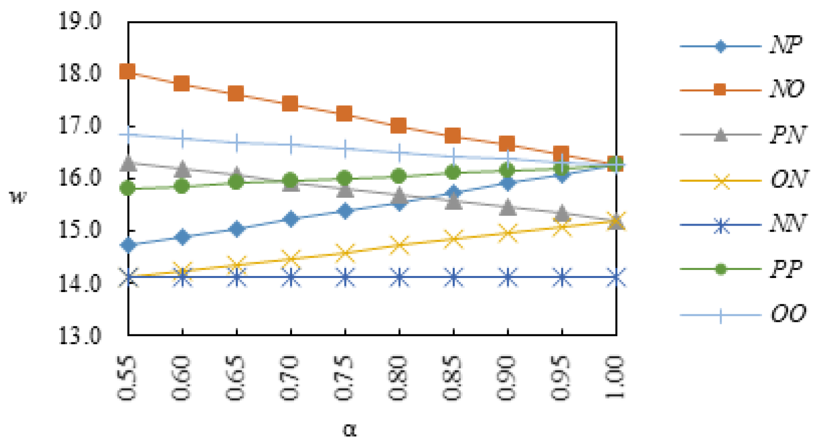
Observing Figure 4, it is obvious that the optimal outsourcing price is the highest in the NO model and the lowest in the NN model. With the confidence level $\alpha$ increasing, the values of $w^{*}$ generate an increase in the ON, PP, and NP models and a decrease in the PN, OO, and NO models. Moreover, there are $w_{NO}^{*}>w_{NP}^{*}$, $w_{OO}^{*}>w_{PP}^{*}$, and $w_{PN}^{*}>w_{ON}^{*}$ at all confidence levels.

The relationships among the optimal outsourcing prices under different risk preferences in Figure 4 are as follows:

$$\left\{\begin{array}{c}\hfill 0.55<\alpha \le 0.56,w_{NO}^{*}>w_{OO}^{*}>w_{PN}^{*}>w_{PP}^{*}>w_{NP}^{*}>w_{NN}^{*}>w_{ON}^{*}\\ \hfill 0.56<\alpha \le 0.70,w_{NO}^{*}>w_{OO}^{*}>w_{PN}^{*}>w_{PP}^{*}>w_{NP}^{*}>w_{ON}^{*}>w_{NN}^{*}\\ \hfill 0.70<\alpha \le 0.82,w_{NO}^{*}>w_{OO}^{*}>w_{PP}^{*}>w_{PN}^{*}>w_{NP}^{*}>w_{ON}^{*}>w_{NN}^{*}\\ \hfill 0.82<\alpha <1.00,w_{NO}^{*}>w_{OO}^{*}>w_{PP}^{*}>w_{NP}^{*}>w_{PN}^{*}>w_{ON}^{*}>w_{NN}^{*}\\ \hfill \alpha =1.00,w_{NP}^{*}=w_{NO}^{*}=w_{OO}^{*}=w_{PP}^{*}>w_{PN}^{*}=w_{ON}^{*}>w_{NN}^{*}\end{array}\right.$$

Figure 5 demonstrates that the optimal price is the highset in the OO model and the lowest in the NP model. Considering the increseaing change in the confidence level $\alpha$, the values of $p^{*}$ display an upward trend in the PN, PP, and NP models but a decline in the ON, OO, and NO models. Moreover, there are $p_{OO}^{*}>p_{PP}^{*}$, $p_{ON}^{*}>p_{PN}^{*}$ and $p_{NO}^{*}>p_{NP}^{*}$ at all confidence levels.

The relationships among the optimal price under different risk preferences in Figure 5 are as follows:

$$\left\{\begin{array}{c}\hfill 0.55<\alpha \le 0.58,p_{OO}^{*}>p_{ON}^{*}>p_{PP}^{*}>p_{NO}^{*}>p_{PN}^{*}>p_{NN}^{*}>p_{NP}^{*}\\ \hfill 0.58<\alpha \le 0.66,p_{OO}^{*}>p_{ON}^{*}>p_{PP}^{*}>p_{PN}^{*}>p_{NO}^{*}>p_{NN}^{*}>p_{NP}^{*}\\ \hfill 0.66<\alpha <0.83,p_{OO}^{*}>p_{ON}^{*}>p_{PP}^{*}>p_{PN}^{*}>p_{NN}^{*}>p_{NO}^{*}>p_{NP}^{*}\\ \hfill 0.83<\alpha <1.00,p_{OO}^{*}>p_{PP}^{*}>p_{ON}^{*}>p_{PN}^{*}>p_{NN}^{*}>p_{NO}^{*}>p_{NP}^{*}\\ \hfill \alpha =1.00,p_{OO}^{*}=p_{PP}^{*}>p_{PN}^{*}=p_{ON}^{*}>p_{NN}^{*}>p_{NO}^{*}=p_{NP}^{*}\end{array}\right.$$

As shown in Figure 6, the optimal marginal profit is the highset in the ON model and the lowest in NO model. With the increasing change in the confidence level $\alpha$, the values of $m^{*}$ show an upward trend in the PN, PP, and NO models but a decline in the NP, OO, and NO models. Moreover, there are $m_{ON}^{*}>m_{PN}^{*}$, $m_{OO}^{*}>m_{PP}^{*}$, and $m_{NP}^{*}>m_{NO}^{*}$ at all confidence levels.

The relationships among the optimal marginal profit of the LSI under different risk preferences in Figure 6 are as follows:

$$\left\{\begin{array}{c}\hfill 0.55<\alpha \le 0.64,m_{ON}^{*}>m_{OO}^{*}>m_{NN}^{*}>m_{PP}^{*}>m_{NP}^{*}>m_{PN}^{*}>m_{NO}^{*}\\ \hfill 0.64<\alpha <1.00,m_{ON}^{*}>m_{OO}^{*}>m_{NN}^{*}>m_{PP}^{*}>m_{PN}^{*}>m_{NP}^{*}>m_{NO}^{*}\\ \hfill \alpha =1.00,m_{PN}^{*}=m_{ON}^{*}=m_{NN}^{*}=m_{OO}^{*}=m_{PP}^{*}>m_{NO}^{*}=m_{NP}^{*}\end{array}\right.$$

5.2.2. Impact of $\alpha$ on ${\tilde{c}}_P^{*}$, ${\pi }_{SC}^{*}$, ${\pi }_P^{*}$, and ${\pi }_I^{*}$

In this section, we discuss the impacts of the risk preference on the optimal green innovation cost and profit through different confidence level $\alpha$ setting. Figure 7 shows that the optimal green innovation cost is the highset in the OO model and the lowest in the NP model. As the confidence level $\alpha$ increasingly changes, the values of ${\tilde{c}}_P^{*}$ display an upward trend in the ON, PP, and NP models but a decline in the PN, OO, and NO models. Furthermore, there are ${{\tilde{c}}_{\mathit{P}}^{*}}_{\mathit{OO}}>{{\tilde{c}}_{\mathit{P}}^{*}}_{\mathit{PP}}$, ${{\tilde{c}}_{\mathit{P}}^{*}}_{\mathit{PN}}>{{\tilde{c}}_{\mathit{P}}^{*}}_{\mathit{ON}}$, and ${{\tilde{c}}_{\mathit{P}}^{*}}_{\mathit{NO}}>{{\tilde{c}}_{\mathit{P}}^{*}}_{\mathit{NP}}$ at all confidence levels.

The relationships among the optimal green innovation cost under different risk preferences in Figure 7 are as follows:

$$\left\{\begin{array}{c}\hfill 0.55<\alpha \le 0.73,{{\tilde{c}}_{\mathit{P}}^{*}}_{\mathit{OO}}>{{\tilde{c}}_{\mathit{P}}^{*}}_{\mathit{PN}}>{{\tilde{c}}_{\mathit{P}}^{*}}_{\mathit{NN}}>{{\tilde{c}}_{\mathit{P}}^{*}}_{\mathit{ON}}>{{\tilde{c}}_{\mathit{P}}^{*}}_{\mathit{PP}}>{{\tilde{c}}_{\mathit{P}}^{*}}_{\mathit{NO}}>{{\tilde{c}}_{\mathit{P}}^{*}}_{\mathit{NP}}\\ \hfill 0.73<\alpha \le 0.83,{{\tilde{c}}_{\mathit{P}}^{*}}_{\mathit{OO}}>{{\tilde{c}}_{\mathit{P}}^{*}}_{\mathit{NN}}>{{\tilde{c}}_{\mathit{P}}^{*}}_{\mathit{PN}}>{{\tilde{c}}_{\mathit{P}}^{*}}_{\mathit{ON}}>{{\tilde{c}}_{\mathit{P}}^{*}}_{\mathit{PP}}>{{\tilde{c}}_{\mathit{P}}^{*}}_{\mathit{NO}}>{{\tilde{c}}_{\mathit{P}}^{*}}_{\mathit{NP}}\\ \hfill 0.83<\alpha \le 0.93,{{\tilde{c}}_{\mathit{P}}^{*}}_{\mathit{OO}}>{{\tilde{c}}_{\mathit{P}}^{*}}_{\mathit{NN}}>{{\tilde{c}}_{\mathit{P}}^{*}}_{\mathit{PN}}>{{\tilde{c}}_{\mathit{P}}^{*}}_{\mathit{PP}}>{{\tilde{c}}_{\mathit{P}}^{*}}_{\mathit{ON}}>{{\tilde{c}}_{\mathit{P}}^{*}}_{\mathit{NO}}>{{\tilde{c}}_{\mathit{P}}^{*}}_{\mathit{NP}}\\ \hfill 0.93<\alpha <1.00,{{\tilde{c}}_{\mathit{P}}^{*}}_{\mathit{OO}}>{{\tilde{c}}_{\mathit{P}}^{*}}_{\mathit{NN}}>{{\tilde{c}}_{\mathit{P}}^{*}}_{\mathit{PP}}>{{\tilde{c}}_{\mathit{P}}^{*}}_{\mathit{PN}}>{{\tilde{c}}_{\mathit{P}}^{*}}_{\mathit{ON}}>{\tilde{c}}_P{{}_{NO}}^{*}>{{\tilde{c}}_{\mathit{P}}^{*}}_{\mathit{NP}}\\ \hfill \alpha =1.00,{{\tilde{c}}_{\mathit{P}}^{*}}_{\mathit{NN}}>{{\tilde{c}}_{\mathit{P}}^{*}}_{\mathit{PP}}={{\tilde{c}}_{\mathit{P}}^{*}}_{\mathit{OO}}>{{\tilde{c}}_{\mathit{P}}^{*}}_{\mathit{PN}}={{\tilde{c}}_{\mathit{P}}^{*}}_{\mathit{ON}}>{\tilde{c}}_P{{}_{NO}}^{*}={{\tilde{c}}_{\mathit{P}}^{*}}_{\mathit{NP}}\end{array}\right.$$

As shown in Figure 8, it is obvious that when the confidence level $\alpha$ becomes close to 1, the optimal total profit of the LSSC in the NN model is the highest and is the lowest in the OO model. Moreover, as $\alpha$ increasingly changes, the optimal total profit of the LSSC show an upward trend in the NP, PN, PP, OO, and ON models. Howerver, it is only in the NO model that the optimal total profit of the LSSC declines. Moreover, there are ${{\pi }_{SC}}_{PP}^{*}>{{\pi }_{SC}}_{OO}^{*}$, ${{\pi }_{SC}}_{PN}^{*}>{{\pi }_{SC}}_{ON}^{*}$, and ${{\pi }_{SC}}_{NO}^{*}>{{\pi }_{SC}}_{NP}^{*}$ at all confidence levels.

The relationships among the optimal total profits of the LSSC under different risk preferences in Figure 8 are as follows:

$$\left\{\begin{array}{c}\hfill 0.55<\alpha \le 0.66,{{\pi }_{SC}}_{NO}^{*}>{{\pi }_{SC}}_{NN}^{*}>{{\pi }_{SC}}_{NP}^{*}>{{\pi }_{SC}}_{PN}^{*}>{{\pi }_{SC}}_{PP}^{*}>{{\pi }_{SC}}_{ON}^{*}>{{\pi }_{SC}}_{OO}^{*}\\ \hfill 0.66<\alpha \le 0.74,{{\pi }_{SC}}_{NO}^{*}>{{\pi }_{SC}}_{NN}^{*}>{{\pi }_{SC}}_{NP}^{*}>{{\pi }_{SC}}_{PN}^{*}>{{\pi }_{SC}}_{ON}^{*}>{{\pi }_{SC}}_{PP}^{*}>{{\pi }_{SC}}_{OO}^{*}\\ \hfill 0.74<\alpha <1.00,{{\pi }_{SC}}_{NN}^{*}>{{\pi }_{SC}}_{NO}^{*}>{{\pi }_{SC}}_{NP}^{*}>{{\pi }_{SC}}_{PN}^{*}>{{\pi }_{SC}}_{ON}^{*}>{{\pi }_{SC}}_{PP}^{*}>{{\pi }_{SC}}_{OO}^{*}\\ \hfill \alpha =1.00,{{\pi }_{SC}}_{NN}^{*}>{{\pi }_{SC}}_{NO}^{*}={{\pi }_{SC}}_{NP}^{*}>{{\pi }_{SC}}_{PN}^{*}={{\pi }_{SC}}_{ON}^{*}>{{\pi }_{SC}}_{OO}^{*}={{\pi }_{SC}}_{PP}^{*}\end{array}\right.$$

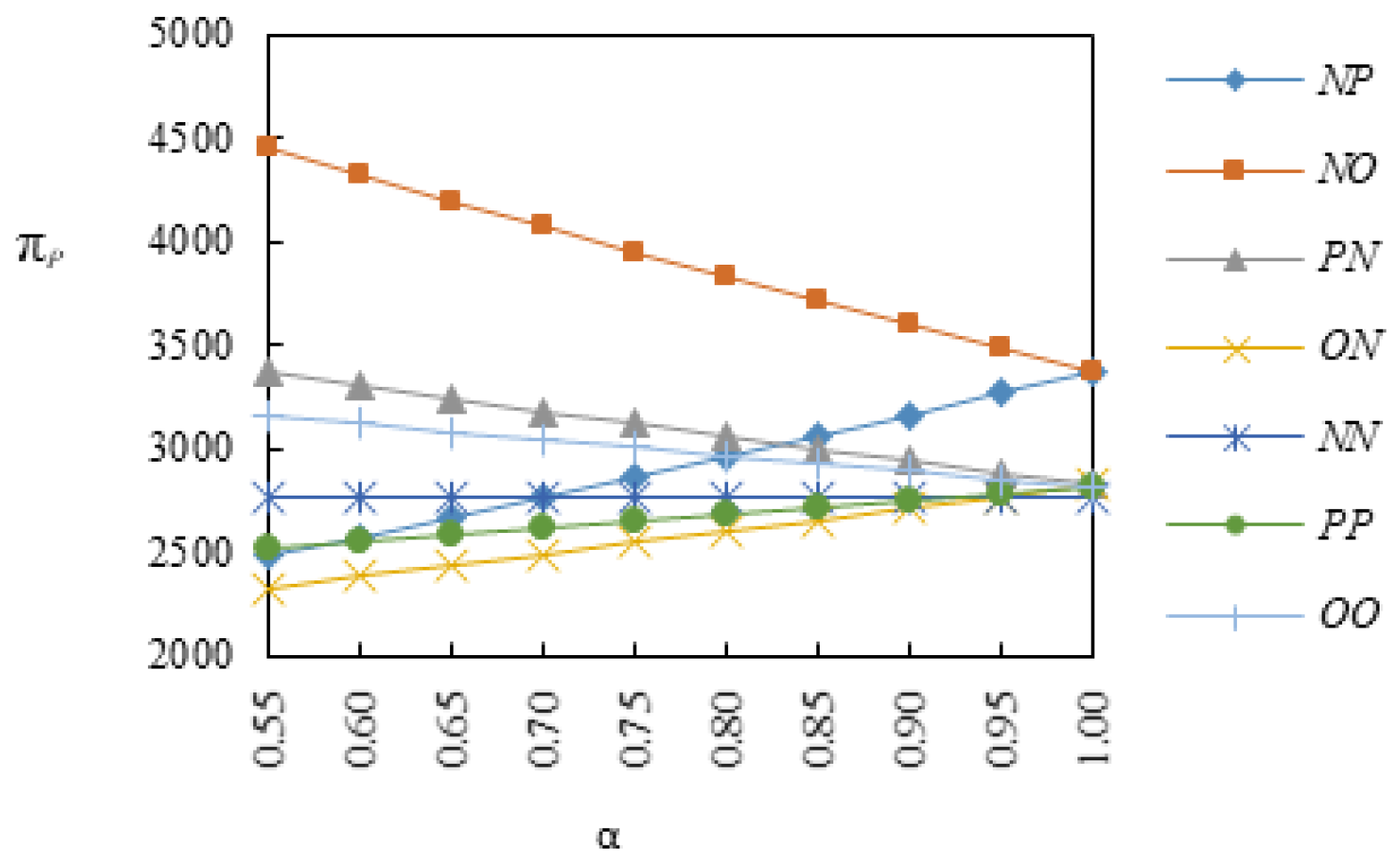
In Figure 9, we can see that the optimal profit for the LSP is the highset in the NO model, and it is initially the lowest in the ON model first and then in the NN model. Considering the increasing change in the confidence level $\alpha$, the values of ${\pi }_P^{*}$ display an upward trend in the NP, PP, and ON models but decline in model the PN, OO, and NO models. Still, there are ${{\pi }_P}_{OO}^{*}>{{\pi }_P}_{PP}^{*}$, ${{\pi }_P}_{PN}^{*}>{{\pi }_P}_{ON}^{*}$, and ${{\pi }_P}_{NO}^{*}>{{\pi }_P}_{NP}^{*}$ at all confidence levels.

It can be seen in Figure 9 that the relationships among the optimal profits of the LSP under different risk preferences are as follows:

$$\left\{\begin{array}{c}\hfill 0.55<\alpha \le 0.58,{{\pi }_P}_{NO}^{*}>{{\pi }_P}_{PN}^{*}>{{\pi }_P}_{OO}^{*}>{{\pi }_P}_{NN}^{*}>{{\pi }_P}_{PP}^{*}>{{\pi }_P}_{NP}^{*}>{{\pi }_P}_{ON}^{*}\\ \hfill 0.58<\alpha \le 0.70,{{\pi }_P}_{NO}^{*}>{{\pi }_P}_{PN}^{*}>{{\pi }_P}_{OO}^{*}>{{\pi }_P}_{NN}^{*}>{{\pi }_P}_{NP}^{*}>{{\pi }_P}_{PP}^{*}>{{\pi }_P}_{ON}^{*}\\ \hfill 0.70<\alpha <0.80,{{\pi }_P}_{NO}^{*}>{{\pi }_P}_{PN}^{*}>{{\pi }_P}_{OO}^{*}>{{\pi }_P}_{NP}^{*}>{{\pi }_P}_{NN}^{*}>{{\pi }_P}_{PP}^{*}>{{\pi }_P}_{ON}^{*}\\ \hfill 0.80<\alpha \le 0.84,{{\pi }_P}_{NO}^{*}>{{\pi }_P}_{PN}^{*}>{{\pi }_P}_{NP}^{*}>{{\pi }_P}_{OO}^{*}>{{\pi }_P}_{NN}^{*}>{{\pi }_P}_{PP}^{*}>{{\pi }_P}_{ON}^{*}\\ \hfill 0.84<\alpha \le 0.92,{{\pi }_P}_{NO}^{*}>{{\pi }_P}_{NP}^{*}>{{\pi }_P}_{PN}^{*}>{{\pi }_P}_{OO}^{*}>{{\pi }_P}_{NN}^{*}>{{\pi }_P}_{PP}^{*}>{{\pi }_P}_{ON}^{*}\\ \hfill 0.92<\alpha \le 0.94,{{\pi }_P}_{NO}^{*}>{{\pi }_P}_{NP}^{*}>{{\pi }_P}_{PN}^{*}>{{\pi }_P}_{OO}^{*}>{{\pi }_P}_{PP}^{*}>{{\pi }_P}_{NN}^{*}>{{\pi }_P}_{ON}^{*}\\ \hfill 0.94<\alpha <1.00,{{\pi }_P}_{NO}^{*}>{{\pi }_P}_{NP}^{*}>{{\pi }_P}_{PN}^{*}>{{\pi }_P}_{OO}^{*}>{{\pi }_P}_{PP}^{*}>{{\pi }_P}_{ON}^{*}>{{\pi }_P}_{NN}^{*}\\ \hfill \alpha =1.00,{{\pi }_P}_{NO}^{*}={{\pi }_P}_{NP}^{*}>{{\pi }_P}_{PN}^{*}={{\pi }_P}_{ON}^{*}>{{\pi }_P}_{PP}^{*}={{\pi }_P}_{OO}^{*}>{{\pi }_P}_{NN}^{*}\end{array}\right.$$

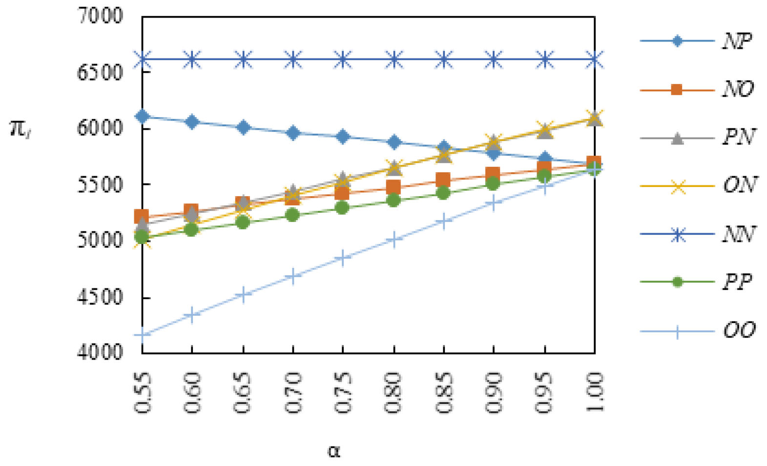
As shown in Figure 10, we can determine that the profit for the LSI is the highset in NN model and lowest in OO model. With the increasing changes in the confidence level $\alpha$, the values of ${\pi }_I^{*}$ display an upward trend in the PP, OO, ON, PN, and NO models but only decline in the NP model. In addition, there are ${{\pi }_I}_{PP}^{*}>{{\pi }_I}_{OO}^{*}$ and ${{\pi }_I}_{NP}^{*}>{{\pi }_I}_{NO}^{*}$ at all confidence levels.

Figure 10 demonstrates that the relationships among the optimal profit of the LSI under different risk preferences are as follows:

$$\left\{\begin{array}{c}\hfill 0.55<\alpha \le 0.57,{{\pi }_I}_{NN}^{*}>{{\pi }_I}_{NP}^{*}>{{\pi }_I}_{NO}^{*}>{{\pi }_I}_{PN}^{*}>{{\pi }_I}_{PP}^{*}>{{\pi }_I}_{ON}^{*}>{{\pi }_I}_{OO}^{*}\\ \hfill 0.57<\alpha \le 0.63,{{\pi }_I}_{NN}^{*}>{{\pi }_I}_{NP}^{*}>{{\pi }_I}_{NO}^{*}>{{\pi }_I}_{PN}^{*}>{{\pi }_I}_{ON}^{*}>{{\pi }_I}_{PP}^{*}>{{\pi }_I}_{OO}^{*}\\ \hfill 0.63<\alpha \le 0.68,{{\pi }_I}_{NN}^{*}>{{\pi }_I}_{NP}^{*}>{{\pi }_I}_{PN}^{*}>{{\pi }_I}_{NO}^{*}>{{\pi }_I}_{ON}^{*}>{{\pi }_I}_{PP}^{*}>{{\pi }_I}_{OO}^{*}\\ \hfill 0.68<\alpha \le 0.86,{{\pi }_I}_{NN}^{*}>{{\pi }_I}_{NP}^{*}>{{\pi }_I}_{PN}^{*}>{{\pi }_I}_{ON}^{*}>{{\pi }_I}_{NO}^{*}>{{\pi }_I}_{PP}^{*}>{{\pi }_I}_{OO}^{*}\\ \hfill {{0.86<\alpha <0.87,\pi }_I}_{NN}^{*}>{{\pi }_I}_{NP}^{*}>{{\pi }_I}_{ON}^{*}>{{\pi }_I}_{PN}^{*}>{{\pi }_I}_{NO}^{*}>{{\pi }_I}_{PP}^{*}>{{\pi }_I}_{OO}^{*}\\ \hfill 0.87\le \alpha <1.00,{{\pi }_I}_{NN}^{*}>{{\pi }_I}_{ON}^{*}>{{\pi }_I}_{PN}^{*}>{{\pi }_I}_{NP}^{*}>{{\pi }_I}_{NO}^{*}>{{\pi }_I}_{PP}^{*}>{{\pi }_I}_{OO}^{*}\\ \hfill \alpha =1.00,{{{{\pi }_I}_{NN}^{*}>{{\pi }_I}_{PN}^{*}={{\pi }_I}_{ON}^{*}>\pi }_I}_{NO}^{*}={{\pi }_I}_{NP}^{*}>{{\pi }_I}_{OO}^{*}={{\pi }_I}_{PP}^{*}\end{array}\right.$$

Figure 3, Figure 4, Figure 7 and Figure 9 display a definite trend in that the ${\theta }^{*}$, $w^{*}$, ${\tilde{c}}_P^{*}$, and ${\pi }_P^{*}$ demonstrate the same change with different confidence levels $\alpha$ in different scenarios. Specifically, they all decline in the NO, OO, and PN models and increase in the NP, ON, and PP models. Meanwhile, both ${\theta }^{*}$ and ${\tilde{c}}_P^{*}$ obtain the highest value in the OO model and lowest value in the NP model. Overall, all of the optimal solutions show a gradual upward trend in the PP model. When $\alpha$ becomes close to 1, both ${\pi }_{SC}^{*}$ and ${\pi }_I^{*}$ obtian the highest value in the NN model and lowest value in the OO model.

Extreme risk preference is ascribed to the value curves for ${\theta }^{*}$, $p^{*}$ and ${\tilde{c}}_P^{*}$ all being steeply downward sloping in the OO model and upward sloping in the PP model. With regard to the influence of variable determiners, the value curves for $w^{*}$ slope steeply upward in the NP model and decline in the NO model, while the curves for $m^{*}$ steeply decline in the ON model and increase in the PN model, and the curves for ${\pi }_P^{*}$ steeply decline in the NO model and increase in the NP model. Due to the extreme risk preference and the influence of the variable determiners, the value curves for ${\pi }_I^{*}$ all steeply rise in the OO and ON models. Taking into account the impact of the leading rights on the LSSC and participants’ risk preferences, the value curves for ${\pi }_{SC}^{*}$ all slope sharply upward in the ON, OO, and PP models, but steeply decline in the NO model.

6. Conclusions and Management Insights

6.1. The Main Conclusions

A win–win situation for the LSI and LSP can be achieved by forming an LSSC through which they can cooperate with one another. Additionally, logistics service operations play a significant role in reducing the environmental burden of the supply chain. Thus, green research on the LSSC is imperative. However, decision-makers have a vague understanding of the market environment of such green services due to the lack of reference historical data.

In order to explore the decision making problem in a two-stage LSSC with consideration of the influence of the environment, game theoretical models led by the LSI were developed in this paper to determine strategies for risk preference behavior selection and green service supply under a fuzzy environment. Subsequently, the optimal solutions of the LSP and the LSI were drawn. Then, numerical examples were presented to explore the impact of LSSC participants’ risk preference on the optimal solutions under the fuzzy environment. Based on the analysis and discussion above, we summarize and provide four conclusions as follows.

First, optimistic risk attitude can appropriately improve the greening level, price, and green innovation cost of logistics services. Of the various risk preference strategies, they all take maximum value when an optimistic LSP cooperates with a risk appetite LSI, and obtain minimum optimal solution in the NP model, in which a risk-neutral LSI works in cooperation with a risk-adverse LSP. In general, the greening level and green innovation cost in optimistic models are higher than those in pessimistic models.

Next, in terms of risk preference behavior, beyond a certain confidence level, both risk appetite and risk averse attitudes can also lead to a rise in the outsourcing price. When the confidence level is greater than 0.56, both the optimistic and pessimistic values of the outsourcing price are higher than the expected value. Specifically, it is clear that the risk preferences are ascribed to a higher outsourcing price.

Moreover, when the decision maker is risk neutral, the partner’s risk attitude has a significant effect on the value of the decision variables and cost. Taking into account that the greening level, outsourcing price, and green innovation cost are all determined by the LSP, the LSI determines the marginal profit. This is essential, because when one participant is risk-neutral, the partner’s risk preference plays a major role in the optimal solution. Moreover, the results were somewhat different from these of other models.

Finally, the optimal profits of the different risk preference behaviors between the LSI and LSP differ among various game models under fuzzy environments. Of the various risk preference strategies, to gain maximum profit, the best decision for the LSI is to remain neutral when the LSP is risk neutral; however, the LSP’s best decision is to adopt an optimistic attitude when the LSI is risk neutral, the LSP adopts an optimistic attitude. Furthermore, the total LSSC gains maximum profit in the NN model, which means that both the LSI and LSP remain risk-neutral, helping the supply chain to make a large profit.

6.2. Insights for Managers

A better understanding of the green logistics service supply chain game considering the impact of risk preference can offer better insight for logistics policymakers as to how to best make decisions under fuzzy environments. There are three important managerial implications of this study for LSSC games considering risk preference under fuzzy environments.

First, total involvement and cooperation among participants are vital factors for improving green management in the LSSC. The highest greening level is in the OO model, which means that only with a risk appetite LSI and LSP can the green and environmental level of the logistics service be significantly improved. This also shows that it is not only the LSP that can effectively affect the greening level; the LSI is also capable of this. Overall, to reduce the negative impact of logistics services on the environment, optimistic, full participation and effective cooperation of supply chain members are needed.

Secondly, risk preference plays a key role in how LSSC participants make decisions under fuzzy environments. The risk preference behavior of the LSI and LSP differs among the various game models under fuzzy environments. Of the various risk preference strategies, the best decision for the LSI is to be risk neutral when the LSP is risk neutral to obtain maximum profit. However, the LSP’s best decision for the greening level is to adopt an optimistic attitude to cooperate with the LSI.

Thirdly, the dominant position in a LSSC plays a crucial role in making profit. In our research, the LSI is the leader, and the profits of the LSI are always higher than those of the LSP in any risk preference model. Hence, the dominant leader in the LSSC, such as the LSI in this paper, obtains the higher profit, while the follower obtains the lower profit. Under these circumstances, it should be noted that in order to produce greater profit in the LSSC, participants must strive to improve their competitiveness to gain more control power.

7. Limitations and Future Work

This study focused on the decision making for the green LSSC composed of an LSI and an LSP with risk preference under fuzzy environments. Although our investigation provides useful management recommendations, there are still some limitations in this research. First, the theoretical model adopted in this study may be limited by certain technical assumptions used.

The assumptions of deterministic settings produced several limitations. For instance, we assumed that there was only one LSI and one LSP in the LSSC. This is a huge simplification of the real problem. Second, we only investigated the power structure led by LSI. There are other power structures in the real world. For instance, the LSSC may be dominated by the LSP or by both the LSP and LSI.

In the future, the proposed method can be applicable to other real-life problems, such as product pricing, supply chain contract design, and supplier selection. In addition, the demand function in this way was linear, and we can explore other forms of demand functions, such as stochastic demand functions. Finally, the inclusion of multiple competitive LSSC participants and other game power structures are also important directions for future research.

References

- Chen, W.; Hu, Z. Using evolutionary game theory to study governments and manufacturers’ behavioral strategies under various carbon taxes and subsidies. J. Clean. Prod. 2018, 201, 123–141. [Google Scholar] [CrossRef]
- Sun, L.; Cao, X.; Alharthi, M.; Zhang, J.; Taghizadeh-Hesary, F.; Mohsin, M. Carbon emission transfer strategies in supply chain with lag time of emission reduction technologies and low-carbon preference of consumers. J. Clean. Prod. 2020, 264, 121664. [Google Scholar] [CrossRef]
- Huang, S.; Fan, Z.; Wang, N. Green subsidy modes and pricing strategy in a capital-constrained supply chain. Transp. Res. Part E Logist. Transp. Rev. 2020, 136, 101885. [Google Scholar] [CrossRef]
- Jamali, M.; Rasti-Barzoki, M. A game theoretic approach to investigate the effects of third-party logistics in a sustainable supply chain by reducing delivery time and carbon emissions. J. Clean. Prod. 2019, 235, 636–652. [Google Scholar] [CrossRef]
- Widrick, R.S.; Nurre, S.G.; Robbins, M.J. Optimal policies for the management of an electric vehicle battery swap station. Transp. Sci. 2018, 52, 59–79. [Google Scholar] [CrossRef]
- Schneider, F.; Thonemann, U.W.; Klabjan, D. Optimization of battery charging and purchasing at electric vehicle battery swap stations. Transp. Sci. 2018, 52, 1211–1234. [Google Scholar] [CrossRef]
- Wang, S.; Hu, Z. Modeling green supply chain games considering retailer’s risk preference in fuzzy environment. Control Decis. 2021, 36, 711–723. [Google Scholar]
- Zhu, Q.; Sarkis, J.; Lai, K.-H. Institutional-based antecedents and performance outcomes of internal and external green supply chain management practices. J. Purch. Supply Manag. 2013, 19, 106–117. [Google Scholar] [CrossRef]
- Gao, Y.; Chang, D.; Fang, T.; Luo, T. The Correlation between Logistics Industry and Other Industries: An Evaluation of the Empirical Evidence from China. Asian J. Shipp. Logist. 2018, 34, 27–32. [Google Scholar] [CrossRef]
- Ju, Y.; Wang, Y.; Cheng, Y.; Jia, J. Investigating the Impact Factors of the Logistics Service Supply Chain for Sustainable Performance: Focused on Integrators. Sustainability 2019, 11, 538. [Google Scholar] [CrossRef] [Green Version]
- Colicchia, C.; Marchet, G.; Melacini, M.; Perotti, S. Building environmental sustainability: Empirical evidence from Logistics Service Providers. J. Clean. Prod. 2013, 59, 197–209. [Google Scholar] [CrossRef]
- Zailani, S.; Amran, A.; Jumadi, H. Green Innovation Adoption among Logistics Service Providers in Malaysia: An Exploratory Study on the Managers Perceptions. Int. Bus. Manag. 2011, 5, 104–113. [Google Scholar] [CrossRef] [Green Version]
- Li, D.F. Decision and Game Theory in Management with Intuitionistic Fuzzy Sets; Springer: Berlin/Heidelberg, Germany, 2014; pp. 14–26. [Google Scholar]
- Yu, G.; Li, D.; Fei, W. A novel method for heterogeneous multi-attribute group decision making with preference deviation. Comput. Ind. Eng. 2018, 124, 58–64. [Google Scholar] [CrossRef]
- McKinnon, A.; Browne, M.; Piecyk, M. Green Logistics: Improving the Environmental Sustainability of Logistics; Whiteing, A., Ed.; Kogan Page: London, UK, 2015; pp. 13–35. [Google Scholar]
- Lieb, K.J.; Lieb, R.C. Environmental sustainability in the third-party logistics (3PL) industry. Int. J. Phys. Distrib. Logist. Manag. 2010, 40, 524–533. [Google Scholar] [CrossRef]
- Zhu, Q.; Sarkis, J.; Lai, K.H. Confirmation of a measurement model for green supply chain management practices implementation. Int. J. Prod. Econ. 2008, 111, 261–273. [Google Scholar] [CrossRef]
- Dou, Y.; Zhu, Q.; Sarkis, J. Evaluating green supplier development programs with a grey-analytical network process-based methodology. Eur. J. Oper. Res. 2014, 233, 420–431. [Google Scholar] [CrossRef]
- Kellner, F.; Igl, J. Greenhouse gas reduction in transport: Analyzing the carbon dioxide performance of different freight forwarder networks. J. Clean. Prod. 2015, 99, 177–191. [Google Scholar] [CrossRef]
- Tan, C.; Li, B.; Cui, C. Analysis and Coordination of Logistics Service Supply Chain with Fairness Concerns considering Corporate Social Responsibility. Control Decis. 2020, 35, 1717–1729. [Google Scholar]
- De Oliveira, C.T.; Luna, M.M.M.; Campos, L.M.S. Understanding the Brazilian expanded polystyrene supply chain and its reverse logistics towards circular economy. J. Clean. Prod. 2019, 235, 562–573. [Google Scholar] [CrossRef]
- Maric, J.; Opazo-Basa’ez, M. Green Servitization for Flexible and Sustainable Supply Chain Operations A Review of Reverse Logistics Services in Manufacturing. Glob. J. Flex. Syst. Manag. 2019, 20, 65–80. [Google Scholar] [CrossRef]
- Liu, W.; Wang, Y. Quality control game model in logistics service supply chain based on different combinations of risk attitude. Int. J. Prod. Econ. 2015, 161, 181–191. [Google Scholar] [CrossRef]
- Liu, W.; Wang, D.; Shen, X.; Yan, X.; Wei, W. The impacts of distributional and peer-induced fairness concerns on the decision making of order allocation in logistics service supply chain. Transp. Res. Part E Logist. Transp. Rev. 2018, 116, 102–122. [Google Scholar] [CrossRef]
- Liu, W.; Wang, M.; Zhu, D.; Zhou, L. Service capacity procurement of logistics service supply chain with demand updating and loss-averse preference. Appl. Math. Model. 2019, 66, 486–507. [Google Scholar] [CrossRef]
- Du, N.; Zhou, S. Quality Defect Guarantee Decision in Logistics Service Supply Chain with Fairness Concern. Oper. Res. Manag. Sci. 2019, 28, 34–43. [Google Scholar]
- Demirel, S.; Kapuscinski, R.; Yu, M. Strategic Behavior of Suppliers in the Face of Production Disruptions. Manag. Sci. 2018, 64, 533–551. [Google Scholar] [CrossRef]
- Bimpikis, K.; Candogan, O.; Ehsani, S. Supply Disruptions and Optimal Network Structures. Manag. Sci. 2019, 65, 5504–5517. [Google Scholar] [CrossRef]
- Pan, S.; Zhong, R.Y.; Qu, T. Smart product-service systems in interoperable logistics: Design and implementation prospects. Adv. Eng. Inform. 2019, 42, 100996. [Google Scholar] [CrossRef]
- Zhang, C.; Fan, L.; Tian, Y. Optimal operational strategies of capital-constrained supply chain with logistics service and price dependent demand under 3PL financing service. Soft Comput. 2019, 24, 2793–2806. [Google Scholar] [CrossRef]
- Liu, X.; Zhang, K.; Chen, B.; Zhou, J.; Miao, L. Analysis of logistics service supply chain for the One Belt and One Road initiative of China. Transp. Res. Part E Logist. Transp. Rev. 2018, 117, 23–39. [Google Scholar] [CrossRef]
- Qin, X.; Su, Q.; Hong, Z. Competitive and cooperative strategies for online shopping logistics service supply chain considering customer expectations and quality cost. J. Ind. Eng./Eng. Manag. 2019, 33, 136–146. [Google Scholar]
- Giri, B.C.; Dey, S. Game theoretic models for a closed-loop supply chain with stochastic demand and backup supplier under dual channel recycling. Decis. Mak. Appl. Manag. Eng. 2020, 3, 108–125. [Google Scholar]
- Samanta, B.; Giri, B.C. A two-echelon supply chain model with price and warranty dependent demand and pro-rata warranty policy under cost sharing contract. Decis. Making Appl. Manag. Eng. 2021, 4, 47–75. [Google Scholar] [CrossRef]
- Liu, W.; Wang, Q.; Mao, Q.; Wang, S.; Zhu, D. A scheduling model of logistics service supply chain based on the mass customization service and uncertainty of FLSP’s operation time. Transp. Res. Part E Logist. Transp. Rev. 2015, 83, 189–215. [Google Scholar] [CrossRef]
- Liu, W.; Wu, R.; Liang, Z.; Zhu, D. Decision model for the customer order decoupling point considering order insertion scheduling with capacity and time constraints in logistics service supply chain. Appl. Math. Model. 2018, 54, 112–135. [Google Scholar] [CrossRef]
- Hu, X.; Wang, G.; Li, X.; Zhang, Y.; Feng, S.; Yang, A. Joint decision model of supplier selection and order allocation for the mass customization of logistics services. Transp. Res. Part E Logist. Transp. Rev. 2018, 120, 76–95. [Google Scholar] [CrossRef]
- Wang, G.; Hu, X.; Li, X.; Zhang, Y.; Feng, S.; Yang, A. Multiobjective decisions for provider selection and order allocation considering the position of the CODP in a logistics service supply chain. Comput. Ind. Eng. 2020, 140, 106216. [Google Scholar] [CrossRef]
- Wang, S. A Manufacturer Stackelberg Game in Price Competition Supply Chain under a Fuzzy Decision Environment. IAENG Int. J. Appl. Math. 2017, 47, 49–55. [Google Scholar]
- Liu, B.; Iwamura, K. Chance constrained programming with fuzzy parameters. Fuzzy Sets Syst. 1998, 94, 227–237. [Google Scholar] [CrossRef]
- Liu, B.; Liu, Y. Expected value of fuzzy variable and fuzzy expected value model. IEEE Trans. Fuzzy Syst. 2006, 10, 445–450. [Google Scholar]
- Lau, A.; Lau, H. Some two-echelon supply chian games: Improving form deterministics-symmetrics-information to stochstics asymmetrics-information models. Eur. J. Oper. Res. 2005, 161, 203–223. [Google Scholar] [CrossRef]
- Liu, B. Theory and Practice of Uncertain Programming; Physica: Heidelberg, Germany, 2002; pp. 25–29. [Google Scholar]
Figure 1.
The basic structure of a two-stage green LSSC.
Figure 2.
The LSI Stackelberg Game Decision Model.
Figure 3.
Greening level of the logistics with .
Figure 4.
Outsourcing price with .
Figure 5.
Price for the logistics service with .
Figure 6.
Margin profit of the LSI with .
Figure 7.
Green innovation cost with .
Figure 8.
Total profit of the LSSC with .
Figure 9.
The profit for the LSP with .
Figure 10.
The profit for the LSI with .