Article

Cost Minimizations and Performance Enhancements of Power Systems Using Spherical Prune Differential Evolution Algorithm Including Modal Analysis

by
Sherif S. M. Ghoneim
1,*,
Mohamed F. Kotb
2,
Hany M. Hasanien
3,
Mosleh M. Alharthi
1 and
Attia A. El-Fergany
4
1
Department of Electrical Engineering, College of Engineering, Taif University, Taif 21944, Saudi Arabia
2
Department of Electrical Engineering, Faculty of Engineering, Mansoura University, Mansoura 35516, Egypt
3
Electrical Power and Machines Department, Faculty of Engineering, Ain Shams University, Cairo 11517, Egypt
4
Electrical Power and Machines Department, Faculty of Engineering, Zagazig University, Zagazig 44519, Egypt
*
Author to whom correspondence should be addressed.
Sustainability 2021, 13(14), 8113; https://0-doi-org.brum.beds.ac.uk/10.3390/su13148113
Submission received: 29 June 2021 / Revised: 16 July 2021 / Accepted: 19 July 2021 / Published: 20 July 2021
(This article belongs to the Special Issue Advanced Renewable Energy for Sustainability)

Abstract

:
A novel application of the spherical prune differential evolution algorithm (SpDEA) to solve optimal power flow (OPF) problems in electric power systems is presented. The SpDEA has several merits, such as its high convergence speed, low number of parameters to be designed, and low computational procedures. Four objectives, complete with their relevant operating constraints, are adopted to be optimized simultaneously. Various case studies of multiple objective scenarios are demonstrated under MATLAB environment. Static voltage stability index of lowest/weak bus using modal analysis is incorporated. The results generated by the SpDEA are investigated and compared to standard multi-objective differential evolution (MODE) to prove their viability. The best answer is chosen carefully among trade-off Pareto points by using the technique of fuzzy Pareto solution. Two power system networks such as IEEE 30-bus and 118-bus systems as large-scale optimization problems with 129 design control variables are utilized to point out the effectiveness of the SpDEA. The realized results among many independent runs indicate the robustness of the SpDEA-based approach on OPF methodology in optimizing the defined objectives simultaneously.

1. Introduction

Till this moment, power networks remain one of the most complicated systems in industry due to many reasons, such as variation of generation and load demand, the inclusion of renewable energy systems, and storage devices. These power systems are entirely nonlinear systems, where many components including synchronous generators, transformers, transmission lines, and induction motors have a deep nonlinearity. The optimal operation of such components to achieve a concise economic target, emission minimization possibility, power loss reduction and other objectives under the power system constraints plays an important role in the power system operation and is named optimal power flow (OPF) [1,2,3,4,5]. This problem, as mentioned earlier, is consequently considered a significant nonlinear optimization problem. In this issue, some fitness functions can be sequentially solved under the system operating conditions, including fuel consumption cost (FC), pollution release rate, active power loss, reactive power loss, bus voltage declines and many more.
Previously, several classical mathematical optimization approaches have been employed to solve the OPF problem [6,7,8,9,10]. Among the said traditional methods are: (i) moment-based relaxations [6], (ii) linear and quadratic programming [7], (iii) decomposition of the network graph into a spanning tree and closed cycles [8], (iv) safety barrier interior- point approach [9], and (v) a semi-definite method [10]. Nevertheless, these traditional approaches have many disadvantages, including their dependency on the values of the problem initial conditions, solver type, and accuracy. It shall be stuck into a local solution under the OPF problem’s nonlinearity. For that reason, different heuristics-based optimization techniques have been developed for solving such problems. Principally, similar heuristic techniques are randomly initialed populations of their agents, and the suboptimal/optimal answer is based on their methodologies. Several optimization methods have been used to tackle the OPF problem whether the target is single or multiple objective functions, such as genetic procedures [11], particle swarm optimizer [12], imperialist competitive algorithm [13], chaotic invasive weed optimization algorithms [14], JAYA algorithm [15], shuffled-frog-leaping algorithm [16], social spider optimization algorithm [17], chaotic salp swarm optimizer [18], new adaptive partitioning flower pollination algorithm [19], and others [20,21,22,23,24,25,26,27,28,29,30,31,32,33,34,35,36,37,38].
Among these kinds of literature, as mentioned earlier, the reader can notice that an avalanche of articles is presented to solve OPF problems using differential evolution (DE) with various versions [23,34,35,36,37,38], in which the authors concluded the powerful features and advantages of DE in solving OPF problems. Few of these works are employed to solve simultaneous multiple conflicting objectives such as OPF problems. Principally, these reported studies indicate the great development of metaheuristic algorithms. Therefore, a novel spherical prune DE algorithm (SpDEA) is implemented to solve the multiple objective OPF problems in this study.
It is well-known that DE is considered a much-enhanced version of the genetic algorithm originally established by Storn and Price [39]. DE procedures have many variants for mutation schemes, such as DE/X/Y/Z, DE/best/2, DE/best/2, DE/rand/1/bin, and so on; each variant has its own advantage, and its performance relies on the nature of the problem to be optimized [40,41]. DE has many key advantageous items e.g., (i) it’s simple to apply with a very effective mutation process, (ii) DE has a comparatively smooth convergence at high speeds of processing, (iii) a smaller size of the population generally suffices for solving large-scale engineering problems, and (iv) accordingly, it can be confirmed that there are significant reductions in computation burdens placed on the computer processors. The SpDEA has the flexibility to select the best compromise Paretos within the search space, and this leads to obtaining the optimal point in a quick manner, representing good merit.
The problem defines the optimal settings of design variables of the network through optimizing various identified objectives under system operating and capacity constraints. The control variables involve the active power output, the generating units’ voltage, tap-changer adjustments, and reactive compensating apparatuses. The control variables are continuous except for the transformer tap settings, which are discrete, and its step is chosen ±1.25%. Many objective functions may be involved through the OPF formulation, such as FC of generating units, pollution rate released by these units, network real power loss, voltage deviation, etc.
In this article, a novel SpDEA is presented to solve different multiple objective OPF problems. The vector objective functions include the FC, network overall real power losses, voltage deviation index, and stability of power networks. Voltage stability analysis has attracted much interest. It relies on a modal analysis, which is represented as a fitness function. In this issue, the Jacobian matrix is reduced, and then eigenvalues and eigenvectors are determined. The amplitude of eigenvalues measures the system instability. When this amplitude increases, the incremental voltage decreases, indicating the system’s strong voltage stability. The output (active power) of the units, their voltages, tap settings of power transformers, and compensating devices represent the design control variables of the problem. The SpDEA is employed to solve the OPF problem for two medium-size systems: a 30-bus network and a large-scale system, for instance, 118-bus network under multiple objective functions. The value of the SpDEA is compared to that obtained by using other optimization techniques. The numerical results are performed on MATLAB software. The results achieved demonstrate a competition of the SpDEA with other competing methods to solve multi-objective OPF problems.
The paper is sectionalized and arranged as follows: Section 2 introduces OPF problem representations with the proposed objectives and their associated constraints. In Section 3, the SpDEA mathematical model and its general procedures are presented. Section 4 gives the simulation scenarios, numerical results, and discussions. In Section 5, final concluding remarks along with future trends are drawn.

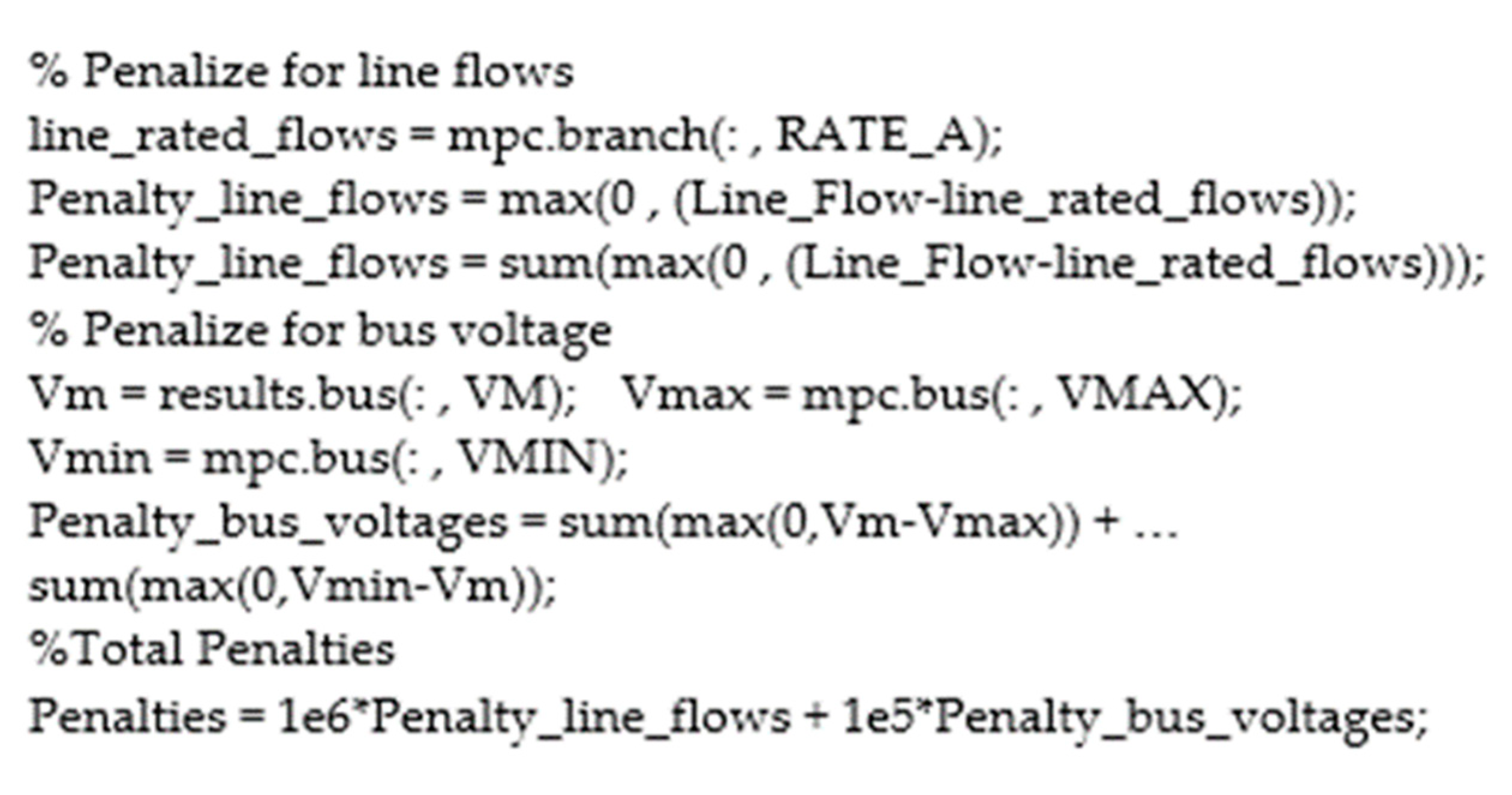
2. OPF Mathematical Representations

In this study, the optimization problem is expressed with four objectives for simultaneous optimization. The adopted objectives are depicted in (1)–(4):
T F C = i = 1 N g a i P G i 2 + b i P G i + c i
T P L = T G P T P D
T V D P Q = i = 1 N P Q | | V i | | V r e f | |
λ i = Δ Q m i   Δ V m i  
where T F C is the total FC of the generating units, P G i is the active output generating power at ith bus, a i , b i , c i are FC coefficients of ith generating unit, N g defines the number of generators, T P L is the system total active power loss, T G P is the total generated power, T P D is total power demand,   T V D P Q is the total voltage deviation of all PQ buses, | V r e f | is the reference voltage magnitude (typically, | V r e f | has a value of 1 per unit (pu)), N P Q defines the number of PQ buses,   λ i specifies the magnitude of eigen value, and Δ Q m i and   Δ V m i define the ith modal reactive power and voltage changes, respectively.
It is worth mentioning that the stability of the mode i is based on λ i . The largest λ i indicates slight variations of the modal voltage due to reactive power change. Therefore, the least value of λ i is chosen as a fourth objective, which requires upgrading for a better power system voltage stability. A further derivation regarding eigenvalues and eigenvectors for the modal analysis can be found in [42].
The aforementioned optimization problem undergoes to set of equality/inequality limitations such as:
P G i P D i = | V i | j = 1 N | V j | ( G i j c o s δ i j + B i j s i n δ i j ) Q G i Q D i = | V i | j = 1 N | V j | ( G i j s i n δ i j B i j c o s δ i j ) } ,   i   N
P G i m i n P G i P G i m a x Q G i m i n Q G i Q G i m a x } ,   i   N g
| V i m i n | | V i | | V i m a x | ,   i   N
t k m i n t k t k m a x ,   k   N t
S l i S l i r a t e d ,   i   n b r
Q c i m i n Q c i Q c i m a x ,   i   N c
where PDi is the active demand power at bus i; G i j and   B i j are the conductance and susceptance between bus i and j, respectively;   δ i j is the power angle between bus i and j; Q G i is the reactive power generation at bus i; Q D i is the load reactive demand power at bus i; P G i m i n , P G i m a x are the lower and higher limits of PGi, respectively; Q G i m i n , Q G i m a x are the min/max limits of Q G i , respectively; | V i m i n | , | V i m a x | are the min/max limits of | V i | , respectively; t k m i n , t k m a x are the min/max limits of tap settings of the kth transformer, respectively; N t defines the number of power transformers; S l i is apparent power flow in ith line; S l i r a t e d specifies the rated line maximum transfer capacity; n b r defines the number of network branches; Q c i m i n , Q c i m a x are the min/max limits of Q c i , respectively; and N c defines the number of nominated buses for capacitive devices.
In this study, the vector-defined objectives are solved using the SpDEA and are based on the fuzzification of Pareto fuzzy optimal (PFO) solutions. In this issue, the objective function O F i is expressed by a fuzzy membership function μ i to normalize the values between 0 and 1 as expressed in (11) [23]:
μ i = O F i O F i m i n O F i m a x O F i m i n
In addition, for each k-th Pareto solution, the normalized membership μ k is estimated by the formula depicted in (12):
μ k = i = 1 N o j μ i k k = 1 M i = 1 N o j μ i k , k M
where N o j and M define the number of objectives and the number of PFO solutions, respectively. The best compromise solution is chosen for the minimum value of μ k .

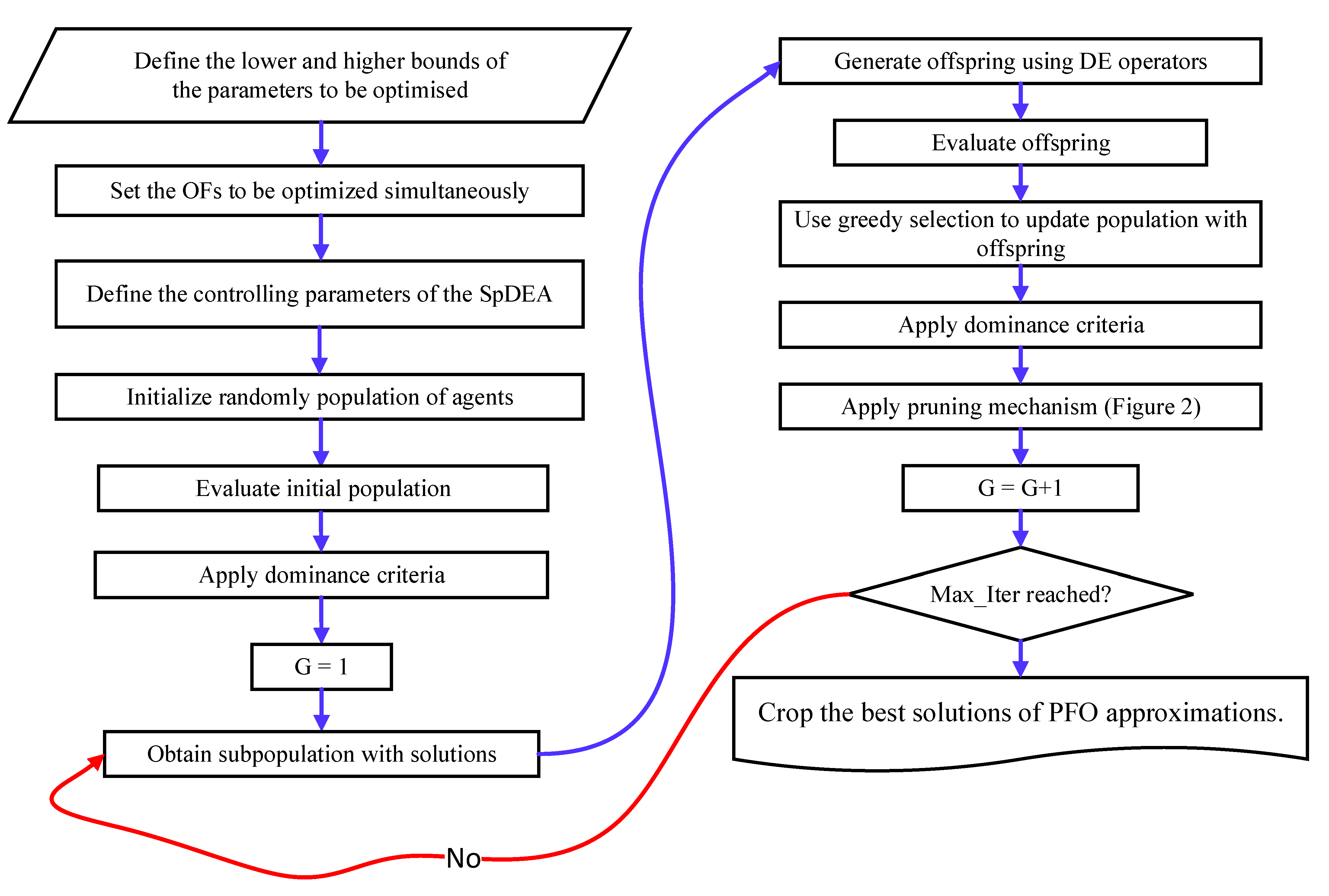
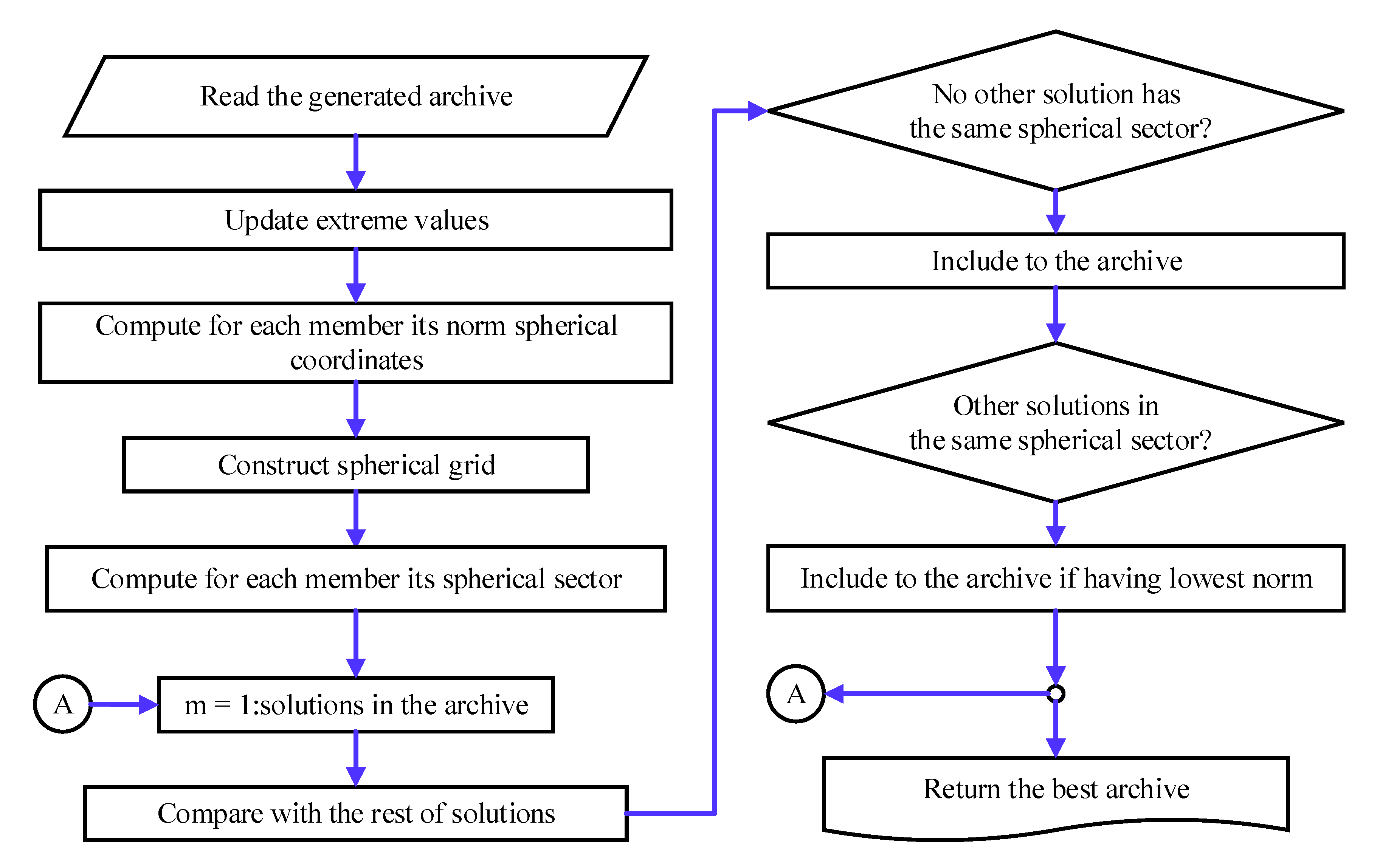
3. Mathematical Model of SpDEA

The main three strategies for the DE procedure include mutation, crossover, and selection stage. Similar to other challenging optimization methods, at initial stage, a vector of random positions ( x j , i ( 0 ) ) for the population is created within the predefined boundaries, which can be expressed in (13):
x j , i ( 0 ) = x j ,   m i n + r ( ) . ( x j ,   m a x x j ,   m i n ) ,   i P S ,     j d i m
where d i m defines the number of decision variables, P S is the population-size, r ( ) is a uniform random distribution function [ 0 ,   1 ] , and x j ,   m i n and x j ,   m a x are min/max limits of the jth decision control variable, respectively.
At this moment, the DE starts to mutate and to recombine the population to generate trial vectors x i . Then, DE implements a uniform crossover procedure to produce trial vectors x i . This is made by mixing x i and the target vector x i based on the crossover probability C R   ϵ   [ 0 , 1 ] , which is combined in a single formula as depicted in (14):
x j , i ( g ) = { x a ( g ) + . ( x b ( g ) x c ( g ) ) ,     i P S     i f   r j ( ) C R x j , i ( g )                   e l s e
where g is the iteration counter, x a is a base-vector and x b and x c are the difference trial vectors that are picked up randomly, factors of a , b , c , and i are unequal and defines the scaling factor ϵ [0, 1].
Then, a move is made to the new position, and as a final point, the collection occurs where a tournament is seized between the target and trial vectors, and the one with the best fitness value is endorsed to pass to the next generation. Through this, agents of a new generation are better than that of the previous ones.
The controlling parameters of the DE required for appropriate adaption by the users include and C R , along with those used with all other competing methods, such as the maximum iterations and PS . In common practice, the tuning of the DE-controlling factors is carried out by trial and error procedures to achieve a satisfactory performance of the DE algorithm.
This work cares by solving multiple objective optimization problems, such as the defined four objectives of OPF as stated in (1)–(4). SpDEA is applied to deal with such anticipated simultaneous objectives. Spherical pruning has been proposed by Reynoso-Meza [43,44] to improve diversity in the approximated PFO. Spherical coordinates are employed to partition the search space, and a selection of one solution is chosen in each spherical sector, evading congestion regions. SpDEA comprises actions to expand relevance applicability and to look effectively for a PFO approximation within the pertinency boundaries [45,46].
The principle motivation of the Sp is to investigate the offered solutions in the current PFO approximation using normalized spherical coordinates from a reference solution in the spherical sector. The general procedures of SpDEA are depicted in the flowchart shown in Figure 1. On the other hand, the detailed procedures of Sp mechanism are shown in Figure 2.
Further detailed explanation concerning the Sp definitions such as normalized spherical coordinates, sight range, spherical grid and sector, and so on, along with mathematical representations, can be obtained from [43,46]. The overall controlling parameters of SpDEA are , CR , PS , and the number of arcs that should be tuned sufficiently for better performance. Fuzzy-based decision-making methodology [23] is used to choose the best compromise among trade-off PFO points for various scenarios.

4. Numerical Simulations, Scenarios, and Discussions

This current study focuses on solving the OPF problem in power systems from the multi-objective function perspective using the proposed SpDEA. The problem codes are built with MATLAB software [47]. The OPF problem is solved by different IEEE standard systems such as 30 and 118-bus systems. The main features of these two systems are depicted in Table 1, extracted from [1,15,23].
The aforementioned four objective functions are combined to form different multi-objective functions through the OPF problem. The summary of various vector objectives of the OPF problem is demonstrated in Table 2. The computer simulations are performed using a PC (Intel(R) Core(TM) i7 2.4 GHz µP, 16 GB RAM, and Windows 10 system). The controlling parameters that adjust the performance of the SpDEA are specified in Table 3.
It is well-meaning to state that the power/load flow of the two systems under study is carried out using the full Newton–Raphson method implemented under MATPOWER [48]. It may be useful to state here some penalties added to the objective function (s) to produce a feasible solution. Among these penalties, the magnitude of bus voltages, power line flow, and reactive power of generating units are proposed. The typical MATLAB code to fulfill the condition of bus voltage and line flow limits is shown in Figure 3. The limitations of generating units’ reactive power are controlled through N-R LF, as illustrated in the next subsections. The studied cases of the OPF problem for these IEEE standard power systems are demonstrated in the following subsections comprising necessary validations, comparisons, and discussions. It might be worth mentioning that all runs are performed on a Laptop with Intel® Core™ i7-7700HQ CPU with 16 GB installed memory.

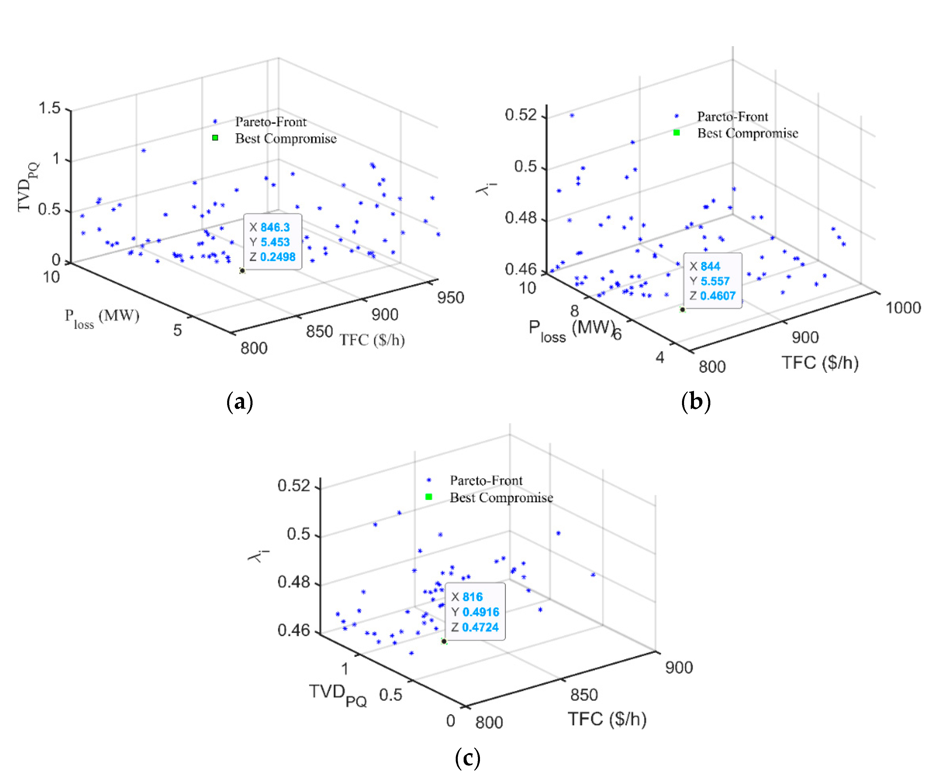
4.1. IEEE 30-Bus System

In this system, nine buses are nominated for capacitive shunt compensators at bus numbers of {10, 12, 15, 17, 20, 21, 23, 24, and 29} [15,23]. The network data are demonstrated in detail in [1,48]. The voltage magnitude of buses changes in the range 90–110%, the transformer taps settings lie in the range 90%–110% with a step of ±1.25%, and the reactive power of the shunt compensator is 5 MVAr. The SpDEA solves the different multiple objectives that are formulated in Table 2. The optimal characteristics of the SpDEA are revealed in Table 3. Many independent runs have been carried out to determine the optimal values of control variables. The optimal values of control variables and their corresponding fitness values are pointed out in Table 4.
It may be noted that in the N-R LF using MATPOWER, the option of “pf.enforce_q_lims“ is set to 1. As a result of activating this option, any generator’s reactive power exceeds the min/max limits after running the N-R LF, and the corresponding bus is converted to a PQ-bus, with Q g . If the reference bus is converted to PQ-bus, the first remaining PV-bus will be used as the slack bus for the next iteration at the limit, and the case is re-run. The voltage magnitude at the bus will deviate from the specified value to satisfy the reactive power limit. In other words, the relevant operating constraints of the reactive power output from the generators are maintained within practical operating points. The corresponding generator’s reactive power outputs are arranged in Table 5 of design settings for various objectives using the SpDEA.
Figure 4a–c illustrate PFO solutions and best compromise value for cases 1–3, representing the anticipated bi-objective cases. On the other hand, Figure 5a–c illustrate PFO solutions and best compromise value for cases 4–6, representing the anticipated tri-objective cases. It is worthy of note here that these Pareto optimal solutions lie in an acceptable range of minimization of each simultaneous objective function. Moreover, the best compromise value is located at a proper value within the suggested PFO solutions.
For a rational comparison, the SpDEA-based OPF results are compared with MODE and others, summarized in Table 6. It can be noted from this comparison that the best compromise values of OPF solutions using the SpDEA are very competitive, even though the TFC and TNL functions are contradictory. It reflects the proper design of the SpDEA to solve the multi-objective OPF problem in power systems. In addition to that, the average elapsed CPU times for various objectives’ scenarios are mentioned in the last row of Table 4. It may be noted that bold font indicates the best results obtained so far.

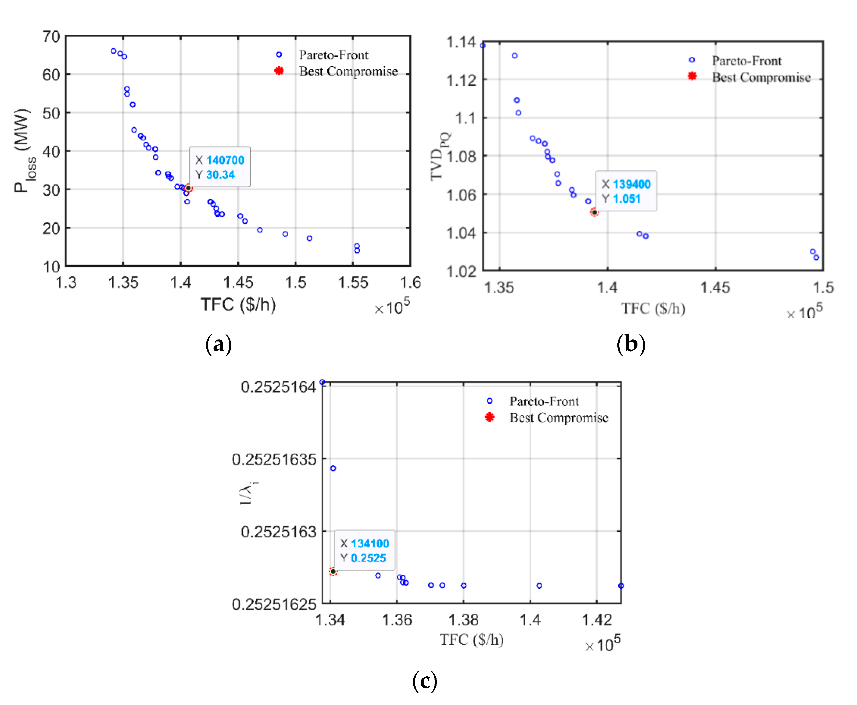
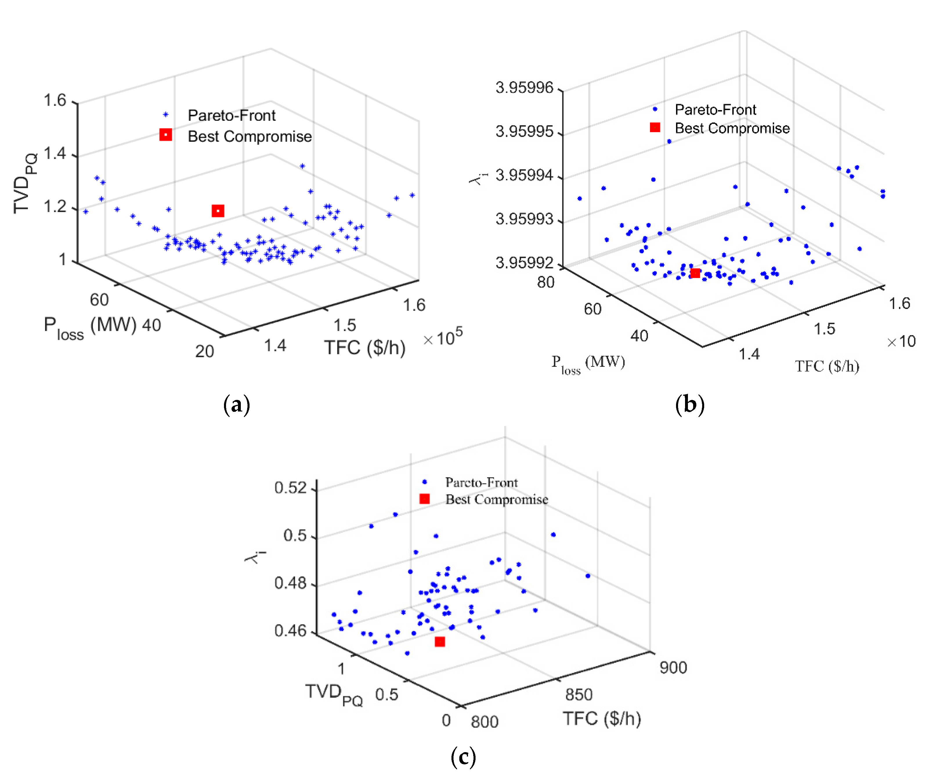
4.2. IEEE 118-Bus System

In this scenario, the SpDEA is applied to solve different vector objectives of the OPF problem for the standard 118-bus IEEE system [48] with the main features stated in Table 1. The capacitive compensating devices are installed on the bus numbers of {34, 44, 45, 46, 48, 74, 79, 82, 83, 105, 107, and 110} and its maximum rated capacity is 30 MVAr [19,22,23]. The data are demonstrated in detail in Table 2. The generating voltage magnitude of buses changes in the range 90–110%, the tap settings lie in the range 90%-110%. This optimization problem involves 129 control variables, posing a large challenge to the proposed algorithm. The optimal characteristics of the proposed SpDEA for this test case are demonstrated in Table 7 (last column). The various multiple objectives that are formulated in Table 2 are solved using the proposed SpDEA. The best values of control variables and their best compromise settings are recorded. However, the data of all cases are huge, and it is incredibly difficult to write in a paper. Therefore, only one case (case 1) is proposed, as illustrated in Table 7. The best compromise Pareto records 140,700 $/h and 30.339 MW to the TFC and TNL of the network. Figure 6a illustrates PFO solutions and best compromise value for case 1. It can be noted here that the SPDEA selects the best compromise Pareto within the search space. It is worthy to note here that these PFO solutions lie in an acceptable range of minimization of each simultaneous objective function.
Moreover, Figure 6b,c point out the PFO solutions and their corresponding best compromise for the other cases that include bi-objective functions (cases 2–3). On the other hand, Figure 7a–c indicate the PFO solutions and their corresponding best compromise for three simultaneous objective functions (cases 4–6). The best compromise values for all these cases lie in acceptable ranges that can be confirmed. In addition, the SpDEA is applied to case 7 for solving the multi-objective function that contains all four objectives. In this issue, the best compromise Pareto records 150,718 $/h, 33.69 MW, 1.415 pu, and 0.2525 to the TFC, TNL of the system, TVD for PQ buses, and voltage stability index, respectively. Therefore, it is successfully applied to various multiple adopted scenarios of the OPF problem regarding spot-on large-scale power systems.
Indeed, a fair comparison should be made between the proposed SpDEA-based OPF results and the MODE-based results to point out the flexibility, availability, and strength of the SpDEA-based OPF methodology. In this regard, Table 8 points out this detailed comparison for all seven cases. It is well-meaning here to say that the numerical results of the OPF problem using the SpDEA-based on OPF methodology are very similar to those obtained by the conventional MODE. The main merit of the proposed SpDEA is that it selects the best compromise among PFO solutions from several hundred Paretos within the search space. Moreover, the best compromise Paretos are within acceptable ranges. This property gives it a high possibility of reaching the optimal point in a quick way. This desired property is obviously illustrated in Figure 5. This reflects the proper design of the SpDEA to solve the multiple vector simultaneous objectives of the OPF problem in electric power networks.
At last, it can be concluded that the SpDEA proves its viability in solving a large-scale conventional power system such as a standard IEEE 118-bus network. It is well-known strategically that many countries worldwide have planned to increase their shares of renewable energy generation from sources such as solar, wind, tidal, and many more, including energy storage facilities [51,52,53]. As a result, such penetrations to conventional power systems increase uncertainty. Therefore, it is important to extend the existing frameworks/methodologies to address this challenge. The later mentioned defines the future trend of our current work by incorporating system uncertainties and the variability of different types of renewable power sources and loads.

5. Conclusions

A novel application of the spherical prune differential evolution algorithm has been demonstrated to solve the OPF problem in electric power schemes to achieve simultaneous objectives under various scenarios. The OPF problem has been investigated with the well-known IEEE standard 30-bus and 118-bus networks as a large-scale optimization problem with 129 design control variables. All constraints have been respected with no violations. MATPOWER has been used to implement the full load flow analysis of the networks under study using full Newton–Raphson method. PFO solutions are generated, and the best settings are carefully selected by using the technique of normalized fuzzifications. The best results for the IEEE 30-bus system with quad objectives of TFC, TPL, TVD PQ and 1/λi are equal to 840.92 $/h, 5.89 MW, 9458 PU and 1.879, respectively. On the other hand, for the best results for the IEEE 118-bus system are equal to 150,718 ($/h), 33.6933 MW, 1.41465 PU and 0.252516 for the same quad objectives, respectively. The demonstrated numerical simulations using the proposed SpDEA-based OPF methodology have proved their high performance, effectiveness, and robustness for solving the OPF problem of power systems in comparison to others reported in the literature.
Since the shares of renewable power sources including energy storage facilities are booming, uncertainty is increasing. Therefore, it is important to extend the existing frameworks/methodologies to address this challenge. The later mentioned defines the future trend of our current work by incorporating system uncertainties and the variability of different types of renewable power sources and loads.

Author Contributions

Conceptualization, S.S.M.G., M.F.K. and A.A.E.-F.; methodology, S.S.M.G., M.F.K., H.M.H. and A.A.E.-F.; software, M.F.K., A.A.E.-F. and S.S.M.G.; validation, A.A.E.-F., M.F.K. and S.S.M.G.; formal analysis, H.M.H., M.F.K. and S.S.M.G.; investigation, M.F.K., A.A.E.-F. and H.M.H.; resources, S.S.M.G., M.F.K. and M.M.A.; data curation, S.S.M.G., M.F.K. and A.A.E.-F.; writing—original draft preparation, S.S.M.G., M.F.K. and A.A.E.-F.; writing—review and editing, M.F.K., A.A.E.-F. and H.M.H.; visualization S.S.M.G., A.A.E.-F. and M.F.K.; supervision, A.A.E.-F., S.S.M.G. and M.M.A.; project administration, A.A.E.-F., M.M.A. and S.S.M.G.; funding acquisition, M.M.A. All authors have read and agreed to the published version of the manuscript.

Funding

This project is funded by Taif University Researchers Supporting Project under Grant TURSP-2020/122, Taif, Saudi Arabia.

Institutional Review Board Statement

The study did not involve humans or animals.

Informed Consent Statement

The study did not involve humans.

Data Availability Statement

Not applicable.

Acknowledgments

This work was supported by the Taif University, Taif, Saudi Arabia, through the Taif University Researchers Supporting Project under Grant TURSP-2020/122.

Conflicts of Interest

The authors declare no conflict of interest.

References

  1. Wood, A.J.; Wollenberg, B.F.; Sheblé, G.B. Power Generation, Operation, and Control, 3rd ed.; Wiley: New York, NY, USA, 2013; ISBN 978-0-471-79055-6. [Google Scholar]
  2. Bu, C.; Luo, W.; Zhu, T.; Yi, R.; Yang, B. Species and memory enhanced differential evolution for optimal power flow under double-sided uncertainties. IEEE Trans. Sustain. Comput. 2020, 5, 403–415. [Google Scholar] [CrossRef]
  3. Zhu, T.; Luo, W.; Bu, C.; Yue, L. Accelerate population-based stochastic search algorithms with memory for optima tracking on dynamic power systems. IEEE Trans. Power Syst. 2016, 31, 268–277. [Google Scholar] [CrossRef]
  4. Biswas, P.; Suganthan, P.; Amaratunga, G. Optimal power flow solutions using algorithm success history based adaptive differential evolution with linear population reduction. In Proceedings of the IEEE International Conference on Systems, Man, and Cybernetics, Miyazaki, Japan, 7–10 October 2018. [Google Scholar] [CrossRef]
  5. Biswas, P.; Suganthan, P.; Qu, B.Y.; Amaratunga, G. Multiobjective economic-environmental power dispatch with stochastic wind-solar-small hydro power. Energy 2018, 150, 1039–1057. [Google Scholar] [CrossRef]
  6. Molzahn, D.K.; Hiskens, I.A. Sparsity-exploiting moment-based relaxations of the optimal power flow problem. IEEE Trans. Power Syst. 2015, 30, 3168–3180. [Google Scholar] [CrossRef]
  7. Fortenbacher, P.; Demiray, T. Linear/quadratic programming-based optimal power flow using linear power flow and absolute loss approximations. Int. J. Electr. Power Energy Syst. 2019, 107, 680–689. [Google Scholar] [CrossRef] [Green Version]
  8. Hörsch, J.; Ronellenfitsch, H.; Witthaut, D.; Brown, T. Linear optimal power flow using cycle flows. Electr. Power Syst. Res. 2018, 158, 126–135. [Google Scholar] [CrossRef] [Green Version]
  9. Oliveira, E.J.; Oliveira, L.W.; Pereira, J.L.R.; Honório, L.M.; Marcato, A.L.M. An optimal power flow based on safety barrier interior point method. Int. J. Electr. Power Energy Syst. 2015, 64, 977–985. [Google Scholar] [CrossRef]
  10. Davoodi, E.; Babaei, E.; Mohammadi-ivatloo, B. An efficient covexified SDP model for multi-objective optimal power flow. Int. J. Electr. Power Energy Syst. 2018, 102, 254–264. [Google Scholar] [CrossRef]
  11. Zhang, J.; Wang, S.; Tang, Q.; Zhou, Y.; Zeng, T. An improved NSGA-III integrating adaptive elimination strategy to solution of many-objective optimal power flow problems. Energy 2019, 172, 945–957. [Google Scholar] [CrossRef]
  12. Naderi, E.; Pourakbari-Kasmaei, M.; Abdi, H. An efficient particle swarm optimization algorithm to solve optimal power flow problem integrated with FACTS devices. Appl. Soft Comput. 2019, 80, 243–262. [Google Scholar] [CrossRef]
  13. Ghasemi, M.; Ghavidel, S.; Ghanbarian, M.M.; Gharibzadeh, M.; Vahed, A.A.; Narimani, M.R.; Jabbari, M.; Malekpour, A.R. Multi-objective optimal power flow considering the cost, emission, voltage deviation and power losses using multi-objective modified imperialist competitive algorithm. Energy 2014, 78, 276–289. [Google Scholar] [CrossRef]
  14. Ghasemi, M.; Ghavidel, S.; Akbari, E.; Vahed, A.A. Solving nonlinear, non-smooth and non-convex optimal power flow problems using chaotic invasive weed optimization algorithms based on chaos. Energy 2014, 73, 340–353. [Google Scholar] [CrossRef]
  15. Elattar, E.E.; ElSayed, S.K. Modified JAYA algorithm for optimal power flow incorporating renewable energy sources considering the cost, emission, power loss and voltage profile improvement. Energy 2019, 178, 598–609. [Google Scholar] [CrossRef]
  16. Niknam, T.M.; Narimani, R.; Jabbari, M.; Malekpour, A.R. A modified shuffle frog leaping algorithm for multi-objective optimal power flow. Energy 2011, 36, 6420–6432. [Google Scholar] [CrossRef]
  17. Nguyen, T.T. High performance social spider optimization algorithm for optimal power flow solution with single objective optimization. Energy 2019, 171, 218–240. [Google Scholar] [CrossRef]
  18. Bentouati, B.; Javaid, M.S.; Bouchekara, H.; El-Fergany, A.A. Optimizing performance attributes of electric power systems using chaotic salp swarm optimizer. Int. J. Manag. Sci. Eng. Manag. 2020, 15, 165–175. [Google Scholar] [CrossRef]
  19. Mahdad, B.; Srairi, K. Security constrained optimal power flow solution using new adaptive partitioning flower pollination algorithm. Appl. Soft Comput. 2016, 46, 501–522. [Google Scholar] [CrossRef]
  20. Kotb, M.F.; El-Fergany, A.A. Optimal power flow solution using moth swarm optimizer considering generating units prohibited zones and valve ripples. J. Electr. Eng. Technol. 2020, 15, 179–192. [Google Scholar] [CrossRef]
  21. Mandal, B.; Roy, P.K. Multi-objective optimal power flow using quasi-oppositional teaching learning based optimization. Appl. Soft Comput. 2014, 21, 590–606. [Google Scholar] [CrossRef]
  22. Shaheen, A.M.; Farrag, S.M.; El-Sehiemy, R.A. MOPF solution methodology. IET Gener. Transm. Distrib. 2017, 11, 570–581. [Google Scholar] [CrossRef]
  23. El-Fergany, A.A.; Hasanien, H.M. Single and multi-objective optimal power flow using grey wolf optimizer and differential evolution algorithms. Electr. Power Compon. Syst. 2015, 43, 1548–1559. [Google Scholar] [CrossRef]
  24. Daryani, N.; Hagh, M.T.; Teimourzadeh, S. Adaptive group search optimization algorithm for multi-objective optimal power flow problem. Appl. Soft Comput. 2016, 38, 1012–1024. [Google Scholar] [CrossRef]
  25. El-Fergany, A.A.; Hasanien, H.M. Tree-seed algorithm for solving optimal power flow problem in large-scale power systems incorporating validations and comparisons. Appl. Soft Comput. 2018, 64, 307–316. [Google Scholar] [CrossRef]
  26. Bhowmik, A.R.; Chakraborty, A.K. Solution of optimal power flow using non dominated sorting multi objective opposition based gravitational search algorithm. Int. J. Electr. Power Energy Syst. 2015, 64, 1237–1250. [Google Scholar] [CrossRef]
  27. He, X.; Wang, W.; Jiang, J.; Xu, L. An improved artificial bee colony algorithm and its application to multi-objective optimal power flow. Energies 2015, 8, 2412–2437. [Google Scholar] [CrossRef] [Green Version]
  28. Abido, M.A.; Ahmed, M.W. Multi-objective optimal power flow considering the system transient stability. IET Gener. Transm. Distrib. 2016, 10, 4213–4221. [Google Scholar] [CrossRef]
  29. Rahmani, S.; Amjady, N. Enhanced goal attainment method for solving multi-objective security-constrained optimal power flow considering dynamic thermal rating of lines. Appl. Soft Comput. 2019, 77, 41–49. [Google Scholar] [CrossRef]
  30. Galvani, S.; Marjani, S.R. Optimal power flow considering predictability of power systems. Electr. Power Syst. Res. 2019, 171, 66–73. [Google Scholar] [CrossRef]
  31. Bouchekara, H.R.E.H.; Chaib, A.E.; Abido, M.; El-Sehiemy, R.A. Optimal power flow using an Improved Colliding Bodies Optimization algorithm. Appl. Soft Comput. 2016, 42, 119–131. [Google Scholar] [CrossRef]
  32. Yuan, G.; Yang, W. Study on optimization of economic dispatching of electric power system based on hybrid intelligent algorithms (PSO and AFSA). Energy 2019, 183, 926–935. [Google Scholar] [CrossRef]
  33. Medina, M.A.; Das, S.; Coello, C.A.C.; Ramirez, J.M. Decomposition-based modern meta-heuristic algorithms for multi-objective optimal power flow-A comparative study. Eng. Appl. Artif. Intell. 2014, 32, 10–20. [Google Scholar] [CrossRef]
  34. Yuan, X.; Zhang, B.; Wang, P.; Liang, J.; Lei, X. Multi-objective optimal power flow based on improved strength Pareto evolutionary algorithm. Energy 2017, 122, 70–82. [Google Scholar] [CrossRef]
  35. Biswas, P.P.; Suganthan, P.; Mallipeddi, R.; Amaratunga, G.A. Optimal power flow solutions using differential evolution algorithm integrated with effective constraint handling techniques. Eng. Appl. Artif. Intell. 2018, 68, 81–100. [Google Scholar] [CrossRef]
  36. Zhang, J.; Tang, Q.; Li, P.; Deng, D.; Chen, Y. A modified MOEA/D approach to the solution of multi-objective optimal power flow problem. Appl. Soft Comput. 2016, 47, 494–514. [Google Scholar] [CrossRef]
  37. Shaheen, A.M.; El-Sehiemy, R.A.; Farrag, S.M. Solving multiobjective optimal power flow problem via forced initialised differential evolution algorithm. IET Gener. Transm. Distrib. 2016, 10, 1634–1647. [Google Scholar] [CrossRef]
  38. Pulluri, H.; Naresh, R.; Sharma, V. An enhanced self-adaptive differential evolution based solution methodology for multiobjective optimal power flow. Appl. Soft Comput. 2017, 54, 229–245. [Google Scholar] [CrossRef]
  39. Storn, R.; Price, K. Differential evolution—A simple and efficient heuristic for global optimization over continuous space. J. Glob. Optim. 1997, 11, 341–359. [Google Scholar] [CrossRef]
  40. Das, S.; Mullick, S.S.; Suganthan, P.N. Recent advances in differential evolution–an updated survey. Swarm Evol. Comput. 2017, 27, 1–30. [Google Scholar] [CrossRef]
  41. Piotrowski, A.P. Review of differential evolution population size. Swarm Evol. Comput. 2017, 32, 1–24. [Google Scholar] [CrossRef]
  42. El-Fergany, A.A.; Hasanien, H.M. Salp swarm optimizer to solve optimal power flow comprising voltage stability analysis. Neural Comput. Appl. 2020, 32, 5267–5283. [Google Scholar] [CrossRef]
  43. Reynoso-Meza, G. Controller Tuning by Means of Evolutionary Multiobjective Optimization: A Holistic Multiobjective Optimization Design Procedure. Ph.D. Thesis, Universitat Politècnica de València, València, Spain, 2014. [Google Scholar]
  44. Reynoso-Meza, G.; Sanchis, J.; Blasco, X.; Martínez, M. Design of continuous controllers using a multiobjective differential evolution algorithm with spherical pruning. Appl. Evol. Comput. 2010, 6024, 532–541. [Google Scholar] [CrossRef]
  45. Reynoso-Meza, G.; Sanchis, J.; Blasco, X.; Herrero, J.M. Multiobjective evolutionary algorithms for multivariable PI controller tuning. Expert Syst. Appl. 2012, 39, 7895–7907. [Google Scholar] [CrossRef] [Green Version]
  46. Reynoso-Meza, G.; Sanchis, J.; Blasco, X.; García-Nieto, S. Physical programming for preference driven evolutionary multi-objective optimization. Appl. Soft Comput. 2014, 24, 341–362. [Google Scholar] [CrossRef] [Green Version]
  47. MATLAB for Artificial Intelligence; Release 2020b; The Math Works Press: Boston, MA, USA, 2020. Available online: https://www.mathworks.com/ (accessed on 5 October 2020).
  48. Zimmerman, R.D.; Murillo-Sanchez, C.E. Matpower [Software]. Available online: https://matpower.org. (accessed on 30 June 2020). [CrossRef]
  49. Warid, W.; Hizam, H.; Mariun, N.; Wahab, N.I.A. A novel quasi-oppositional modified Jaya algorithm for multi-objective optimal power flow solution. Appl. Soft Comput. 2018, 65, 360–373. [Google Scholar] [CrossRef]
  50. Herbadji, O.; Slimanim, L.; Bouktir, T. Optimal power flow with four conflicting objective functions using multiobjective ant lion algorithm: A case study of the Algerian electrical network. Iran. J. Electr. Electron. Eng. 2019, 15, 94–113. [Google Scholar] [CrossRef]
  51. Chowdhury, N.; Pilo, F.; Pisano, G. Optimal energy storage system positioning and sizing with robust optimization. Energies 2020, 13, 512. [Google Scholar] [CrossRef] [Green Version]
  52. Othman, A.M.; El-Fergany, A.A. Adaptive virtual-inertia control and chicken swarm optimizer for frequency stability in power-grids penetrated by renewable energy sources. Neural Comput. Appl. 2021, 33, 2905–2918. [Google Scholar] [CrossRef]
  53. Wei, J.; Zhang, Y.; Wang, J.; Cao, X.; Khan, M.A. Multi-period planning of multi-energy microgrid with multi-type uncertainties using chance constrained information gap decision method. Appl. Energy 2020, 260, 114188. [Google Scholar] [CrossRef]
Figure 1. General procedures of SpDEA.
Sustainability 13 08113 g001
Figure 2. Procedures of Sp mechanism.
Sustainability 13 08113 g002
Figure 3. Check line flows and bus voltage limits.
Sustainability 13 08113 g003
Figure 4. PFO solutions and best compromise value for cases 1–3 (ac) for bi-objectives. (a) Case 1, (b) Case 2, (c) Case 3.
Sustainability 13 08113 g004
Figure 5. PFO solutions and best compromise value for cases 4–6 (ac) for triple-objectives. (a) Case 4, (b) Case 5, (c) Case 6.
Sustainability 13 08113 g005
Figure 6. PFO solutions for the cases 1–3 (ac) for the 118-bus system (bi-objective functions).
Sustainability 13 08113 g006
Figure 7. PFO solutions for the cases 4–6 (ac) for the 118-bus system with three simultaneous objectives.
Sustainability 13 08113 g007
Table 1. Main features of the systems under study.
Parameter30-Bus118-Bus
Generators654
Load bus2199
Branches41186
Tap settings transformers49
Capacitive shunt compensators912
Total Connected loads, MVA283.4 + j126.24242 + j1438
Number of control variables25129
Table 2. Scenarios of multiple objective representation of the OPF problem.
FormulationCase # T F C T P L T V D P Q 1 / λ i
Two
objectives
1
2
3
Three objectives4
5
6
Four objectives7
Table 3. Optimal characteristics of the proposed SpDEA for various systems under study.
Controlling ParameterBest Settings
30-Bus118-Bus
PS 5050
α 0.50.7
CR 0.90.9
Number of arcs 10 Noj 10 Noj
Maximum Pareto solutions15005000
No. of iterations10005000
Table 4. Optimal design settings for various multiple objectives using the SpDEA.
Control Variable C a s e   1 C a s e   2 C a s e   3 C a s e   4 C a s e   5 C a s e   6 C a s e   7
PG1 (MW)113.1667177.6982166.9543108.0535118.6186166.5374133.9738
PG2 (MW)64.018241.813951.726764.774157.737047.302134.8274
PG5 (MW)31.317822.985024.311034.039438.726226.711837.8803
PG8 (MW)32.976721.864725.796434.617035.000010.000033.6451
PG11 (MW)22.396515.635611.760920.431326.875311.566427.0341
PG13 (MW)25.133412.497612.000026.937712.000030.392121.9287
VG1 (pu)1.10001.05660.98100.94341.03171.04741.0249
VG2 (pu)1.04440.92580.98751.07531.05770.99590.9991
VG5 (pu)1.02490.99570.92460.93951.03070.98080.9570
VG8 (pu)1.00620.93610.90980.90001.04320.95600.9915
VG11 (pu)0.92231.08081.03081.09221.01851.04410.9951
VG13 (pu)1.02381.06171.09630.96011.03440.94830.9026
T6–9 90.00%101.25%110.00%110.00%97.50%103.75%97.50%
T6–10 105.00%101.25%101.25%96.25%92.50%103.75%107.50%
T4–12 98.75%105.00%102.50%110.00%90.00%108.75%105.00%
T27–28 93.75%96.25%110.00%96.25%90.00%90.00%102.50%
QC10 (MVAr)0.00003.33901.81121.71331.29750.00001.6315
QC12 (MVAr)2.68161.85073.38040.61324.00535.00002.9783
QC15 (MVAr)2.54284.26561.74584.63122.83152.74121.4480
QC17 (MVAr)2.18974.67592.01461.70661.54065.00003.5829
QC20 (MVAr)5.00000.00000.00005.00002.35530.77060.0000
QC21 (MVAr)1.61920.00003.95383.72752.61130.00004.2438
QC23 (MVAr)5.00000.52532.84812.16420.86090.19563.9938
QC24 (MVAr)1.53333.52080.00004.32225.00002.16341.4571
QC29 (MVAr)2.83760.76582.92610.97035.00004.67690.8602
TFC ($/h)837.8510803.0290804.7330846.2620844.0380815.9640840.9170
TPL   ( MW ) 5.60939.09499.14935.45305.55729.10985.8894
TVD PQ (pu)0.81060.27990.77610.24981.30210.49160.4575
1/λi2.04471.95691.82451.96812.17042.11671.8790
Elapsed time (s)59.058.057.058.458.158.655.50
Table 5. The related generator’s reactive power for optimal design settings for various multiple objectives using the SpDEA.
Q g Q g ,   m i n Q g ,   m a x C a s e   1 C a s e   2 C a s e   3 C a s e   4 C a s e   5 C a s e   6 C a s e   7
QG1 (MVAr)−2002008.0712−10.9857−7.59762.680611.2260−10.8816−1.3888
QG2 (MVAr)−2010022.522228.744123.95997.586329.663221.491623.6488
QG5 (MVAr)−158022.522522.687120.762116.037420.041719.961516.8297
QG8 (MVAr)−156020.12398.8863−2.1677−9.250520.96946.73021.0296
QG11 (MVAr)−10505.056428.485845.561240.539012.345634.130924.7763
QG13 (MVAr)−156015.333534.916337.113542.7452−6.011839.976835.7466
Table 6. Comparison of optimal values for various cases.
Method C a s e   1 C a s e   2 C a s e   3 C a s e   4
T F C
($/h)
T P L  
( M W )
T F C
($/h)
T V D P Q
(pu)
T F C
($/h)
1/λi T F C
($/h)
T P L
( M W )
T V D P Q
(pu)
SpDEA837.855.61803.030.279804.731.83846.265.450.250
MODE821.186.08801.590.222802.0611.97818.286.580.261
MJaya [49]827.915.80
MOALO [50]826.465.77803.060.379
Method Case   5 Case   6 Case   7
TFC
($/h)
TPL  
( MW )
1/λi TFC
($/h)
TVD PQ
(pu)
1/λi TFC
($/h)
TPL  
( MW )
TVD PQ
(pu)
1/λi
SpDEA844.045.562.170815.960.4922.117840.925.890.4581.879
MODE818.0017.241.822811.780.3001.911819.026.900.2971.932
✕: not covered in this paper.
Table 7. Optimal design settings and best data of case 1 of 118-bus network using the SpDEA.
VariableSettingMaxVariableSettingMaxVariableSettingMax
P G 01   ( MW ) 98.5129100.0 P G 104   ( MW )18.4023100.0 V G 87   (pu)1.06111.10
PG04 (MW)0.0000100.0 P G 105   ( MW )54.8394100.0 V G 89   (pu)0.98411.10
PG06 (MW)100.0000100.0 P G 107   ( MW )0.0000100.0 V G 90   ( pu ) 1.01211.10
PG08 (MW)23.0988100.0 P G 110   ( MW )68.9143100.0 V G 91   (pu)1.01571.10
PG10 (MW)177.6589550.0 P G 111   ( MW )0.0000136.0 V G 92   ( pu ) 1.06781.10
PG12 (MW)42.8185185.0 P G 112   ( MW )69.3657100.0 V G 99   ( pu ) 0.99411.10
PG15 (MW)28.2670100.0 P G 113   ( MW )67.3342100.0 V G 100   ( pu ) 0.90001.10
PG18 (MW)83.6450100.0 P G 116   ( MW )0.0000100.0 V G 103   ( pu ) 1.05431.10
PG19 (MW)27.0238100.0 V G 01   (pu)1.04631.10 V G 104   ( pu ) 0.96461.10
PG24 (MW)17.0881100.0 V G 04   (pu)1.06001.10 V G 105   ( pu ) 0.94331.10
PG25 (MW)138.4995320.0 V G 06   (pu)1.05891.10 V G 107   ( pu ) 1.05161.10
PG26 (MW)38.1873414.0 V G 08   (pu)0.94621.10 V G 110   ( pu ) 0.98531.10
PG27 (MW)79.6290100.0 V G 10 (pu)1.10001.10 V G 111   ( pu ) 1.02581.10
PG31 (MW)14.7774107.0 V G 12 (pu)0.91131.10 V G 112   ( pu ) 0.91191.10
PG32 (MW)64.7293100.0 V G 15 (pu)0.94191.10 V G 113   (pu)0.97211.10
PG34 (MW)66.3123100.0 V G 18   (pu)0.93411.10 V G 116   ( pu ) 0.97591.10
PG36 (MW)30.3050100.0 V G 19   (pu)1.03071.10 T 5 8 110.00%110%
PG40 (MW)100.0000100.0 V G 24   (pu)1.01461.10 T 25 26 103.75%110%
PG42 (MW)53.8052100.0 V G 25   (pu)0.97311.10 T 17 30 102.50%110%
PG46 (MW)43.0222119.0 V G 26 (pu)0.97111.10 T 37 38 93.75%110%
PG49 (MW)251.9802304.0 V G 27   (pu)1.03891.10 T 59 63 102.50%110%
PG54 (MW)71.3719148.0 V G 31   (pu)1.04071.10 T 61 64 105.00%110%
PG55 (MW)56.2296100.0 V G 32   (pu)1.03531.10 T 65 66 90.00%110%
PG56 (MW)86.2878100.0 V G 34   (pu)0.96871.10 T 68 69 90.00%110%
PG59 (MW)146.3078255.0 V G 36   (pu)0.93921.10 T 80 81 106.25%110%
PG61 (MW)190.7961260.0 V G 40   (pu)1.04581.10 Q C 34   ( MVAr ) 4.423230
PG62(MW)0.0000100.0 V G 42   (pu)0.90001.10 Q C 44   ( MVAr ) 12.738830
PG65(MW)388.9586491.0 V G 46   ( pu ) 0.90191.10 Q C 45   ( MVAr ) 11.001330
PG66 (MW)107.9369492.0 V G 49   ( pu ) 0.99191.10 Q C 46   ( MVAr ) 4.047230
PG69 (MW)250.5058805.2 V G 54   (pu)0.98831.10 Q C 48   ( MVAr ) 15.677330
PG70 (MW)62.3974100.0 V G 55   ( pu ) 1.07001.10 Q C 74   ( MVAr ) 2.903030
PG72 (MW)46.3690100.0 V G 56   ( pu ) 0.97211.10 Q C 79   ( MVAr ) 15.949330
PG73 (MW)19.6229100.0 V G 59   ( pu ) 0.94821.10 Q C 82   ( MVAr ) 25.430430
PG74 (MW)47.0583100.0 V G 61   ( pu ) 0.92891.10 Q C 83   ( MVAr ) 23.073130
PG76 (MW)64.7490100.0 V G 62   ( pu ) 0.95361.10 Q C 105   ( MVAr ) 10.736930
PG77 (MW)54.1489100.0 V G 65   ( pu ) 0.96281.10 Q C 107   ( MVAr ) 8.843130
PG80 (MW)308.8801577.0 V G 66   ( pu ) 1.03041.10 Q C 110   ( MVAr ) 0.000030
PG85 (MW)4.4758100.0 V G 69   (pu)1.05501.10Elapsed time (min)4.5
PG87 (MW)12.2678104.0 V G 70   ( pu ) 0.93441.10 T F C ($/h)140,700
PG89 (MW)255.0659707.0 V G 72   ( pu ) 0.90001.10 T P L   ( M W ) 30.339
PG90 (MW)74.3701100.0 V G 73   ( pu ) 0.95061.10 TVD PQ   ( pu ) 1.44273
PG91 (MW)39.3204100.0 V G 74   ( pu ) 1.08101.101/λi0.252525
PG92 (MW)31.5990100.0 V G 76   ( pu ) 1.00811.10
PG99 (MW)30.0157100.0 V G 77   ( pu ) 1.09071.10
PG100 (MW)130.2287352.0 V G 80   ( pu ) 0.94791.10
PG103 (MW)35.1592140.0 V G 85   ( pu ) 0.95261.10
Table 8. Final cropped results of all cases 1–7 for the 118-bus network by SpMEA compared with MOALO [50].
ItemCase 1Case 2Case 3Case 4Case 5Case 6Case 7
SpMEAMOALOSpMEAMOALOSpMEASpMEAMOALOSpDEA
TFC ($/h)140,700156,745139,400154,570134,100142,100157,453139,380141,686150,718
TPL   ( MW ) 30.33990.65950.098266.337338.851277,49637.143256.967733.6933
TVD (pu)1.44271.0513.8871.47631.1612.58641.529951.375461.41465
1/λi0.2525250.2525190.2525160.2525190.252530.2525290.252516
λi3.960013.96013.960143.96013.959933.959943.96014
✕: not reported in the paper.
Publisher’s Note: MDPI stays neutral with regard to jurisdictional claims in published maps and institutional affiliations.

