
Research on High-Quality Development Efficiency and Total Factor Productivity of Regional Economies in China

1
School of Economics, Zhejiang University, Hangzhou 310027, China
2
Economic Monitoring and Forecasting Office, Zhejiang Economic Information Center (Zhejiang Price Research Institute), Hangzhou 310006, China
3
School of Economics and Management, Zhejiang University of Science and Technology, Hangzhou 310023, China
4
Business School, Ningbo University, Ningbo 315211, China
*
Author to whom correspondence should be addressed.
Sustainability 2021, 13(15), 8287; https://0-doi-org.brum.beds.ac.uk/10.3390/su13158287
Submission received: 10 June 2021
/
Revised: 14 July 2021
/
Accepted: 16 July 2021
/
Published: 24 July 2021
(This article belongs to the Special Issue Entrepreneurship and Sustainable Firms and Economies)
Abstract
:Different from the developmental mode of western developed countries, China’s economy has changed from a stage of high-speed growth to a stage of high-quality development, where the people’s growing needs for better lives can be met, embodying this new concept of development. The aim of our study is to evaluate the high-quality development efficiency and total factor productivity (TFP) of regional economies in China, and to explore the characteristics of spatial-temporal pattern evolution and their influencing factors. By using the slacks-based measure of directional distance functions (SBM-DDF) model, based on the undesirable output perspective, the high-quality development efficiency and TFP of regional economies in China, from 2000 to 2018, are evaluated in this paper. The exploratory spatial data analysis (ESDA) and Tobit models are then used to identify the spatial-temporal correlation patterns and influencing factors of high-quality development efficiency and TFP. The key results show the following: (1) from 2001 to 2018, the greatest high-quality development efficiency and TFP belonged to China’s eastern region and the least to its central region. (2) U and inverted-U trend lines show that high-quality development efficiency has significant regional difference in the east–west direction, presenting a significant feature of spatial imbalance. (3) Government, urbanization rate, and marketization level play a positive role in their impact of TFP, whereas financial development, infrastructure, foreign direct investment, and capital labor ratio play a negative one.
1. Introduction
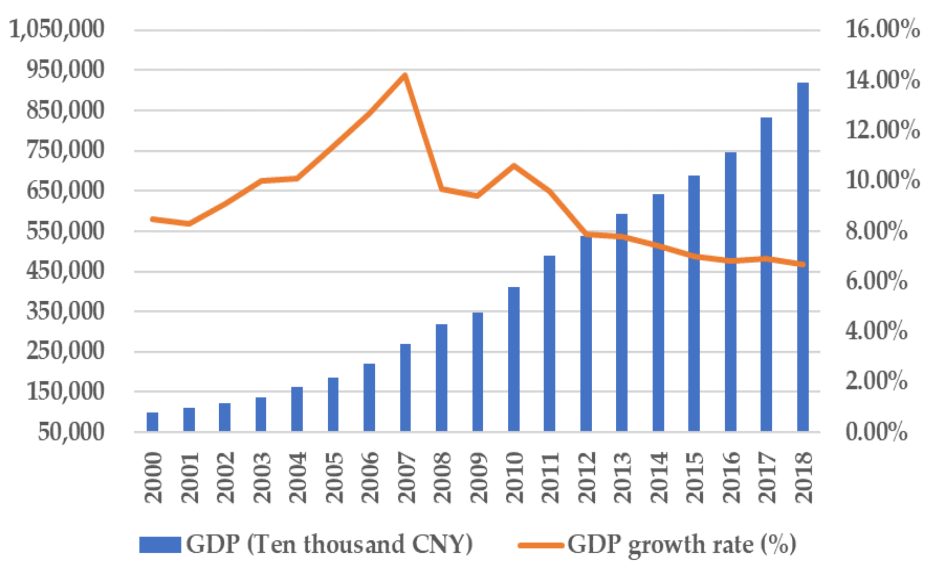
Benefiting from reform and opening itself to the world, China has experienced extensive development and high economic growth (Figure 1), leading to remarkable achievements and significant contributions to the world’s economic development in recent decades. However, its past mode of growth is unsustainable and relies heavily on the massive input of resources, which is not desirable for the long term and emits significant amounts of polluting emissions [1]. Being different from extensive development, high-quality development has become fundamentally requisite for the Chinese government in making determinations concerning development ideas, formulating economic policy, and implementing macro-control in the present and future [2,3]. It is necessary to accelerate the formation of index, policy, standard, and statistical systems, performance evaluations, and performance appraisals to promote high-quality development. High-quality development alone can meet China’s growing lifestyle demands; additionally, it embodies China’s new conceptualization of development (with reference to the “five development concepts” of China, which includes innovative development, coordinated development, green development, open development, and shared development), in which it aims to promote efficient, dynamic change to achieve development that is fairer, safer, higher quality, and more efficient and sustainable. We note that high-quality development in China is defined as that where innovation becomes the primary driver, coordination becomes the intrinsic characteristic, green becomes the universal form, open becomes the necessary way, and sharing becomes the fundamental goal [4,5].
It is obvious that improving efficiency and TFP is key to high-quality development, as they are indeed the implicit requirements of it. In our study, we assume the following definition for high-quality development efficiency: that in which an economy can not only maximize GDP and minimize environmental consequences (nongreen development) under specific input conditions for labor, capital, energy, and other factors, but also optimize innovation, coordination, open, and sharing developments, this to be ideal, and expandable, in general, to economic development efficiency and, in particular, green economic development efficiency. Therefore, we seek to understand how to better evaluate high-quality development efficiency and TFP for regional economies in China. What are the characteristics of spatial trends and spatial-temporal correlation pattern of the high-quality development efficiency and TFP of regional economies in China? What are the factors influencing the high-quality development efficiency and TFP of regional economies in China? It has the important theoretical and practical significance to clarify and solve these problems.
The purpose of our study is to evaluate the high-quality development efficiency and TFP of regional economies in China from 2000 to 2018 and to explore the characteristics of spatial-temporal pattern evolution and its influencing factors. To the best of our knowledge, this is the first paper to study China’s high-quality development efficiency and TFP from the perspectives of the five development concepts. The main contributions of our study are as follows: First, the static high-quality development efficiency and dynamic high-quality development TFP of regional economies in China are evaluated by using the SBM-DDF model based on undesirable output, and our study expands the research perspective. Second, our study identifies the spatial trends and spatial-temporal correlation pattern of high-quality development efficiency and TFP by using the ESDA model, providing evidence for the spatial heterogeneity, imbalance, and correlation of high-quality development efficiency and TFP of regional economies in China. Third, our study utilizes the Tobit model to explore the influencing factors of high-quality development efficiency and TFP, which is very beneficial in terms of policy implications. The inferences obtained from our study not only are helpful for government managers and policymakers concerned with high-quality development but also provide clearer pictures of different provinces in China and may assist in under the scenario from a broader and more inclusive regional angle. This study has important academic and practical application value for high-quality development research in China as well as other countries or regions.
The rest of this paper is organized as follows: Section 2 summarizes in detail the literature review about high-quality development efficiency at home and abroad. Section 3 briefly introduces some materials and methods. Section 4 presents the results, including the evaluation of high-quality development efficiency and TFP of regional economies in China, and spatial trends, spatial-temporal correlation patterns and the influential factors of high-quality development efficiency and TFP. Some discussions are given in Section 5. Some conclusions with summaries and policy recommendations, main contributions, limitations, and future research possibilities are drawn in Section 6.
2. Literature Review
At present, the research on high-quality development mostly focuses on the connotations [6], characteristics [7,8] and countermeasures of high-quality development [9,10]. Research on the definition of high-quality development can be summarized into the following three categories: the first category considers high-quality development to be high-efficiency, fair, green sustainable development aiming at meeting people’s growing needs for a better life; the second category emphasizes the transformation from high speed to high quality in high-quality development; and the third category considers high-quality development to include the process of social reproduction and the all processes in social and economic life. However, in view of different scholars’ different understandings of high-quality development, there is still a lack of consistency in evaluations of high-quality development in academic circles, and a unified evaluation index system has not yet been formed. The evaluation of high-quality development is still in its infancy and remains to be further explored, especially for high-quality development efficiency and TFP.
The common evaluation methods of high-quality development efficiency include single-index evaluation or multi-index weighted combination scoring evaluation. For example, some scholars use the investment efficiency, labor productivity growth, intermediate input-output rate of enterprises and other indicators to measure development efficiency. Although these single indicators have certain effects, they have greater one-sided and limitations, and cannot comprehensively reveal the whole picture of a high-quality development level in a certain region. Therefore, the comprehensive evaluation of high-quality development levels through the construction of measurement systems has become a research hotspot in recent years. The evaluation perspectives of these measurement systems are rich and diverse, and the measurement indicators have their own characteristics, which improves the limitations of using a single indicator to represent the high-quality development level [7,10]. For example, Wei et al. [7] constructed a measurement system of high-quality economic development level from the perspectives of economic structure optimization, innovation-driven development, efficient resource allocation, perfect market mechanism, stable economic growth, regional coordination and sharing, high-quality products and services, infrastructure improvement, ecological civilization construction and economic achievements benefiting the people and then used the entropy weight TOPSIS method to measure the high-quality development efficiency of 30 provinces in China. Ma et al. [11] constructed a high-quality development index system from the perspectives of high-quality supply, high-quality demand, development efficiency, economic operation and opening-up and measured China’s high-quality development efficiency with the linear weighting method. Wang et al. [12] constructed a high-quality development evaluation system from the perspectives of the main elements, service and regulatory elements, incentives, safety assurance capability, urban credit system, innovation ability, satisfaction degree of citizens, policy environment, economic development environment, legal environment and cultural environment. Wang et al. [13] measured the China’s high-quality development efficiency based on economic vitality, development potential, urban and rural joint forces and ecological strength. Guided by the “five development concepts”, Lv et al. [14] measured the high-quality development level of each province in China in each period and the regional gap between different regions by constructing a high-quality development index evaluation system based on economic vitality, innovation-driven, coordinated development, green development, open development and achievement sharing. Shi et al. [15] and Sun et al. [16] constructed a high-quality development evaluation system including innovation, coordination, green, open and sharing to measure high-quality development efficiency in China. It is worth noting that Chinese government officials and a growing number of scholars believe that high-quality development is based on the “five development concepts”, that is, innovation, coordination, green, openness and sharing are indispensable, which has gradually become the mainstream of evaluating high-quality development.
The evaluation of TFP is one of the most effective calculation methods of high-quality development efficiency, considering that single-index evaluation or multi-index weighted combination scoring evaluation may ignore the internal logic of high-quality development. The data envelopment analysis (DEA) [17,18] model is the main method used for measuring economic development efficiency and TFP, which only requires inputs and outputs to be quantified with no hypothesis function form [19,20], including radial DEA [21,22], oriented DEA [23], original constant return to scale DEA (CCR-DEA) [24], network DEA [25], super-DEA [26], multistage DEA [27,28], SBM [29] and so on. In high-quality development, resources and the environment are not only endogenous variables of economic development but also rigid constraints on the scale and speed of economic development. In the past, GDP was the main evaluation performance of extensive and unsustainable development with massive input, which only considered good outputs, but not the constraint of inputs and bad outputs. It is obvious that even if the economic development level of a certain region is relatively high, if the input is relatively large, it is actually achieved by obtaining resources and sacrificing the development of other regions. From the perspective of the whole society, resources have not been reasonably allocated, and the input-output rate is not high, reducing the TFPof the whole society. The measurement of economic development efficiency can avoid the problem and reflect the input-output efficiency relatively accurately. However, traditional TFP only considers the input constraints of production factors, such as labor and capital, but does not consider the constraints of resources and the environment, which distorts the evaluation of social welfare changes and economic performance, thus misleading policy recommendations. Therefore, a large number of scholars focus on the efficiency of green development. For example, Gökgöz et al. [26] empirically confirmed the substitution effect of renewable energy for energy imports and benchmarked the performance of the selected European Union countries in renewable energy efficiency and productivity from 2004 to 2014 with the perspective of energy security using the superefficiency model of data envelopment analysis. They found that, while Sweden, Germany, Spain, Belgium and Romania were among the efficiency leaders, conventional energy producers limited renewable energy in France and the United Kingdom, and the average TFP of the group increased by 8.4% annually, where technological change (innovation) was the prime driver of productivity growth. Bigerna et al. [30] analyzed the relationship between energy efficiency and the stringency of the environment in 19 European Union countries from 2006 to 2014 with two-stages DEA, decomposing the environmental policy stringency index, OECD regulatory indicators and TFP growth. They found that the pure and scale efficiency indices are negatively affected by sectorial regulation that positively affected the shift of the technological frontier and that environmental policy negatively affects the shift of the efficient frontier but has a positive effect on the scale efficiency. Yu et al. [31] studied the impact of the spatial agglomeration of foreign direct investment on the green TFP of Chinese cities based on data from 285 Chinese cities from 2003 to 2017. They found that progress in green technology plays an important role in improving urban green TFP and that foreign direct investment plays a positive role in promoting green TFP. Amri [32] examined the linkage between CO2 emissions and TFP as a measure of income, information and communication technology, trade, financial development and energy consumption in Tunisia from 1975 to 2014. They found that trade, financial development and energy consumption negatively affect the environmental quality. Adnan et al. [33] summarized the socioeconomic effects of COVID-19 on various aspects of the world economy and noted that the COVID-19 epidemic checked the resilience of the agricultural sector in Malaysia, especially the paddy industry. The above studies have important reference value, but the measurement of high-quality development efficiency and TFP from the perspective of five development concepts needs to be further studied.
3. Materials and Methods
First, to evaluate the high-quality development efficiency and TFP, the SBM-DDF model combined with high quality development is introduced in detail in Section 3.1. In addition, the spatial autocorrelation model, including the trend surface model, the global Moran’s I index the local Moran’s I index, are given in Section 3.2. Furthermore, the Tobit model for influencing factors of high-quality development efficiency and TFP is constructed in Section 3.3. Finally, the indicators for evaluation and data sources are discussed in Section 3.4 and Section 3.5, respectively.
3.1. The Evaluation with SBM-DDF Model
When there are excessive inputs or insufficient outputs, that is, the nonzero relaxation of inputs or outputs, the radial DEA will overestimate the efficiency of the evaluation object, and the oriented DEA may not be accurate due to neglecting a certain aspect of inputs or outputs. Traditional DEA assumes that all the outputs should be maximized for the given input level. However, when undesirable outputs are generated as byproducts of desirable outputs, the assumption is no longer appropriate [34]. It should be noted that network DEA and multistage DEA may not be suitable for the evaluation of high-quality development efficiency proposed in our study, considering that the five developments are synchronous and equally important. In the different deformations of DEA, the direction distance function (DDF) is one of the most popular models, which considers the effects of desirable and undesirable outputs separately and can help increase the desirable output and reduce the undesirable output simultaneously [35]. The slacks-based measure (SBM) model contains slacks variables of input and output, which can prevent DDF models’ radial character and directivity from being effectively avoided. To overcome these defects, the slacks-based measure of directional distance functions (SBM-DDF) model is developed by minimizing the ratio of the average undesirable output reduction to the average desirable output increment [36,37]. The nonradial model is generally treated as a composite index for modeling economic environmental performance. The SBM-DDF model has been widely used in the evaluation of TFP because it decreases undesirable outputs while increasing the desirable outputs at the same time [38,39,40]. The essence of high-quality development efficiency is to investigate how to produce better outputs and fewer bad outputs under some inputs, which needs to be measured and decomposed under the framework of TFP. In other words, the SBM-DDF model can achieve more accurate measurements of high-quality development efficiency and TFP compared with other methods.
Many studies show that the SBM-DDF method based on the slacks variable and Luenberger productivity indicator best fits the context of the regional economy in terms of measuring TFP [38], which has gained popularity in academia both at home and abroad. A province is represented as with inputs , desirable outputs and undesirable outputs . The global production possibilities set of high-quality development, emphasizing the consistency and comparability of the production frontier [38]:
where denotes the weight of each cross section, the two constraints are that the sum of the weight variables is 1 and that nonnegative weight variables represent production technology as the variable return to scale (VRS) [41]; if the constraint that the sum of weight variables is 1 is removed, it means constant return to scale (CRS) [42]. In this paper, the high-quality development efficiency calculated under the CRS condition is recorded as HQE(CRS), and the high-quality development efficiency calculated under the VRS condition is recorded as HQE(VRS).
Drawing on the experience of Fukuyama and Weber [38,39,43,44], we define the SBM-DDF that covers undesirable outputs considering high-quality development as follows:
where denote the vectors of inputs, desirable outputs and undesirable outputs, respectively. denote the direction vectors for decreasing inputs, increasing desirable outputs and decreasing undesirable outputs, respectively. denote the slacks vectors for redundant inputs, inadequate desirable outputs and redundant undesirable outputs, respectively.
The Luenberger productivity indicator is more suitable for measuring the TFP, which considers the decrease in inputs and increase in outputs simultaneously, avoiding different perspectives and the rate variable [45,46]. The Luenberger productivity indicator between period and period is calculated as follows [38]:
In addition, the Luenberger productivity index can be divided into HQPEC, HQPTP, HQSEC, and HQTPSC [38,39].
where HQPEC represents the catching-up effect, which measures the maximum closeness degree of the practical production of a DMU to the production frontier; HQPTP represents the progress or retrogress of technology, which measures the movement of the production frontier from period to ; HQSEC represents the scale effect caused by the change of efficiency value, which measures the change of scale efficiency; and HQTPSC represents the scale effect of technology development [47,48].
3.2. Spatial Autocorrelation Model
The trend surface is the nearsighted value of the actual surface. By abstracting the mathematical surface and filtering out the influence of local random factors, it can accurately simulate the spatial distribution law of geographical elements, show the change trend of geographical elements in the regional space and be used to explore the overall spatial layout characteristics of high-quality development efficiency and TFP of regional economies in China [48,49]. It is assumed that is the actual level of high-quality development efficiency orTFP, which represents the spatial plane coordinates. The trend surface model is defined as follows [50]:
where is the trend function, which represents the fitting value of the high-quality development efficiency or TFP trend surface in the region, reflecting the macro distribution law of HQE or HQTFP; is the autocorrelation random error, which represents the error between the real value and trend value of HQE or HQTFP in the region , namely the influence of random factors. Based on previous research experience, this paper uses common second-order polynomials to measure the trend value of HQE or HQTFP of regional economies in China. The trend function can be expressed as [51]:
where are regression fitting coefficients of trend function, respectively.
The theory of spatial econometrics holds that the observation value of an attribute on a geospatial unit is closely related to the observation value on the adjacent space unit, and there is a spatial autocorrelation characteristic. The exploratory spatial data analysis (ESDA) model can reveal spatial autocorrelation characteristics and spatial interactions by calculating the global and local Moran’s I indices of different attribute values of different spatial units. The global Moran’s I index of high-quality development efficiency and TFP is calculated as follows [52,53]:
where represents the HQE or HQTFP and represents the normalized spatial weight matrix; Moran’s I index ranges from [−1, 1]; if the value of Moran’s I index is less than 0, the HQE or HQTFP is negatively correlated; if the value of Moran’s I index is greater than 0, the HQE or HQTFP is positively correlated; if the value of Moran’s I index equals 0, the HQE or HQTFP is irrelevant. Standardized statistics are usually used to test the significance of the global Moran’s I index. The formulas are shown as follows [53,54]:
If the value of Z is significant and positive, it indicates that there is a positive spatial autocorrelation between the HQE or HQTFP. If the value of Z is significant and negative, it indicates that there is a negative spatial autocorrelation between the HQE or HQTFP. If the value of Z equals 0, it indicates that the HQE or HQTFP presents a random distribution state.
The local distribution of the spatial correlation of high-quality development efficiency and TFP among regions may appear “atypical”, which cannot be reflected by the global indicators. Therefore, it is necessary to use the local indicator of spatial correlation (LISA), i.e., local Moran’s I index, to analyze the local characteristics of HQE or HQTFP correlations among regions. The calculation formula is as follows [55]:
The index measures the degree of correlation between the regions and their surrounding regions: if the value of is positive, it indicates the High–High (H-H) or Low–Low (L-L) of the HQE or HQTFP autocorrelation type. If the value of is negative, it means Low–High (L-H) or High–Low (H-L) of the HQE or HQTFP autocorrelation type. High–High (H-H) type indicates that the HQE or HQTFP of the current region and the surrounding regions are similar and relatively high, and there is a smaller difference in spatial difference. The Low–High (L-H) type means that the HQE or HQTFP of the current region is relatively low, but HQE or HQTFP of its surrounding regions are generally higher, there is a relatively large difference in spatial difference. The Low–Low (L-L) type indicates that the HQE or HQTFP of the current region and its surrounding regions are similar and relatively low; there is a small difference in spatial difference. The High–Low (H-L) type means that the HQE or HQTFP of the current region is relatively high, and the HQE or HQTFP of its surrounding regions are generally lower; there is a larger difference in spatial difference [56].
3.3. Tobit Model for Influencing Factors
Considering the data structure and attributes of HQE and HQTFP, using the ordinary least squares (OLS) model may cause bias and inappropriate parameter estimation. Based on previous research experience, the Tobit model is used to estimate the influencing factors of high-quality development efficiency and TFP in this paper. We set up the Tobit model as follows [57,58]:
where represents the HQE(CRS), HQE(VRS), HQTFP, HQPEC, HQPTP, HQSEC, and HQTPSC, respectively. is the independent variable vector; is the intercept term vector; is the correlation coefficient vector, and is the random error term. Based on previous research experience, in this paper, the independent variables include the role of government (GOV), marketization level (MAR), urbanization rate (URB), financial development (FIN), infrastructure (INF), endowment structure (END), and foreign direct investment (FDI).
3.4. Indicators for Evaluation
Based on the connotation of high-quality development and “five development concepts”, this paper measures high-quality development efficiency and TFP based on the SBM-DDF model including input indicators (labor, financial capital, human capital, and energy), desirable outputs (economic development, innovation development, coordinated development, shared development, and open development), and undesirable outputs (nongreen development). Based on the principle of availability, comparability, and continuity of statistical data, learning from predecessors’ experience [59,60,61], the evaluation indicator system and influencing variables of high-quality development efficiency and TFP in this paper are shown in Table 1.
3.5. Data Sources
The current research objective does not include the empirical analysis of Hong Kong, Macao, or Taiwan because of the special endowment and data availability. The 31 areas are divided into four regions, eastern, central, western, and northeast, according to the distribution of natural resources and the level of economic and social development of China’s provincial administrative regions. The specific division results are shown in Table 2.
Relevant data from 2000 to 2018 are selected using the China Statistical Yearbook, China Environmental Yearbook, China Energy Statistics Yearbook and Statistical Yearbooks of Provinces. Considering that the data of the capital stock of provinces in China cannot be obtained from the statistical yearbook, most existing literature uses the formula to calculate capital stock. and are the capital stock at periods and , respectively. denotes investment and is the depreciation rate at period . In this paper, the indices of currency value are used to eliminate the effect of price fluctuation through the relevant price indices. Table 3 summarizes the descriptive statistics of the raw data of each variable observed for 31 DMUs.
4. Results
First, the high-quality development efficiency and TFP of regional economies in China are evaluated in Section 4.1. In addition, to further explore the spatial-temporal pattern evolution characteristics, the spatial trends and spatial correlation pattern of high-quality development efficiency and TFP are studied in Section 4.2 and Section 4.3 from the spatial perspective of economic geography, respectively. Furthermore, the influential factors of high-quality development efficiency and TFP are discussed in Section 4.4.
4.1. The Evaluation on High-Quality Development Efficiency and TFP
In this subsection, the high-quality development efficiency and TFP are measured based on the SBM-DDF model with Maxdea software from 2000 to 2018, and the average values of the results are shown in Table 4. Table 4 contains seven headings: HQE(CRS), HQE(VRS), HQTFP, HQPEC, HQPTP, HQSEC, and HQTPSC, which are employed to analyze the high-quality development efficiency and TFP of regional economies in China from different angles.
High-quality development efficiency (HQE) measures the relative relationship between provinces and production boundaries in a given period, and is a static analysis. From Table 4, we can find that the average value of the nationwide high-quality development efficiency under CRS from 2001 to 2018 is 0.4320, and the average value of the nationwide high-quality development efficiency under VRS is 0.5971. The average values of HQE(VRS) are slightly higher than those of HQE(CRS). From the perspective of different regions, the high-quality development efficiency under CRS of the eastern region (0.7392) is the highest, while the high-quality development efficiency under CRS is the lowest in the central region (0.2141). The high-quality development efficiency under VRS of the eastern region (0.8220) is also the highest, followed by the northeast region (0.7521), the western region (0.5217), and the central region (0.2952). From the perspective of various provinces, only Guangdong, Shanghai, Jiangsu, and Tibet are on the production boundary of high-quality development efficiency, and other provinces are not. The provinces with higher efficiency are concentrated in the eastern region. The provinces with lower high-quality development efficiency are Yunnan, Guizhou, Guangxi, Henan, Shanxi, and Gansu. It is worth noting that Tibet’s high-quality development efficiency benefits from its lower inputs, which produces a moderate amount of good outputs and a small amount of bad outputs. It shows that high-quality development is not “more input and more output”, but “less input and better output” from the side.
High-quality development TFP (HQTFP) analysis is a dynamic method that can analyze the relative position change (efficiency change) of each province and the production boundary, and the movement of the production boundary (technical progress). The average growth rate of the HQTFP nationwide in regional economies in China from 2001 to 2018 is 2.83%. From the perspective of decomposition of HQTFP, the average growth rate of the HQPTP nationwide is the largest at 3.06%, followed by HQPEC at 0.85%. However, the average growth rates of HQSEC and HQTPSC nationwide are negative, at −0.29% and −0.79%, respectively. From the perspective of different regions, the average growth rate of the HQTFP in the eastern region is the largest at 3.93%, which is determined by the HQPTP (4.07%) and HQTPSC (0.62%). The average growth rate of the HQTFP in the central region is lowest at 0.54%, which is determined by the HQPTP (2.64%) and HQSEC (0.73%). From the perspective of various provinces, in addition to Anhui, Fujian, Jiangxi, Hainan, and Tibet, the HQTFP of other provinces shows positive growth. The top three fastest growth rates of HQTFP are Sichuan (11.28%), Shandong (8.88%), and Qinghai (8.20%). The last three slowest growth rates of HQTFP are Hainan (−5.28%), Jiangxi (−3.23%), and Tibet (−0.76%). Only Beijing, Tianjin, and Zhejiang have positive HQTFP, HQPEC, HQPTP, HQSEC, and HQTPSC, where the TFP of high-quality development is driven by pure efficiency change, pure technological progress, scale efficiency change, and technological scale change at the same time.
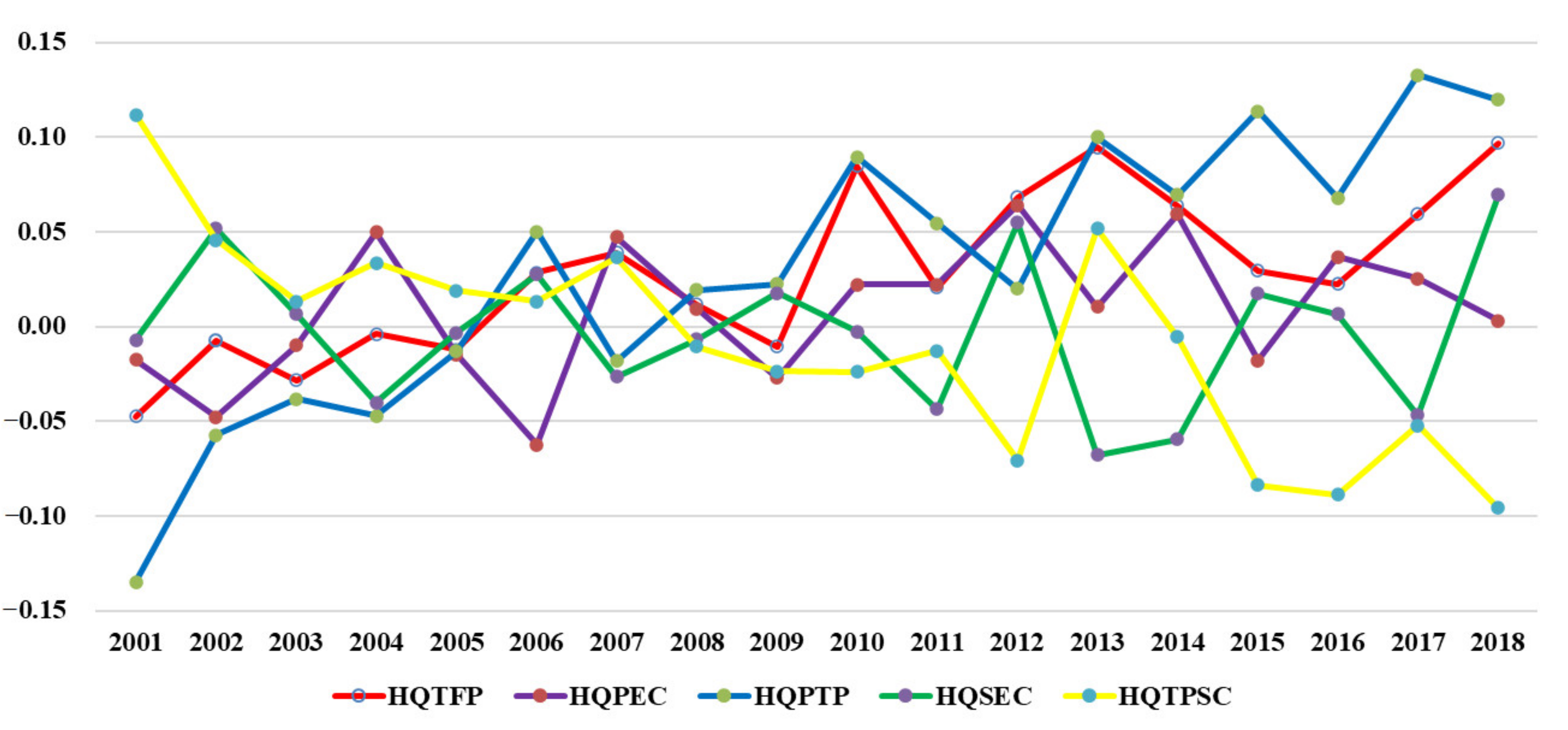
The trend of HQTFP and its decomposition of regional economies in China with regard to time from 2001 to 2018 are shown in Figure 2, wherein the horizontal axis represents the year and the vertical axis represents the efficiency value. Figure 2 shows that from 2001 to 2018, HQTFP shows a fluctuating rising trend overall. In 2010, there was a significant increase led by the HQPTP and HQPEC. It is not difficult to determine that the HQPTP has increased at a similar pace as the HQTFP in the past twenty years. The contribution rates of HQPEC and HQSEC fluctuate irregularly. The contribution of HQTPSC shows a downward trend, which deserves our attention, and the trend has become more severe in the last five years. HQTPSC has become the largest obstacle of HQTFP, which shows the urgency and great potential of improving the high-quality development TFP of regional economies in China by upgrading technology.
4.2. The Spatial Trends of High-Quality Development Efficiency and TFP
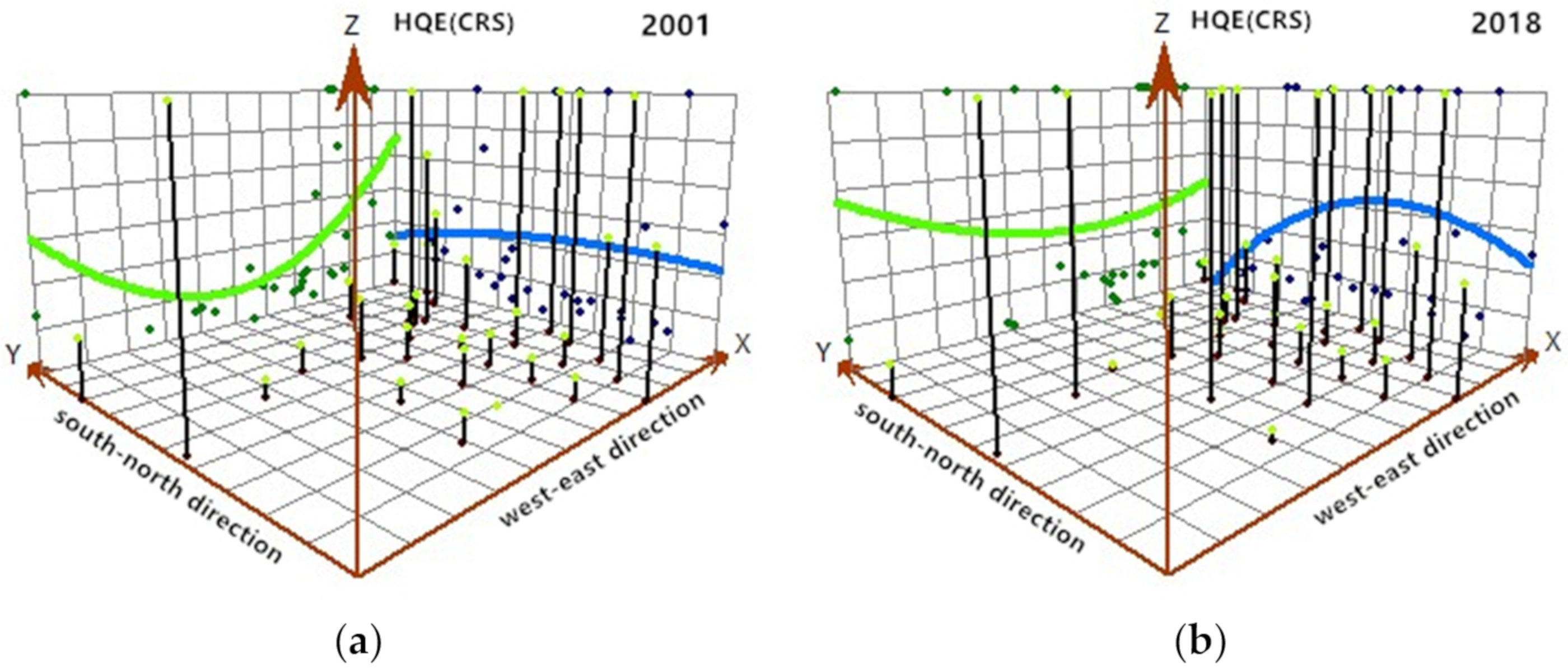
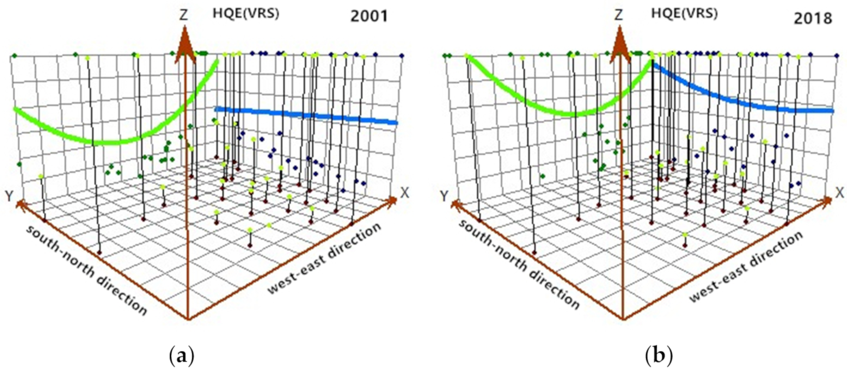
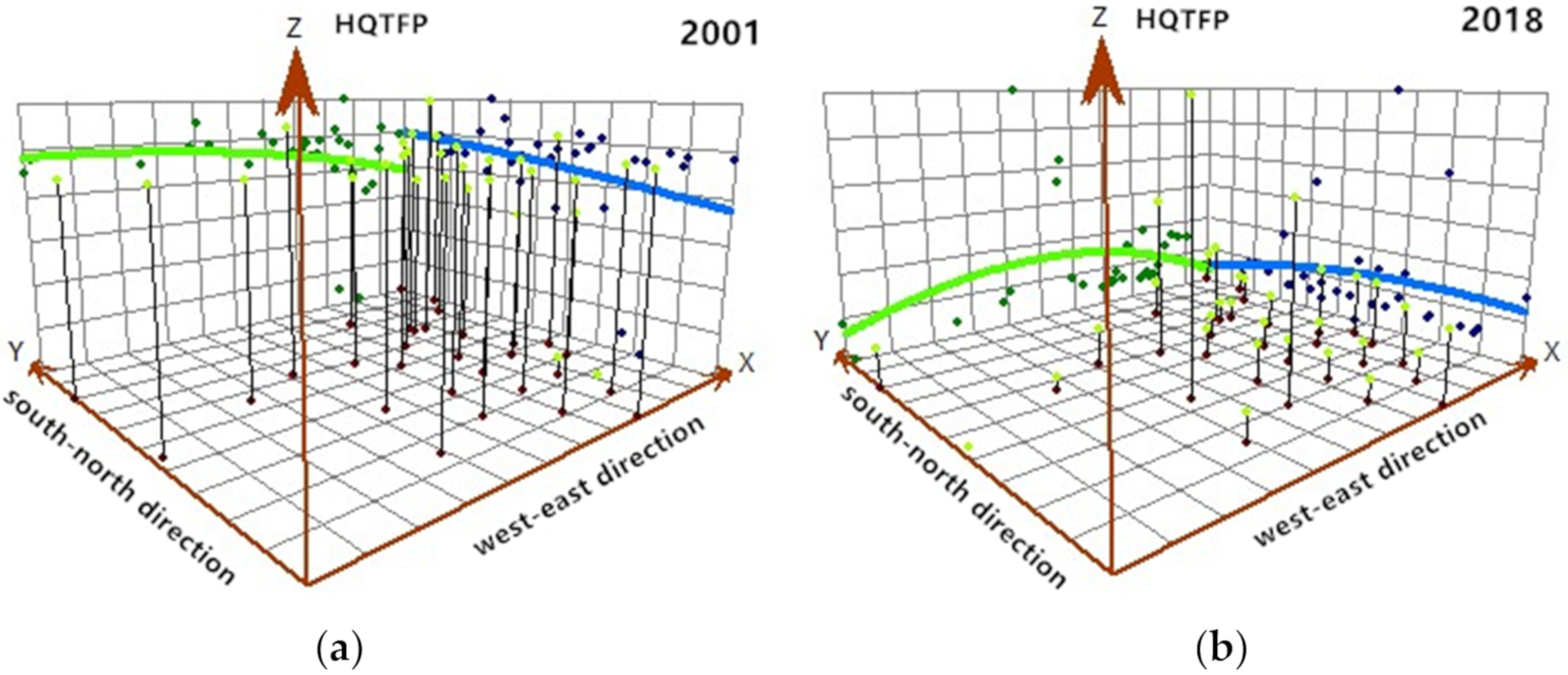
The high-quality development efficiencies among the eastern, central, western, and northeast regions are significantly different from those in Table 4. To further understand the differences, the spatial distribution tendency of the high-quality development efficiency of regional economies in China in 2001 and 2018 is visually described by using the tendency analysis tool of ArcGIS 10.6 software (ESRI, Redlands, CA, USA) from the American ESRI Company. As shown in Figure 3, Figure 4 and Figure 5, the Z axis represents the value of regional high-quality development efficiency, the X axis is the west–east direction, and the Y axis is the south–north direction. For high-quality development efficiency, the U and inverted-U trend lines show that HQE(CRS) and HQE(VRS) have significant regional differences in the east–west direction, presenting a significant feature of spatial imbalance. The high-quality development efficiency of the eastern region is higher than that of the western region. In the south–north direction, there is little difference among the HQE(CRS), and the HQE(VRS) of the southern region is higher than that of the northern region in 2001; the result is opposite in 2018. For the high-quality development TFP, the eastern region is slightly higher than that of the western region, and the northern region is slightly higher than that of the southern region in 2018.
4.3. The Spatial Correlation Pattern of High-Quality Development Efficiency and TFP
“The first law of geography” holds that everything is related to each other, and there is a certain spatial correlation between them. The global spatial correlation of the high-quality development efficiency and high-quality development TFP in regional economies in China from 2001 to 2018 are calculated using ArcGIS 10.6 software. The results of the global Moran’s I index are shown in Table 5. The Moran’s I indices of HQE(CRS) and HQE(VRS) show that there is significant positive spatial autocorrelation in regional economies in China, indicating that the high-quality development efficiency is not completely random, but is the result of positive spatial correlation of high-quality development efficiency. The spatial agglomeration of the high-quality development efficiency in regional economies in China shows a significant spatial dependence. There is only significant positive spatial autocorrelation of HQTFP in regional economies in China in 2001, 2007, 2016, and 2017, indicating that the high-quality development TFP is partially randomly distributed, and the spatial correlation needs to be increased with ongoing high-quality development.
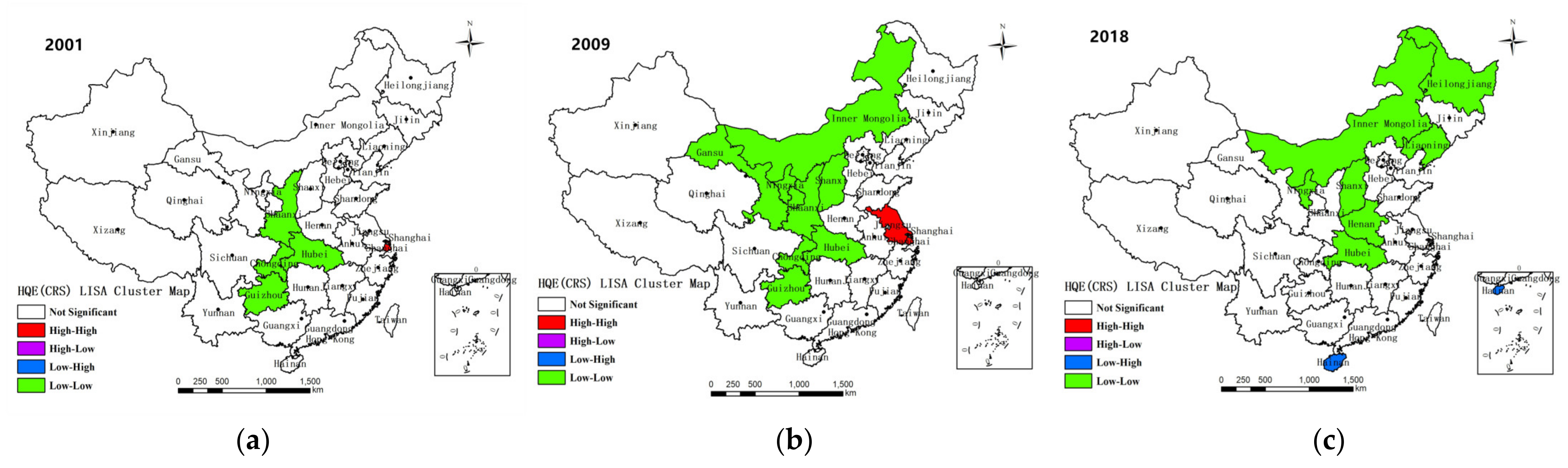
Whereas the global Moran’s I index cannot reveal local spatial correlation and heterogeneity, this paper further tests whether there is local spatial agglomeration of high-quality development efficiency and high-quality development TFP in regional economies in China through the local indicators of spatial association (LISA). The local spatial autocorrelation LISA agglomeration map reflects the local spatial interdependence and spatial heterogeneity of high-quality development efficiency and TFP in regional economies in China. The LISA graphs for 2001, 2009, and 2018 are shown in Figure 6, Figure 7 and Figure 8, which show the clustered points of high-quality development efficiency and TFP, respectively, in regional economies in China, in terms of the four types of spatial correlations: High-High, Low-Low, High-Low, and Low-High.
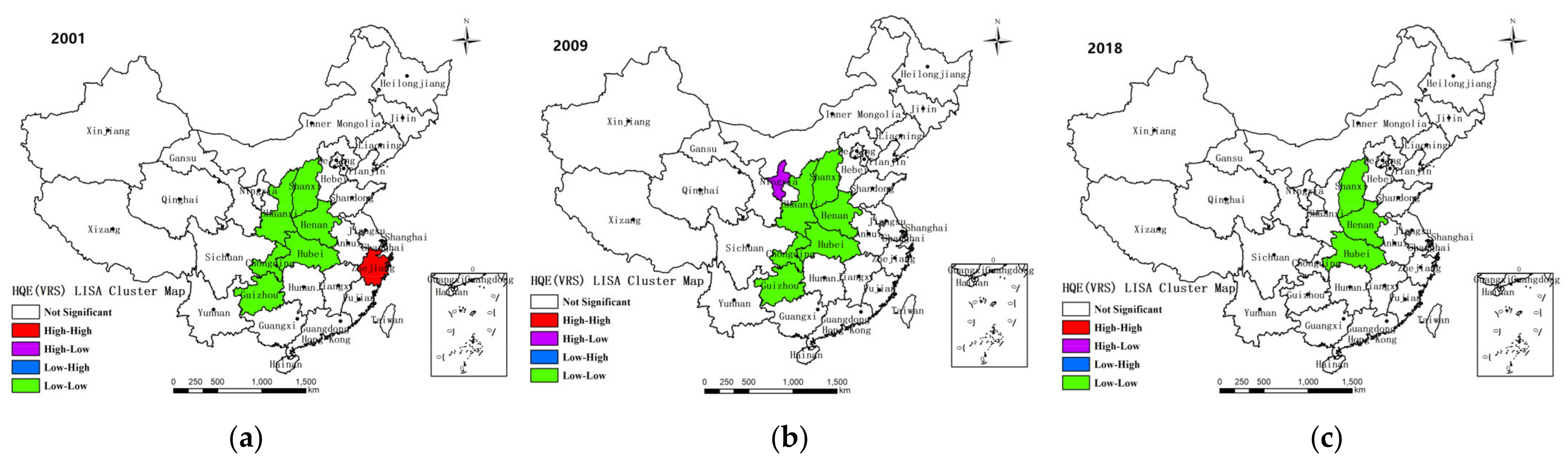
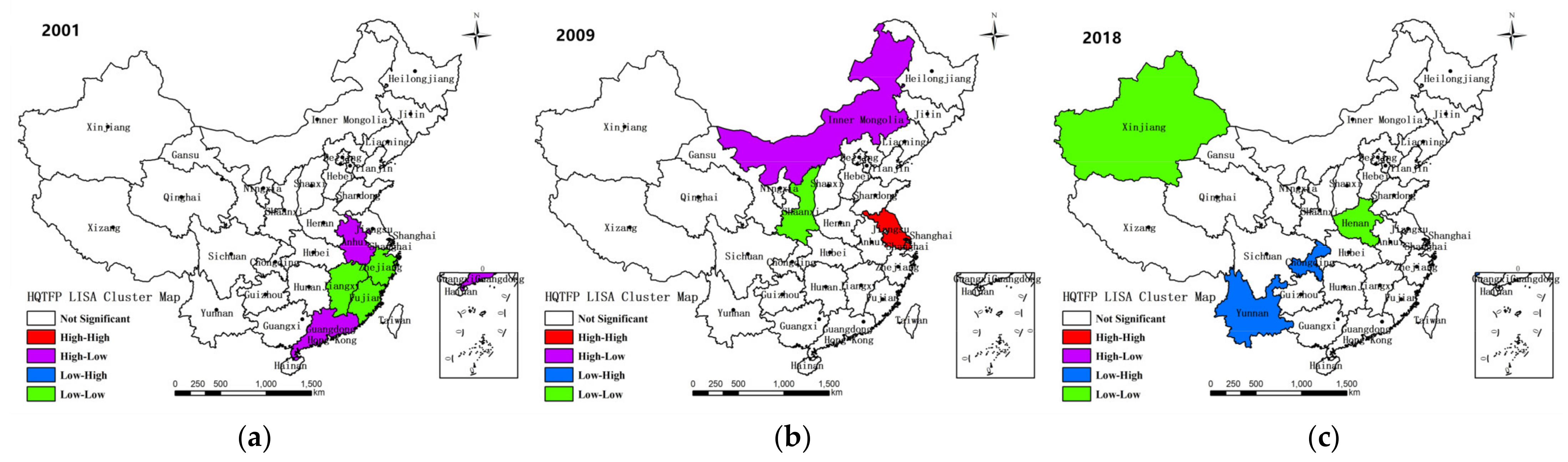
The Chinese regional HQE(CRS) is characterized by the L-L type, as shown in Figure 6. In 2001, only Shanghai belonged to the H-H type, showing a significant positive spatial correlation. The provinces belonging to the L-L type were mainly located in Shannxi, Hubei, Chongqing, and Guizhou. Furthermore, there was no province that belongs to the H-L and L-H types. In 2009, the provinces of the H-H type extended to Shanghai and Jiangsu, and the provinces of the L-L type expanded northward to Ningxia, Shanxi, Gansu, and Inner Mongolia, including Shannxi, Hubei, Chongqing, and Guizhou. In 2018, the provinces of the L-L type adjusted northeastward to Hubei, Henan, Shanxi, Ningxia, Inner Mongolia, Liaoning, and Heilongjiang. The main reason may be that these provinces tend to use larger amounts of material inputs to obtain greater economic benefits. Such extensive development led to higher bad outputs and imbalance. It was worth noting that Hainan evolved into the L-H type. The Chinese regional HQE(VRS) was also characterized by the L-L type, mainly shown in Figure 7. In 2001, only Zhejiang belonged to the H-H type, and there were six provinces belonging to the L-L type, including Shanxi, Shannxi, Henan, Hubei, Chongqing, and Guizhou. Similarly, there was also no province that belonged to the H-L and L-H types. In 2009, Ningxia evolved into H-L type. In 2018, the provinces of the L-L type reduced to Hubei, Henan, and Shanxi. Compared with HQE(CRS) and HQE(VRS), the type of HQTFP was obviously different from Figure 8. In 2001, only Zhejiang, Jiangxi, and Fujian belonged to the L-L type, and Guangdong and Anhui belonged to the H-L type. There was no province that belonged to the H-H and L-H types. In 2009, Shanghai and Jiangsu evolved into the H-H type, Shannxi evolved into the L-L type, and Inner Mongolia evolved into the H-L type. In 2018, Chongqing and Yunnan evolved into the L-H type, whereas provinces with low scores more easily accepted efficient production models. Henan and Xinjiang evolved into the L-L type. Overall, there is a long way to go from extensive development to high-quality development, so different types of local agglomerations will coexist in the future.
4.4. Influential Factors of High-Quality Development Efficiency and TFP
In this subsection, first, Phillips–Perron (PP) and augmented Dickey–Fuller (ADF) unit root test results show that the series are not order-one integrated. After the first-order difference processing, all the sequences in this study meet the 10% significance level of rejection of the original hypothesis, and the panel data are stationary series, so further cointegration tests are needed. Both Pedroni and Kao cointegration tests meet the 10% level, and there is a significant cointegration relationship between the data, meaning that the data are suitable for empirical analysis. Furthermore, the Hausman test shows that the fixed effect model should be selected for the regression analysis. Calculations are carried out in Tobit with Eviews 8 software, and Table 6 shows the regression analysis results. Under the two hypotheses of CRS and VRS, the influence direction of each factor on high-quality development efficiency is basically the same. The influence direction of each factor on high-quality development TFP is also basically the same.
The empirical results show that GOV and URB have a positive and significant impact on HQE(CRS), HQE(VRS), HQTFP, HQPEC, HQPTP, HQSEC, and HQTPSC with a significance level of 1%, indicating that the role of government and urbanization rate can improve the high-quality development efficiency and TFP. In other words, the higher the proportion of fiscal expenditure to GDP and the proportion of urban population in the total population, the higher the value of the high-quality development efficiency and TFP. The coefficients of MAR are positive and significant on HQE(CRS), HQTFP, HQPEC, HQPTP, HQSEC, and HQTPSC with a significance level of 1%, except for HQE(VRS) with a negative but nonsignificant coefficient. It is not difficult to determine that the marketization level has the largest impact on the high-quality development efficiency and TFP, implying that the increase in the efficiency and productivity depends largely on the improvement of the marketization level; that is to say, the proportion of nonstate-owned fixed assets investment makes the most important contribution to the high-quality development efficiency and TFP. Concerning the impact of the other control variables, FIN, INF, and FDI have a positive and significant impact on HQE(CRS) and HQE(VRS) and a negative and significant impact on HQTFP, HQPEC, HQPTP, HQSEC, and HQTPSC, indicating that financial development, infrastructure, and foreign direct investment can improve high-quality development efficiency, but can also reduce high-quality development TFP. The main reason can be explained as follows: the improvement of financial efficiency is conducive to the improvement of high-quality development efficiency, but the rapid expansion of financial scale reduces the high-quality development TFP. Furthermore, with the continuous improvement of infrastructure, the outflow of regional factors may be accelerated, which is not conducive to the improvement of high-quality development TFP. It is worth noting that FDI can bring advanced enterprise management experience and cutting-edge technology, which promotes the improvement of high-quality development efficiency. However, the “pollution paradise” hypothesis holds that the level of environmental regulation in developed countries is higher than that in developing countries. Therefore, there must be a large amount of FDI flowing into the pollution intensive sectors of developing countries. Considering that foreign-funded enterprises tend to migrate polluting enterprises to developing countries, it is not conducive to the promotion of high-quality development TFP, in contrary, it will have a certain inhibitory effect on high-quality development TFP. It is worth noting that END has a negative and significant impact on HQE(CRS), HQE(VRS), HQTFP, HQPEC, HQPTP, HQSEC, and HQTPSC, which is consistent with our expectation. If the capital labor ratio increases, it shows that the economic structure is transforming from labor-intensive to capital-intensive. Capital-intensive industries and labor-intensive industries tend to be heavy-pollution industries and light-pollution industries, respectively.
5. Discussion
In this section, a discussion comparing these findings with those of previous studies is presented in two parts. The first part relates to the indicators of high-quality development, and the second part describes the evaluation of high-quality development TFP.
5.1. Indicators of High-Quality Development
The classification of a high-quality development index system is mainly based on the connotation of high-quality development. Different understandings of the connotation lead to different measurement index systems. Generally, the measurement of high-quality development mainly focuses on the following three aspects: (i) from the five development concepts guiding high-quality development, that is, to build the high-quality development evaluation index system from the five fields of innovation, coordination, green, open, and sharing [14,15]; (ii) from the characteristics of high-quality development, that is, from the five areas of high-quality supply, high-quality demand, high-quality input-output, high-quality income distribution, and high-quality economic cycle to build the high-quality development evaluation index system [7,11]; and (iii) from the requirements of high-quality development, that is, to build the high-quality development evaluation index system from the three areas of quality change, efficiency change, and dynamic change [12,13]. The results of different index measurement systems are slightly different. Of course, the above three measurement index systems of high-quality development are also suitable for other countries or regions. Considering the internal or external factors of different countries or regions, the index systems may be slightly different. For the new concept of high-quality development, scholars at home and abroad need to make efforts to further explore and improve in the future.
5.2. Evaluation on High-Quality Development TFP
Generally, from the perspective of the evaluation index system, high-quality development TFP includes green economic development TFP, to a certain extent. For the evaluation of green economic development TFP, scholars consider not only the good output GDP but also the bad output pollution emissions. For the evaluation of high-quality development TFP, on the one hand, it considers the good output of GDP and the bad output of pollution emissions (nongreen development); on the other hand, it also considers the good outputs innovative development, coordinated development, open development, and shared development. Currently, for the evaluation of economic high-quality development TFP, most scholars focus on the evaluation of green economic development TFP. Li et al. [62] measured the green TFP of the Pearl River Delta urban agglomeration from 2005 to 2018 and analyzed its changes from time and space dimensions by using the SBM Malmquist–Luenberger model. Hou et al. [63] studied the spatial effect and transmission mechanism of market integration on regional green TFP by calculating the Malmquist–Luenburger model based on panel data of 30 provinces in China from 2008 to 2017. Elsadig [64] assessed the impact of green TFP intensity on sustainable productivity growth in Malaysia, Indonesia, the Philippines, Singapore, Thailand, China, Japan, and South Korea. From the perspective of the TFP evaluation method, they have the same usability, but the difference lies in how the index system and model are built from the theoretical level. It should be pointed out that the TFP obtained by different evaluation methods may be different. The focus of this study is not on the innovation of methods but creatively combines the connotation of high-quality development theory with the general SBM model for quantitative analysis. It should be noted that the combination of a high-quality development assessment system with different measurement methods of TFP is also applicable to other countries and regions.
6. Conclusions
6.1. Summaries and Policy Recommendations
In this paper, we first analyze the static high-quality development efficiency and dynamic high-quality development TFP of regional economies in China from 2000 to 2018 with the Malmquist productivity index and the SBM-DDF model based on an undesirable output perspective with slacks-based methods. Then, the spatial trends and spatial correlation pattern of high-quality development efficiency and TFP of regional economies in China are identified. In addition, we explore the influencing factors of high-quality development efficiency and TFP of regional economies in China with the Tobit model. The main research results are as follows:
- (1)
- The high-quality development efficiency of the eastern region is the highest, followed by the northeast region, the western region, and the central region. Only Guangdong, Shanghai, Jiangsu, and Tibet are on the production boundary of high-quality development efficiency. Yunnan, Guizhou, and Guangxi have lower high-quality development efficiency. The average growth rate of the high-quality development TFP in the eastern region is the largest, and that in the central region is the lowest. Only Beijing, Tianjin, and Zhejiang have positive TFP, pure efficiency change, pure technological progress, scale efficiency change, and technological scale change at the same time.
- (2)
- From 2001 to 2018, the high-quality development TFP shows a fluctuating rising trend overall. The U and inverted-U trend lines show that the high-quality development efficiency has significant regional differences in the east–west direction, presenting a significant feature of spatial imbalance. The high-quality development TFP of the eastern regions is slightly higher than that of the western regions, and that of the northern regions is slightly higher than that of the southern regions. There is significant positive spatial autocorrelation in the high-quality development efficiency, which is mainly characterized by the L-L type.
- (3)
- The role of government, urbanization rate, and marketization levels have a positive and significant impact on high-quality development efficiency and TFP. Financial development, infrastructure, and foreign direct investment can improve the high-quality development efficiency but can also reduce high-quality development TFP. The capital–labor ratio has a negative and significant impact on high-quality development efficiency and TFP.
Based on the above research conclusions, we offer some suggestions and advice to government managers and policymakers for improving the high-quality development efficiency and TFP of regional economies in China. First, government managers and policymakers should improve the role of government, urbanization rate, and marketization levels and reduce energy conservation. Second, relying on the spatial characteristics of high-quality development efficiency and TFP, government managers and policymakers should optimize the spatial layout of high-quality development elements to form multilevel, multigradient, dislocation competition, cooperation and win–win high-quality development spatial support systems. Finally, government managers and policymakers also need to take responsibility for adopting a high-quality development path, avoiding extensive development.
6.2. Main Contributions
The main contributions of this paper are as follows: (i) Based on the five development concepts, this paper creatively combines the measurement of TFP of high-quality development with the SBM-DDF model, which not only enriches the theoretical connotation of high-quality development, but also finds one of the effective methods of high-quality development performance evaluation, which is the greatest contribution of this paper. (ii) The results of this paper are helpful to enrich the content of high-quality development research systems from the perspective of spatial economics, and provide an important decision-making reference for the relevant government departments in China to optimize the spatial layout of high-quality development elements and promote the formation of regional spatial patterns with complementary advantages and high-quality development.
6.3. Limitations and Future Research
It needs to be pointed out that the research on high-quality development is still in its infancy; many problems have not been addressed by the academic community, and there are several limitations and future directions of the study presented here. First, we only study one of the three aspects of high-quality development evaluation listed in this paper. The other two different evaluation methods or new evaluation methods will be taken as in-depth theoretical research with technical analysis in the future. Second, due to the lack of data, especially at the micro level, this paper does not include cities or counties in China in the research system. In future work, it will be worth considering the comprehensive measurement of other high-quality development indicators, especially those based on big data from online and offline from different research countries, regions, and geographical levels. Third, in this paper, we carefully use the most common SBM-DDF method to measure the high-quality development efficiency and TFP. There is a need for an improved evaluation system using advanced algorithms, such as SBM-NDEA [65], DNSBM [66], NDDF [67], SFA [68], and panel SFA [69], and the comparison of different methods is worthy of further investigation. Fourth, there may also be more driving paths in the Tobit model as well as potential interactions between them, and further research with more influencing factors, especially the effects of COVID-19, will continue to be interest in the future.
Author Contributions
Conceptualization, X.H. and X.J.; methodology, X.H.; software, X.H.; validation, X.H. and H.L.; formal analysis, X.H.; investigation, X.H.; resources, X.H.; data curation, X.H. and H.L.; writing—original draft preparation, X.H. and H.L.; writing—review and editing, X.H.; visualization, X.H.; supervision, X.H. and X.J.; project administration, X.H. and H.L.; funding acquisition, X.H. and H.L. All authors have read and agreed to the published version of the manuscript.
Funding
This research was funded by the National Natural Science Foundation of China (No. 11871183, No. 61866010, No. 11926349), the Natural Science Foundation of Zhejiang Province (No. LQ19D010001, No. LY18G010018), the Philosophy and Social Science Planning General Project of Zhejiang Province (No. 21NDJC198YB), and the Soft Science Research Program of Zhejiang Province (No. 2019C35010).
Institutional Review Board Statement
Not applicable.
Informed Consent Statement
Not applicable.
Data Availability Statement
The data presented in this study are available from the official website of China Statistical Yearbook (http://www.stats.gov.cn/tjsj/ndsj/, accessed on 30 May 2021) or from the authors.
Acknowledgments
We would like to thank all the anonymous reviewers for their constructive feedback on earlier drafts of this paper.
Conflicts of Interest
The authors declare no conflict of interest.
References
- Zhong, J.; Li, T. Impact of financial development and its spatial spillover effect on green total factor productivity: Evidence from 30 provinces in China. Math. Probl. Eng. 2020, 26, 5741387. [Google Scholar] [CrossRef] [Green Version]
- Gu, W.T.; Wang, J.Y.; Hua, X.Y.; Liu, Z.D. Entrepreneurship and high-quality economic development: Based on the triple bottom line of sustainable development. Int. Entrep. Manag. J. 2020, 17, 1–27. [Google Scholar] [CrossRef]
- Zhang, J.K.; Hou, Y.Z.; Liu, P.L.; He, J.W.; Zhuo, X. The goal and strategic path of high-quality development. Manag. World 2019, 7, 1–7. (In Chinese) [Google Scholar]
- Sun, Y.F.; Ma, A.B.; Su, H.R.; Su, S.L.; Chen, F.; Wang, W.; Weng, M. Does the establishment of development zones really improve industrial land use efficiency? Implications for China’s high-quality development policy. Land Use Policy 2020, 90, 104265. [Google Scholar] [CrossRef]
- Jin, B. Study on the high-quality development economics. China Ind. Econ. 2018, 4, 5–18. (In Chinese) [Google Scholar]
- Jin, P.; Peng, C.; Song, M. Macroeconomic uncertainty, high-level innovation, and urban green development performance in China. China Econ. Rev. 2019, 55, 1–18. [Google Scholar] [CrossRef]
- Wei, M.; Li, S.H. Study on the measurement of economic high-quality development level in China in the new era. J. Quant. Tech. Econ. 2018, 11, 3–20. (In Chinese) [Google Scholar]
- Zhao, A.; Guan, H.; Sun, Z. Understanding high-quality development of marine economy in China: A literature review. Mar. Econ. Manag. 2019, 2, 124–130. [Google Scholar] [CrossRef]
- Chen, Z. A Study on the problems and countermeasures of the development of rural ecotourism in China. J. Adv. Econ. Financ. 2019, 4, 43–47. [Google Scholar] [CrossRef]
- Li, J.C.; Shi, L.M.; Xu, A.T. Discussion on evaluation index system of high-quality development. Stat. Res. 2019, 36, 4–14. (In Chinese) [Google Scholar]
- Ma, R.; Luo, H.; Wang, H.W.; Wang, T.C. Study of evaluating high-quality economic development in Chinese regions. China Soft Sci. 2019, 7, 60–67. (In Chinese) [Google Scholar]
- Wang, S.H.; Mao, C.S. Research on the construction of urban quality development evaluation system from the perspective of macro-quality. In Proceedings of the 5th International Conference on Social Science and Management (ICSSM 2020), Hangzhou, China, 11–12 January 2020; pp. 107–111. [Google Scholar]
- Wang, Q.; Ding, Y.W.; Guo, X.M. Construction of index system for high-quality development of county economy in China. Soft Sci. 2021, 35, 115–119. (In Chinese) [Google Scholar]
- Lu, C.C.; Cui, Y. Research on time and space convergence of China’s high-quality development regional gap. J. Quant. Tech. Econ. 2020, 37, 62–79. (In Chinese) [Google Scholar]
- Shi, D.; Li, P. Measurement and international comparison of China’s high-quality economic development. Southeast. Acad. 2019, 5, 169–180. (In Chinese) [Google Scholar]
- Sun, H.; Gui, H.Q.; Yang, D. Measurement and evaluation of the high-quality development of China’s provincial economy. Zhejiang Soc. Sci. 2020, 8, 4–14. (In Chinese) [Google Scholar]
- Davidovic, M.; Uzelac, O.; Zelenovic, V. Efficiency dynamics of the Croatian banking industry: DEA investigation. Econ. Res. 2019, 32, 33–49. [Google Scholar] [CrossRef] [Green Version]
- Masuda, K. Eco-Efficiency Assessment of intensive rice production in Japan: Joint application of life cycle assessment and data envelopment analysis. Sustainability 2019, 11, 5368. [Google Scholar] [CrossRef] [Green Version]
- Hung, S.-W.; Chang, C.-L.; Liu, S.M. Innovation system assessment model for sustainability planning in Taiwan. Sustainability 2019, 11, 7040. [Google Scholar] [CrossRef]
- Lin, Y.; Wang, Y.M.; Shi, H.L. Mergers and acquisitions matching for performance improvement: A DEA-based approach. Econ. Res. 2020, 33, 3545–3561. [Google Scholar]
- Lovell, C.K.; Pastor, J.T. Radial DEA models without inputs or without outputs. Eur. J. Oper. Res. 1999, 118, 46–51. [Google Scholar] [CrossRef]
- Hu, X.Y.; Li, J.S.; Li, X.Y.; Cui, J.C. A revised inverse data envelopment analysis model based on radial models. Mathematics 2020, 8, 803. [Google Scholar] [CrossRef]
- Khan, I.U.; Karam, F.W. Intelligent business analytics using proposed input/output oriented data envelopment analysis DEA and slack based DEA models for US-airlines. J. Intell. Fuzzy Syst. 2019, 37, 8207–8217. [Google Scholar] [CrossRef]
- Amini, A.; Alinezhad, A.; Yazdipoor, F. A TOPSIS, VIKOR and DEA integrated evaluation method with belief structure under uncertainty to rank alternatives. Int. J. Adv. Oper. Manag. 2019, 11, 171–188. [Google Scholar]
- Tavana, M.; Khalili-Damghani, K.; Arteaga, F.J.S.; Hosseini, A. A fuzzy multi-objective multi-period network DEA model for efficiency measurement in oil refineries. Comput. Ind. Eng. 2019, 135, 143–155. [Google Scholar] [CrossRef]
- Gökgöz, F.; Güvercin, M.T. Energy security and renewable energy efficiency in EU. Renew. Sustain. Energy Rev 2018, 96, 226–239. [Google Scholar] [CrossRef]
- Chen, X.; Liu, X.; Gong, Z.; Xie, J. Three-stage super-efficiency DEA models based on the cooperative game and its application on the R&D green innovation of the Chinese high-tech industry. Comput. Ind. Eng. 2021, 156, 107234. [Google Scholar] [CrossRef]
- Yin, Q.; Wang, Y.; Wan, K.; Wang, D. Evaluation of green transformation efficiency in Chinese mineral resource-based cities based on a three-stage DEA method. Sustainability 2020, 12, 9455. [Google Scholar] [CrossRef]
- Guo, Y.R.; Hu, Y.; Shi, K.; Bilan, Y. Valuation of water resource green efficiency based on SBM–TOBIT panel model: Case study from Henan province, China. Sustainability 2020, 12, 6944. [Google Scholar] [CrossRef]
- Bigerna, S.; D’Errico, M.C.; Polinori, P. Environmental and energy efficiency of EU electricity industry: An almost spatial two stages DEA approach. Energy J. 2019, 40, 31–56. [Google Scholar] [CrossRef]
- Yu, D.S.; Li, X.P.; Yu, J.J.; Li, H. The impact of the spatial agglomeration of foreign direct investment on green total factor productivity of Chinese cities. J. Environ. Manag. 2021, 290, 112666. [Google Scholar] [CrossRef]
- Amri, F. Carbon dioxide emissions, total factor productivity, ICT, trade, financial development, and energy consumption: Testing environmental Kuznets curve hypothesis for Tunisia. Environ. Sci. Pollut. Res. 2018, 25, 33691–33701. [Google Scholar] [CrossRef]
- Adnan, N.; Nordin, S.M. How COVID 19 effect Malaysian paddy industry? Adoption of green fertilizer a potential resolution. Environ. Dev. Sustain. 2020, 23, 1–41. [Google Scholar] [CrossRef] [PubMed]
- Song, X.; Hao, Y.; Zhu, X. Analysis of the environmental efficiency of the Chinese transportation sector using an undesirable output slacks-based measure data envelopment analysis model. Sustainability 2015, 7, 9187–9206. [Google Scholar] [CrossRef] [Green Version]
- Zhang, J.; Kang, L.; Li, H.; Ballesteros-Pérez, P.; Skitmore, M.; Zuo, J. The impact of environmental regulations on urban green innovation efficiency: The case of Xi’an. Sustain. Cities Soc. 2020, 57, 102123. [Google Scholar] [CrossRef]
- Fukuyama, H.; Weber, W.L. A directional slacks-based measure of technical inefficiency. Socio. Econ. Plan. Sci. 2009, 43, 274–287. [Google Scholar] [CrossRef]
- Tone, K. A slacks-based measure of efficiency in data envelopment analysis. Eur. J. Oper. Res. 2001, 130, 498–509. [Google Scholar] [CrossRef] [Green Version]
- Hou, J.; Chen, H.; Xu, J. External knowledge sourcing and green innovation growth with environmental and energy regulations: Evidence from manufacturing in China. Sustainability 2017, 9, 342. [Google Scholar] [CrossRef] [Green Version]
- Lan, S.; Tseng, M.L.; Yang, C.; Huisingh, D. Trends in sustainable logistics in major cities in China. Sci. Total Environ. 2020, 712, 136381. [Google Scholar] [CrossRef]
- Färe, R.; Grosskopf, S. Directional distance functions and slacks-based measures of efficiency. Eur. J. Oper. Res. 2010, 200, 320–322. [Google Scholar] [CrossRef]
- Lin, R.; Chen, Z. Super-efficiency measurement under variable return to scale: An approach based on a new directional distance function. J. Oper. Res. Soc. 2015, 66, 1506–1510. [Google Scholar] [CrossRef]
- Yildirim, C.; Kacak, H.; Yildirim, S.; Kavuncubasi, S. Comprehensive efficiency assessment of Turkish teaching hospitals: Technical, pure technical and scale efficiencies with data envelopment analysis. J. Appl. Bus. Econ. 2019, 21, 124–140. [Google Scholar]
- Wang, Y.; Sun, X.; Guo, X. Environmental regulation and green productivity growth: Empirical evidence on the porter hypothesis from OECD industrial sectors. Energ. Policy 2019, 132, 611–619. [Google Scholar] [CrossRef]
- Li, H.; Li, B. The threshold effect of environmental regulation on the green transition of the industrial economy in China. Econ. Res. 2019, 32, 3134–3149. [Google Scholar] [CrossRef] [Green Version]
- Miao, Z.; Chen, X.; Baležentis, T.; Sun, C. Atmospheric environmental productivity across the provinces of China: Joint decomposition of range adjusted measure and Luenberger productivity indicator. Energy Policy 2019, 132, 665–677. [Google Scholar] [CrossRef]
- Shen, Z.; Baležentis, T.; Ferrier, G.D. Agricultural productivity evolution in China: A generalized decomposition of the Luenberger-Hicks-Moorsteen productivity indicator. China Econ. Rev. 2019, 57, 101315. [Google Scholar] [CrossRef]
- Hao, J.; Shi, H.; Shi, V.; Yang, C. Adoption of automatic warehousing systems in logistics firms: A technology–organization–environment framework. Sustainability 2020, 12, 5185. [Google Scholar] [CrossRef]
- Lu, X.; Xu, C. The difference and convergence of total factor productivity of inter-provincial water resources in China based on three-stage DEA-Malmquist index model. Sustain. Comput. Inform. 2019, 22, 75–83. [Google Scholar] [CrossRef]
- Li, W.T.; Feng, R.H.; Li, T.; Du, Y.B.; Zhou, N.; Hong, X.Q.; Yi, S.H.; Zha, W.T.; Lv, Y. Spatial-temporal analysis and visualization of scarlet fever in mainland China from 2004 to 2017. Geospat. Health 2020, 15, 33–41. [Google Scholar] [CrossRef] [Green Version]
- Habeeb, R.; Gupta, Y.; Chinwan, H.; Barker, E. Assessing demographic and water sensitivities arising due to urban water insecurity in Haldwani, Uttarakhand (India): A GIS-based spatial analysis. J. Geovis. Spat. Anal. 2019, 3, 1–19. [Google Scholar] [CrossRef]
- Kumari, M.; Sarma, K.; Sharma, R. Using moran’s I and GIS to study the spatial pattern of land surface temperature in relation to land use/cover around a thermal power plant in Singrauli district, Madhya Pradesh, India. Remote Sens. Appl. Soc. Environ. 2019, 15, 100239. [Google Scholar] [CrossRef]
- Wu, X.; Li, B.; Li, M.; Guo, M.; Zang, S.; Zhang, S. Examining the relationship between spatial configurations of urban impervious surfaces and land surface temperature. Chin. Geogr. Sci. 2019, 29, 568–578. [Google Scholar] [CrossRef] [Green Version]
- Feng, C.; Wang, M. Journey for green development transformation of China’s metal industry: A spatial econometric analysis. J. Clean. Prod. 2019, 225, 1105–1117. [Google Scholar] [CrossRef]
- Yang, Z.; Fang, H. Research on green productivity of Chinese real estate companies-based on SBM-DEA and TOBIT models. Sustainability 2020, 12, 3122. [Google Scholar] [CrossRef] [Green Version]
- Shuai, S.; Fan, Z. Modeling the role of environmental regulations in regional green economy efficiency of China: Empirical evidence from super efficiency DEA-Tobit model. J. Environ. Manag. 2020, 261, 110227. [Google Scholar] [CrossRef]
- Xu, K.; Bossink, B.; Chen, Q. Efficiency evaluation of regional sustainable innovation in China: A slack-based measure (SBM) model with undesirable outputs. Sustainability 2020, 12, 31. [Google Scholar] [CrossRef] [Green Version]
- Xu, J.; Huang, D.; He, Z.; Zhu, Y. Research on the structural features and influential factors of the spatial network of China’s regional ecological efficiency spillover. Sustainability 2020, 12, 3137. [Google Scholar] [CrossRef] [Green Version]
- Cui, X.; Fang, C.; Liu, H.; Liu, X. Assessing sustainability of urbanization by a coordinated development index for an urbanization-resources-environment complex system: A case study of Jing-Jin-Ji region, China. Ecol. Indic. 2019, 96, 383–391. [Google Scholar] [CrossRef]
- Tian, D.; Zhao, F.; Mu, W.; Kanianska, R.; Feng, J. Environmental efficiency of Chinese open-field grape production: An evaluation using data envelopment analysis and spatial autocorrelation. Sustainability 2016, 8, 1246. [Google Scholar] [CrossRef] [Green Version]
- Zhang, J.; Zhang, N.; Bai, S. Assessing the carbon emission changing for sustainability and high-quality economic development. Environ. Technol. Inno. 2021, 22, 101464. [Google Scholar] [CrossRef]
- Wadim, S.; Tatyana, V.; Manuela, T.; Natalja, L. Economic efficiency and energy security of smart cities. Econ. Res. 2020, 33, 788–803. [Google Scholar]
- Li, Y.; Chen, Y.Y. Development of an SBM-ML model for the measurement of green total factor productivity: The case of pearl river delta urban agglomeration. Renew. Sustain. Energy Rev. 2021, 145, 111131. [Google Scholar] [CrossRef]
- Hou, S.Y.; Song, L.R. Market integration and regional green total factor productivity: Evidence from China’s province-level data. Sustainability 2021, 13, 472. [Google Scholar] [CrossRef]
- Ahmed, E.M. Green TFP intensity impact on sustainable East Asian productivity growth. Econ. Anal. Policy 2012, 42, 67–78. [Google Scholar] [CrossRef]
- Pishdar, M.; Shakib, M.D.; Antucheviciene, J.; Vilkonis, A. Interval type-2 fuzzy super SBM network DEA for assessing sustainability performance of third-party logistics service providers considering circular economy strategies in the era of industry 4.0. Sustainability 2021, 13, 6497. [Google Scholar] [CrossRef]
- Bansal, P.; Mehra, A.; Kumar, S. Dynamic metafrontier malmquist–luenberger productivity index in network DEA: An application to banking data. Comput. Econ. 2021. [Google Scholar] [CrossRef]
- Chen, Y.F.; Cheng, S.Y.; Zhu, Z.T. Measuring environmental-adjusted dynamic energy efficiency of China’s transportation sector: A four-stage NDDF-DEA approach. Energy Effic. 2021, 14, 1–14. [Google Scholar] [CrossRef]
- Justas, S.; Zhuang, M.; Tomas, B. Creation of climate-smart and energy-efficient agriculture in the European Union: Pathways based on the frontier analysis. Bus. Strategy Env. 2021, 30, 576–589. [Google Scholar]
- Tan, X.; Choi, Y.; Wang, B.; Huang, X. Does China’s carbon regulatory policy improve total factor carbon efficiency? A fixed-effect panel stochastic frontier analysis. Technol. Forecast. Soc. 2020, 160, 120222. [Google Scholar] [CrossRef]
Figure 1.
The scale and growth of China’s economy from 2000 to 2018.

Figure 2.
The trend of the regional HQTFP and its decomposition in China.

Figure 3.
Spatial evolution tendency of regional HQE(CRS) in China with (a) 2001 and (b) 2018.

Figure 4.
Spatial evolution tendency of regional HQE(VRS) in China with (a) 2001 and (b) 2018.

Figure 5.
Spatial evolution tendency of regional HQTFP in China with (a) 2001 and (b) 2018.

Figure 6.
The LISA spatial distribution map of regional HQE(CRS) in China with (a) 2001, (b) 2009, and (c) 2018.
Figure 6.
The LISA spatial distribution map of regional HQE(CRS) in China with (a) 2001, (b) 2009, and (c) 2018.

Figure 7.
The LISA spatial distribution map of regional HQE(VRS) in China with (a) 2001, (b) 2009, and (c) 2018.
Figure 7.
The LISA spatial distribution map of regional HQE(VRS) in China with (a) 2001, (b) 2009, and (c) 2018.

Figure 8.
The LISA spatial distribution map of regional HQTFP in China with (a) 2001, (b) 2009, and (c) 2018.
Figure 8.
The LISA spatial distribution map of regional HQTFP in China with (a) 2001, (b) 2009, and (c) 2018.


Table 1.
The evaluation indicators system and influencing variables of high-quality development efficiency and TFP.
Table 1.
The evaluation indicators system and influencing variables of high-quality development efficiency and TFP.
| Type | Indicator | Definition | Unit |
|---|---|---|---|
| Input indicators | Labor | Number of employees in the whole society | Ten thousand people |
| Financial capital | Capital stock | Hundred million CNY | |
| Human capital | Average years of Education | Year | |
| Energy | Total electricity consumption | Ten thousand kWh | |
| Desirable outputs | Economic development | Per capita GDP | CNY per person |
| Innovation development | Patent authorization | Piece | |
| Coordinated development | Income level ratio of urban and rural residents | % | |
| Shared development | Number of beds per capita in health care institutions | Piece per person | |
| Open development | Total import and export volume | Ten thousand USD | |
| Undesirable outputs | Nongreen development | Sulphur dioxide emissions | Ten thousand tons |
| Influencing Variables | The role of government | The proportion of fiscal expenditure to GDP | % |
| Marketization level | The proportion of non-state-owned fixed assets investment in all regions | Point | |
| Urbanization rate | The proportion of urban population in the total population | % | |
| Financial development | Loan balance of financial institutions | Hundred million CNY | |
| Infrastructure | Per capita road construction area | Square meter per person | |
| Endowment structure | The proportion of capital in labor | % | |
| Foreign direct investment | The proportion of foreign direct investment in GDP | % |
Table 2.
Division of China’s four economic regions.
| Region | Province |
|---|---|
| Eastern China | Beijing, Tianjin, Heibei, Shandong, Jiangsu, Shanghai, Zhejiang, Fujian, Guangdong, Hainan |
| Central China | Shangxi, Henan, Hubei, Hunan, Jiangxi, Anhui |
| Western China | Chongqing, Sichuan, Guangxi, Guizhou, Yunnan, Shaanxi, Gansu, Neimenggu, Qinghai, Ningxia, Xinjiang, Tibet |
| Northeast China | Heilongjiang, Jilin, Liaoning |
Table 3.
Descriptive statistics of the raw data of each variable observed for 31 DMUs.
| Variable | Number | Minimum | Maximum | Average | Standard Deviation |
|---|---|---|---|---|---|
| Labor | 589 | 124.18 | 6766.86 | 2452.12 | 1705.464 |
| Financial capital | 589 | 38.26 | 42,498.7 | 7123.558 | 7456.79 |
| Human capital | 589 | 2.948 | 12.826 | 8.373385 | 1.298329 |
| Energy | 589 | 2.11 | 6323.354 | 1253.316 | 1151.42 |
| Economic development | 589 | 2759 | 140,211 | 32,394.98 | 25,580.09 |
| Innovation development | 589 | 7 | 478,082 | 24,381.71 | 50,299.46 |
| Coordinated development | 589 | 0.035871 | 0.541962 | 0.355785 | 0.071937 |
| Shared development | 589 | 0.001527 | 0.007213 | 0.003817 | 0.00132 |
| Open development | 589 | 10,594 | 128,119,159 | 8,327,484 | 17,809,179 |
| Non-green development | 589 | 734 | 2,002,000 | 611,413.5 | 434,610.5 |
| The role of government | 589 | 0.046791 | 1.379161 | 0.227471 | 0.177298 |
| Marketization level | 589 | 0.01 | 12.06778 | 6.064838 | 2.157696 |
| Urbanization rate | 589 | 9.235315 | 95.3221 | 50.82968 | 16.4596 |
| Financial development | 589 | 80.62 | 145,169.4 | 16,578.8 | 20,183.24 |
| Infrastructure | 589 | 0.421739 | 11.08042 | 3.863139 | 2.181689 |
| Endowment structure | 589 | 0.227729 | 12.92507 | 3.167673 | 2.523579 |
| Foreign direct investment | 589 | 0.655474 | 75.0313 | 5.871033 | 7.040357 |
Table 4.
The average values of regional HQE, HQTFP and their decomposition in China.
| Regions | HQE(CRS) | HQE(VRS) | HQTFP | HQPEC | HQPTP | HQSEC | HQTPSC |
|---|---|---|---|---|---|---|---|
| Beijing | 0.9675 | 0.9721 | 0.0723 | 0.0020 | 0.0470 | 0.0000 | 0.0313 |
| Tianjin | 0.9339 | 0.9656 | 0.0767 | 0.0007 | 0.0178 | 0.0117 | 0.0523 |
| Hebei | 0.2360 | 0.2971 | 0.0047 | 0.0011 | −0.0167 | 0.0006 | 0.0334 |
| Shanxi | 0.1773 | 0.2296 | 0.0058 | 0.0240 | −0.0067 | 0.0044 | 0.0171 |
| Inner Mongolia | 0.2315 | 0.3434 | 0.0520 | −0.0081 | 0.0913 | 0.0015 | −0.0325 |
| Liaoning | 0.3773 | 0.7767 | 0.0103 | 0.0010 | 0.0551 | −0.0070 | −0.0417 |
| Jilin | 0.2702 | 0.6653 | 0.0065 | 0.0337 | 0.0366 | −0.0378 | −0.0300 |
| Heilongjiang | 0.2801 | 0.8142 | 0.0083 | 0.0324 | 0.0112 | −0.0354 | −0.0043 |
| Shanghai | 0.9641 | 1.0000 | 0.0456 | 0.0000 | 0.0513 | −0.0004 | −0.0095 |
| Jiangsu | 0.9290 | 1.0000 | 0.0539 | 0.0000 | 0.0565 | −0.0298 | 0.0145 |
| Zhejiang | 0.9546 | 0.9571 | 0.0573 | 0.0006 | 0.0308 | 0.0000 | 0.0283 |
| Anhui | 0.2741 | 0.2841 | −0.0076 | 0.0034 | −0.0344 | 0.0011 | 0.0206 |
| Fujian | 0.5031 | 0.5830 | −0.0075 | −0.0223 | 0.0289 | −0.0005 | 0.0022 |
| Jiangxi | 0.2131 | 0.3292 | −0.0323 | −0.0267 | 0.0121 | 0.0333 | −0.0260 |
| Shandong | 0.4563 | 0.4896 | 0.0888 | 0.0013 | 0.1200 | −0.0360 | −0.0063 |
| Henan | 0.1755 | 0.2388 | 0.0370 | 0.0125 | 0.0289 | −0.0032 | −0.0299 |
| Hubei | 0.2198 | 0.4148 | 0.0148 | 0.0165 | 0.0763 | −0.0109 | −0.0542 |
| Hunan | 0.2247 | 0.2750 | 0.0146 | −0.0148 | 0.0824 | 0.0189 | −0.0702 |
| Guangdong | 1.0000 | 1.0000 | 0.0543 | 0.0000 | 0.0554 | −0.0008 | −0.0169 |
| Guangxi | 0.1918 | 0.1993 | 0.0106 | 0.0044 | 0.0069 | −0.0042 | −0.0214 |
| Hainan | 0.4478 | 0.9558 | −0.0528 | 0.0016 | 0.0165 | −0.0029 | −0.0674 |
| Chongqing | 0.2927 | 0.4462 | 0.0475 | 0.0461 | 0.0481 | −0.0188 | −0.0174 |
| Sichuan | 0.3230 | 0.4498 | 0.1128 | 0.0471 | 0.0741 | 0.0348 | −0.0489 |
| Guizhou | 0.1608 | 0.2631 | 0.0266 | 0.0488 | 0.0311 | −0.0005 | −0.0529 |
| Yunnan | 0.1564 | 0.2158 | 0.0099 | 0.0048 | 0.0249 | −0.0027 | −0.0048 |
| Tibet | 1.0000 | 1.0000 | −0.0076 | 0.0000 | −0.0623 | −0.0005 | 0.0512 |
| Shaanxi | 0.2375 | 0.2702 | 0.0206 | 0.0151 | 0.0572 | −0.0079 | −0.0447 |
| Gansu | 0.1922 | 0.2465 | 0.0052 | 0.0401 | 0.0057 | −0.0387 | −0.0037 |
| Qinghai | 0.3907 | 0.9617 | 0.0820 | −0.0001 | 0.0033 | 0.0455 | 0.0235 |
| Ningxia | 0.2518 | 0.9729 | 0.0363 | −0.0022 | 0.0325 | −0.0029 | 0.0087 |
| Xinjiang | 0.3578 | 0.8919 | 0.0322 | 0.0001 | −0.0322 | −0.0003 | 0.0548 |
| Eastern | 0.7392 | 0.8220 | 0.0393 | −0.0015 | 0.0407 | −0.0058 | 0.0062 |
| Central | 0.2141 | 0.2952 | 0.0054 | 0.0025 | 0.0264 | 0.0073 | −0.0238 |
| Western | 0.3155 | 0.5217 | 0.0357 | 0.0163 | 0.0234 | 0.0005 | −0.0073 |
| Northeast | 0.3092 | 0.7521 | 0.0084 | 0.0224 | 0.0343 | −0.0268 | −0.0253 |
| Nationwide | 0.4320 | 0.5971 | 0.0283 | 0.0085 | 0.0306 | −0.0029 | −0.0079 |
Table 5.
The calculated results of global Moran’s I of regional HQE and HQTFP in China.
| Year | HQE(CRS) | HQE(VRS) | HQTFP | ||||||
|---|---|---|---|---|---|---|---|---|---|
| Moran’s I | Z-Value | p-Value | Moran’s I | Z-Value | p-Value | Moran’s I | Z-Value | p-Value | |
| 2001 | 0.2729 | 2.8165 | 0.0048 *** | 0.3372 | 3.3346 | 0.0008 *** | 0.2305 | 2.7953 | 0.0051 *** |
| 2002 | 0.3254 | 3.2813 | 0.0010 *** | 0.2753 | 2.7806 | 0.0054 *** | −0.0866 | −0.5159 | 0.6058 |
| 2003 | 0.3299 | 3.3193 | 0.0009 *** | 0.3532 | 3.4823 | 0.0004 *** | 0.1080 | 1.3631 | 0.1728 |
| 2004 | 0.3139 | 3.1729 | 0.0015 *** | 0.3135 | 3.1161 | 0.0018 *** | −0.0227 | 0.1395 | 0.8890 |
| 2005 | 0.2919 | 2.9873 | 0.0028 *** | 0.3123 | 3.1091 | 0.0018 *** | −0.0025 | 0.4316 | 0.6659 |
| 2006 | 0.2241 | 2.3860 | 0.0170 ** | 0.3170 | 3.1632 | 0.0015 *** | 0.0857 | 1.1524 | 0.2491 |
| 2007 | 0.2761 | 2.8488 | 0.0043 *** | 0.2531 | 2.5766 | 0.0099 *** | 0.1798 | 2.0612 | 0.0392 ** |
| 2008 | 0.2719 | 2.8113 | 0.0049 *** | 0.2552 | 2.5957 | 0.0094 *** | 0.0020 | 0.4901 | 0.6239 |
| 2009 | 0.2757 | 2.8452 | 0.0044 *** | 0.2857 | 2.8743 | 0.0040 *** | 0.0548 | 0.8186 | 0.4129 |
| 2010 | 0.2722 | 2.7933 | 0.0052 *** | 0.3076 | 3.0674 | 0.0021 *** | −0.0892 | −0.6154 | 0.5382 |
| 2011 | 0.2574 | 2.6781 | 0.0074 *** | 0.2940 | 2.9419 | 0.0032 *** | 0.0446 | 1.0652 | 0.2867 |
| 2012 | 0.2917 | 2.9428 | 0.0032 *** | 0.2301 | 2.3701 | 0.0177 ** | −0.0437 | −0.1200 | 0.9044 |
| 2013 | 0.0779 | 1.0158 | 0.3096 | 0.1743 | 1.8710 | 0.0613 * | 0.0139 | 0.5273 | 0.5979 |
| 2014 | 0.2512 | 2.6008 | 0.0093 *** | 0.0524 | 0.7741 | 0.4388 | 0.0201 | 0.7599 | 0.4472 |
| 2015 | 0.2322 | 2.4253 | 0.0152 ** | 0.0826 | 1.0455 | 0.2957 | −0.1539 | −1.3900 | 0.1645 |
| 2016 | 0.2339 | 2.4286 | 0.0151 ** | 0.0580 | 0.8261 | 0.4087 | −0.1878 | −1.9330 | 0.0532 * |
| 2017 | −0.1686 | −1.2363 | 0.2163 | −0.0701 | −0.3326 | 0.7394 | 0.1358 | 1.7874 | 0.0738 * |
| 2018 | 0.2081 | 2.1864 | 0.0287 ** | 0.2067 | 2.1692 | 0.0300 ** | −0.0142 | 0.2009 | 0.8407 |
Note: ***, **, * indicate that the statistical test with significance level of 1%, 5%, 10% can be passed, separately.
Table 6.
The regression results of regional HQE and HQTFP in China.
| Variables | HQE(CRS) | HQE(VRS) | HQTFP | HQPEC | HQPTP | HQSEC | HQTPSC |
|---|---|---|---|---|---|---|---|
| Coe. Sig. | Coe. Sig. | Coe. Sig. | Coe. Sig. | Coe. Sig. | Coe. Sig. | Coe. Sig. | |
| GOV | 0.5064 | 0.6300 | 0.6676 | 0.6845 | 0.6388 | 0.6803 | 0.6891 |
| 0.0000 *** | 0.0000 *** | 0.0000 *** | 0.0000 *** | 0.0000 *** | 0.0000 *** | 0.0000 *** | |
| MAR | 1.3911 | −0.7158 | 2.6943 | 2.4503 | 2.7191 | 2.4576 | 2.4076 |
| 0.0035 *** | 0.1947 | 0.0000 *** | 0.0000 *** | 0.0000 *** | 0.0000 *** | 0.0000 *** | |
| URB | 0.0020 | 0.0034 | 0.0118 | 0.0122 | 0.0115 | 0.0121 | 0.0123 |
| 0.0051 *** | 0.0000 *** | 0.0000 *** | 0.0000 *** | 0.0000 *** | 0.0000 *** | 0.0000 *** | |
| FIN | 0.0000 | 0.0000 | −0.0000 | −0.0000 | −0.0000 | −0.0000 | −0.0001 |
| 0.0000 *** | 0.9999 | 0.0000 *** | 0.0000 *** | 0.0000 *** | 0.0000 *** | 0.0000 *** | |
| INF | 0.0193 | 0.0638 | −0.0158 | −0.0178 | −0.0145 | −0.0193 | −0.0138 |
| 0.0298 ** | 0.0000 *** | 0.0011 *** | 0.0009 *** | 0.0049 *** | 0.0011 *** | 0.1238 | |
| END | −0.0109 | −0.0124 | −0.0129 | −0.0180 | −0.0088 | −0.0187 | −0.0266 |
| 0.1055 | 0.1136 | 0.0005 *** | 0.0000 *** | 0.0251 ** | 0.0000 *** | 0.0000 *** | |
| FDI | 0.0155 | 0.0139 | −0.0067 | −0.0065 | −0.0063 | −0.0055 | −0.0061 |
| 0.0000 *** | 0.0000 *** | 0.0000 *** | 0.0000 *** | 0.0000 *** | 0.0000 *** | 0.0000 *** | |
| Sigma | −33.7830 | −33.4591 | −51.7177 | −3.9043 | −17.8377 | −85.6390 | −1.2518 |
| R2 | 0.9990 | 0.9989 | 0.9885 | 0.9930 | 0.9928 | 0.9952 | 0.9936 |
Note: ***, ** indicate that the statistical test with significance level of 1%, 5% can be passed, separately.
Publisher’s Note: MDPI stays neutral with regard to jurisdictional claims in published maps and institutional affiliations. |
© 2021 by the authors. Licensee MDPI, Basel, Switzerland. This article is an open access article distributed under the terms and conditions of the Creative Commons Attribution (CC BY) license (https://creativecommons.org/licenses/by/4.0/).
Share and Cite
MDPI and ACS Style
Hua, X.; Lv, H.; Jin, X. Research on High-Quality Development Efficiency and Total Factor Productivity of Regional Economies in China. Sustainability 2021, 13, 8287. https://0-doi-org.brum.beds.ac.uk/10.3390/su13158287
AMA Style
Hua X, Lv H, Jin X. Research on High-Quality Development Efficiency and Total Factor Productivity of Regional Economies in China. Sustainability. 2021; 13(15):8287. https://0-doi-org.brum.beds.ac.uk/10.3390/su13158287
Chicago/Turabian StyleHua, Xiangyu, Haiping Lv, and Xiangrong Jin. 2021. "Research on High-Quality Development Efficiency and Total Factor Productivity of Regional Economies in China" Sustainability 13, no. 15: 8287. https://0-doi-org.brum.beds.ac.uk/10.3390/su13158287
Note that from the first issue of 2016, this journal uses article numbers instead of page numbers. See further details here.