
The Effects of Seismic Coefficient Uncertainty on Pseudo-Static Slope Stability: A Probabilistic Sensitivity Analysis

1
Faculty of Engineering, China University of Geosciences, Wuhan 430074, China
2
China Railway Siyuan Survey and Design Group Co., Ltd., Wuhan 430063, China
3
POWERCHINA Hua Dong Engineering Corporation Limited, Zhejiang Engineering Research Center of Marine Geotechnical Investigation Technology and Equipment, Hangzhou 311122, China
4
School of Civil Engineering, Central South University, Changsha 410075, China
*
Author to whom correspondence should be addressed.
Sustainability 2021, 13(15), 8647; https://0-doi-org.brum.beds.ac.uk/10.3390/su13158647
Submission received: 4 July 2021
/
Revised: 26 July 2021
/
Accepted: 27 July 2021
/
Published: 3 August 2021
(This article belongs to the Special Issue Reliability and Optimization for Engineering Design)
Abstract
:The method of pseudo-static analysis has been widely used to perform seismic slope stability, in which a seismic coefficient is used to represent the earthquake shaking effect. However, it is important but difficult to select the magnitude of seismic coefficients, which are inevitably subjected to different levels of uncertainties. This paper aimed to study the influences of seismic coefficient uncertainties on pseudo-static slope stability from the perspective of probabilistic sensitivity analysis. The deterministic critical slope height was estimated by the method of upper-bound limit analysis with the method of pseudo-static analysis. The soil shear strength parameters, the slope geometrical parameters (including slope inclinations, slope heights, and the slope widths), the horizontal seismic acceleration coefficient, and the unit weight of soil masses were considered as random variables. The influences of their uncertainty degrees, the correlation relations, and the distribution types of random variables on probabilistic density functions, failure probabilities, and sensitivity analysis were discussed. It was shown that the uncertainty degrees greatly impact the probability density distributions of critical slope heights, the computed failure probabilities, and Sobol’ index, and the horizontal seismic coefficient was the second most important variable compared to the soil shear strength parameters.
1. Introduction
The pseudo-static analysis is a classical approach to perform seismic stability of slopes in the geotechnical community [1,2], by combining it with other analytical deterministic computational models, for example, the limit equilibrium methods [3,4], as well as the method of upper-bound limit analysis [5,6]. The limit equilibrium method (LEM) is widely accepted by slope design engineers. Because many hypotheses about interface forces are made in LEM, the solution is less theoretically rigorous than those of the limit analysis method (LAM) [5,7]. Compared to LEM, the method of upper-bound limit analysis is an efficient method for geotechnical stability analysis that can provide a rigorous upper estimation to the critical height of slopes, or a lower bound to the necessary face pressures against failure [5].
Both the limit equilibrium method and the upper-bound limit analysis mentioned above can make reliable evaluations on slope stability; the predictive accuracy highly depends on whether the associated input parameters are exactly given [3,5]. However, the uncertainties of input parameters regarding these models are often inevitable, partly due to the measurement error and partly due to the transformation model uncertainty and the inherent soil variability [8,9]. Therefore, it is necessary to study the influence of model parameters’ uncertainty on slope stability in the framework of probabilistic analysis, which is able to provide more insight than pure deterministic analysis. The method of pseudo-static analysis has been widely accepted to examine seismic slope stability, for which the selection of the seismic coefficient is critical for the analysis accuracy of this method, especially for engineering design practice. The seismic coefficient is inevitably subjected to high uncertainties [10,11,12,13]. However, investigating the effect of seismic coefficient uncertainty on pseudo-static slope stability in the light of probabilistic analysis is rarely reported. This research aimed to fill this gap, trying to show how the uncertainty degree of the seismic coefficient impacts slope stability with the pseudo-static method.
In recent decades, the topic of probabilistic analysis on slope stability has attracted much attention in academia, such as the subset simulations, the first-order reliability method, the importance sampling method, and the classical response surface methods (RSM). The mathematical models used for building an RSM include polynomial chaos expansion [14,15], support vector machine [6,16], multivariate adaptive regression splines [17], and Kriging [18]. The method of the sampling method, such as the Monte Carlo method, is subjected to low computational efficiency. The first order reliability method requires an explicit expression of the limit-state function, which is, however, not always available. The method of sparse polynomial chaos expansions combined with Monte Carlo Simulations has been widely used in probabilistic analysis of classical geotechnical problems, such as slopes, tunnels, retaining walls, and foundations [14,15,19]. The benefit of the sparse polynomial chaos expansions (SPCE) is that it has higher computational efficiency compared with common polynomial chaos expansions, making it applicable to high-dimensional problems with accurate results of probabilistic analysis.
This paper aimed to study the influences of seismic coefficient uncertainties on pseudo-static slope stability from the perspective of probabilistic sensitivity analysis. Deterministic critical slope height was computed by employing the method of upper-bound limit analysis with a three-dimensional rotational horn-type mechanism. The input parameters, including the Mohr–Coulomb shear strength parameters, the three-dimensional slope geometrical parameters, the horizontal seismic acceleration coefficient, and the unit weight of soil masses, were considered as random variables to check the influence of their uncertainties in this paper. The method of SPCE combined with MCS for probabilistic analysis is briefly introduced in the next section. Then, the three-dimensional stability analysis of slopes using a horn-type failure mechanism was presented, with the failure of soil masses characterized by the Mohr–Coulomb failure criterion. The influences of uncertainties of model parameters on the pseudo-static slope stability analysis are discussed. This paper is closed with a conclusion.
2. Sparse Polynomial Chaos Expansions
2.1. Sparse Polynomial Chaos Expansions
The method of the SPCE method has attracted much attention in the community of probabilistic analysis and uncertainty quantification [19,20]. In this section, the SPCE method is introduced as follows.
If the input parameters of a deterministic physical model T are characterized by a random variable vector ξ, the model response Y is also a random variable. The associated model response can be represented by an SPCE [20,21],
where are multivariate polynomials, with denoting an univariate polynomial, for example, Hermite polynomials and Laguerre polynomials, M the number of the input parameters, and being an M-dimensional vector of integers; are the PCE coefficients to be determined. In this study, the Hermite polynomials were employed to build a PCE basis due to its wide applications in geotechnical problems.
For practical engineering applications, Equation (1) should be truncated to limit it to certain terms for computational convenience. There are many truncation schemes [21], such as the common scheme, the low-rank truncation, and hyperbolic truncation scheme. In the common truncation scheme, it is assumed that only the total degree of the multivariate polynomials less than the assigned PCE order are kept, which results in a large number of retained PCE terms. Instead, the hyperbolic truncation scheme only keeps the multivariate polynomial terms with the newly defined q-quasi-norm less than the specified PCE order p. The q-quasi-norm is written as [21],
The hyperbolic scheme is used herein to truncate the PCE expansions. The number of retained PCE terms is highly linked to the magnitude of q, with a smaller q resulting in fewer PCE terms. A PCE-RSM with a small number of retained terms may lose its powerful fitting ability. Thus, a good compromise between the predictive accuracy and the model sparsity should be found to select the value of q.
The determination of the PCE coefficient vector needs a set of training samples, which is a group of the realizations of the input vector together with the corresponding model responses , which is obtained by running the original deterministic computational model, such as the deterministic pseudo-static slope stability analysis model, for each set of the input realizations. Even though the unknown PCE coefficients can be assessed using the least-square minimization method, it suffers from the risk of over-fitting and requires a large number of training samples. In an attempt to solve this issue, the technique of Bayesian regression analysis is employed to assess the unknown PCE coefficients based on the selected training samples in this work. Interested readers are referred elsewhere to [20] for details on how to perform Bayesian regression for building a PCE model.
2.2. Probabilistic Analysis Using SPCE-MCS
Once the unknown SPCE vector is solved and determined by Bayesian regression, the SPCE-RSM model is built to represent the responses of the original deterministic computational models. The successfully constructed SPCE-RSM is then combined with MCS to perform probabilistic analysis, for example, constructing probabilistic density functions and computing failure probabilities. A performance function is then defined as
where Hc represents the critical slope height assessed by the SPCE surrogate model, and H is the slope height. According to MCS, the failure probability can be computed by
where N denotes number of Monte Carlo samples, which had to be set to large enough to reach a coefficient of variation of Pf less than 5% in this study. The Monte Carlo samples were generated by the Latin hypercube sampling technique in this study. I(G) is equal to 1 for G < 0, otherwise it is zero.
Besides this, the constructed PCE-RSM has been widely employed to conduct a global sensitivity analysis. Specially, the Sobol’ indices, which reflect the contributions of input random variable to the variance of system responses, can be directly computed as a function of the PCE coefficients. Interested readers are referred to [20] for details on how to perform global sensitivity analysis with a PCE model.
3. D Stability of a Soil Slope
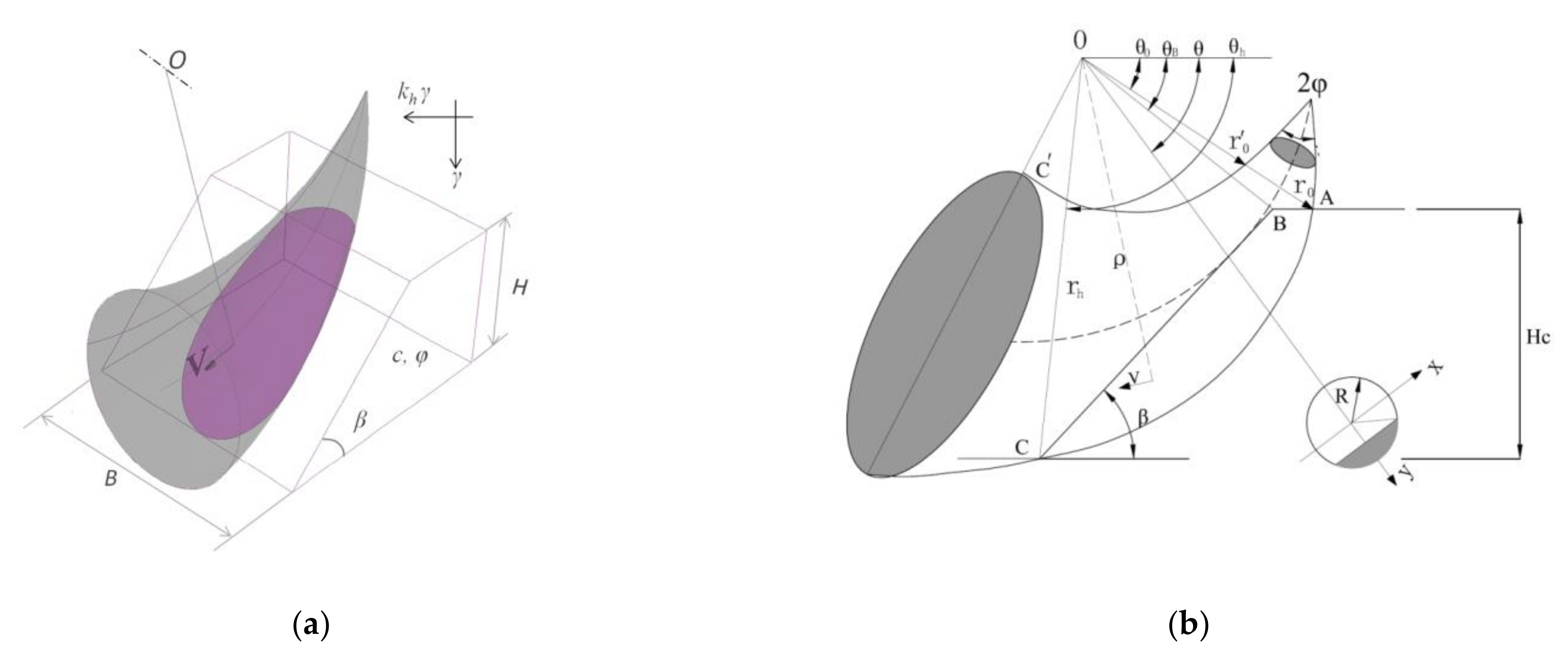
A slope is sketched in Figure 1a, in which β denotes the angle of inclination, H and B represent the slope height and width, respectively, and c and φ are the soil cohesion and friction angle, respectively. The slope was subjected to two external forces, gravity and the earthquake loadings. The pseudo-static approach was employed herein to consider the seismic effect, which was assumed to be uniform inertial forces and equal to the soil unit weight (γ) multiplied by a so-called seismic acceleration coefficient (kh). Under the contributions of these two external forces, the slope was about to fail. In order to check the three-dimensional stability of slopes, the three-dimensional (3D) rotational horn-type mechanism, proposed by Michalowski and Drescher [22], was employed in this study, combining the pseudo-static method with the upper-bound limit analysis. The 3D horn-type failure mechanism of slopes is sketched in Figure 1b. The horn-type failure mechanism is composed of the 3D horn section split by a plane-strain insert body. In the longitudinal symmetry plane, the contours of the horn-type failure mechanism are described by two log-spirals. The 3D horn section, crossing the slope toe, partly intersects the slope body, which defines the moving part of the slope at failure. The plane-strain insert section with width b was inserted into the horn section to make the analysis reduce to two-dimensional analysis results when the slope width was not confined. The whole composite failure mechanism followed a rotational velocity field with respect to the center O. The cross section of the 3D horn body had to be a circle in order to meet the kinematic admissibility required by the norm rule based on the limit analysis method [22]. The 3D horn-type failure mechanism was completely determined by four geometrical parameters.
In order to derive the critical slope height based on the upper-bound limit analysis [22], both the external work rate and the internal energy dissipation had to be calculated in terms of the assumed 3D horn-type failure mechanism. In this study, the external force mainly referred to the earthquake shaking forces and the gravity, while the internal energy dissipation included those in the volume and along the failure surface. The external work rate of gravity and internal energy dissipation could be directly obtained from [22]. The pseudo-static method was used herein to represent the earthquake shaking forces to compute its external work rate, in which the horizontal seismic coefficient was a necessary and important input parameter. Thus, an assessment of the critical slope height with the 3D horn-type failure mechanism can be written as
The expression of can be found in the Appendix A. The critical slope height was searched by optimization using the genetic algorithm with respect to the four geometrical parameters.
4. Input Random Variables
According to Equations (5) and (6), six input parameters are essential to compute the safety factor of slopes in this study, including the soil Mohr–Coulomb shear strength parameters (soil cohesion c and friction angle φ), the horizontal seismic acceleration coefficient (kh), the slope geometrical parameters (slope inclination β, width H, and width–height ratio B/H). and the unit weight of soil masses (γ). In order to examine the influence of uncertainties in these model parameters, they were considered as random variables. Their statistical properties are given in Table 1. The Latin hypercube sampling technique was used to generate samples according to their distributions. The benefit of LHS is that it generates samples that distribute as evenly as possible over the sampling space.
In Table 1, the mean values for soil Mohr–Coulomb shear strength parameters are commonly encountered in geotechnical practice [8]. The degree of uncertainty is described by the coefficients of variation (COVs), and three scenarios in terms of their COVs were considered in this study. According to [8], the value of the COVs of soil friction angle Vφ ranged between 10% and 20%, while the value of the COVs of soil cohesion Vc changed from 10% to 50%. The neutral uncertainty level of the friction angle and the cohesion were set to 10% and 25%, respectively, from which their Pessimistic Scenario and Optimistic Scenario, respectively, were obtained by increasing and reducing by 5%.
The horizontal seismic coefficients, kh, are usually set to a range between 0.0 and 0.3 when the pseudo-static design analysis is used [23]. The statistical properties of the horizontal seismic coefficient reported in the literature are summarized in Table 2 [10,11,12,13]. Other input parameters, including the slope angle β, the width–height ratio B/H, and the unit weight of soil masses γ, were also considered as random variables, as seen in Table 1, with a low randomness compared with the shear strength parameters and the horizontal seismic coefficient.
5. Results and Discussions
The influence of the uncertainty degree, correlation structures, and distribution types of the six input random variables on the assessed probabilistic density functions, failure probability, and sensitivity analysis using the method of SPCE-MCS were investigated and discussed in this section.
5.1. Influence of Uncertainty Degrees
The impact of uncertainty degrees on the probabilistic analysis results, including probability density functions (PDFs) of the critical slope heights (Hc), sensitivity analysis, and failure probability, were studied. It was assumed that the six input variables followed lognormal distributions.
5.1.1. Influence on PDFs
The effects of the three uncertainty scenarios on the probability density functions of the critical slope height are given in Figure 2. The critical slope heights were normalized by the mean value of the cohesion and the unit weight of soil masses in this plot. As shown in Figure 2, the shape of PDFs was largely affected by the uncertainty levels. A higher uncertainty level leads to a shorter and wider shape of PDFs. This was expected, since lower COVs of input parameters should result in higher accuracy, which shows a higher peak in the PDFs. Besides, it could infer that the mean value of the critical slope height was slightly affected by the uncertainty degrees. It was seen that the mean value of the normalized slope critical height decreased slightly with the changing of the uncertainty degrees of the input parameters.
5.1.2. Influence on Computed Failure Probabilities
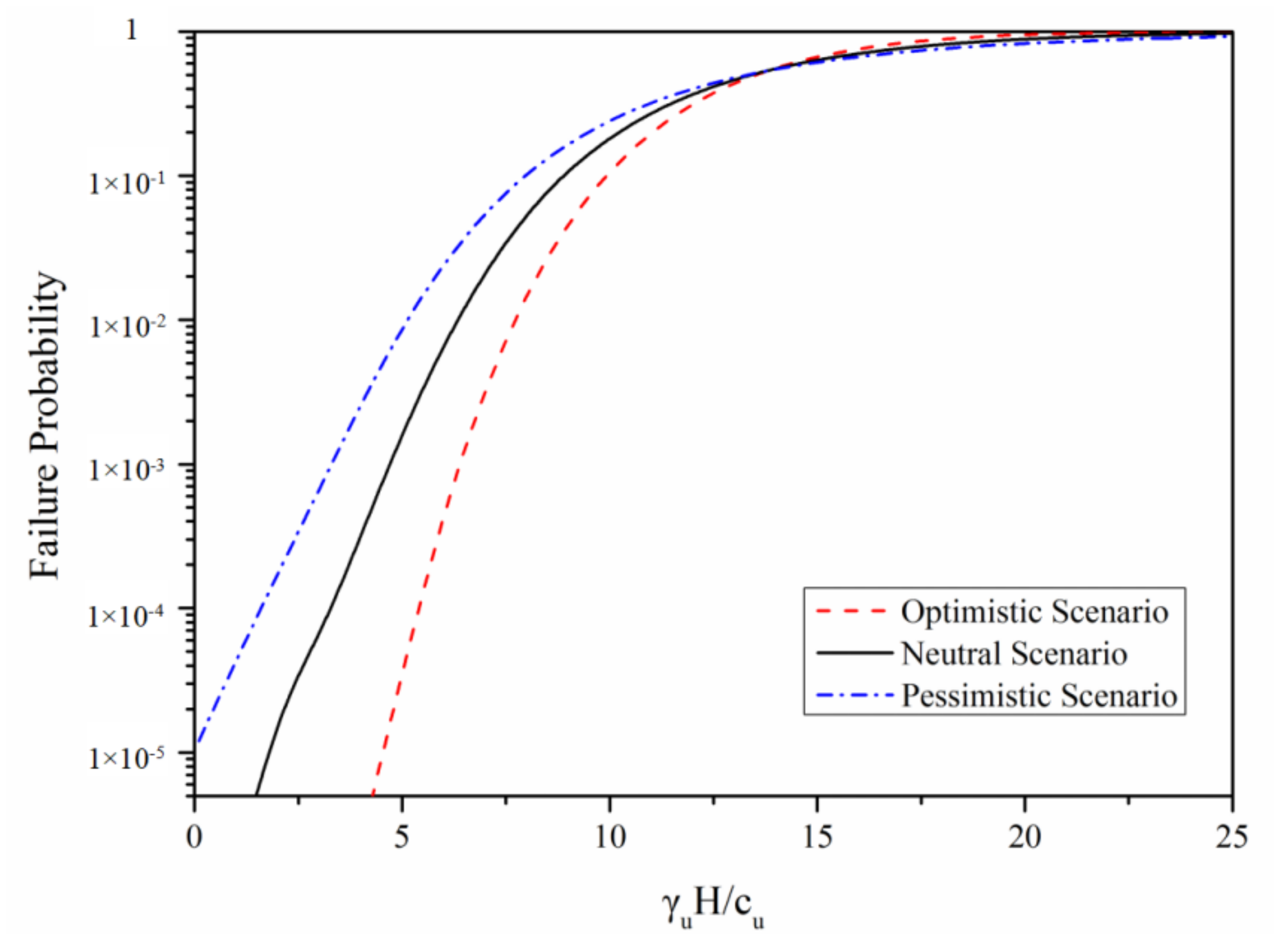
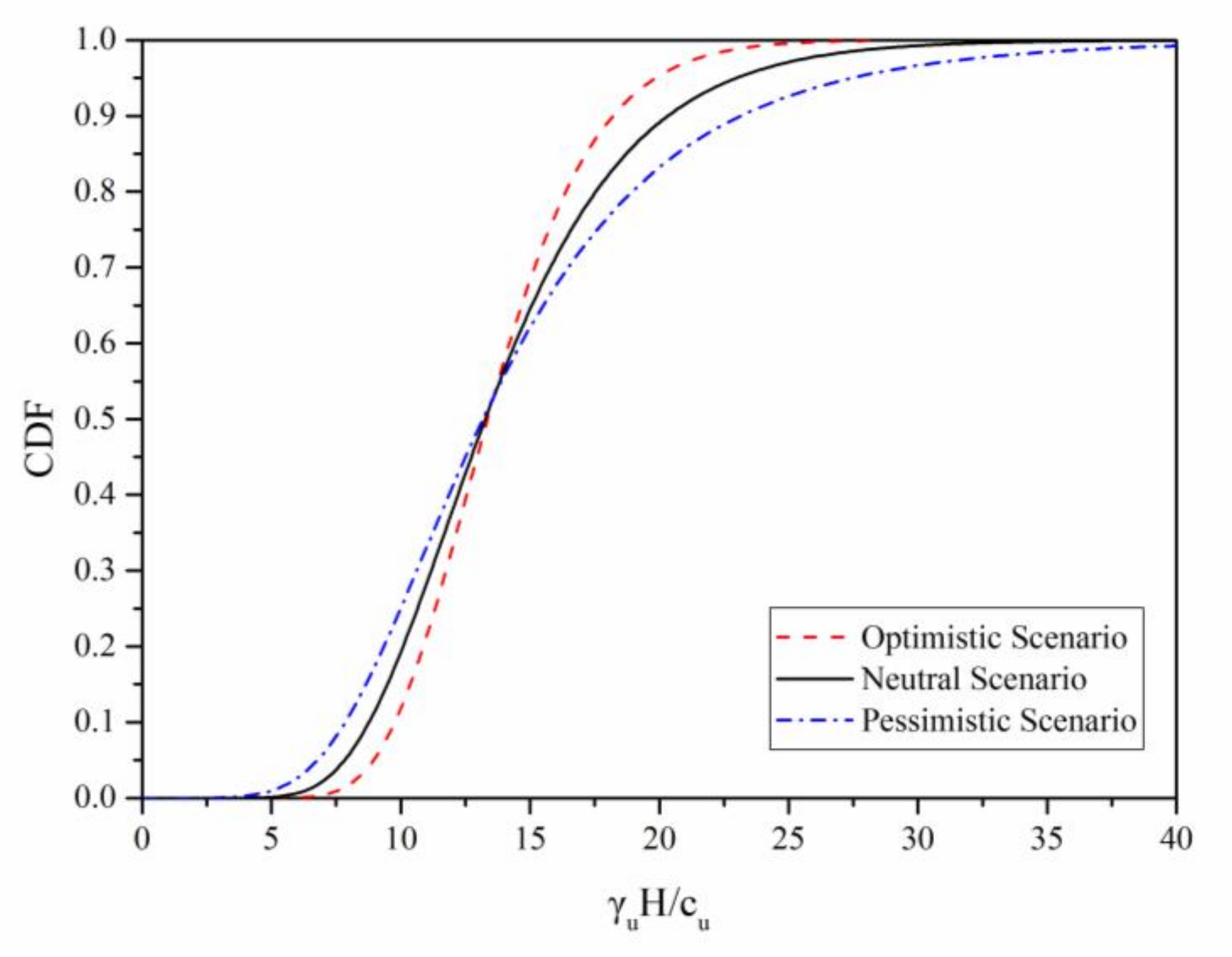
The computed failure probabilities under different uncertainty levels versus the normalized critical slope height are plotted in Figure 3. The coefficient of variation of slope height was also taken into account in this analysis. It can be seen from Figure 3 that the computed failure probabilities largely increased as the critical slope height became large. It is also known that a higher uncertainty level results in a higher failure probability when the normalized critical slope height γuH/c < 14. For instance, in the case of γuH/c = 10, the failure probability increased from 11.7% to 25.1% when the uncertainty level changed from the Optimistic Scenario to the Pessimistic Scenario. On the contrary, when γuH/c > 14, the opposite trends manifested as the increase of uncertainty level, with a higher uncertainty tending to result in lower failure probabilities. The corresponding curves of cumulative distribution functions (CDFs) are shown in Figure 4, which can explain this special phenomenon. The Optimistic uncertainty levels, i.e., the greatest values of COVs in input variables, provided the highest computed failure probabilities after γuH/c exceeded 14.
5.1.3. Influence on Sobol’ Index
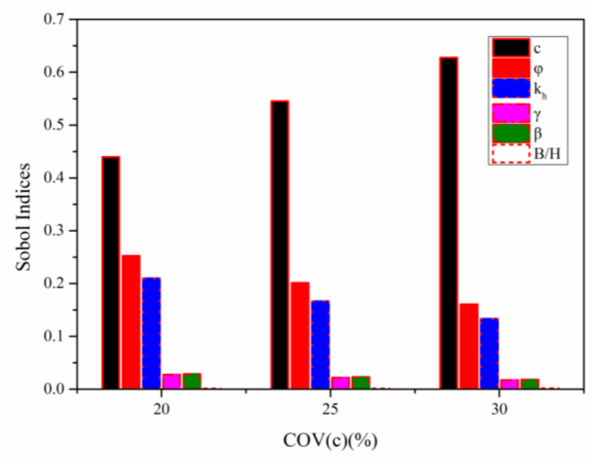
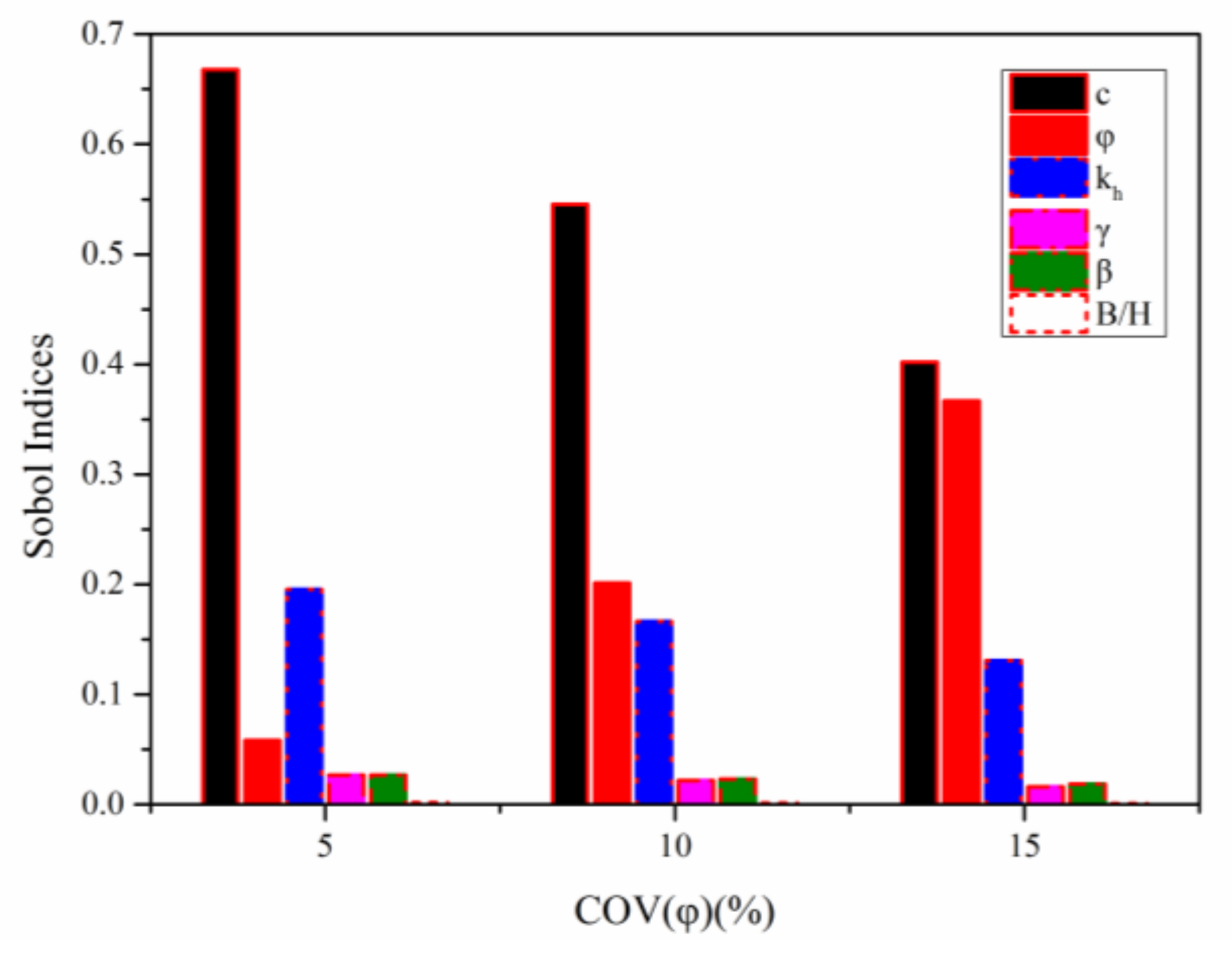
To investigate the impact of the uncertainty degrees of the soil shear parameters on the global sensitivity analysis, three COV scenarios of the friction angle and the cohesion were considered in this section, while four other parameters were fixed at the Neutral Scenario. Figure 5 and Figure 6, respectively, plot the influence of the uncertainty degrees of the cohesion c and the friction angle φ on the results of Sobol’ indices. In this study, only the Sobol’ indices of an individual input parameter were presented in Figure 5 and Figure 6.
It can be seen that the variation of COV of the shear strength parameters greatly affects the Sobol’ indices of all input variables. The practical significance of this sensitivity analysis lies in that it can provide guidance for designers to determine the importance of input parameters. Making reference to Figure 5, at COVc = 30%, the Sobol index of the cohesion c was the highest, indicating that c had the largest impact on the critical slope height for this case, followed by the friction angle φ and the horizontal seismic coefficient kh. This means that the friction angle φ and the horizontal seismic coefficient were the second most significant input variables. The Sobol’ indices of the other input parameters in terms of importance were as follows: β > γ > B/H. The ratio B/H was the least important variable, whose Sobol’ indices could be ignored for all cases. It is noted that this ranking in terms of importance is dependent on the coefficient of variation of input parameters. It may change as the level of uncertainty varies. For instance, as shown in Figure 6, the importance of the friction angle φ rose from the third to the second place when the COV varied from 5% to 15%.
5.2. Influence of Correlation Relations
In order to consider the dependence between c and φ, the correlation coefficient rcφ was considered. The values of the correlation coefficient rcφ recommended by several scholars [14,24,25,26,27] are listed in the following Table 3. The value of the correlation coefficient, rcφ = −0.5, was considered in this study. The other parameters were fixed at the Neutral scenario listed in Table 2, and the distribution types of all the input variables were assumed to be lognormal distributions.
5.2.1. Influence on PDFs
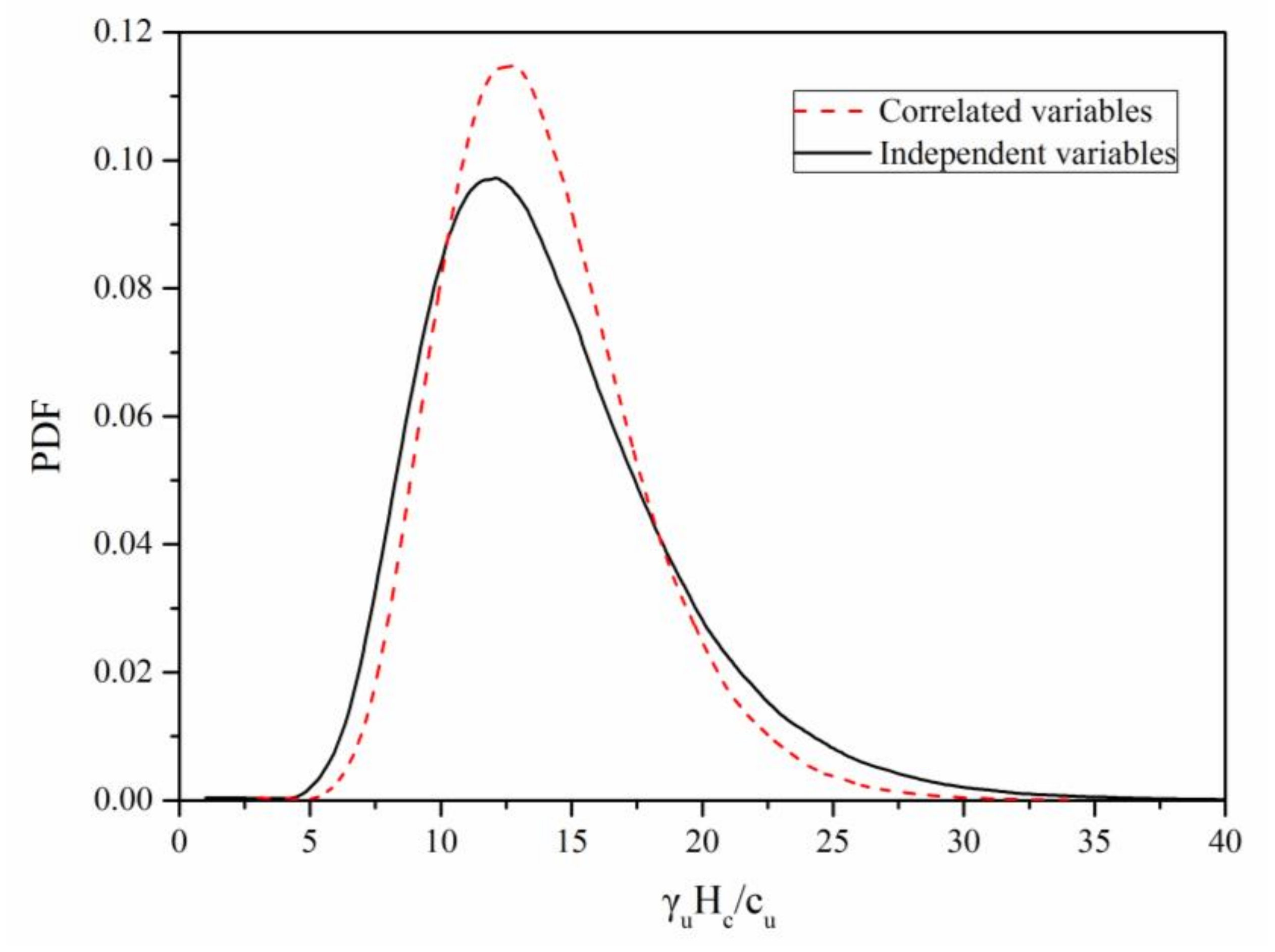
The PDF curves corresponding to correlated and independent shear strength parameters are presented in Figure 7. It can be seen that the correlation between shear strength parameters greatly impacts the shape of PDF curves of the critical slope height. Considering that the correlation between shear strength parameters results in a narrower and higher PDF curve, this indicates that it gives a more robust assessment of the critical slope height Hc when the correlation between shear strength parameters is considered.
5.2.2. Influence on Computed Failure Probabilities
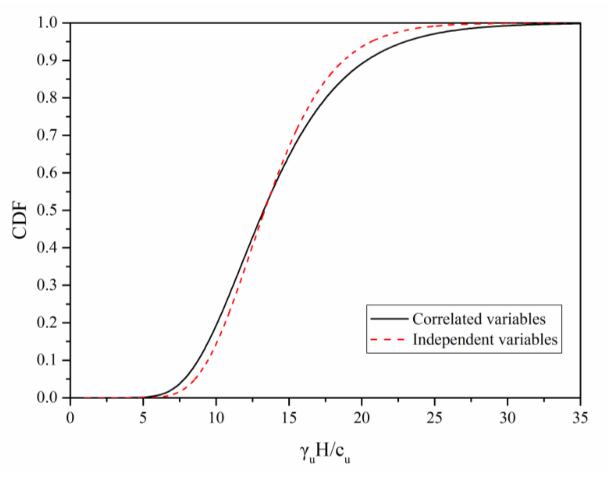
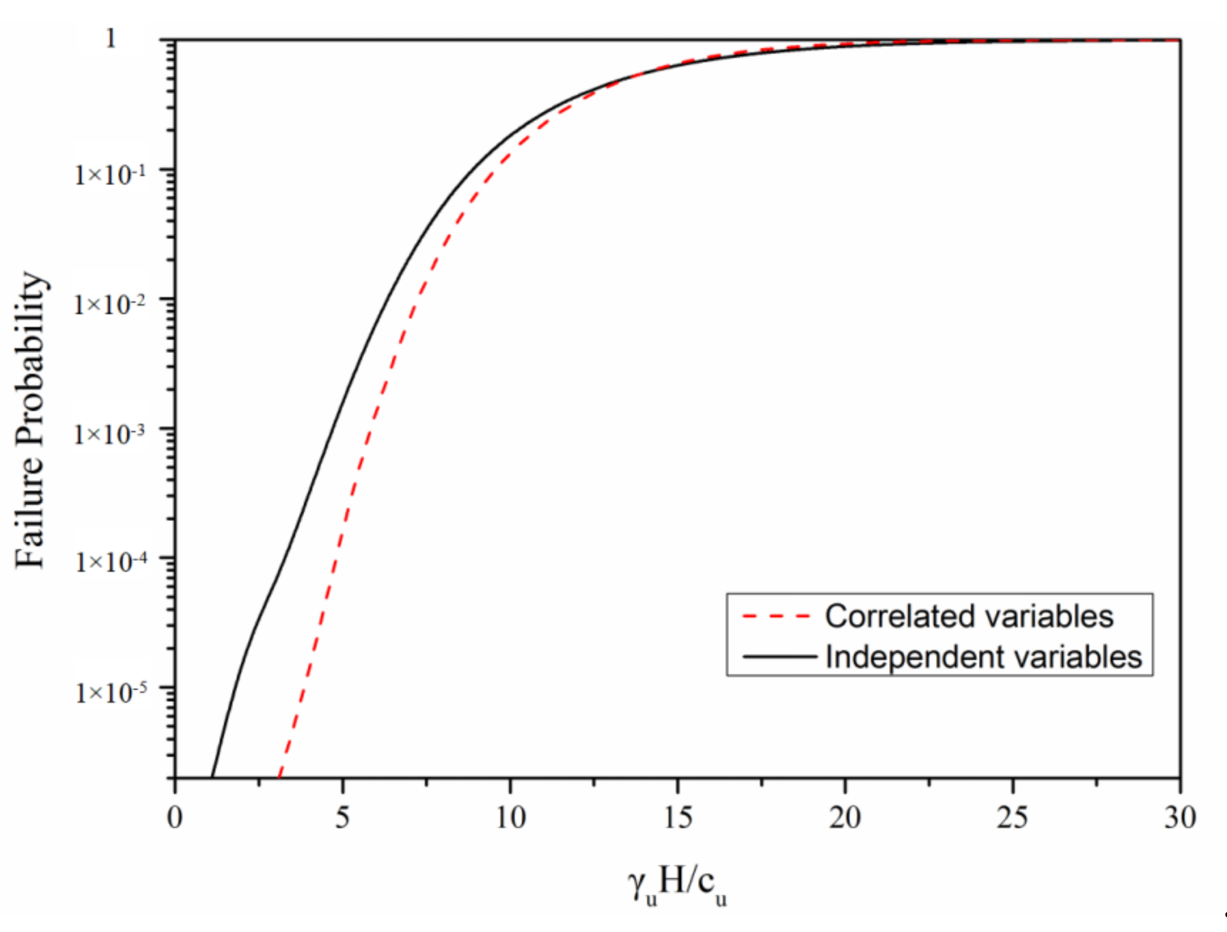
Figure 8 and Figure 9 illustrate the CDF curves and the assessed failure probability for the dependent and independent of shear strength parameters, respectively, versus the normalized critical slope height Hc. As can be seen in Figure 8 and Figure 9, the correlation between shear strength parameters led to a lower failure probability when the normalized critical slope height γuH/c < 14. For example, in the case of γuH/c = 10, the failure probability decreased from 19.3% to 14.4% when the correlation coefficient was taken into account. However, the opposite results were observed when γuH/c > 14. It can be concluded that the impact of considering correlation coefficient is similar to the lower uncertainty level. This makes sense, because a negative correlation between the soil shear strength parameters means that the uncertainty degrees in the calculated shear strength were lower than the combined uncertainty degrees in terms of c and φ when charactering the soil shear strength.
5.3. Influence of Distribution Types
In this section, the impacts of different distribution types on probabilistic density function, failure probability, and sensitivity analysis were investigated. All random variables were assumed to follow lognormal distributions and normal distributions in this section. The input parameters were fixed at the Neutral scenario listed in Table 2.
5.3.1. Influence on PDFs
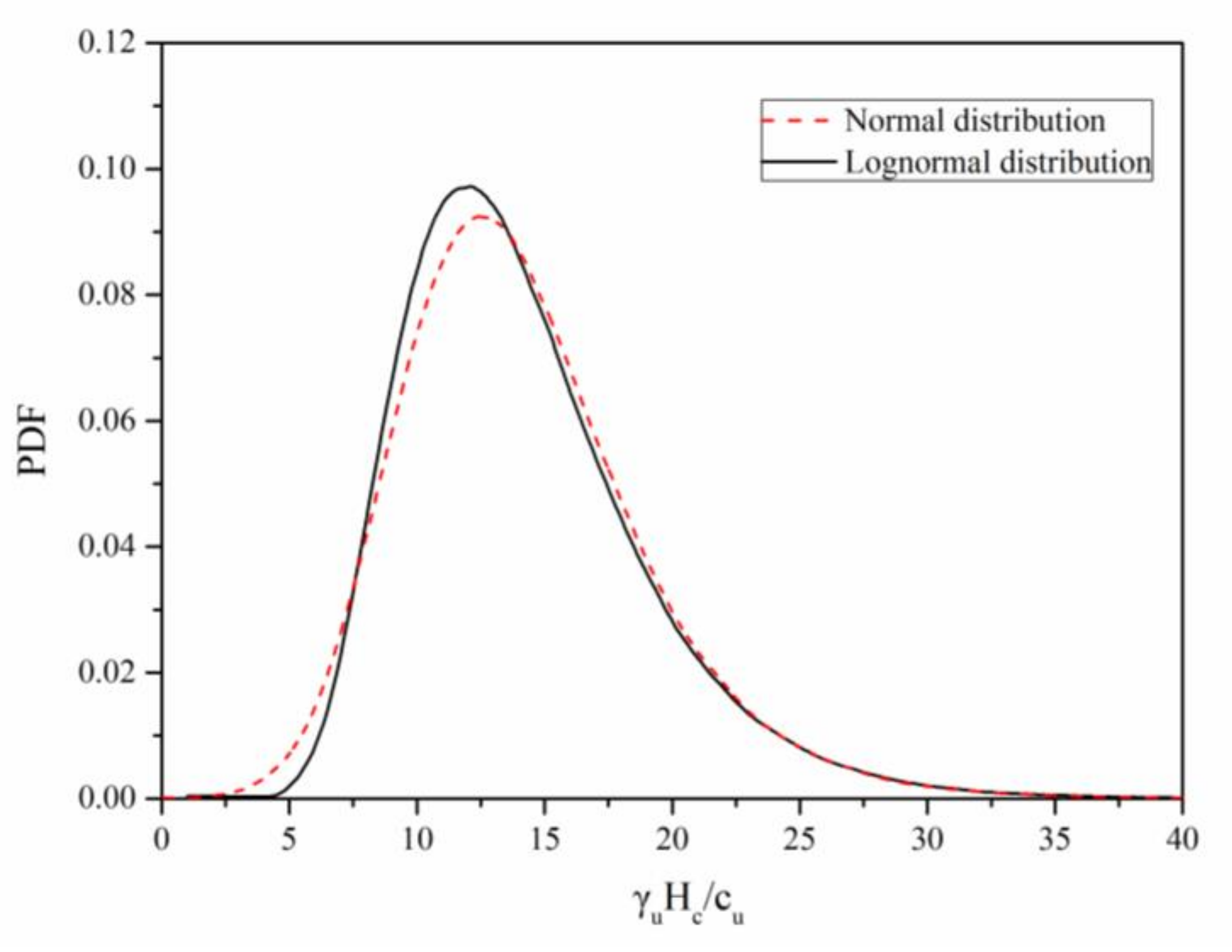
The results of probability density functions of the assessed slope critical heights under lognormal and normal distributions are given in Figure 10. It can be seen in this plot that the normal distribution tended to give a lower and wider curve of PDFs. Besides this, it is interesting that the mean values of critical slope height were almost the same for the two different distributions.
5.3.2. Influence on Computed Failure Probabilities
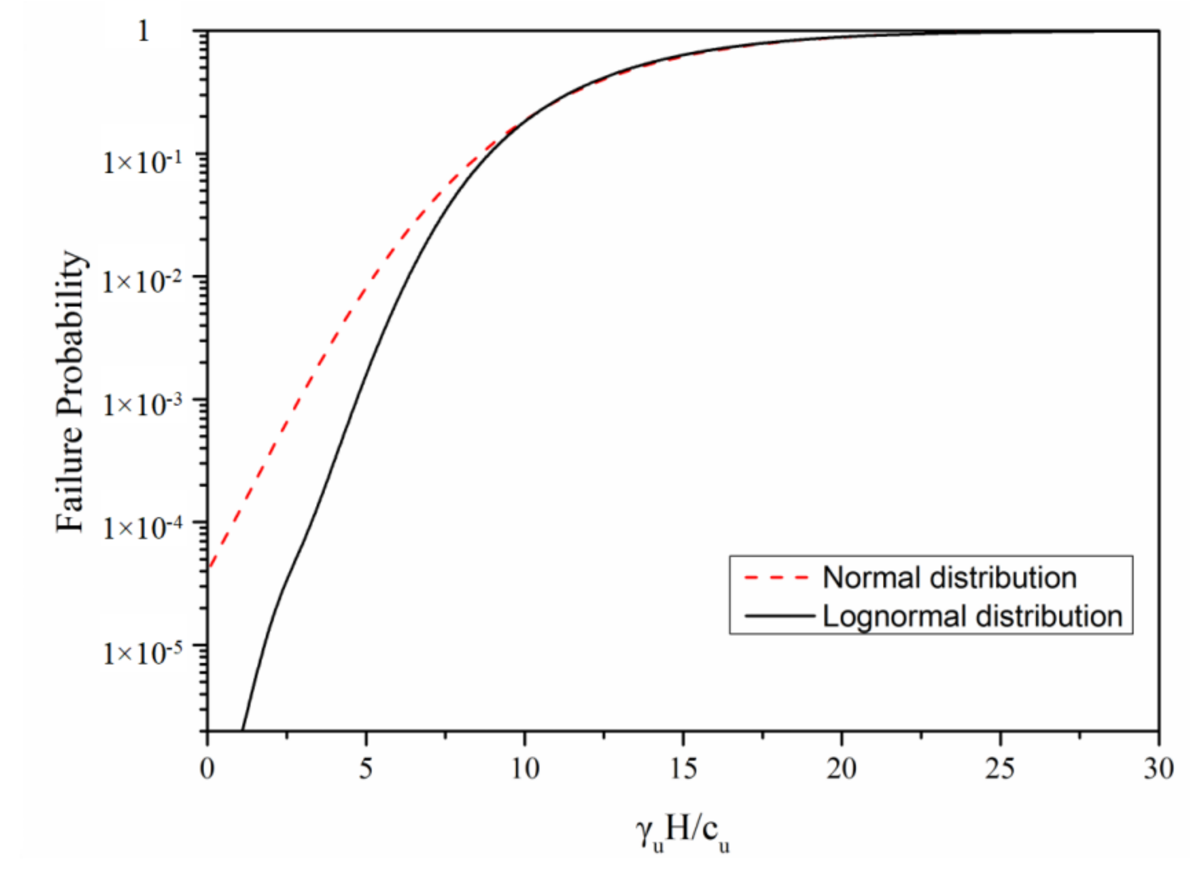
The computed failure probabilities versus the normalized critical slope height Hc were presented in Figure 11 under the case of lognormal and normal distributions. Making reference to Figure 11, compared with the lognormal distribution, the normal distribution led to a higher failure probability, especially when γuH/c < 10. This indicates that the assumption of normal distribution tended to give a conservative result.
5.3.3. Influence on Sobol Index
Sobol’ indices for normal and lognormal distributions are listed in Table 4. It was found that the random variable distributions slightly affect the results of Sobol’ indices. The normal and lognormal distributions provided almost similar results in Sobol’ indices.
6. Conclusions
This paper aimed to study probabilistic stability of soil slopes subject to seismic forces. The method of upper-bound limit analysis combined with the classical pseudo-static analysis was employed to compute the critical slope height by using the three-dimensional rotational horn-type mechanism. This combination is widely accepted in engineering design. The three-dimensional slope probability analysis framework was performed by adopting the method of SPCE-MCS, which led to a more economical estimation of failure probability of a slope. The influences of the variables’ uncertainty degrees, correlation coefficient, and distribution types were investigated particularly.
The uncertainty degrees significantly influenced the results of PDF curves and the assessed failure probabilities. The authors found that the failure probability was dependent not only on the variability of input parameters, but also on slope geometry. It was interesting to see that there exists a critical value of the normalized critical slope height. For example, a higher uncertainty level led to a shorter and wider shape of PDFs and larger failure probabilities at γuH/c < 14, over which a higher variability of model parameters results in a lower failure probability.
The increasing of COV of an individual input parameter resulted in an increase of its Sobol’ index, with simultaneous declining of other input variables. The ranking of the Sobol’ index in terms of importance was dependent on the COV of input parameters, and this may change as the level of uncertainty varies. The horizontal seismic coefficient was the second most important variable compared to the soil shear strength parameters.
The correlation between the soil Mohr–Coulomb shear strength parameters resulted in a narrower and higher PDF curve and led to smaller failure probabilities at γuH/c < 14. The impact of considering the correlation coefficient was similar to the lower uncertainty levels.
The normal distribution tended to give lower and wider curves of PDFs and higher failure probabilities, especially when γuH/c < 10. In the global sensitive analysis, normal distributions and lognormal distributions give almost the same solutions of Sobol indices.
Anthropic activities, such as blasting vibrations, injections, and hydraulic fracturing, would induce ground shaking and pose damage to geotechnical structures. However, the variability of anthropic activities is rather high, resulting from different construction techniques and operating skills. Thus, a topic worthy of a future study is to extend the presented simulations to evaluate the influence of human-induced seismicity on dynamic slope stability analysis in a probabilistic framework.
In this study, the soil masses were considered as homogeneous and isotropic material for simplicity. However, the shear parameters of soils show spatial variability in reality, and it has a significant impact on slope stability, for example, the fluctuation scales. The spatial variability of soil parameters can be well represented by random fields. The influence of fluctuation scales on seismic slope stability will be considered in future studies.
Author Contributions
Writing and Analysis: D.L.; Supervision: M.S.; Resources & Editing: E.Y.; Review & Editing: T.Y. All authors have read and agreed to the published version of the manuscript.
Funding
This research received no external funding.
Institutional Review Board Statement
Not applicable.
Informed Consent Statement
Not applicable.
Data Availability Statement
Not applicable.
Conflicts of Interest
The authors declare no conflict of interest.
Appendix A
References
- Rampello, S.; Callisto, L.; Fargnoli, P. Evaluation of slope performance under earthquake loading conditions. Rivista Italiana di Geotecnica 2010, 44, 29–41. [Google Scholar]
- Aboayanah, K.; Oggeri, C.; Sambuelli, L. A simplified model for injection-induced seismicity: An evaluation of influencing factors. Geoingegneria Ambientale e Mineraria 2019, 158, 45–52. [Google Scholar]
- Deng, D.-P.; Li, L. Limit Equilibrium Analysis of Slope Stability with Coupling Nonlinear Strength Criterion and Double-Strength Reduction Technique. Int. J. Geéoméch. 2019, 19, 04019052. [Google Scholar] [CrossRef]
- Sengani, F.; Mulenga, F. Application of Limit Equilibrium Analysis and Numerical Modeling in a Case of Slope Instability. Sustainability 2020, 12, 8870. [Google Scholar] [CrossRef]
- Michalowski, R.L.; Martel, T. Stability Charts for 3D Failures of Steep Slopes Subjected to Seismic Excitation. J. Geotech. Geoenviron. Eng. 2011, 137, 183–189. [Google Scholar] [CrossRef] [Green Version]
- Pan, Q.; Dias, D. An efficient reliability method combining adaptive Support Vector Machine and Monte Carlo Simulation. Struct. Saf. 2017, 67, 85–95. [Google Scholar] [CrossRef]
- Lancellotta, R. Lower band approach for seismic passive earth resistance. Geotecnique 2007, 57, 319–321. [Google Scholar] [CrossRef]
- Baecher, G.B.; Christian, J.T. Reliability and Statistics in Geotechnical Engineering; John Wiley & Sons: Hoboken, NJ, USA, 2005. [Google Scholar]
- Dodigović, F.; Ivandić, K.; Kovačević, M.S.; Soldo, B. Error Evaluation and Suitability Assessment of Common Reliability Methods in the Case of Shallow Foundations. Appl. Sci. 2021, 11, 795. [Google Scholar] [CrossRef]
- Hynes-Griffin, M.E.; Franklin, A.G. Rationalizing the Seismic Coefficient Method (No. WES/MP/GL-84-13); Army Engineer Waterways Experiment Station Vicksburg Ms Geotechnical Lab: Vicksburg, MS, USA, 1984. [Google Scholar]
- Cao, T.; Petersen, M.D.; Reichle, M.S. Seismic hazard estimate from background seismicity in southern California. Bull. Seismol. Soc. Am. 1996, 86, 1372–1381. [Google Scholar]
- Cramer, C.H. A seismic hazard uncertainty analysis for the New Madrid seismic zone. Eng. Geol. 2001, 62, 251–266. [Google Scholar] [CrossRef]
- Tsompanakis, Y.; Lagaros, N.D.; Psarropoulos, P.N.; Georgopoulos, E.C. Probabilistic seismic slope stability assessment of geostructures. Struct. Infrastruct. Eng. 2010, 6, 179–191. [Google Scholar] [CrossRef]
- Jiang, S.-H.; Li, D.-Q.; Zhang, L.; Zhou, C. Slope reliability analysis considering spatially variable shear strength parameters using a non-intrusive stochastic finite element method. Eng. Geol. 2014, 168, 120–128. [Google Scholar] [CrossRef]
- Guo, X.; Sun, Q.; Dias, D.; Antoinet, E. Probabilistic assessment of an earth dam stability design using the adaptive polynomial chaos expansion. Bull. Int. Assoc. Eng. Geol. 2020, 79, 4639–4655. [Google Scholar] [CrossRef]
- Lins, I.D.; Moura, M.D.C.; Zio, E.; Droguett, E.L. A particle swarm-optimized support vector machine for reliability prediction. Qual. Reliab. Eng. Int. 2012, 28, 141–158. [Google Scholar] [CrossRef]
- Wang, L.; Wu, C.; Gu, X.; Liu, H.; Mei, G.; Zhang, W. Probabilistic stability analysis of earth dam slope under transient seepage using multivariate adaptive regression splines. Bull. Int. Assoc. Eng. Geol. 2020, 79, 2763–2775. [Google Scholar] [CrossRef]
- Wan, H.-P.; Todd, M.D.; Ren, W.-X. Statistical framework for sensitivity analysis of structural dynamic characteristics. J. Eng. Mech. 2017, 143, 04017093. [Google Scholar] [CrossRef]
- Lüthen, N.; Marelli, S.; Sudret, B. Sparse Polynomial Chaos Expansions: Literature Survey and Benchmark. SIAM/ASA J. Uncertain. Quantif. 2021, 9, 593–649. [Google Scholar] [CrossRef]
- Shao, Q.; Younes, A.; Fahs, M.; Mara, T. Bayesian sparse polynomial chaos expansion for global sensitivity analysis. Comput. Methods Appl. Mech. Eng. 2017, 318, 474–496. [Google Scholar] [CrossRef] [Green Version]
- Blatman, G.; Sudret, B. Adaptive sparse polynomial chaos expansion based on least angle regression. J. Comput. Phys. 2011, 230, 2345–2367. [Google Scholar] [CrossRef]
- Michalowski, R.; Drescher, A. Three-dimensional stability of slopes and excavations. Géotechnique 2009, 59, 839–850. [Google Scholar] [CrossRef]
- Baker, R.; Shukha, R.; Operstein, V.; Frydman, S. Stability charts for pseudo-static slope stability analysis. Soil Dyn. Earthq. Eng. 2006, 26, 813–823. [Google Scholar] [CrossRef]
- Wolff, T. Analysis and Design of Embankment Dam Slopes: A Probabilistic Approach (Soil Mechanics, Indiana). Ph.D. Thesis, Purdue University, Lafayette, IN, USA, 1986. [Google Scholar]
- Yucemen, M.S.; Tang, W.H.; Ang, A.S. A Probabilistic Study of Safety and Design of Earth Slopes; University of Illinois Engineering Experiment Station. College of Engineering. University of Illinois at Urbana-Champaign: Urbana, IL, USA, 1973. [Google Scholar]
- Lumb, P. Safety factors and the probability distribution of soil strength. Can. Geotech. J. 1970, 7, 225–242. [Google Scholar] [CrossRef]
- Cho, S.E. Probabilistic Assessment of Slope Stability That Considers the Spatial Variability of Soil Properties. J. Geotech. Geoenviron. Eng. 2010, 136, 975–984. [Google Scholar] [CrossRef]
Figure 1.
Sketch of (a) the slope problem under study and (b) the associated 3D rotational failure mechanism.
Figure 1.
Sketch of (a) the slope problem under study and (b) the associated 3D rotational failure mechanism.

Figure 2.
Impact of uncertainty level on PDF with the critical slope height normalized by the soil unit weight and cohesion.
Figure 2.
Impact of uncertainty level on PDF with the critical slope height normalized by the soil unit weight and cohesion.

Figure 3.
Failure probability under three uncertainty levels as a function of the critical slope height normalized by the soil unit weight and cohesion.
Figure 3.
Failure probability under three uncertainty levels as a function of the critical slope height normalized by the soil unit weight and cohesion.

Figure 4.
Curves of CDF under three probabilistic scenario with the critical slope height normalized by the soil unit weight and cohesion.
Figure 4.
Curves of CDF under three probabilistic scenario with the critical slope height normalized by the soil unit weight and cohesion.

Figure 5.
Impact of COVs on Sobol’ Index for cohesion c.

Figure 6.
Impact of COVs on Sobol’ Index for friction angle φ.

Figure 7.
Impact of correlation on PDF with the critical slope height normalized by the soil unit weight and cohesion.
Figure 7.
Impact of correlation on PDF with the critical slope height normalized by the soil unit weight and cohesion.

Figure 8.
Impact of correlations on CDF with the critical slope height normalized by the soil unit weight and cohesion.
Figure 8.
Impact of correlations on CDF with the critical slope height normalized by the soil unit weight and cohesion.

Figure 9.
Impact of correlation on failure probability as a function of the critical slope height normalized by the soil unit weight and cohesion.
Figure 9.
Impact of correlation on failure probability as a function of the critical slope height normalized by the soil unit weight and cohesion.

Figure 10.
Impact of distribution types on PDF.

Figure 11.
Impact of distribution types on failure probability.


Table 1.
Statistics for Input Random Variables.
| Input Variable | Mean(μ) | COV (%) | Distribution Type | ||
|---|---|---|---|---|---|
| Optimistic Scenario | Neutral Scenario | Pessimistic Scenario | |||
| φ (°) | 30.0 | 5.0 | 10.0 | 15.0 | Normal/lognormal |
| c (kPa) | 20.0 | 20.0 | 25.0 | 30.0 | Normal/lognormal |
| kh | 0.2 | 20 | 25.0 | 30 | Normal/lognormal |
| γ (kN/m3) | 20.0 | 3 | 5 | 8 | Normal/lognormal |
| β (°) | 50 | 1.0 | 3.0 | 5.0 | Normal/lognormal |
| B/H | 5.0 | 1.0 | 2.5 | 4.0 | Normal/lognormal |
Table 2.
Statistical Properties for input variable kh.
| Range | Mean(μ) | COV (%) | Distribution Type | Ref. |
|---|---|---|---|---|
| 0.01–0.5 | 0.2 | 10 | lognormal | Tsompanakis et al., 2010 |
| 0.0–0.3 | 0.15 | / | / | Hynes-Griffin and Franklin 1984 |
| 0.0–0.77 | 0.69 | 42 | / | Cramer, 2001 |
| / | / | 10–30 | / | Cao et al., 1996 |
Table 3.
Summary of correlation coefficients between c and φ.
| Recommended Values | Ref. |
|---|---|
| 0.25 (CU), −0.47 (CD) | Wolff, 1985 |
| −0.49 to −0.24 | Yucemen et al., 1973 |
| −0.7 to −0.37 | Lumb, 1970 |
| −0.5 | Cho, 2010 |
| −0.7 | Jiang et al., 2014 |
Note: CU representing consolidated–undrained tests, CD representing consolidated–drained tests.
Table 4.
Results of Sobol’ indices.
| Sobol’ Index | Normal Distribution | Lognormal Distribution |
|---|---|---|
| c | 0.5275 | 0.5455 |
| φ | 0.1939 | 0.2011 |
| kh | 0.1875 | 0.1663 |
| γ | 0.0214 | 0.0218 |
| β | 0.0225 | 0.0229 |
| B/H | 0.0011 | 0.0014 |
Publisher’s Note: MDPI stays neutral with regard to jurisdictional claims in published maps and institutional affiliations. |
© 2021 by the authors. Licensee MDPI, Basel, Switzerland. This article is an open access article distributed under the terms and conditions of the Creative Commons Attribution (CC BY) license (https://creativecommons.org/licenses/by/4.0/).
Share and Cite
MDPI and ACS Style
Li, D.; Sun, M.; Yan, E.; Yang, T. The Effects of Seismic Coefficient Uncertainty on Pseudo-Static Slope Stability: A Probabilistic Sensitivity Analysis. Sustainability 2021, 13, 8647. https://0-doi-org.brum.beds.ac.uk/10.3390/su13158647
AMA Style
Li D, Sun M, Yan E, Yang T. The Effects of Seismic Coefficient Uncertainty on Pseudo-Static Slope Stability: A Probabilistic Sensitivity Analysis. Sustainability. 2021; 13(15):8647. https://0-doi-org.brum.beds.ac.uk/10.3390/su13158647
Chicago/Turabian StyleLi, Dongli, Miaojun Sun, Echuan Yan, and Tao Yang. 2021. "The Effects of Seismic Coefficient Uncertainty on Pseudo-Static Slope Stability: A Probabilistic Sensitivity Analysis" Sustainability 13, no. 15: 8647. https://0-doi-org.brum.beds.ac.uk/10.3390/su13158647
Note that from the first issue of 2016, this journal uses article numbers instead of page numbers. See further details here.