
Multi-Objective Particle Swarm Optimization-Based Decision Support Model for Integrating Renewable Energy Systems in a Korean Campus Building


Abstract
:1. Introduction
2. Research Methodology
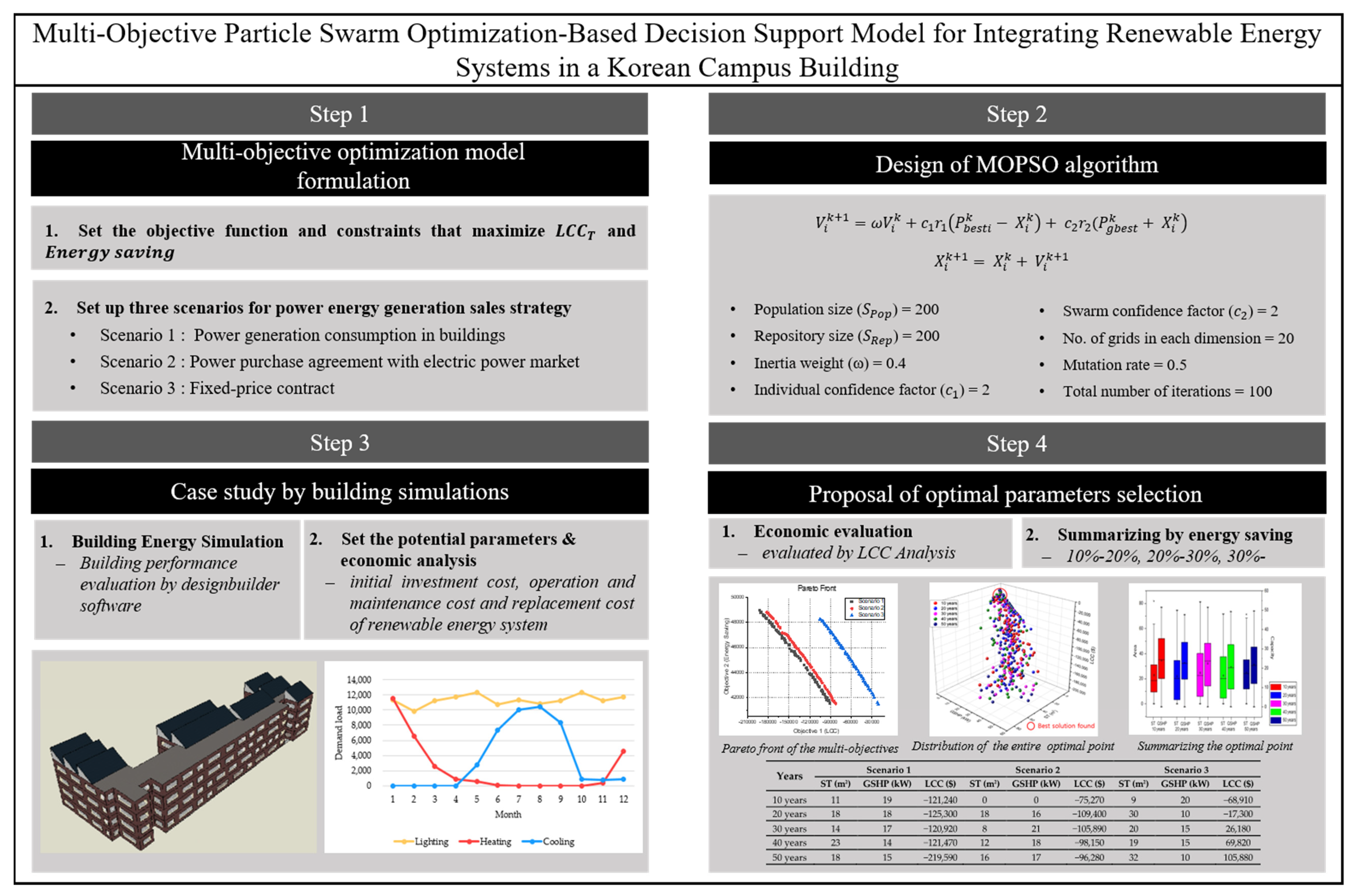
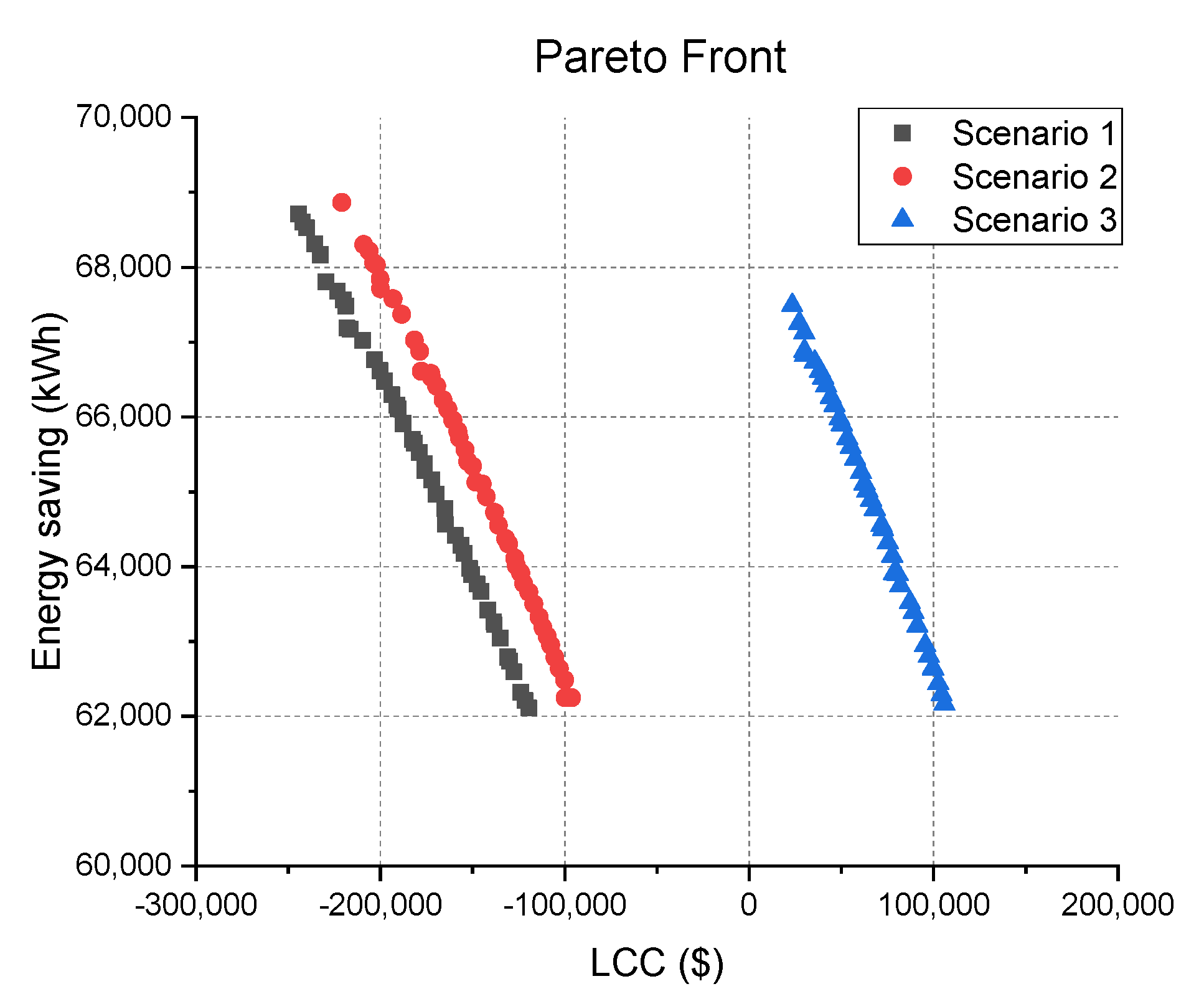
2.1. Power Generation Sales Strategy
- Scenario 1: Power generation consumption in buildings.
- Scenario 2: PPA with electric power market.
- Scenario 3: Fixed-price contract.
2.2. MOPSO Algorithm
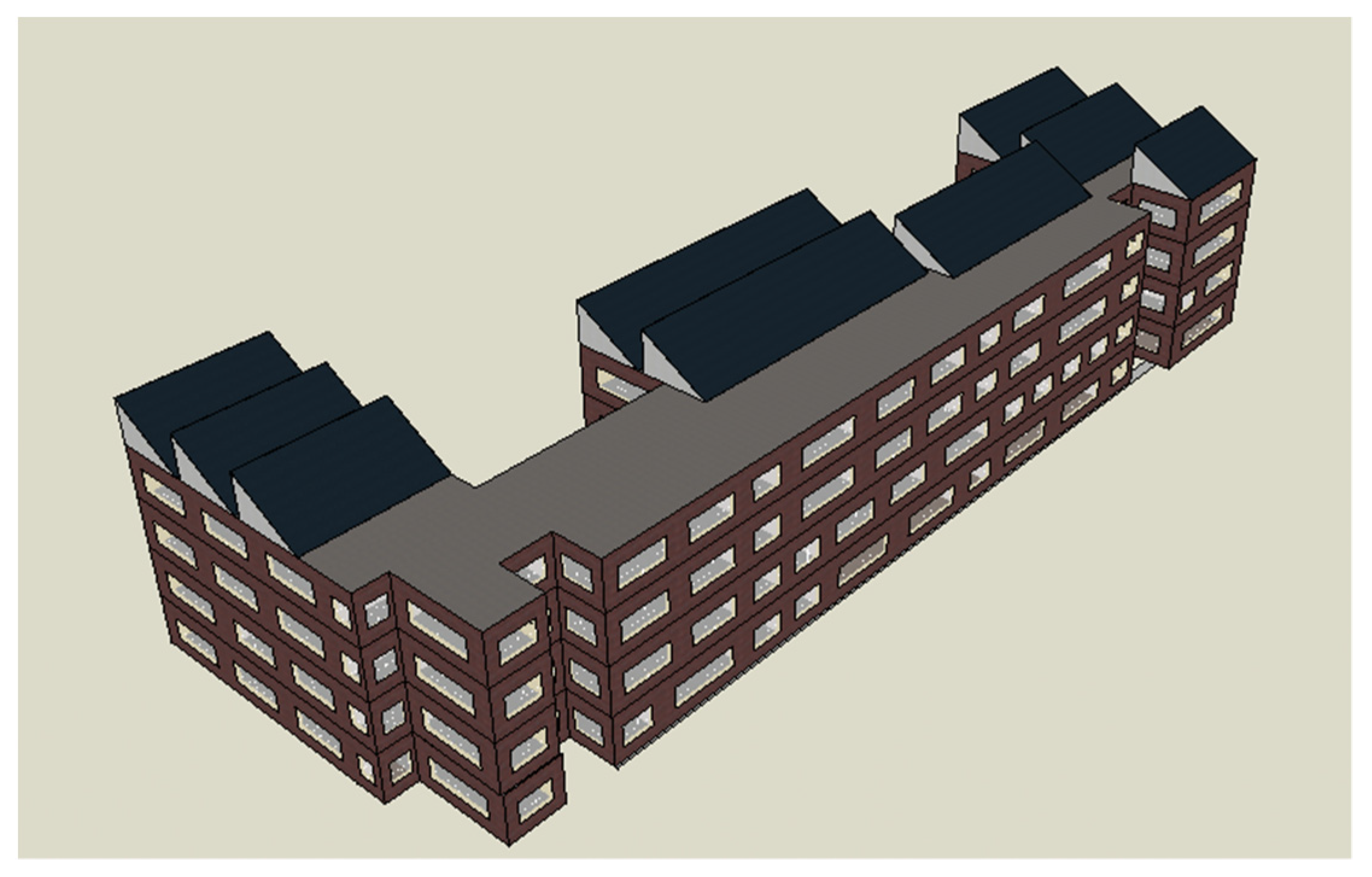
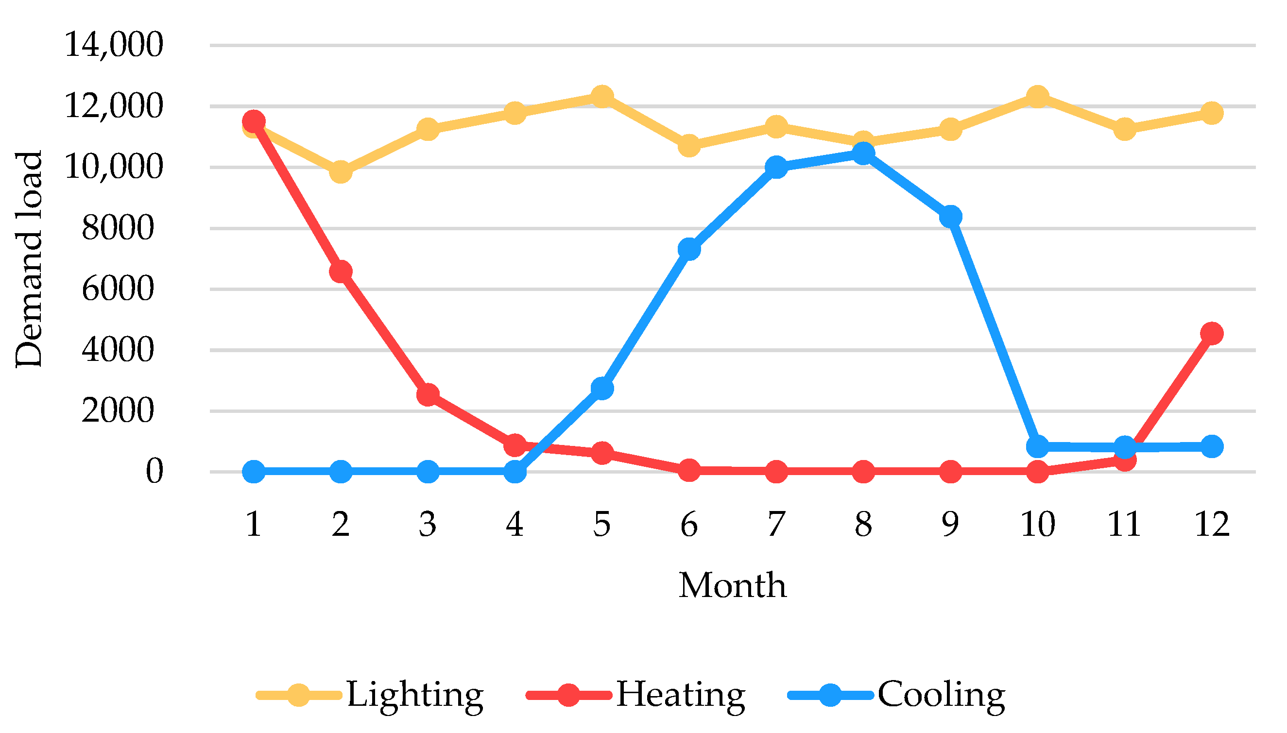
3. Case Study
4. Results and Discussion
5. Conclusions
Author Contributions
Funding
Conflicts of Interest
Nomenclature
| Total amount used for the entire project period | |
| Operation and maintenance cost | |
| Sum of PV NPV | |
| Initial investment cost | |
| Sum of GSHP NPV | |
| Replacement cost | |
| Sum of ST NPV | |
| Real discount rate | |
| Electricity price | |
| Inflation rate | |
| Monetary benefit from the energy generation | |
| Energy unit price for each scenario | |
| Power generation of PV | |
| Power generation of GSHP | |
| Power generation of ST | |
| Objective energy saving | |
| Net area of PV panel surface | |
| Total solar radiation incident on PV array | |
| Fraction of surface area with active solar cells | |
| Direct current to alternating current conversion efficiency | |
| Module conversion efficiency | |
| Empirically determined correction factor | |
| Total solar radiation on solar heat collectors | |
| Product of all transmittance and absorptance terms | |
| Overall heat loss coefficient combining radiation, conversion and conduction terms | |
| Inlet temperature of the working fluid | |
| Outdoor air temperature | |
| Equation fit coefficients | |
| Volumetric flow rate of the load side | |
| Volumetric flow rate of the source side | |
| Volumetric flow rate of the reference load side | |
| Volumetric flow rate of the reference source side | |
| Load side entering water temperature | |
| Source side entering water temperature | |
| Reference temperature |
References
- Waide, P.; Gerundino, D. International standards to develop and promote energy efficiency and renewable energy sources. IEA Inf. Pap. Retrieved 2007, 6, 2011. [Google Scholar]
- Harish, V.S.K.V.; Kumar, A. A review on modeling and simulation of building energy systems. Renew. Sustain. Energy Rev. 2016, 56, 1272–1292. [Google Scholar] [CrossRef]
- Chung, M.H.; Rhee, E.K. Potential opportunities for energy conservation in existing buildings on university campus: A field survey in Korea. Energy Build. 2014, 78, 176–182. [Google Scholar] [CrossRef]
- Del Granado, P.C.; Wallace, S.W.; Pang, Z. The value of electricity storage in domestic homes: A smart grid perspective. Energy Syst. 2014, 5, 211–232. [Google Scholar] [CrossRef]
- Zhang, K.; Li, J.; He, Z.; Yan, W. Microgrid energy dispatching for industrial zones with renewable generations and electric vehicles via stochastic optimization and learning. Phys. A Stat. Mech. Appl. 2018, 501, 356–369. [Google Scholar] [CrossRef]
- Del Granado, P.C.; Pang, Z.; Wallace, S.W. Synergy of smart grids and hybrid distributed generation on the value of energy storage. Appl. Energy 2016, 170, 476–488. [Google Scholar] [CrossRef] [Green Version]
- Iris, Ç.; Lam, J.S.L. A review of energy efficiency in ports: Operational strategies, technologies and energy management systems. Renew. Sustain. Energy Rev. 2019, 112, 170–182. [Google Scholar] [CrossRef]
- Iris, Ç.; Lam, J.S.L. Optimal energy management and operations planning in seaports with smart grid while harnessing renewable energy under uncertainty. Omega (UK) 2021, 103, 102445. [Google Scholar] [CrossRef]
- Kalogirou, S.A. Building integration of solar renewable energy systems towards zero or nearly zero energy buildings. Int. J. Low-Carbon Technol. 2015, 10, 379–385. [Google Scholar] [CrossRef] [Green Version]
- Ahmadi, M.H.; Seyyedsadaghiani, M.; Ghazvini, M.; Shahriar, S.; Nazari, M.A. Ground source heat pump carbon emissions and ground-source heat pump systems for heating and cooling of buildings: A review. Environ. Prog. Sustain. Energy 2018, 37, 1241–1265. [Google Scholar] [CrossRef]
- Beckers, B. Solar Energy at Urban Scale; John Wiley & Sons: Hoboken, NJ, USA, 2012. [Google Scholar]
- Korea Power Exchange. Electric Power Statistics Information System (EPSIS); Korea Power Exchange: Naju-si, Korea, 2017. [Google Scholar]
- Kumbaroğlu, G.; Madlener, R. Evaluation of economically optimal retrofit investment options for energy savings in buildings. Energy Build. 2012, 49, 327–334. [Google Scholar] [CrossRef]
- Hong, T.; Kim, J.; Lee, M. A multi-objective optimization model for determining the building design and occupant behaviors based on energy, economic, and environmental performance. Energy 2019, 174, 823–834. [Google Scholar] [CrossRef]
- Fesanghary, M.; Asadi, S.; Geem, Z.W. Design of low-emission and energy-efficient residential buildings using a multi-objective optimization algorithm. Build. Environ. 2012, 49, 245–250. [Google Scholar] [CrossRef]
- Diakaki, C.; Grigoroudis, E.; Kabelis, N.; Kolokotsa, D.; Kalaitzakis, K.; Stavrakakis, G. A multi-objective decision model for the improvement of energy efficiency in buildings. Energy 2010, 35, 5483–5496. [Google Scholar] [CrossRef]
- Elbaset, A.A.; Barakat, S.; Ibrahim, H. Multi-objective optimization of grid-connected pv-wind hybrid system considering reliability, cost, and environmental aspects. Sustain. Cities Soc. 2020, 60, 102178. [Google Scholar]
- Asadi, E.; da Silva, M.G.; Antunes, C.H.; Dias, L. A multi-objective optimization model for building retrofit strategies using TRNSYS simulations, GenOpt and MATLAB. Build. Environ. 2012, 56, 370–378. [Google Scholar] [CrossRef]
- Wright, J.A.; Loosemore, H.A.; Farmani, R. Optimization of building thermal design and control by multi-criterion genetic algorithm. Energy Build. 2002, 34, 959–972. [Google Scholar] [CrossRef]
- Malatji, E.M.; Zhang, J.; Xia, X. A multiple objective optimisation model for building energy efficiency investment decision. Energy Build. 2013, 61, 81–87. [Google Scholar] [CrossRef] [Green Version]
- Mercado, K.D.; Jimenez, J.; Quintero, M.C.G. Hybrid renewable energy system based on intelligent optimization techniques. In Proceedings of the 2016 IEEE International Conference on Renewable Energy Research and Applications (ICRERA), Birmingham, UK, 20–23 November 2016; pp. 1–6. [Google Scholar]
- González, A.; Riba, J.R.; Rius, A.; Puig, R. Optimal sizing of a hybrid grid-connected photovoltaic and wind power system. Appl. Energy 2015, 154, 752–762. [Google Scholar] [CrossRef] [Green Version]
- Donald, R.; Nieto, A. A Compendium and comparison of 25 project evaluation techniques. Part 1: Net present value and rate of return methods. Int. J. Prod. Econ. 1995, 42, 79–96. [Google Scholar]
- Koo, C.; Hong, T.; Kim, J.; Kim, H. An integrated multi-objective optimization model for establishing the low-carbon scenario 2020 to achieve the national carbon emissions reduction target for residential buildings. Renew. Sustain. Energy Rev. 2015, 49, 410–425. [Google Scholar] [CrossRef]
- Bae, S.; Nam, Y.; da Cunha, I. Economic solution of the tri-generation system using photovoltaic-thermal and ground source heat pump for zero energy building (ZEB) realization. Energies 2019, 12, 3304. [Google Scholar] [CrossRef] [Green Version]
- Suh, H.S.; Kim, D.D. Energy performance assessment towards nearly zero energy community buildings in South Korea. Sustain. Cities Soc. 2019, 44, 488–498. [Google Scholar] [CrossRef]
- Korea energy Agency. Renewable Energy Supply Status; Korea Energy Agency: Ulsan, Korea, 2018. [Google Scholar]
- Gul, M.; Kotak, Y.; Muneer, T. Review on recent trend of solar photovoltaic technology. Energy Explor. Exploit. 2016, 34, 485–526. [Google Scholar] [CrossRef] [Green Version]
- Clerc, M. Particle Swarm Optimization; John Wiley & Sons: Hoboken, NJ, USA, 2010; pp. 1942–1948. [Google Scholar]
- Moon, J.; Yoon, Y.; Kim, S.; Kim, K.; Kim, S.; Kim, J. Virtual optimal design of satellite adapter in parallel computing environment. J. Korean Soc. Aeronaut. Space Sci. 2007, 35, 973–982. [Google Scholar]
- Lee, W.S.; Chen, Y.T.; Kao, Y. Optimal chiller loading by differential evolution algorithm for reducing energy consumption. Energy Build. 2011, 43, 599–604. [Google Scholar] [CrossRef]
- Lee, J. LCC analysis model of building material that can be used in BIM environment. Int. J. Civ. Eng. Technol. 2019, 10, 259–269. [Google Scholar]
- Kennedy, J. The particle swarm: Social adaptation of knowledge. In Proceedings of the 1997 IEEE International Conference on Evolutionary Computation (ICEC ’97), Indianapolis, IN, USA, 13–16 April 1997; pp. 303–308. [Google Scholar]
- Fadaee, M.; Radzi, M.A.M. Multi-objective optimization of a stand-alone hybrid renewable energy system by using evolutionary algorithms: A review. Renew. Sustain. Energy Rev. 2012, 16, 3364–3369. [Google Scholar] [CrossRef]
- Coello, C.A.C.; Pulido, G.T.; Lechuga, M.S. Handling multiple objectives with particle swarm optimization. IEEE Trans. Evol. Comput. 2004, 8, 256–279. [Google Scholar] [CrossRef]
- Yuan, X.; Zuo, J.; Huisingh, D. Green universities in China-What matters? J. Clean. Prod. 2013, 61, 36–45. [Google Scholar] [CrossRef]
- DesignBuilder Software. Available online: https://designbuilder.co.uk (accessed on 10 September 2020).
- Renewables REN21 Global Status Report. Available online: http://www.ren21.net (accessed on 8 November 2020).
- EnergyPlus. Energy Plus Engineering Reference; DOE: Washington, DC, USA, 2019.
- Ministry of Trade, Industry and Energy. Press of Renewable Energy Supply Business; Ministry of Trade, Industry and Energy: Sejong City, Korea, 2019.
- Koh, J.; Park, Y.; Seo, D. Economic feasibility of various HVAC systems for commercial building and comparison of energy tariffs between Korea and USA. Soc. Air-Cond. Refrig. Eng. Korea 2008, 20, 599–607. [Google Scholar]
- Huang, Y.X.; Liao, P.C.; Tsai, C.H.; Gui, S.Q. Modeling the relationships of factors affecting dissemination of ground source heat pump (GSHP) in China. Adv. Mater. Res. 2013, 723, 976–984. [Google Scholar] [CrossRef]
- Lee, J.; Yang, H.; Lim, J.; Hong, T.; Kim, J.; Jeong, K. BIM-based preliminary estimation method considering the life cycle cost for decision-making in the early design phase. J. Asian Archit. Build. Eng. 2020, 19, 384–399. [Google Scholar] [CrossRef]
- KEPCO. Electric Rates Tables. KEPCO, 2021. Available online: https://cyber.kepco.co.kr/ckepco/front/jsp/CY/E/E/CYEEHP00204.jsp?menuCd=FN0201060204 (accessed on 11 January 2021).


| Author | Algorithm | Objective |
|---|---|---|
| Hong et al. [14] | NSGA-II algorithm | Minimum predicted mean vote for the building occupants’ indoor environmental quality acceptance level. Minimum initial investment cost. Minimum thermal energy consumption. Minimum net present value for the lifecycle economic value. Minimum global warming potential for the lifecycle environmental value. |
| Feasanghary et al. [15] | Harmony search algorithm | Minimum LCC. Minimum carbon dioxide equivalent emissions. |
| Diakaki et al. [16] | Compromise programming | Maximum energy consumption. Minimum CO2 emissions. Minimum initial investment cost. |
| Barakat et al. [17] | Particle swarm optimization algorithm | Minimum loss of power supply probability. Minimum cost of energy. Maximum renewable energy fraction. |
| Asadi et al. [18] | Tchebycheff optimization | Minimum retrofit cost. Minimum energy saving. Minimum thermal comfort. |
| Wright et al. [19] | Genetic algorithm | Minimum HVAC system energy cost. Maximum occupant thermal comfort. |
| Malatji et al. [20] | Genetic algorithm | Maximum energy saving. Minimum payback period. |
| Mercado et al. [21] | Genetic algorithm | Minimum reliability value. Maximum initial cost. |
| González et al. [22] | Genetic algorithm | Minimum net present value. |
| 01 | Set MOPSO parameters. Population size () = 200, repository size () = 200, inertia weight (ω) = 0.4, individual confidence factor () = 2, swarm confidence factor () = 2, number of grids in each dimension = 20, mutation rate = 0.5, total number of iterations = 100. |
| 02 | Set the lower and upper boundaries of the search variables, respectively.
|
| 03 | For |
| 04 | Randomly initialize the population of particles having positions . |
| 05 | Velocities are set to zero. |
| 06 | Calculate the fitness of particles and find the index of the best particle. |
| 07 | End |
| 08 | Store the positions of the particles representing nondominated vectors in the repository . |
| 09 | = 0 |
| 10 | While |
| 11 | For |
| 12 | Select the particle with the best fitness value as . |
| 13 | Update the velocity of the particles. |
| where is an acceleration constant, and a value between 0 and 1 is randomly determined. | |
| 14 | Update the position of the particles. |
| 15 | The value of the objective function is calculated using the position of each particle, and the repository is updated by comparing it with the values of the object stored in the repository. |
| 16 | If the fitness of is excellent by comparing the past with the present , the particle’s position is updated using: |
| 17 | End for Add the nondominated particles to the repository. Remove dominated members of the repository. |
| 18 | End while |
| External Wall | Internal Partitions | External Floor | Ground Floor | Roof | Air Exchange Rate |
|---|---|---|---|---|---|
| 0.35 W/m2∙K | 1.639 W/m2∙K | 0.25 W/m2∙K | 0.25 W/m2∙K | 0.25 W/m2∙K | 0.7 ac/h |
| Lighting | |||||
| Target illuminance | Normalized power density | Luminaire type | Radiant fraction | Visible fraction | Lighting power density |
| 125 lux | 125 lux | suspended | 0.42 | 0.18 | 6.25 W/m2 |
| Cooling | Heating | ||
|---|---|---|---|
| Setpoint temperature | 26 °C | 20 °C | |
| Building operating period | Monthly | 1 June–30 September | 1 January–30 April, 31 October–31 December |
| Hourly | 08:00–20:00 | ||
| Type | Price | |
|---|---|---|
| Initial investment cost | PV | 1610.38 $/kW |
| GSHP | 1476 $/kW | |
| ST | 716 $/kW | |
| Operation & maintenance cost | 3% of initial investment cost | |
| Replacement cost | PV | 161 $/kW every 7 years |
| GSHP | 0 | |
| ST | 71.6 $/kW every 10 years | |
| Demand Charge ($/kW) | Price of Electricity ($/kWh) | |||
|---|---|---|---|---|
| Time Period | Summer (June–August) | Spring/Fall (March–May, September–October) | Winter (November–February) | |
| 6.34 | Off-peak load | 0.041 | 0.041 | 0.045 |
| Mid load | 0.082 | 0.054 | 0.08 | |
| Peak load | 0.14 | 0.073 | 0.12 | |
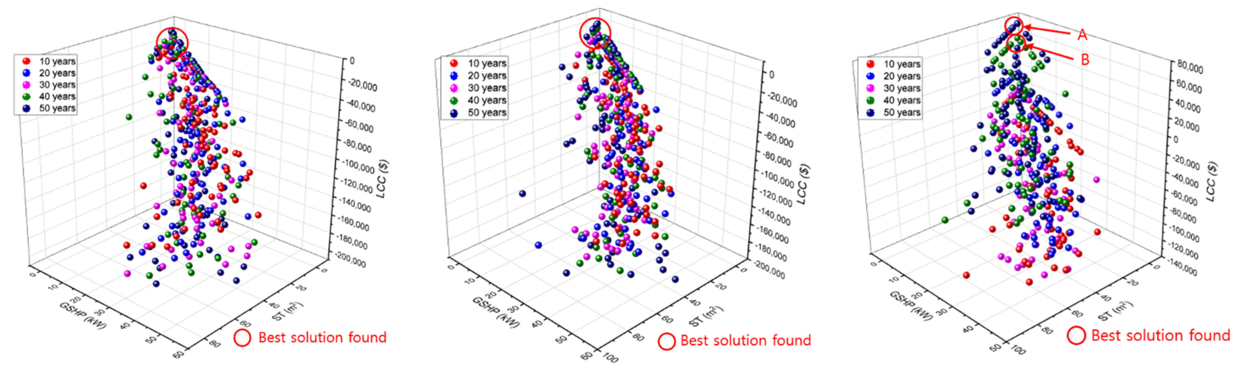
| Years | Scenario 1 | Scenario 2 | Scenario 3 | ||||||
|---|---|---|---|---|---|---|---|---|---|
| ST (m2) | GSHP (kW) | LCC ($) | ST (m2) | GSHP (kW) | LCC ($) | ST (m2) | GSHP (kW) | LCC ($) | |
| 10 years | 0 | 0 | −24,150 | 0 | 0 | −21,900 | 0 | 0 | −4190 |
| 20 years | 0 | 0 | −18,820 | 0 | 0 | −14,520 | 5 | 5 | 120 |
| 30 years | 0 | 0 | −15,140 | 0 | 0 | −8960 | 8 | 0 | 5070 |
| 40 years | 0 | 0 | −10,660 | 0 | 0 | −2760 | 15 | 5 | 33,020 |
| 50 years | 0 | 0 | −7560 | 0 | 0 | 1920 | 28 | 3 | 40,400 |
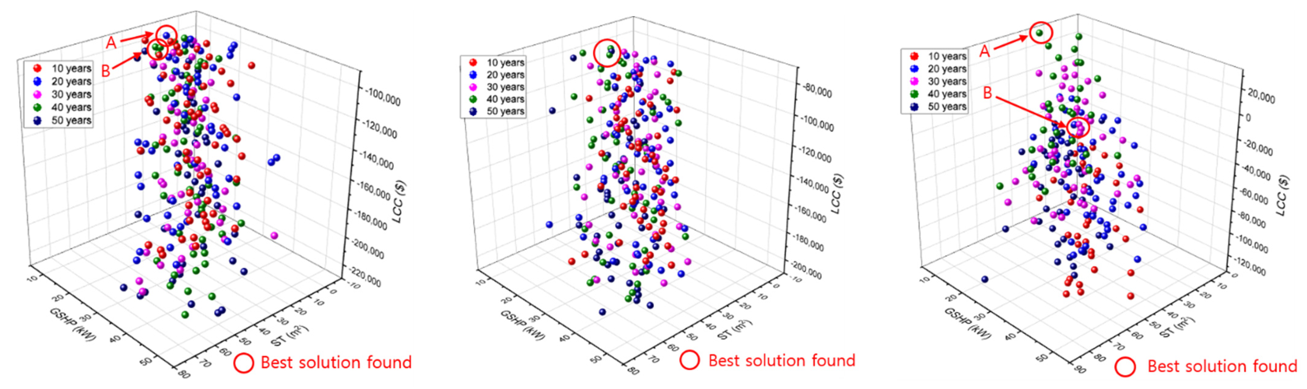
| Years | Scenario 1 | Scenario 2 | Scenario 3 | ||||||
|---|---|---|---|---|---|---|---|---|---|
| ST (m2) | GSHP (kW) | LCC ($) | ST (m2) | GSHP (kW) | LCC ($) | ST (m2) | GSHP (kW) | LCC ($) | |
| 10 years | 26 | 10 | −93,339 | 3 | 20 | −86,490 | 15 | 14 | −54,720 |
| 20 years | 19 | 13 | −91,090 | 12 | 16 | −82,330 | 21 | 11 | −20,470 |
| 30 years | 11 | 17 | −94,370 | 12 | 15 | −80,100 | 21 | 13 | 7750 |
| 40 years | 12 | 15 | −93,000 | 16 | 13 | −77,350 | 28 | 9 | 34,560 |
| 50 years | 0 | 0 | −94,320 | 0 | 0 | −78,650 | 7 | 18 | −42,090 |
| Years | Scenario 1 | Scenario 2 | Scenario 3 | ||||||
|---|---|---|---|---|---|---|---|---|---|
| ST (m2) | GSHP (kW) | LCC ($) | ST (m2) | GSHP (kW) | LCC ($) | ST (m2) | GSHP (kW) | LCC ($) | |
| 10 years | 11 | 19 | −121,240 | 0 | 0 | −75,270 | 9 | 20 | −68,910 |
| 20 years | 18 | 18 | −125,300 | 18 | 16 | −109,400 | 30 | 10 | −17,300 |
| 30 years | 14 | 17 | −120,920 | 8 | 21 | −105,890 | 20 | 15 | 26,180 |
| 40 years | 23 | 14 | −121,470 | 12 | 18 | −98,150 | 19 | 15 | 69,820 |
| 50 years | 18 | 15 | −219,590 | 16 | 17 | −96,280 | 32 | 10 | 105,880 |
Publisher’s Note: MDPI stays neutral with regard to jurisdictional claims in published maps and institutional affiliations. |
© 2021 by the authors. Licensee MDPI, Basel, Switzerland. This article is an open access article distributed under the terms and conditions of the Creative Commons Attribution (CC BY) license (https://creativecommons.org/licenses/by/4.0/).
Share and Cite
Sim, M.; Suh, D.; Otto, M.-O. Multi-Objective Particle Swarm Optimization-Based Decision Support Model for Integrating Renewable Energy Systems in a Korean Campus Building. Sustainability 2021, 13, 8660. https://0-doi-org.brum.beds.ac.uk/10.3390/su13158660
Sim M, Suh D, Otto M-O. Multi-Objective Particle Swarm Optimization-Based Decision Support Model for Integrating Renewable Energy Systems in a Korean Campus Building. Sustainability. 2021; 13(15):8660. https://0-doi-org.brum.beds.ac.uk/10.3390/su13158660
Chicago/Turabian StyleSim, Minjeong, Dongjun Suh, and Marc-Oliver Otto. 2021. "Multi-Objective Particle Swarm Optimization-Based Decision Support Model for Integrating Renewable Energy Systems in a Korean Campus Building" Sustainability 13, no. 15: 8660. https://0-doi-org.brum.beds.ac.uk/10.3390/su13158660