A Machine Learning Approach to Determine Airport Asphalt Concrete Layer Moduli Using Heavy Weight Deflectometer Data

Abstract

An integrated approach based on machine learning and data augmentation techniques has been developed in order to predict the stiffness modulus of the asphalt concrete layer of an airport runway, from data acquired with a heavy weight deflectometer (HWD). The predictive model relies on a shallow neural network (SNN) trained with the results of a backcalculation, by means of a data augmentation method and can produce estimations of the stiffness modulus even at runway points not yet sampled. The Bayesian regularization algorithm was used for training of the feedforward backpropagation SNN, and a k-fold cross-validation procedure was implemented for a fair performance evaluation. The testing phase result concerning the stiffness modulus prediction was characterized by a coefficient of correlation equal to 0.9864 demonstrating that the proposed neural approach is fully reliable for performance evaluation of airfield pavements or any other paved area. Such a performance prediction model can play a crucial role in airport pavement management systems (APMS), allowing the maintenance budget to be optimized.

1. Introduction

Road networks and airport areas are key assets [1] for both developed and developing countries [2]. Maintenance work costs are more significant for developed countries, while first construction work costs are more relevant for developing ones [3]. However, both maintenance and construction work require huge natural resource consumption in terms of aggregates and bituminous binder. In fact, such transport infrastructures have a great impact on energy consumption for the industrial productions involved and the related emissions, given that their service life fixed is in several tens of years [4]. In this regard, the prediction of long-term performance is fundamental, particularly the mechanical strength (stiffness modulus) from repeated investigations over time, in order to properly implement maintenance and rehabilitation (M&R) strategies to achieve sustainable technical, economic, and environmental solutions [5]. It is widely recognized that efficient airport management has positive environmental effects both in reducing major airport congestion and in minimizing land consumption by making a better use of existing infrastructures [6], thus improving the sustainability of airport construction.

The runway is the most important airport infrastructure as it has to ensure adequate operability whatever the traffic and weather conditions. However, there are many causes that can lead to its deterioration such as aging, increased traffic demand, and lack of adequate investment [7]. It is therefore necessary to employ the most suitable and reliable investigation techniques [8] to assess its structural integrity, compliant with the limits of budget constraints [9]. The structural assessment of airport pavements provides valuable information about their expected behavior [10]. It is very useful for estimating their current technical suitability as well as their remaining service life. Moreover, it helps in deciding what rehabilitation strategies to adopt if the frame of a proper airport pavement management system (APMS).

An APMS is based on the concept of preventive maintenance [11,12]: namely, intervening before emergency conditions occur and pavement functionality is compromised. The main purpose of an APMS is to support the managing authority in identifying reliable and cost-effective strategies for preserving the pavement’s proper condition over time. In order to optimize available resources, it is necessary to identify the sections of the pavement that require maintenance, the suitable maintenance solution, the intervention time, and the budget required.

To identify the sections that require structural rehabilitation, pavement structural data is typically obtained through destructive tests on pavement samples, which requires borings, cores, and excavation pits on an existing pavement [13]. These procedures were usually very expensive as they involved subsequent repair of the test pit and could cause the survey area to be closed for several days [14]. Fortunately, hardware and software technology progress has made it possible to replace these procedures with others that are faster and less intrusive, and do not compromise the structural integrity of the pavement. These new approaches, also known as non-destructive tests (NDT) still make it possible to determine the physical and mechanical properties of airport pavement but in a non-destructive manner [15]. For this reason, in recent years, there has been massive use of such tests in the fields of highway and airport pavement evaluation and design [16,17,18,19,20,21,22,23]. Among these NDT methods, the most commonly used for airfield infrastructure condition assessment is the heavy weight deflectometer (HWD) [24]. Similar to the falling weight deflectometer (FWD) which employs smaller loads for highway pavements, the HWD simulates greater aircraft wheel loads [25] and allows for rapid testing of the entire airport pavement so that maintenance and rehabilitation programs can be defined. The deflection basin resulting from the application of the load and measured by means of geophones placed at several distances from the load axis represents an overall system response, namely a good indicator of the pavement’s mechanical behavior. It is also common practice to post-process the deflections measured in order to obtain a significant combination of the deflection basin parameters (DBPs) [26] that even better characterize the structural degradation of the airport pavement [27]. In the literature, the most traditional method to process F/HWD deflections is backcalculation, for pavement layer modulus estimation. Backcalculation is also known as the parameter identification problem, and is basically an optimization process performed to obtain inverse mapping of a known constitutive relationship using discrete or continuous data points [28]. It therefore consists in a numerical analysis of the measured deflections in order to estimate the pavement layer moduli. To achieve this, the measured deflections are matched with the calculated ones. The latter are computed based on the multi-layer elastic (MLE) theory in which stresses and strains are characterized with fourth-order differential equations [29]. In practice, starting from the thickness of the layers, the magnitude of the load and some synthetic moduli (assuming values based on experience and best engineering practices), it is possible to calculate the deflections. Using different sets of moduli, the matching process is iteratively performed until the best match between computed and measured deflections is achieved [30,31,32]. Due to the simplifications introduced by the MLE theory, some studies have observed that the results produced by backcalculation are only acceptable for the pavement surface layer while base and subgrade moduli are often underestimated or overestimated [33]. The fact is that traditional backcalculation software neglect the dynamic effects of F/HWD loadings which, and in order to be implemented would require major model complexity, with consequent huge computational costs [34].

In recent years, several optimization techniques such as genetic algorithms, data mining, heuristic algorithms, and artificial neural networks (ANNs) have been increasingly used to solve similar issues [35,36]. These functional abstractions of the biological neural structure are particularly suited for hard-to-learn problems without a well-established formal theory for their solution [37]. Although ANNs work on the basis of a non-physically based approach, they are characterized by high computational efficiency and small prediction errors [38]. It is also worth pointing out that with such neural models data processing is very fast, allowing the routine F/HWD deflection analysis to be performed even in the field [39]. However, artificial neural networks usually require a large dataset to be successfully trained. For this reason, starting from multiple finite element simulations, synthetic databases are often prepared and subsequently used as input for the neural models in order to allow its proper training [40]. In this study, the goal was to develop a predictive model which can enhance the conventional backcalculation by means of advanced machine learning features. The result is an innovative soft computing tool that, using state-of-the-art data augmentation techniques and the computational effectiveness of artificial neural networks, can predict reliable values of the runway asphalt concrete modulus (${\mathrm{E}}_{\mathrm{AC}}$), even in points not yet sampled. Since with the proposed approach, it is possible to predict the stiffness modulus by providing as input the deflections and the spatial distribution of the sampling points only, the functional relationship between such variables is respected. Compared to the traditional use of ANNs in the field of pavement engineering, the proposed approach avoids preliminary long finite element simulations for training the model. Therefore, this fast and reliable approach could be used in APMS as a support tool for the planning of intervention priorities.

By providing a numerical estimation of the modulus in an arbitrary location on the runway, the proposed pavement performance prediction model could allow us to identify the areas that most require maintenance interventions thus reducing the costs of instrumental monitoring and consequently allowing active and efficient management [41].

2. Experimental Campaign

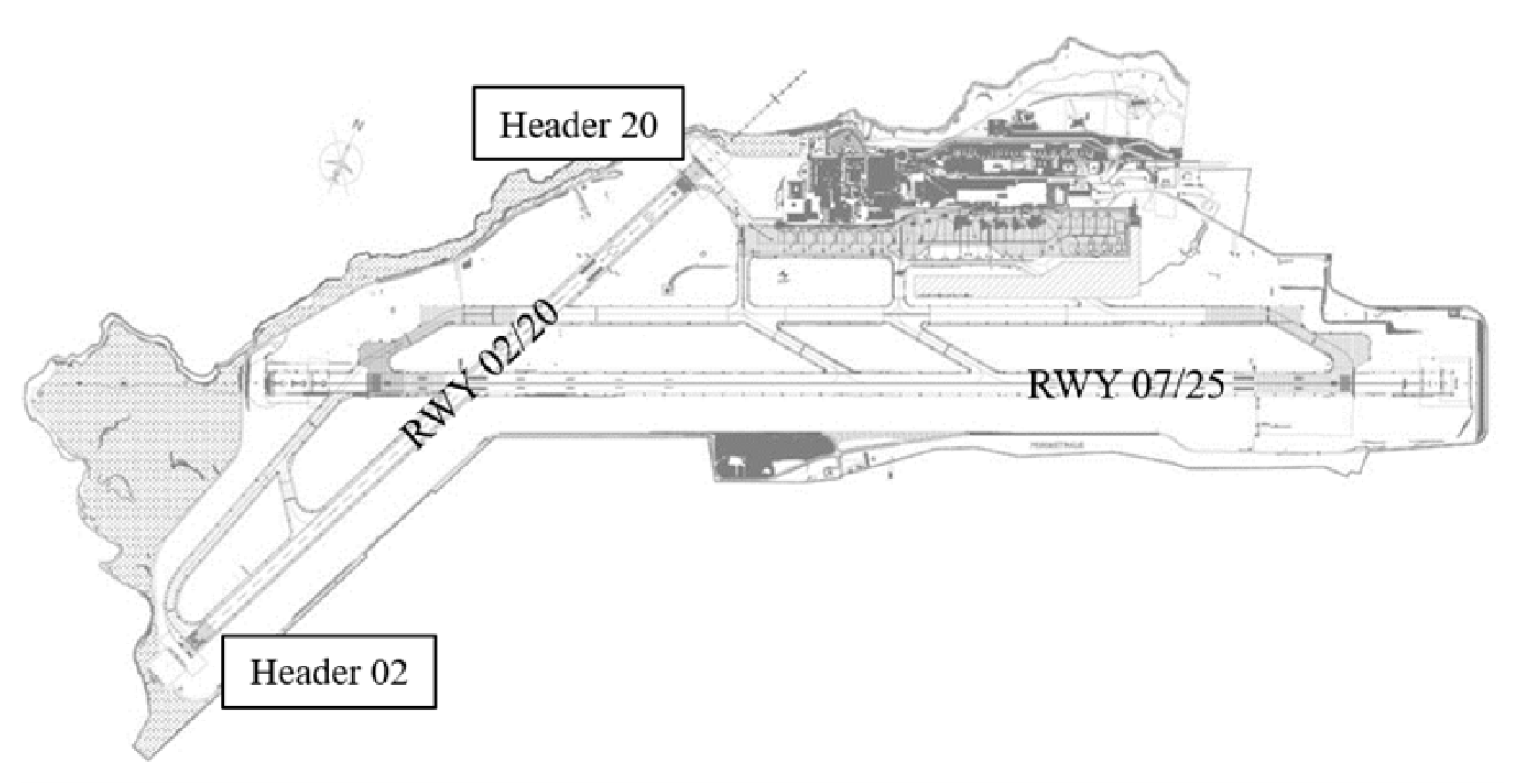
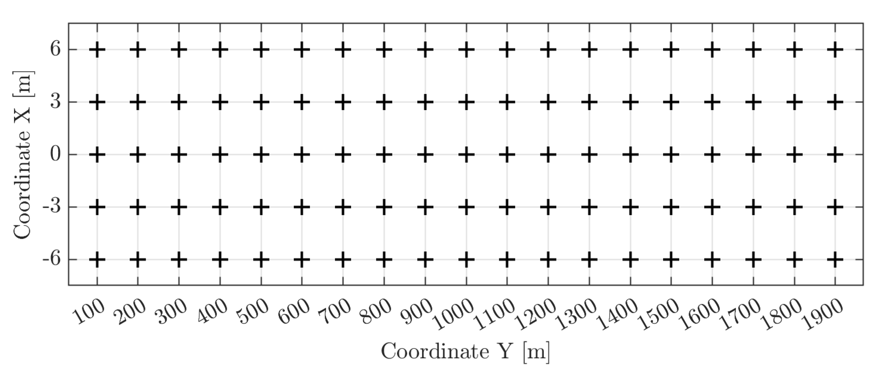
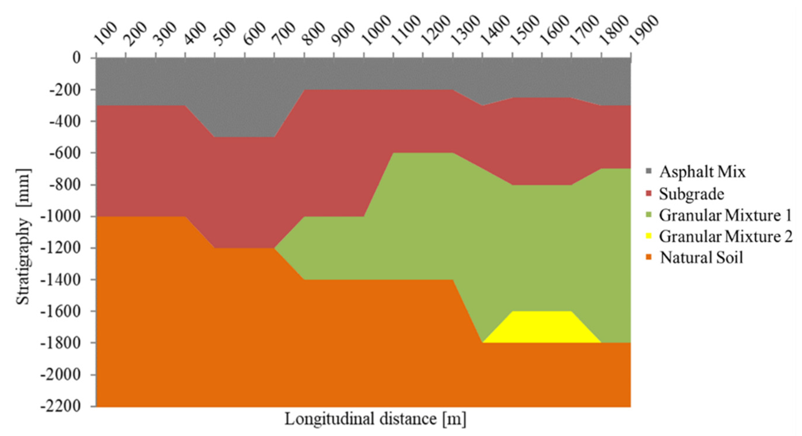
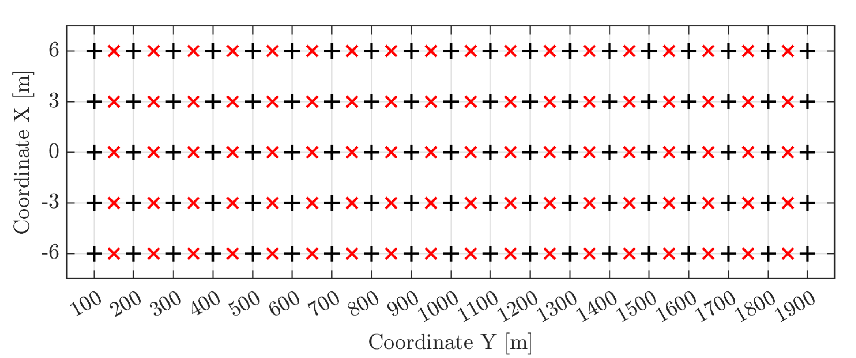
2.1. In Situ Investigation

The experimental campaign took place at the “Falcone e Borsellino” airport of Palermo-Punta Raisi in the period between 9 and 29 February 2012. The Italian international airport is located 35 km west of Palermo. This infrastructure consists of two intersecting runways: the main one named Runway 07/25 and the secondary one named Runway 02/20. On the latter, deflection measurements were collected by means of a heavy weight deflectometer.

Five measurement lines were established: the central axis of the runway (0 m) and other axes ±3 m and ±6 m away from it. The portion of the runway considered, starting from header 02 in the south and arriving at header 20 in the north, was 1800 m long (Figure 1). The experiments were carried out at regular 100 m intervals, thus obtaining 19 impact points for each longitudinal axis. Since there were 5 measurement lines, the total number of measuring points was 95 (Figure 2).

The instrumentation used was the Dynatest 8000, a device capable of performing non-destructive tests and widely used to determine physical and mechanical properties of airport pavements. The principle is to induce small surface deflections of the pavement by applying an impulsive load in a controlled manner. This is done in order to better simulate the effects of an aircraft’s moving wheel [42]. The load is obtained by dropping a suspended mass from a predetermined height on a 30 cm diameter plate resting on the pavement surface. The magnitude of the impulse load transmitted by the device to the pavement can be varied from 30 kN to 240 kN by changing the weight and height of the fall. A magnitude of around 140 kN was adopted. Together with the plate, a set of accelerometric transducers is placed in contact with the pavement and is able to measure the deflections induced at several distances from the loading axis such as 0 (${\mathsf{\delta }}_0$), 200 (${\mathsf{\delta }}_1$), 300 (${\mathsf{\delta }}_2$), 450 (${\mathsf{\delta }}_3$), 600 (${\mathsf{\delta }}_4$), 900 (${\mathsf{\delta }}_5$), 1200 (${\mathsf{\delta }}_6$), 1500 (${\mathsf{\delta }}_7$), and 1800 mm (${\mathsf{\delta }}_8$) from the center of the load. This method is preferred among other methods because it is simpler, more reliable, and cheaper [43]. In fact, the costs that would be associated with reconstructing the area of operation if destructive testing were adopted are avoided [44]. A preliminary contour map of the ${\mathsf{\delta }}_0$ values measured just below the loading plate (Figure 3) immediately shows that the highest deflections are located near the central axis of the pavement. This makes it possible to identify the so-called touchdown zones (TDZs), i.e., those portions of a runway, beyond the threshold, where landing airplanes are first intended to meet the runway [45]. In these areas, ${\mathsf{\delta }}_0$ values exceed 900 $\mathsf{\mu }\mathrm{m}$ and are more than twice or sometimes three times higher than the deflections measured moving away toward the ends of the runway. This provides a preliminary evaluation of which runway areas could require maintenance interventions.

2.2. Deflection Basin Parameters

Deflection basin parameters (DBPs) are obtained by processing the results produced by a HWD investigation and sometimes can be used to monitor the structural integrity of in-service pavements [46]. Based on a comprehensive literature review, the most widely used are:

• Surface curvature index (SCI) which provides information on changes in the near-surface layer’s relative strength.

$$\begin{array}{c}{\mathrm{SCI}}_1={\mathsf{\delta }}_0-{\mathsf{\delta }}_2\\ {\mathrm{SCI}}_2={\mathsf{\delta }}_0-{\mathsf{\delta }}_3\\ {\mathrm{SCI}}_3={\mathsf{\delta }}_0-{\mathsf{\delta }}_4\end{array}$$

(1)

SCI is an accurate indicator of the AC layer conditions and, for certain thicknesses, ${\mathrm{E}}_{\mathrm{AC}}$ and SCI tend to show an approximately linear behavior in a log-log scale [47].

• Deflection ratio (DR) which takes into account the type and quality of materials by relating them to the ratio of two deflections.

$$\mathrm{DR}=\frac{{\mathsf{\delta }}_4}{{\mathsf{\delta }}_0}$$

(2)

• Area under deflection basin curve (AREA) which relates the stiffness of the pavement structure to a shape factor. In fact, it is the partial area under the deflection basin curve normalized with respect to ${\mathsf{\delta }}_0$ using Simpson’s rule [48].

$$\mathrm{AREA}=\frac{150({\mathsf{\delta }}_0+2{\mathsf{\delta }}_2+2{\mathsf{\delta }}_4+{\mathsf{\delta }}_5)}{{\mathsf{\delta }}_0}$$

(3)

This is the definition of the AREA when the deflections are given in millimeters.

• Area under pavement profile (AUPP) [49] which is another indicator sensitive to AC layer properties as found by Thompson and Garg [50].

$$\mathrm{AUPP}=\frac{5{\mathsf{\delta }}_0+2{\mathsf{\delta }}_2+2{\mathsf{\delta }}_4+{\mathsf{\delta }}_5}{{\mathsf{\delta }}_0}$$

(4)

2.3. Backcalculation Process

The Road Moduli Evaluation (RO.M.E.) method was used to determine the elastic moduli of the surface layer impact points. This procedure refers to the multi-layer elastic theory, the Boussinesq-Odemark equation, and the equivalent thickness (E.T.) method. In fact, starting from the thickness measurements of the layers composing the track (obtained from cores and radargrams (Figure 4)) as well as from the FWD results obtained during the experimental campaign, the RO.M.E. method makes it possible to determine the stress/deformation state of each point of the bituminous layer assumed as homogeneous, isotropic, and of semi-infinite thickness. Subsequently, using an iterative procedure, the RO.M.E. method makes the theoretical deflection basin congruent with the experimentally measured one so the pavement layers’ moduli can be estimated. For a complete and comprehensive description of RO.M.E. method operations, please refer to the work of Battiato et al. [51].

Moduli thus backcalculated in Figure 5 make it clear that those areas characterized by the highest deflections (TDZs) show lower modulus values. Similarly, lower deflections are related to higher modulus values. Moreover, the prior determination of the different pavement layers’ thicknesses allowed the identification of homogeneous sections, i.e., those sections of the runway which show the same stratigraphy. A categorical variable that takes into account the homogeneous sections will hereafter be referred to as HS. Backcalculated moduli together with HS have therefore been associated, for each impact point, with the corresponding measured deflections and DBPs. These data will become part of the Input/Target table needed to implement the following supervised learning strategy.

3. Theory and Calculation

3.1. Neural Modeling

An artificial neural network (ANN) is a soft computing technique that takes inspiration from biological neural networks. In this connection, similar to the biological nervous system, such model is constituted by a group of artificial neurons and more or less reinforced interconnections among them. Thus, the artificial neural network is an adaptive system that progressively adapts according to the internal and/or external information learned during the so-called training phase. Its structure, however, does not change over time [52]. Such models are often used to simulate complex relationships between inputs and outputs that other analytic functions cannot represent. Typically, an artificial neural network is organized as a series of layers [53]. Each of them is a collection of neurons and plays a different role. A layer that represents the known data is called the input layer. A layer that produces the network output is called the output layer. All other layers between the input and the output ones are called hidden layers and it is where the computational processing takes place. Here it is necessary to define the activation function, which modulates the amplitude of the output and defines whether or not it should be transmitted to subsequent layers. It is advisable to add more hidden layers as the complexity of the problem to be investigated increases. However, to solve most input–output fitting problems, a single hidden layer with a sufficient number of neurons is adequate [54]. This kind of structure is often called shallow neural network (SNN).

In the current study, three SNNs were examined. The first presents a $4-\mathrm{n}-1$ architecture, the second an $8-\mathrm{n}-1$, whereas the third a $9-\mathrm{n}-1$. The first number represents the neurons composing the input layer (a neuron for every input feature). $\mathrm{n}$ stands for the number of neurons in the hidden layer with $\mathrm{n}$ being an integer in the range $1-30$. Once the first model has been trained and tested (i.e., starting from $\mathrm{n}=1$), a model with $\mathrm{n}+1$ neurons in the hidden layer was iteratively generated until the 30-hidden neurons architecture was obtained. The best hidden activation function for every model was also investigated within a group of four different functions: the exponential linear (ELU), the rectified linear (ReLU), the hyperbolic tangent (TanH), and the logistic sigmoid (LogS). Their analytical expressions together with the resulting graphs are shown in Figure 6. This resulted in a grid-search procedure aimed at identifying the best combination of hidden neurons function guaranteeing the best network performances within the search intervals. Finally, the output layer always consisted of $1$ neuron, and it was associated with a linear activation function.

Each model presented as its input the homogeneous sections (HS) and spatial coordinates of the impact points along the runway $\left(\mathrm{X},\mathrm{Y}\right)$. In addition, the first model added to the feature vector the deflections, ${\mathsf{\delta }}_0$, collected. The second one considered both the ${\mathsf{\delta }}_0$ and all deflections between ${\mathsf{\delta }}_2$ and ${\mathsf{\delta }}_5$. The third one considered the DBPs defined in Section 2.2 instead of individual deflections. The only output was the elastic modulus of the bituminous layer (${\mathrm{E}}_{\mathrm{AC}}$). Even before being assigned to the network, for both inputs and outputs a standardization procedure was provided. This means that each data item was subtracted from its respective mean and divided by its respective standard deviation. This was done because the algorithm chosen to train the network (Bayesian regularization) works best when the inputs and targets are scaled so that they fall approximately in the range of [−1,1] [55].

3.2. Bayesian Regularization

The training process of a neural network consists of applying the sequential steps required to fine-tune synaptic weights and biases in order to generalize the solutions produced by its outputs [56]. In the current study, it started from the Input/Target table mentioned in Section 2.3 and for this reason it is called supervised. The process involves two fundamental steps: a forward and a backward one [57]. The former consists in assigning the feature vector $x$ (i.e., the set of known data) to the network and computing the corresponding output $\widehat{y}$. The latter consists in comparing the generated output with the desired target $y$. The difference between $\widehat{y}$ and $y$ will define the so-called loss function $\mathrm{F}\left(\widehat{y},y\right)$used to determine the corrections to the weights and biases matrix $W$. There are several analytical expressions that define how to update $W$ according to the value assumed by the loss function for a fixed number of iterations $\mathrm{E}$, thus differentiating the several learning algorithms. Usually, the mean squared error (MSE) is used as loss function $\mathrm{F}$. Its analytical expression is presented in Equation (5).

$$\mathrm{MSE}=\frac{1}{\mathrm{n}}{\displaystyle \sum }_1^{\mathrm{n}}{\left({\mathrm{y}}_{\mathrm{i}}-{\hat{\mathrm{y}}}_{\mathrm{i}}\right)}^2$$

(5)

The gradient of the loss function $\mathrm{F}$ with respect to $W$, calculated applying a backpropagation algorithm [58], allows one to update network weights in order to minimize the loss value. Equation (6) shows that the weights at the next iteration $\mathrm{e}+1$ are calculated starting from those used at the previous one $\forall \mathrm{e}\in \left\{1,\dots ,\mathrm{E}\right\}$:

$$W^{\mathrm{e}+1}=W^{\mathrm{e}}-{({\nabla }^2\mathrm{F}\left(W^{\mathrm{e}}\right))}^{-1}\nabla \mathrm{F}\left(W^{\mathrm{e}}\right)$$

(6)

Combining this with the Levenberg–Marquardt (LM) backpropagation algorithm [59] results in:

$$W^{\mathrm{e}+1}=W^{\mathrm{e}}-{[J^{\mathrm{T}}\left(W^{\mathrm{e}}\right)J\left(W^{\mathrm{e}}\right)+{\mathsf{\mu }}_{\mathrm{e}}I]}^{-1}{J}^{\mathrm{T}}\left(W^{\mathrm{e}}\right)v\left(W^{\mathrm{e}}\right)$$

(7)

where $W$ is the matrix of weights and biases, $J$ is the Jacobian matrix of the training loss function $\mathrm{F}$ with respect to $W^{\mathrm{e}}$, $I$ is the identity matrix, whereas $v$ is the vector of the network errors obtained through the expression:

$$v(W^{\mathrm{e}})=\widehat{y}(W^{\mathrm{e}})-y$$

(8)

The scalar $\mathsf{\mu }$ (also known as “learning rate”) defines the algorithm convergence rate. As $\mathsf{\mu }$ is increased, the LM algorithm moves toward a small step in the direction of steepest descent $J^{\mathrm{T}}\left(W^{\mathrm{e}}\right)v\left(W^{\mathrm{e}}\right)$. Instead, if $\mathsf{\mu }$ is decreased, convergence will be faster with the possibility that the algorithm may jump over the minimum. For this reason, during the training phase, the $\mathsf{\mu }$ value is modified to reach convergence as quickly as possible avoiding undesirable local minima. An initial value of $\mathsf{\mu }$ is set for the first step. Subsequently it increases (or decreases) being multiplied by a factor ${\mathsf{\mu }}_{\mathrm{inc}}>1$ (or ${\mathsf{\mu }}_{\mathrm{dec}}<1$) if the previous iteration led to worse (or better) results in terms of the loss function F. In this way, the loss function tends to gradually decrease step by step. Finally, it is necessary to set a maximum value of $\mathsf{\mu }$ (indicated by ${\mathsf{\mu }}_{\max }$) in order to interrupt the training if it is exceeded. When ${\mathsf{\mu }}_{\max }$ has been reached (or alternatively at the end of the $\mathrm{E}$ iterations) the best weights and biases are identified and kept fixed. Then the test feature vector is assigned as input making the network work only in the forward manner thus determining the model’s loss index on some data never processed before. However, working this way, it is possible to run into a phenomenon known in machine learning as “overfitting”. Overfitting occurs when the model performs very well with the given training set of observations but cannot generalize correctly beyond it and consequently performs very poorly with test data or different sets of observations [60]. This often occurs when the connection weights’ values are too high. For this reason, in the current study, it was decided to use a regularization technique considering the matrix $W$ values. This technique consists in no longer rewriting the loss function as MSE but as follows:

$${\mathrm{F}}_{\mathrm{opt}}\left(\widehat{y}(W^{\mathrm{e}}\right),y,W^{\mathrm{e}})=\mathsf{\beta }\Vert \widehat{y}(W^{\mathrm{e}})-y{\Vert }_{\mathbf{2}}^{\mathbf{2}}+\mathsf{\alpha }\Vert W^{\mathrm{e}}{\Vert }_2^2$$

(9)

The $\Vert ·{\Vert }_2^2$ operator represents the 2-norm, and it is applied first to the errors $v(W^{\mathrm{e}})=\widehat{y}(W^{\mathrm{e}})-y$and then to network parameters $W^{\mathrm{e}}$. For this reason, the first term is also known as the sum squared error (SSE) while the second term represents a correction that considers the complexity of the network through its weights (also known as “penalty”). In addition, both terms are pre-multiplied by parameters indicated as $\mathsf{\beta }$ and $\mathsf{\alpha }$ whose ratio defines the smoothness of the loss function. The larger the ratio $\mathsf{\alpha }/\mathsf{\beta }$ is, the smoother the network response will be. This concept was first introduced by Tikhonov [61]. The penalty term (also referred to as “regularization”) forces the resulting loss function to be smooth. When the weights are large, the loss function can have large slopes and is therefore more likely to overfit the training data. On the other hand, if the weights are forced to be small, the loss function will smoothly interpolate the training data, thus achieving good performance even beyond the training set. The correct choice of the regularization ratio $\mathsf{\alpha }/\mathsf{\beta }$ is essential in producing a network that generalizes properly. In this study, it was decided to use David MacKay’s approach [62] to correctly define the regularization terms. This approach involves an early initialization of the $\mathsf{\alpha }$ and $\mathsf{\beta }$ parameters (as well as the network weights). Using Bayesian statistical and optimization techniques, $\mathsf{\alpha }$ and $\mathsf{\beta }$ values are varied at each iteration thus changing the loss function and obviously its minimum point. Generally, each time a new minimum is set, the regularization parameters are more accurate. Eventually, the precision will be high enough that the objective function will no longer significantly change with every subsequent iteration and convergence will therefore have been achieved. The default values of the hyperparameters implemented in the MATLAB^® Toolbox LM algorithm ($\mathsf{\mu },{\mathsf{\mu }}_{\mathrm{inc}},{\mathsf{\mu }}_{\mathrm{dec}},{\mathsf{\mu }}_{\max }$ and $\mathrm{E}$) were used, namely the initial $\mathsf{\mu }$ was set equal to 0.001, ${\mathsf{\mu }}_{\mathrm{inc}}$ to 10, ${\mathsf{\mu }}_{\mathrm{dec}}$ to 0.1, ${\mathsf{\mu }}_{\max }$ to $1\times {10}^{10}$, whereas the maximum number of training epochs $\mathrm{E}$ was 1000. As explained in Section 3.1, the size of the hidden layer together with its activation function were identified by performing a grid search. Moreover, one last parameter, ${\mathrm{w}}_{\mathrm{w}}$, was defined. It represented the number of re-trainings performed for each iteration and was set equal to 10. This was done in order to obtain the best network among the 10 fitted networks for every combination of neurons function as a result of a k-fold cross-validation partitioning.

3.3. K-Fold Cross-Validation

Together with the standardization procedure explained in Section 3.1, a further data pre-processing step was implemented. Usually, the dataset is simply split into two partitions: one for training and the other for testing. This method, also known as “hold-out”, produces errors in the test phase with very variable results depending on which observations have ended up in one partition or another [63]. This undesirable effect is even more pronounced when the dataset is particularly limited so, to overcome this problem, the $\mathrm{k}$-fold cross-validation (CV) was adopted [64]. This technique depends on a single parameter $\mathrm{k}$, an index of the number of partitions into which the dataset must be divided. After randomly mixing the known data, a value of $\mathrm{k}$ is established and consequently the dataset is divided into $\mathrm{k}$ groups each containing the same number of elements. In this way, $\mathrm{k}-1$ groups are used to build the model and the left-out sample to validate it Figure 7. This is an iterative procedure that is repeated $\mathrm{k}$-times so that each of the $\mathrm{k}$-folds is successively assigned as validation data [65].

For each iteration, a validation score is tracked and recorded before moving on to the next iteration. The average of the obtained $\mathrm{k}$-validation scores is assumed as the general performance of the model [66]:

$$\mathrm{Val}.{\mathrm{Score}}_{\mathrm{CV}}=\frac{1}{\mathrm{n}}{\displaystyle \sum }_1^{\mathrm{n}}\mathrm{Val}.{\mathrm{Score}}_{\mathrm{i}}$$

(10)

A review of model validation methods recommends $\mathrm{k}$-fold cross-validation, particularly five or ten-fold [67]. The value of $\mathrm{k}$ has therefore been set equal to five, to remain consistent with the relevant literature [68]. Because of the five-fold CV, the dataset is split as follows: 80% of the available data for the training set and 20% for the test set.

3.4. Data Augmentation

In the context of machine learning, whenever a certain technique is used to expand the size of the starting dataset, a data augmentation technique is used. This is a generation of synthetic data that comes from data processing and not from a new experimental campaign. In this sense, increasing the amount of data available to the network increases its predictive capabilities by improving its generalization. Data augmentation techniques are particularly popular in the field of image classification because rotating, zooming, cropping, or changing the brightness does not mean changing the information stored in an image. Similarly, in the case of time-series data augmentation it is necessary to use techniques that do not disturb the information collected during the experimental campaign but, at the same time, allow one to increase the sample size. Since collecting new data can be very expensive and time-consuming, multiple interpolation techniques are progressively emerging in data augmentation. Interpolation is a method of estimating unknown values using known data. More precisely, if the function $\mathrm{f}\left(\mathrm{x}\right)$ of the real variable $\mathrm{x}$ is unknown and the function value $\mathrm{f}\left({\mathrm{x}}_{\mathrm{i}}\right)$ for the value ${\mathrm{x}}_{\mathrm{i}}\left(\mathrm{i}=1,2,\dots ,\mathrm{n}\right)$ of two or more variables with a certain interval is known, estimating a function value for any $\mathrm{x}$ in between is called interpolation [69]. As suggested by Oh et al. [70], the known dataset should never be shorter but rather longer than the one obtained through interpolation. For this reason, it was decided to nearly double the initial dataset by interpolating the unknown bidimensional function at a midpoint between two successive impact points of the same measuring line (Figure 8).

The function chosen as interpolator becomes a kind of model hyperparameter. The proposed method used the modified Akima interpolation, often known as the “makima” technique. In general, the Akima algorithm performs cubic interpolation to produce piecewise polynomials with continuous first-order derivatives [71]. Unlike 3rd degree polynomial or cubic spline interpolation, the Akima algorithm avoids excessive local undulations while still being able to deal with oscillatory data. The modified Akima algorithm (i.e., “makima”) is an extension of the method just mentioned and it is designed for interpolating values given at points of a rectangular grid in a plane by a smooth bivariate function $\mathrm{z}=\mathrm{z}\left(\mathrm{x},\mathrm{y}\right)$. The interpolating function is therefore a bicubic polynomial in each cell of the rectangular grid [72]. The main purpose is still to produce fewer undulations between given grid points. Data obtained through makima interpolation (85 augmented points) were used exclusively during the model training phase and were added to the $\mathrm{k}$-fold partitioning for a total of 161 training points.

Assuming as current state-of-practice (CSP) the ANN model implemented in MATLAB^® Toolbox, the comparison between this simplified model and the one proposed by the authors has been considered. Such comparison allows one to evaluate the improvement of stiffness values estimation given by the proposed model. Moreover, assuming that data augmentation implementation is nearly equivalent to a denser experimental campaign, it can be understood how the change of the HWD measurements resolution affects the modeling result.

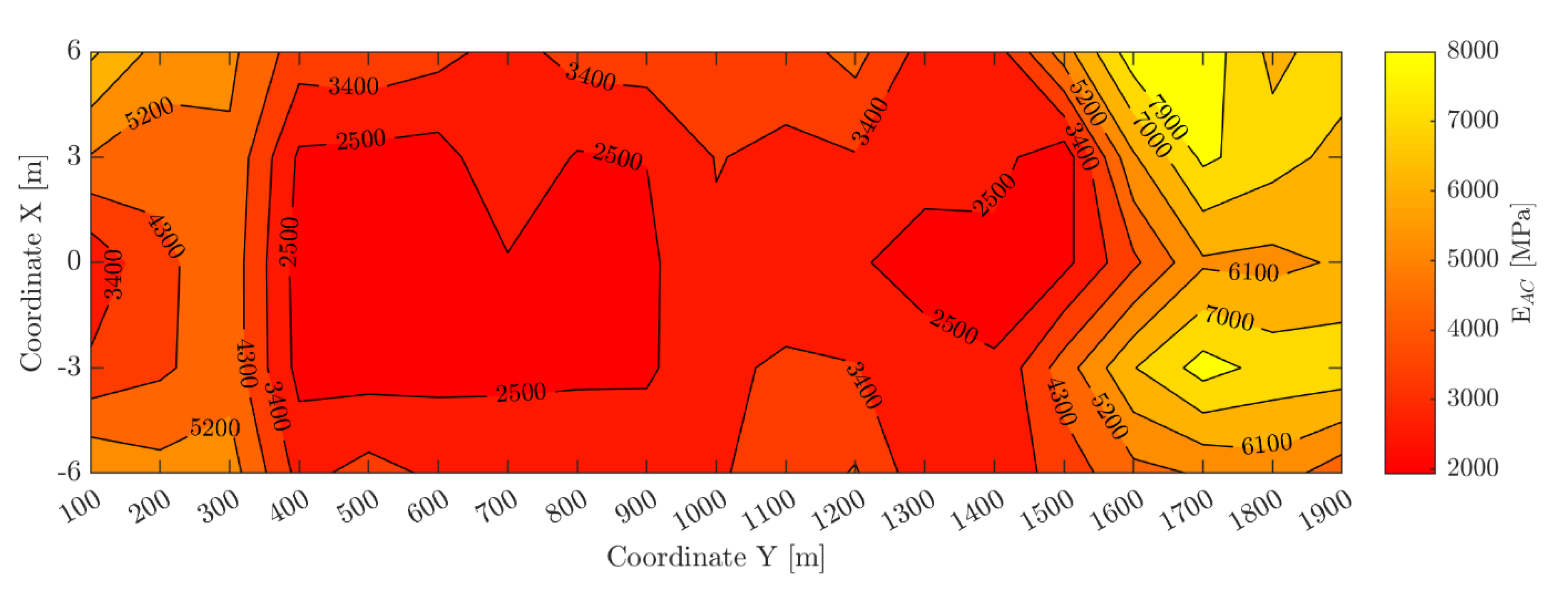
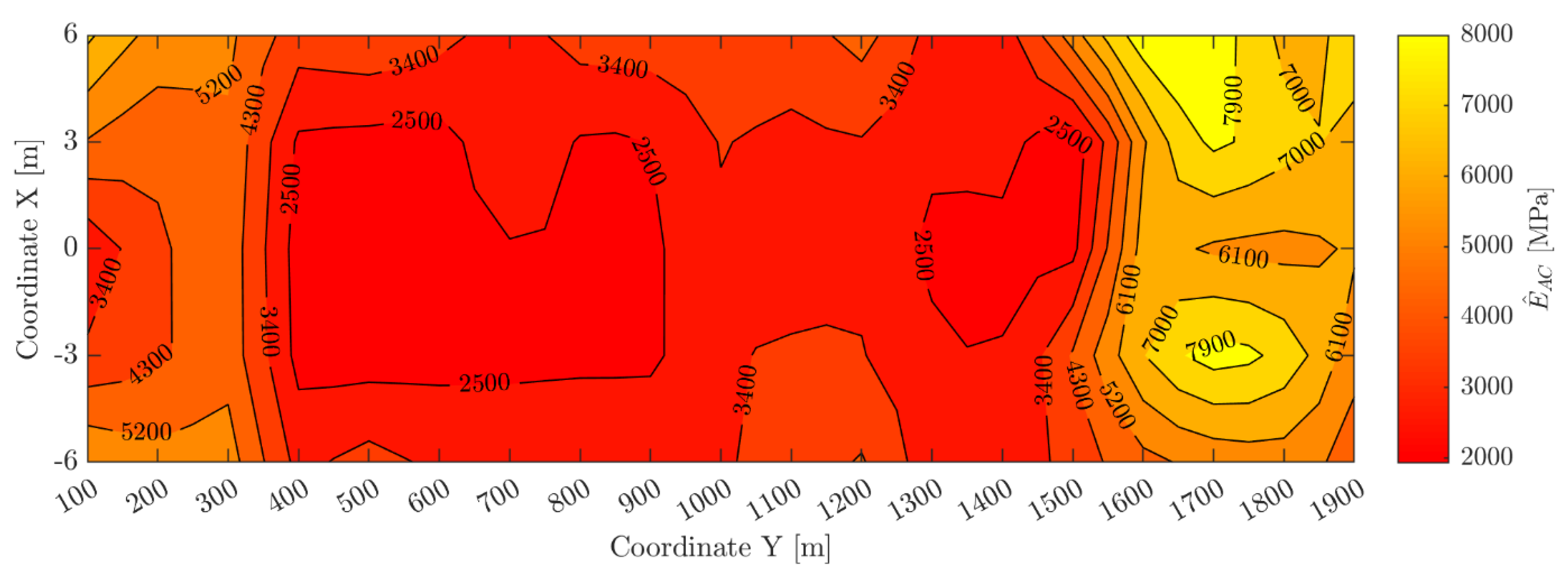
4. Results and Discussion

Although the starting dataset is highly variable both in terms of measured deflections and backcalculated moduli along the runway (due to the pronounced differences in mechanical behavior), the proposed neural model returns very satisfactory results (

Table 1. Summary results of the first model.

Inputs	Output	Activation Fun.	Best Architecture	$\mathbf{R}$	$\mathbf{M}\mathbf{S}\mathbf{E}$	${\mathbf{R}}_{\mathbf{a}\mathbf{d}\mathbf{j}}^2$
δ0, HS, X, Y	${\mathrm{E}}_{\mathrm{AC}}$	ELU	4-12-1	0.9673	0.0682	0.9231
		ReLU	4-27-1	0.9408	0.1309	0.8627
		TanH	4-25-1	0.9780	0.0494	0.9477
		LogS	4-22-1	0.9772	0.0474	0.9461

,

Table 2. Summary results of the second model.

Inputs	Output	Activation Fun.	Best Architecture	$\mathbf{R}$	$\mathbf{M}\mathbf{S}\mathbf{E}$	${\mathbf{R}}_{\mathbf{a}\mathbf{d}\mathbf{j}}^2$
δ0, δ2, δ3, δ4, δ5, HS, X, Y	${\mathrm{E}}_{\mathrm{AC}}$	ELU	8-27-1	0.9805	0.0423	0.9368
		ReLU	8-3-1	0.9455	0.1217	0.8277
		TanH	8-9-1	0.9806	0.0437	0.9370
		LogS	8-13-1	0.9844	0.0370	0.9493

and

Table 3. Summary results of the third model.

Inputs	Output	Activation Fun.	Best Architecture	$\mathbf{R}$	$\mathbf{M}\mathbf{S}\mathbf{E}$	${\mathbf{R}}_{\mathbf{a}\mathbf{d}\mathbf{j}}^2$
SCI1, SCI2, SCI3, DR, AUPP, AREA, HS, X, Y	${\mathrm{E}}_{\mathrm{AC}}$	ELU	9-18-1	0.9804	0.0501	0.9303
		ReLU	9-14-1	0.9555	0.0963	0.8441
		TanH	9-26-1	0.9807	0.0439	0.9312
		LogS	9-23-1	0.9864	0.0321	0.9516

). The performance of the model is expressed in terms of Pearson coefficient $\mathrm{R}$, mean squared error $\mathrm{MSE}$, and adjusted coefficient of determination ${\mathrm{R}}_{\mathrm{adj}}^2$. The first one expresses, if any, a linear correlation between the backcalculated moduli ${\mathrm{E}}_{\mathrm{AC}}$ and those predicted by the neural model ${\widehat{\mathrm{E}}}_{\mathrm{AC}}$:

$$\mathrm{R}({\mathrm{E}}_{\mathrm{AC}},{\widehat{\mathrm{E}}}_{\mathrm{AC}})=\frac{1}{\mathrm{n}-1}{\displaystyle \sum }_{\mathrm{i}=1}^{\mathrm{n}}\left(\frac{{\mathrm{E}}_{{\mathrm{AC}}_{\mathrm{i}}}-{\mathsf{\mu }}_{{\mathrm{E}}_{\mathrm{AC}}}}{{\mathsf{\sigma }}_{{\mathrm{E}}_{\mathrm{AC}}}}\right)\left(\frac{{\widehat{\mathrm{E}}}_{{\mathrm{AC}}_{\mathrm{i}}}-{\mathsf{\mu }}_{{\widehat{\mathrm{E}}}_{\mathrm{AC}}}}{{\mathsf{\sigma }}_{{\widehat{\mathrm{E}}}_{\mathrm{AC}}}}\right)$$

(11)

where $\mathsf{\mu }$ and $\mathsf{\sigma }$ are the mean and the standard deviation of the variables, respectively. Values of $\mathrm{R}$ exceeding 0.8 are typical of a satisfactory correlation [73,74]. The second provides an accurate estimation of the model generalization capability by averaging the squares of the differences between backcalculated and predicted moduli:

$$\mathrm{MSE}({\mathrm{E}}_{\mathrm{AC}},{\widehat{\mathrm{E}}}_{\mathrm{AC}})=\frac{1}{\mathrm{n}}{\displaystyle \sum }_{\mathrm{i}=1}^{\mathrm{n}}{({\mathrm{E}}_{{\mathrm{AC}}_{\mathrm{i}}}-{\widehat{\mathrm{E}}}_{{\mathrm{AC}}_{\mathrm{i}}})}^2$$

(12)

The third one represents in what percentage the input variables can explain a variation of the output variable:

$${\mathrm{R}}_{\mathrm{adj}}^2({\mathrm{E}}_{\mathrm{AC}},{\widehat{\mathrm{E}}}_{\mathrm{AC}})=1-\left(\frac{\mathrm{n}-1}{\mathrm{n}-\mathrm{p}}\right)\frac{\mathrm{SSE}}{\mathrm{SST}}$$

(13)

where $\mathrm{SSE}={\displaystyle \sum }_{\mathrm{i}=1}^{\mathrm{n}}{\left({\mathrm{E}}_{{\mathrm{AC}}_{\mathrm{i}}}-{\widehat{\mathrm{E}}}_{{\mathrm{AC}}_{\mathrm{i}}}\right)}^2$ is the sum of squared error, $\mathrm{SST}={\displaystyle \sum }_{\mathrm{i}=1}^{\mathrm{n}}{\left({\mathrm{E}}_{{\mathrm{AC}}_{\mathrm{i}}}-{\mathsf{\mu }}_{{\mathrm{E}}_{\mathrm{AC}}}\right)}^2$ is the sum of squared total, $\mathrm{n}$ is the number of observations, and $\mathrm{p}$ is the number of model inputs. Its formulation allows one to understand whether adding more independent variables will improve the goodness-of-fit for the regression model. In fact, the adjusted $\mathrm{R}$-squared score increases when new terms improve the model fit while decreases when this improvement is not appreciable.

For what concerns the grid search approach, among the possible combinations of hidden neurons-activation function, the one that maximized the ${\mathrm{R}}_{\mathrm{adj}}^2$ was chosen. The intention was to produce a network that would make small errors and, at the same time, make the best use of the parameters provided as input. From this point of view, the model that produced the best results is the third one. The architecture $9-23-1$ with logistic sigmoid activation function (hereafter referred to as LogS-SNN) has produced a ${\mathrm{R}}_{\mathrm{adj}}^2$ value equal to 0.9516, confirming that the DBPs, together with the homogeneous sections and the spatial coordinates of the impact points, are very suitable starting data to make modulus predictions. The graphical trend of $\mathrm{R}$ and $\mathrm{MSE}$ is shown in Figure 9a for a clearer appreciation of the learning process. It is important to notice how the former increases up to the best value and then settles around constant values. Similarly, the latter decreases down to the best value and then settles around constant values. This is the representation of the happened learning process. Adding more hidden neurons beyond the threshold of the best value would computationally weigh down the model without leading to any benefit in predictive terms.

As further evidence of the network efficiency from the computational cost point of view, another parameter was kept under observation: the effective number of parameters ($\mathrm{ENP}$). It provides a measure of how many parameters (weights and biases) in the neural model are effectively used in reducing the loss function [59]. The $\mathrm{ENP}$ is expressed by:

$$\mathrm{ENP}={\displaystyle \sum }_{\mathrm{i}=1}^5\frac{{\mathsf{\gamma }}_{\mathrm{i}}-2{\mathsf{\alpha }}_{\mathrm{i}}\mathrm{tr}({\nabla }^2\mathrm{F}\left(W_{\mathrm{i}}\right)}{{\mathsf{\gamma }}_{\mathrm{i}}}$$

(14)

where $W_{\mathrm{i}}$ is the matrix of weights and biases of the $\mathrm{i}$-th SNN model trained during the $\mathrm{k}$-fold cross-validation procedure and ${\mathsf{\gamma }}_{\mathrm{i}}$ is the total number of parameters of the same $\mathrm{i}$-th SNN. The trace of the Hessian matrix can be computed starting from the Jacobian matrix of the training set errors and the parameters ${\mathsf{\alpha }}_{\mathrm{i}}$ and ${\mathsf{\beta }}_{\mathrm{i}}$, as explained by Hagan et al. [59]. With a ratio of 185/254, the LogS-SNN $\mathrm{ENP}$ shows that, despite the large number of neurons within the hidden layer, more than 70% of the model’s parameters are used to reduce the loss function. It is probably the ideal combination of computational efficiency and accuracy in the predictions as also highlighted by the value of mean squared error ${\mathrm{MSE}}_{\mathrm{CV}}$equal to 0.0321. For a complete illustration of the results, the performance of the LogS-SNN model for each of the five folds has been graphically represented Figure 9b. As explained in Section 3.3, averaging the results over the five folds, the predictive capabilities of the model can be evaluated resulting in a ${\mathrm{R}}_{\mathrm{CV}}$ equal to 0.9864. Using a VivoBookProN580GD-FI018T with Intel(R) core(TM) i7-8750H CPU @2.20 GHz and 16 GB RAM, this model takes 13 s to process the data. The LogS-SNN model finally made it possible to predict the modulus value at each point of the runway thus generating a contour map (Figure 10). From a comparison with the map in Section 2.3, it can be concluded that the neural modeling procedure followed was successful in fitting the presented experimental data. The contour map provides a quantitative estimation of the pavement mechanical performance at the time of the HWD experimental investigations.

It is worth pointing out that a simple interpolation of the backcalculated modulus data can certainly estimate the value of ${\mathrm{E}}_{\mathrm{AC}}$ at any point on the runway, but it would predict the stiffness without any phenomenological relationship being considered. On the other hand, the proposed neural model predicts the AC modulus value at any point on the pavement but requires the measured deflections, their coordinates along the runway, and the stratigraphy as input. This approach preserves the fundamental relationship between the modulus and the mentioned variables, from a logical point of view.

5. Conclusions

This paper was focused on prediction of the stiffness modulus of a runway pavement AC layer, a critical element in pavement management, by means of an innovative methodological approach based on soft computing techniques, namely machine learning and data augmentation. Specifically, shallow neural networks, characterized by a three-layer architecture, and the modified Akima algorithm were adopted. The results of an experimental trial carried out on Runway 02/20 at Palermo airport by means of HWD, were used to develop three different predictive SNN models.

The spatial coordinates of the impact points and a categorical variable representative of the pavement section type were always included in the model’s input vector. In addition to such variables, the first SNN model considered the measure ${\mathsf{\delta }}_0$. In the second predictive model, all deflections between ${\mathsf{\delta }}_2$ and ${\mathsf{\delta }}_5$ were also included. In the third and last neural model, the deflection measurements were replaced by the deflection basin parameters.

To optimize the number of hidden neurons and to select the best suited type of activation function, a grid search was carried out. Bayesian regularization algorithms and a k-fold cross-validation procedure was implemented in order to identify the model characterized by the best predictive performance.

The results showed that the best performing SNN model is the third one, characterized by 23 neurons in the hidden layer and a logistic sigmoid activation function. This model can produce very accurate stiffness modulus predictions with $\mathrm{R}$ and $\mathrm{MSE}$ values equal to 0.9864 and 0.0321, respectively. Moreover, in order to consider both the size of the available dataset and the number of parameters, the ${\mathrm{R}}_{\mathrm{adj}}^2$ evaluation metric has been used; its value, equal to 0.9516, has fully confirmed the good performance of the predictive model.

The elaboration of the data by means of CSP ANN model produced a Pearson correlation coefficient equal to 0.9460. Conversely, thanks to the implementation of a data augmentation technique, the proposed model produces more accurate predictions. The R-value is equal to 0.9864, resulting in a 4% increase in the correlation coefficient.

The proposed soft computing approach, which is proven to be able to predict the stiffness modulus at any point on the runway, can become a crucial element in APMS, thus allowing optimization of the available maintenance budget, in order to improve safety and sustainability of airport infrastructures.

The proposed approach has been developed with respect to the Palermo runway, but it could be easily adopted to analyze any runway or paved area such as parking lots. So far, the study does not consider historical series of deflections: it would be interesting to implement this additional information in order to evaluate if the presented methodology is suitable not only for evaluating the current pavement deterioration state, but for predicting its evolution and scheduling intervention priorities over time as well.

References

1. Moteff, J.; Parfomak, P. Critical Infrastructure and Key Assets: Definition and Identification; Library of Congress Washington DC Congressional Research Service: Washington, DC, USA, 2004. [Google Scholar]
2. Schweikert, A.; Chinowsky, P.; Espinet, X.; Tarbert, M. Climate change and infrastructure impacts: Comparing the impact on roads in ten countries through 2100. Procedia Eng. 2014, 78, 306–316. [Google Scholar] [CrossRef] [Green Version]
3. Makovšek, D.; Tominc, P.; Logožar, K. A cost performance analysis of transport infrastructure construction in Slovenia. Transportation 2012, 39, 197–214. [Google Scholar] [CrossRef]
4. Navneet, G.; Guo, E.; McQueen, R. Operational Life of Airport Pavements; Federal Aviation Administration: Washington, DC, USA, 2004. [Google Scholar]
5. Ashtiani, A.Z.; Murrell, S.; Brill, D.R. Machine Learning Approach to Identifying Key Environmental Factors for Airfield Asphalt Pavement Performance. In Airfield and Highway Pavements 2021, Virtual Conference, 8–10 June 2021; American Society of Civil Engineers: Reston, VA, USA, 2021; pp. 328–337. [Google Scholar]
6. Carlucci, F.; Cirà, A.; Coccorese, P. Measuring and explaining airport efficiency and sustainability: Evidence from Italy. Sustainability 2018, 10, 400. [Google Scholar] [CrossRef] [Green Version]
7. Rix, G.J.; Baker, N.C.; Jacobs, L.J.; Vanegas, J.; Zureick, A.H. Infrastructure assessment, rehabilitation, and reconstruction. In Proceedings of the Frontiers in Education 1995 25th Annual Conference. Engineering Education for the 21st Century, Atlanta, GA, USA, 1–4 November 1995; IEEE: New York, NY, USA, 1995; Volume 2, pp. 4c1–11. [Google Scholar]
8. Zou, L.; Yi, L.; Sato, M. On the use of lateral wave for the interlayer debonding detecting in an asphalt airport pavement using a multistatic GPR system. IEEE Trans. Geosci. Remote Sens. 2020, 58, 4215–4224. [Google Scholar] [CrossRef] [Green Version]
9. Guo, Y.; He, X.; Peeta, S.; Weiss, W.J. Internal curing for concrete bridge decks: Integration of a social cost analysis in evaluation of long-term benefit. Transp. Res. Rec. 2016, 2577, 25–34. [Google Scholar] [CrossRef]
10. Haas, R.; Hudson, W.R.; Zaniewski, J.P. Modern Pavement Management; Krieger Publishing Company: Melbourne, FL, USA, 1994. [Google Scholar]
11. Zheng, M.; Chen, W.; Ding, X.; Zhang, W.; Yu, S. Comprehensive life cycle environmental assessment of preventive maintenance techniques for asphalt pavement. Sustainability 2021, 13, 4887. [Google Scholar] [CrossRef]
12. De Souza, N.M.; De Almeida Filho, A.T. A systematic airport runway maintenance and inspection policy based on a delay time modeling approach. Autom. Constr. 2020, 110, 103039. [Google Scholar] [CrossRef]
13. Chern, S.G.; Lee, Y.S.; Hu, R.F.; Chang, Y.J. A research combines nondestructive testing and a neuro-fuzzy system for evaluating rigid pavement failure potential. J. Mar. Sci. Technol. 2005, 13, 133–147. [Google Scholar]
14. Huang, Y.H. Pavement Analysis and Design; Prentice-Hall: Englewood Cliffs, NJ, USA, 1993. [Google Scholar]
15. Hoffman, M. Comparative study of selected nondestructive testing devices. Transp. Res. Rec. 1982, 852, 32–41. [Google Scholar]
16. ASTM. ASTM D4695. Standard Test Method for Deflections with A Falling Weight-Type Impulse Load Device; ASTM: West Conshohocken, PA, USA, 1996. [Google Scholar]
17. ASTM. ASTM D5340. Standard Test Method for Airport Pavement Condition Index Survey; ASTM: West Conshohocken, PA, USA, 1996. [Google Scholar]
18. ASTM. ASTM D4695-96. Standard Guide for General Pavement Deflection Measurement; ASTM: West Conshohocken, PA, USA, 1996. [Google Scholar]
19. Sebaaly, B.E.; Mamlouk, M.S.; Davies, T.G. Dynamic analysis of falling weight deflectometer data. Transp. Res. Rec. 1986, 1070, 63–68. [Google Scholar]
20. Bush III, A.J.; Alexander, D.R. Pavement evaluation using deflection basin measurements and layered theory. Transp. Res. Rec. 1985, 1022, 16–29. [Google Scholar]
21. Chang, D.W.; Kang, Y.V.; Roesset, J.M.; Stokoe, K. Effect of depth to bedrock on deflection basins obtained with Dynaflect and falling weight deflectometer tests. Transp. Res. Rec. 1992, 1355, 8–16. [Google Scholar]
22. Ullidtz, P.; Coetzee, N. Analytical procedures in nondestructive testing pavement evaluation. Transp. Res. Rec. 1995, 1482, 61–66. [Google Scholar]
23. Weil, G.J. Non-destructive testing of bridge, highway and airport pavements. In Proceedings of the Fourth International Conference of Ground Penetrating Radar, Rovaniemi, Finland, 8–13 June 1992; European Association of Geoscientists & Engineers: Utrecht, The Netherlands, 1992; pp. 259–266. [Google Scholar]
24. Gopalakrishnan, K. Instantaneous pavement condition evaluation using non-destructive neuro-evolutionary approach. Struct. Infrastruct. Eng. 2012, 8, 857–872. [Google Scholar] [CrossRef]
25. FAA. USDOT Advisory Circular 150/5370-11B. Use of Nondestructive Testing in the Evaluation of Airport Pavements; FAA: Washington, DC, USA, 2011. [Google Scholar]
26. Talvik, O.; Aavik, A. Use of FWD deflection basin parameters (SCI, BDI, BCI) for pavement condition assessment. Transformation 2009, 7, 260. [Google Scholar] [CrossRef]
27. Gopalakrishnan, K.; Thompson, M.R. Use of nondestructive test deflection data for predicting airport pavement performance. J. Transp. Eng. 2007, 133, 389–395. [Google Scholar] [CrossRef]
28. Goktepe, A.B.; Agar, E.; Lav, A.H. Advances in backcalculating the mechanical properties of flexible pavements. Adv. Eng. Softw. 2006, 37, 421–431. [Google Scholar] [CrossRef]
29. Burmister, D.M. The general theory of stresses and displacements in layered soil systems. III. J. Appl. Phys. 1945, 16, 296–302. [Google Scholar] [CrossRef]
30. Ullidtz, P. Will Nonlinear Backcalculation Help? In Nondestructive Testing of Pavements and Backcalculation of Moduli; American Society for Testing and Materials: West Conshohocken, PA, USA, 2000; pp. 14–22. [Google Scholar]
31. Lytton, R.L. Backcalculation of layer moduli, state of the art. In Nondestructive Testing of Pavements and Backcalculation of Moduli; ASTM International: West Conshohocken, PA, USA, 1989; pp. 7–38. [Google Scholar]
32. Uzan, J. Advanced backcalculation techniques. In Nondestructive Testing of Pavements and Backcalculation of Moduli: Second Volume; ASTM International: West Conshohocken, PA, USA, 1994; pp. 3–37. [Google Scholar]
33. Siddharthan, R.; Norris, G.M.; Epps, J.A. Use of FWD data for pavement material characterization and performance. J. Transp. Eng. 1991, 117, 660–678. [Google Scholar] [CrossRef]
34. Goel, A.; Das, A. Nondestructive testing of asphalt pavements for structural condition evaluation: A state of the art. Nondestruct. Test. Eval. 2008, 23, 121–140. [Google Scholar] [CrossRef]
35. Scimemi, G.F.; Turetta, T.; Celauro, C. Backcalculation of airport pavement moduli and thickness using the Lévy Ant Colony Optimization Algorithm. Constr. Build. Mater. 2016, 119, 288–295. [Google Scholar] [CrossRef]
36. Lei, T.; Claudel, C. Inertial Measurement Units-based probe vehicles: Path reconstruction and map matching. In Proceedings of the 21st International Conference on Intelligent Transportation Systems (ITSC), Maui, HI, USA, 4–7 November 2018; IEEE: New York, NY, USA, 2018; pp. 2899–2904. [Google Scholar]
37. Adeli, H. Neural networks in civil engineering: 1989–2000. Comput. Aided Civ. Infrastruct. Eng. 2001, 16, 126–142. [Google Scholar] [CrossRef]
38. Li, M.; Wang, H. Development of ANN-GA program for backcalculation of pavement moduli under FWD testing with viscoelastic and nonlinear parameters. Int. J. Pavement Eng. 2019, 20, 490–498. [Google Scholar] [CrossRef]
39. Gopalakrishnan, K.; Ceylan, H.; Guclu, A. Airfield pavement deterioration assessment using stress-dependent neural network models. Struct. Infrastruct. Eng. 2009, 5, 487–496. [Google Scholar] [CrossRef] [Green Version]
40. Wang, H.; Xie, P.; Ji, R.; Gagnon, J. Prediction of airfield pavement responses from surface deflections: Comparison between the traditional backcalculation approach and the ANN model. Road Mater. Pavement Des. 2020, 1–16. [Google Scholar] [CrossRef]
41. Justo-Silva, R.; Ferreira, A.; Flintsch, G. Review on machine learning techniques for developing pavement performance prediction models. Sustainability 2021, 13, 5248. [Google Scholar] [CrossRef]
42. Crovetti, J.A.; Shahin, M.; Touma, B.E. Comparison of two falling weight deflectometer devices, Dynatest 8000 and KUAB 2M-FWD. In Nondestructive Testing of Pavements and Backcalculation of Moduli; ASTM International: West Conshohocken, PA, USA, 1989. [Google Scholar]
43. Claessen, A.; Valkering, C.; Ditmarsch, R. Pavement evaluation with the falling weight deflectometer. Assoc. Asph. Paving Technol. Proc. 1976, 45, 122–157. [Google Scholar]
44. Chen, D.H.; Bilyeu, J.; Scullion, T.; Lin, D.F.; Zhou, F. Forensic evaluation of premature failures of Texas specific pavement study-1 sections. J. Perform. Constr. Facil. 2003, 17, 67–74. [Google Scholar] [CrossRef]
45. ICAO. Annex 14: Aerodromes, Volume I–Aerodrome Design and Operations, 7th ed.; ICAO: Montréal, QC, Canada, 2016. [Google Scholar]
46. Hossain, A.; Zaniewski, J.P. Characterization of falling weight deflectometer deflection basin. Transp. Res. Rec. 1991, 1293, 1–11. [Google Scholar]
47. Xu, B.; Ranjithan, S.R.; Kim, Y.R. New relationships between falling weight deflectometer deflections and asphalt pavement layer condition indicators. Transp. Res. Rec. 2002, 1806, 48–56. [Google Scholar] [CrossRef]
48. Gopalakrishnan, K.; Thompson, M.R. Use of deflection basin parameters to characterize structural degradation of airport flexible pavements. In Advances in Pavement Engineering; ASCE Library: Austin, TX, USA, 2005; pp. 1–15. [Google Scholar]
49. Hill, H.J. Early Life Study of the FA409 Full-Depth Asphalt Concrete Pavement Sections. Ph.D. Thesis, University of Illinois at Urbana-Champaign, Urbana-Champaign, IL, USA, 1988. [Google Scholar]
50. Thompson, M.; Garg, N. Mechanistic-Empirical Evaluation of the Mn/ROAD Low Volume Road Test Sections; Project IHR-535; University of Illinois at Urbana-Champaign: Urbana-Champaign, IL, USA, 1997. [Google Scholar]
51. Battiato, G.; Ame, E.; Wagner, T. Description and implementation of RO.MA. for urban road and highway network maintenance. In Proceedings of the 3rd International Conference on Managing Pavement, San Antonio, TX, USA, 22–26 May 1994. [Google Scholar]
52. McCulloch, W.S.; Pitts, W. A logical calculus of the ideas immanent in nervous activity. Bull. Math. Biophys. 1943, 5, 115–133. [Google Scholar] [CrossRef]
53. Otuoze, S.H.; Hunt, D.V.L.; Jefferson, I. Neural network approach to modelling transport system resilience for major cities: Case studies of Lagos and Kano (Nigeria). Sustainability 2021, 13, 1371. [Google Scholar] [CrossRef]
54. Demuth, H.B.; Beale, M.H.; De Jesús, O.; Hagan, M.T. Neural Network Design, 2nd ed.; Martin Hagan: Boston, MA, USA, 2014; Chapter 11; pp. 4–7. [Google Scholar]
55. Beale, M.H.; Hagan, M.T.; Demuth, H.B. Neural Network Toolbox. User’s Guide; MathWorks: Natick, MA, USA, 2010. [Google Scholar]
56. Da Silva, I.N.; Spatti, D.H.; Flauzino, R.A.; Liboni, L.H.B.; dos Reis Alves, S.F. Artificial neural network architectures and training processes. In Artificial Neural Networks; Springer: Cham, Switzerland, 2017; pp. 21–28. [Google Scholar]
57. Baldo, N.; Manthos, E.; Pasetto, M. Analysis of the mechanical behaviour of asphalt concretes using artificial neural networks. Adv. Civ. Eng. 2018, 2018, 1650945. [Google Scholar] [CrossRef] [Green Version]
58. Rumelhart, D.E.; Hinton, G.E.; Williams, R.J. Learning representation by back-propagating errors. Nature 1986, 323, 533–536. [Google Scholar] [CrossRef]
59. Hagan, M.T.; Menhaj, M.B. Training feedforward networks with the Marquardt algorithm. IEEE Trans. Neural Netw. 1994, 5, 989–993. [Google Scholar] [CrossRef]
60. Padhi, S.; Millstein, T.; Nori, A.; Sharma, R. Overfitting in synthesis: Theory and practice. In Proceedings of the International Conference on Computer Aided Verification, New York, NY, USA, 15–18 July 2019; Springer: Cham, Switzerland, 2019; pp. 315–334. [Google Scholar]
61. Tikhonov, A.N. On the solution of ill-posed problems and the method of regularization. In Doklady Akademii Nauk; Russian Academy of Sciences: Moscow, Russia, 1963; pp. 501–504. [Google Scholar]
62. MacKay, D.J. Bayesian interpolation. Neural Comput. 1992, 4, 415–447. [Google Scholar] [CrossRef]
63. James, G.; Witten, D.; Hastie, T.; Tibshirani, R. An Introduction to Statistical Learning; Springer: New York, NY, USA, 2013; Chapter 5; pp. 175–201. [Google Scholar]
64. Rodriguez, J.D.; Perez, A.; Lozano, J.A. Sensitivity analysis of k-fold cross validation in prediction error estimation. IEEE Trans. Pattern Anal. Mach. Intell. 2009, 32, 569–575. [Google Scholar] [CrossRef]
65. Jung, Y. Multiple prediction K-fold cross-validation for model selection. J. Nonparametr. Stat. 2018, 30, 197–215. [Google Scholar] [CrossRef]
66. Baldo, N.; Manthos, E.; Miani, M. Stiffness modulus and marshall parameters of hot mix asphalts: Laboratory data modeling by artificial neural networks characterized by cross-validation. Appl. Sci. 2019, 9, 3502. [Google Scholar] [CrossRef] [Green Version]
67. Li, J. A critical review of spatial predictive modeling process in environmental sciences with reproducible examples in R. Appl. Sci. 2019, 9, 2048. [Google Scholar] [CrossRef] [Green Version]
68. Kuhn, M.; Johnson, J. Applied Predictive Modeling; Springer: New York, NY, USA, 2013; Chapter 4; pp. 61–92. [Google Scholar]
69. Lunardi, A. Interpolation Theory; Edizioni della Normale: Pisa, Italy, 2018. [Google Scholar]
70. Oh, C.; Han, S.; Jeong, J. Time-series data augmentation based on interpolation. Procedia Comput. Sci. 2020, 175, 64–71. [Google Scholar] [CrossRef]
71. Akima, H. A new method of interpolation and smooth curve fitting based on local procedures. J. ACM 1970, 17, 589–602. [Google Scholar] [CrossRef]
72. Akima, H. A method of bivariate interpolation and smooth surface fitting based on local procedures. Commun. ACM 1974, 17, 18–20. [Google Scholar] [CrossRef]
73. Benesty, J.; Chen, J.; Huang, Y.; Cohen, I. Pearson correlation coefficient. In Noise Reduction in Speech Processing; Springer: Berlin/Heidelberg, Germany, 2009; pp. 1–4. [Google Scholar]
74. Tang, T.; Guo, Y.; Zhou, X.; Labi, S.; Zhu, S. Understanding electric bike riders’ intention to violate traffic rules and accident proneness in China. Travel Behav. Soc. 2021, 23, 25–38. [Google Scholar] [CrossRef]
Figure 1. Layout of Palermo Airport.
Sustainability 13 08831 g001
Figure 2. Experimental impact points (black plus sign marker) on the Runway 02/20.
Sustainability 13 08831 g002
Figure 3. Contour map of the δ 0 deflections measured at the impact points.
Sustainability 13 08831 g003
Figure 4. Thickness of the pavement layers resulting from the coring performed.
Sustainability 13 08831 g004
Figure 5. Contour map of the backcalculated elastic asphalt concrete moduli.
Sustainability 13 08831 g005
Figure 6. Activation functions. (a) ELU; (b) TanH; (c) ReLU; (d) LogS.
Sustainability 13 08831 g006aSustainability 13 08831 g006b
Figure 7. Schematic representation of the k-fold cross-validation procedure.
Sustainability 13 08831 g007
Figure 8. Augmented impact points (red cross marker) on the Runway 02/20.
Sustainability 13 08831 g008
Figure 9. (a) Performance metrics of the Log-SNN model; (b) summary of the LogS-SNN performance.
Sustainability 13 08831 g009
Figure 10. Contour map of the elastic asphalt concrete moduli predicted by the LogS-SNN model.
Sustainability 13 08831 g010