Crash Prediction Models for Horizontal Curve Segments on Two-Lane Rural Roads in Thailand

Abstract

The number of road crashes continues to rise significantly in Thailand. Curve segments on two-lane rural roads are among the most hazardous locations which lead to road crashes and tremendous economic losses; therefore, a detailed examination of its risk is required. This study aims to develop crash prediction models using Safety Performance Functions (SPFs) as a tool to identify the relationship among road alignment, road geometric and traffic conditions, and crash frequency for two-lane rural horizontal curve segments. Relevant data associated with 86,599 curve segments on two-lane rural road networks in Thailand were collected including road alignment data from a GPS vehicle tracking technology, road attribute data from rural road asset databases, and historical crash data from crash reports. Safety Performance Functions (SPFs) for horizontal curve segments were developed, using Poisson regression, negative binomial regression, and calibrated Highway Safety Manual models. The results showed that the most significant parameter affecting crash frequency is lane width, followed by curve length, traffic volume, curve radius, and types of curves (i.e., circular curves, compound curves, reverse curves, and broken-back curves). Comparing among crash prediction models developed, the calibrated Highway Safety Manual SPF outperforms the others in prediction accuracy.

1. Introduction

The number of road traffic accidents continues to rise significantly in the last decade. Worldwide, about 1.35 million people are killed on the roads each year, resulting in tremendous social and economic losses [1]. This consequence signals a requirement for urgent action to reduce crash frequency and severity, especially for low- to middle-income countries. Roads in Thailand were ranked the second most lethal in the world in 2015 and were ranked the ninth in 2018 by the World Health Organization with about 16,000 deaths per year [2].

In Thailand, roads are a key form of transportation infrastructure and form a crucial backbone to boost local economies and social benefits as they facilitate the transport of people and goods. Especially for rural roads, the Department of Rural Roads under the Ministry of Transport is responsible for a total of 3336 routes, or over 47,000 km nationwide [3]. From 2008 to 2018, the number of road crashes on rural roads has increased significantly, and there were 13,119 crashes that occurred during this period. Approximately 28 percent of total crashes occurred on horizontal curve segments, which are the second most common place for road crashes [4]. Even though more than half of total crashes happen on straight road segments, crashes on horizontal curves lead to more severe injuries owing to the complicated linear roadway conditions, unstable traffic speed, and dangerous driving conditions on curve segments referred to studies of Zhu et al. [5] and Shi et al. [6]. Moreover, previous studies by Hummer et al. [7] and FHWA [8] found that the fatality rate from road crashes is three times higher on horizontal curves than other road segments, particularly with narrow lanes.

Horizontal curves, which are considered as one of the most hazardous locations on a road network, can generally be classified into four types: a circular curve, a compound curve, a reverse curve, and a broken-back curve. The crash risk on each type of horizontal curve is varied. Referring to AASHTO [9], consistent alignment should always be sought. The sharp circular curve, the compound curves with large differences in radius, the reverse curves, and the broken-back arrangement of curves should be avoided due to problems with drivers not perceiving and not anticipating the change in curvature which may cause an error in their manoeuvres thereby leading to crashes. To understand the mechanism of crash risk on curve segments, there is a need for studying the relationship between crash frequency and roadway characteristics of horizontal curves.

Crash prediction models by Safety Performance Functions (SPFs) are useful tools for describing the statistical associations between significant variables of roadway characteristics and crash frequency, and for estimating the expected number of crashes over a road network [10]. To analyse crash prediction models, many statistical techniques and data mining models are used. Among statistical techniques which including Discrete-outcome Models, Data-mining Techniques, Soft Computing Techniques, and Generalised Linear Models [11], Generalised Linear Models (GLM) have been broadly applied for studies conducted on the associations between significant variables and crash frequency on horizontal curves [12,13,14,15,16,17] because of their ability to explain each variable in the model [18]. Moreover, they provide an easy interpretation to what extent risk roadway elements related to crash frequency and can be used for evaluating the effectiveness of design changes.

The challenging question of this study is how to suitably predict crash frequency for horizontal curve segments on two-lane rural roads in developing countries where data on road alignments are restricted, and different horizontal curve types exist. This study aims to develop crash prediction models as a tool to examine the relationship among road geometric conditions, traffic conditions, and crash frequency for horizontal curve segments on two-lane rural roads in Thailand. The historical crash data from a crash database, the alignment data of horizontal curve segments collected from a GPS vehicle tracking system, the road attribute and traffic data of each horizontal curve segment from an asset database were used to generate the models.

The remainder of this paper is organised as follows: after this introduction, the next section is a literature review. Then, there is a section that describes the materials and methods used in this study including horizontal curve elements, predictive methods, and model accuracy. After that, a section describes the data that were used in this study. This is followed by the data analysis and results section and the conclusion section. The last section is the limitations and recommendations of this study.

2. Literature Review

Referring to previous studies, many statistical techniques have been applied as data-driven strategic approaches for sustainable safety analysis [19,20] to thoroughly understand crashes on various conditions.

Over the past few years, a number of studies have developed statistical models or prediction models for various types of road facilities such as rural roads, urban roads, or intersections to describe the relationship between crash and road characteristics. One of the techniques broadly used by several studies is a modelling technique called Generalised Linear Model (GLM) [11] which easily interprets to what extent any risk factor is related to crash frequency. The study of Hong [21] conducted crash prediction on both national and rural roads in urban areas in South Korea using a multiple linear regression modelling approach. Jiang et al. [18] employed a dataset of vehicle crashes on urban road tunnels traversing the Huangpu River to develop models using a binary logistic regression approach to identify factors that contribute to escaping after crashes.

Other previous studies have applied other regression models which are the Poisson regression model and its extension known as the negative binomial regression model to develop prediction models because of their better ability suited to modelling the high natural variability of crash data than traditional techniques which are based on the normal distribution [22]. The study of Shivery et al. [23] applied a semi-parametric Poisson-gamma model to estimate the relationships between crash counts and various roadway characteristics. Mohammadi et al. [24] developed a longitudinal negative binomial model for analysis of the interstate highways of Missouri due to their relatively good fit to the crash data [25]. Reurings and Janssen [26] developed crash prediction models for distributor roads in The Hague region Haaglanden and for provincial roads in Gelderland and Noord-Holland provinces using Poisson, negative binomial, and quasi-likelihood method.

In 2010, AASHTO [22] launched the Highway Safety Manual (known as HSM). Part C of the manual provides a methodology for estimating the average crash frequency of individual sites based on a negative binomial regression model. Some previous studies applied the HSM model for calibrating to local conditions for various proposes. The study of Russo et al. [15] used a calibrated HSM Model to explore the effect of the road features of two-lane undivided rural roads on crash severity. Brimley [27] developed negative binomial, hierarchical Bayesian, and calibrated HSM model for two-lane rural roads in Utah whereas Wali et al. [28] developed Poisson, negative binomial, and calibrated HSM model for two-lane roads in Tennessee.

Even though there are a number of studies that developed statistical models to study crashes in various conditions, only a few studies emphasised crash prediction models for horizontal curve segments, which lead to more severe injuries than other road conditions. The study of Gooch et al. [13] applied calibrated HSM model to systematically study the relationship between safety performance and traffic volumes on horizontal curves of two-lane rural roads. The study of Bauer and Harwood [29] evaluated the safety effects of the combination of horizontal curvature and longitudinal grade on two-lane rural highways separated for fatal-and injury and PDO crashes.

Therefore, in this study, the Poisson regression model, negative regression model, and calibrated HSM model were separately developed by types of horizontal curves to study the relationship among road geometric condition, traffic condition, and crash frequency. The variables used for this study depended on the availability of data related to horizontal curve characteristics.

3. Materials and Methods

The study focuses on examining the relationship among road geometric condition, traffic condition, and crash frequency for horizontal curve segments on two-lane rural roads in Thailand. The study first examined the characteristics of horizontal curve segments, classified roadway segments into different curve types, and collected all relevant data associated with each segment. Next, the crash prediction models were developed using a Generalized Linear Model (GLM) including a Poisson regression model, a negative regression model, and a calibrated HSM model by types of horizontal curves. Finally, the model accuracy was tested, and the results were discussed.

3.1. Horizontal Curve

A horizontal curve segment is a transition between two tangents (straight roadway sections). It is comprised of a series of tangents and circular curves which may be connected by transition curves in order that the change of direction of the straight lines is gradual [30]. A segment of road with a radius of less than 900 m is considered a horizontal curve segment [31]. The roadway geometry of horizontal curves must be designed to conform with the existing terrain and adjacent land conditions and to integrate roadway elements to produce a compatible speed with the functionality and location of the road [32].

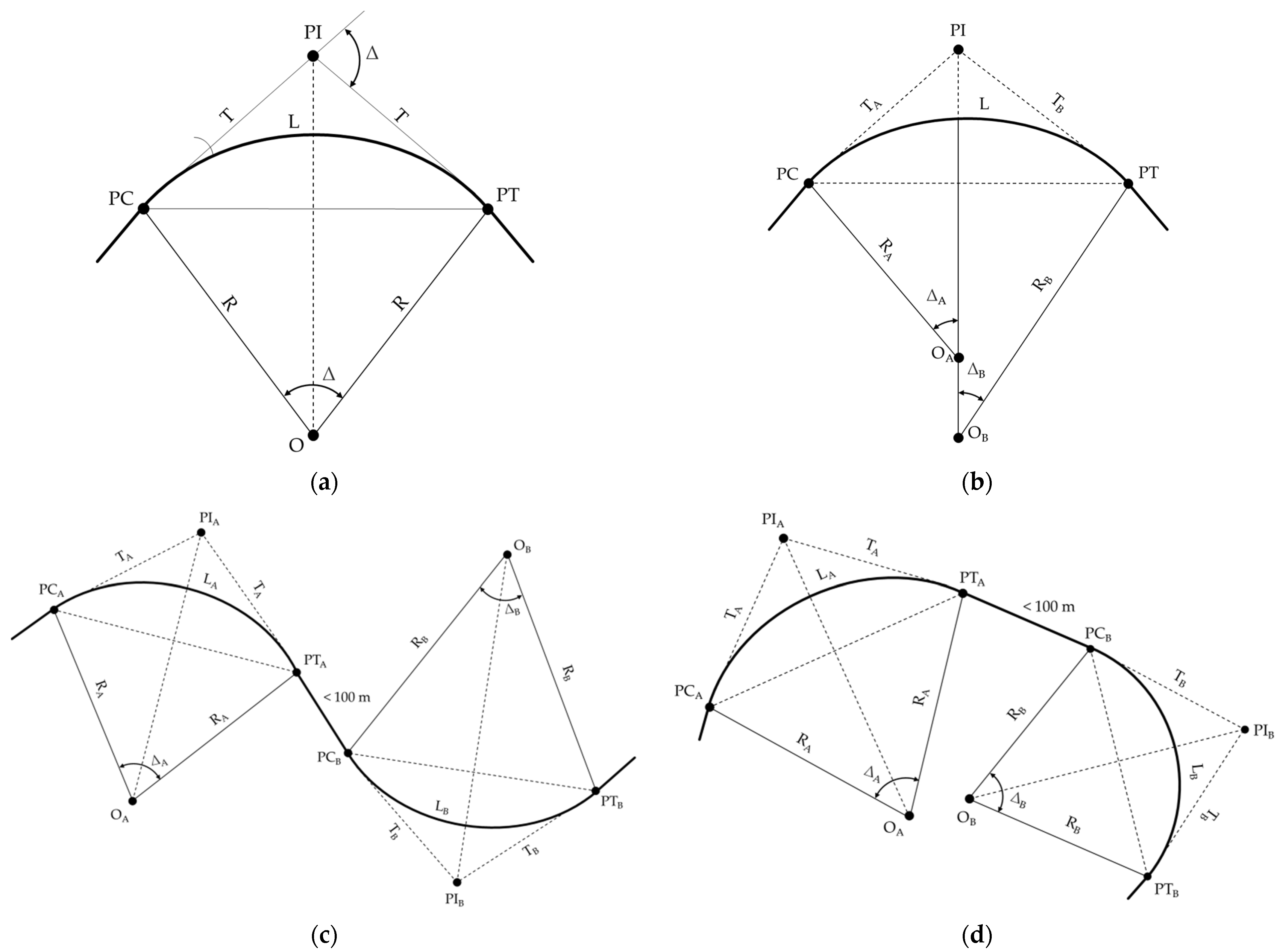
In general, there are four types of horizontal curve segments: a circular curve, a compound curve, a reverse curve, and a broken-back curve. The layout of each curve type is illustrated in Figure 1.

3.1.1. Circular Curve

A circular curve is the most common type of horizontal curve. It consists of a single arc of a uniform radius (R), which connects two intersecting tangents at a point of intersection (PI) with a deflection angle (∆). The curve links two straight road segments at a point of curvature (PC) and a point of tangent (PT).

3.1.2. Compound Curve

A compound curve is a curve that consists of a series of two or more simple arcs of different radius (R_A and R_B) bending in the same direction and laying on the same side of their common tangent. Compound curves may cause operational problems since drivers may not perceive the change in curvature and may not anticipate a change in side-friction demand [9,29]. Normally, for a compound curve, the radius of the larger curve is more than 1.5 times that of the smaller curve [33].

3.1.3. Reverse Curve

A reverse curve is the arrangement of two consecutive circular curves with a short length of less than 100 m tangent between the curves which bend in the opposite direction [9,29]. Even though a reverse curve is suitable for tracks lying in a mountainous or rural region, this geometry should be avoided.

3.1.4. Broken-Back Curve

A broken-back curve is the arrangement of two consecutive circular curves with a short length of less than 100 m tangent connecting two arcs that have centres on the same side. Broken-back curves should be avoided, if possible, except where unusual topographical or right-of-way conditions make other alternatives impractical, as most drivers do not expect successive curves to be in the same direction [9].

3.2. Predictive Method

The predictive method is used to estimate the expected annual average crash frequency of an individual road segment. The model, which is a function of traffic volume and roadway geometries over a roadway network, provides a statistical relationship between the expected number of crashes and roadway characteristics [34,35,36]. The estimate relies upon models developed from observed crash data for several similar sites [22].

Safety Performance Functions (SPFs) are statistical-based crash prediction models which are used as tools to quantitatively measure the safety performance of a roadway in terms of the average crash frequency for a facility type with specific base conditions. The estimation can be made for existing conditions, alternative conditions, or proposed new roadways. This predictive method is applied to a given period, traffic volume, and constant geometric design characteristics of the roadway with critical safety concerns [22].

Relationships among traffic volume, constant geometric design characteristics of the roadway, and the average crash frequency can be modelled by many functional forms of Safety Performance Functions (SPFs). The most common functional forms are Poisson and Negative Binomial Safety Performance Function [36]. Moreover, Part C of the Highway Safety Manual (HSM) [22] provides a structured methodology for estimating the expected average crash frequency of a site, facility, or roadway network over a given period, the geometric design, traffic control features, and traffic volume.

3.2.1. Poisson Safety Performance Function

The Poisson safety performance function or Poisson regression model, based on the Poisson probability distribution, is the fundamental method used for modelling count response data [37]. The Poisson regression model assumes that the observed outcome variable follows Poisson distribution and is characterized by a mean expected value which is also its variance [38]. A standard expression for the Poisson regression model is:

$$\mathrm{f}(\mathrm{y};\mathrm{p},\mathrm{n})=\left(\begin{array}{l}{\mathrm{n}}_{\mathrm{i}}\\ {\mathrm{y}}_{\mathrm{i}}\end{array}\right){\mathrm{p}}_{\mathrm{i}}{}^{{\mathrm{y}}_{\mathrm{i}}}{(1-{\mathrm{p}}_{\mathrm{i}})}^{{\mathrm{n}}_{\mathrm{i}}-{\mathrm{y}}_{\mathrm{i}}}$$

(1)

where f is the probability function of “n choose y”, with y indicating the number of Bernoulli successes, n is the number of trials, and p is the probability of success. When the binomial mean ($\lambda$) is the product of the number of trials (n) and the probability of success (p). Letting n become very large, and p become very small, we can reformulate the binomial distribution as:

$$\mathrm{f}(\mathrm{y};\lambda )=\frac{{\lambda }_{\mathrm{i}}{}^{{\mathrm{y}}_{\mathrm{i}}}{\mathrm{e}}^{-{\lambda }_{\mathrm{i}}}}{{\mathrm{y}}_{\mathrm{i}}!}$$

(2)

To predict the crash frequency. The linear function of the Poisson safety performance function takes on the form as follows:

$$\mathrm{N}=\mathrm{e}\mathrm{x}\mathrm{p}({\mathrm{B}}_0+{\mathrm{B}}_1{\mathrm{x}}_1+{\mathrm{B}}_2{\mathrm{x}}_2+\dots +{\mathrm{B}}_{\mathrm{n}}{\mathrm{x}}_{\mathrm{n}})$$

(3)

where N is the number of predicted crashes (crashes per year), x_i is an independent variable, B₀ is a function intercept, B_i is a coefficient for its associated variable x_i, and i = {1, 2, …, n} where n is the number of independent variables.

3.2.2. Negative Binomial Safety Performance Function

Another functional form of safety performance function is developed using the negative binomial distribution, which is an extension of the Poisson distribution [39] known as the Poisson-Gamma distribution. The negative binomial distribution is more commonly used to model crash data than the Poisson distribution because the variance typically exceeds the mean. Data for which the variance exceeds the mean are said to be over-dispersed, and the negative binomial distribution is very well suited to modelling over-dispersed data [22]. A standard expression for the negative binomial regression model is:

$$\mathrm{f}(\mathrm{y};\mathrm{p},\mathrm{r})=\left(\begin{array}{c}{\mathrm{y}}_{\mathrm{i}}+\mathrm{r}-1\\ \mathrm{r}-1\end{array}\right){\mathrm{p}}_{\mathrm{i}}{}^{\mathrm{r}}{(1-{\mathrm{p}}_{\mathrm{i}})}^{{\mathrm{y}}_{\mathrm{i}}}$$

(4)

where f is the probability function, p is the probability of success, and consider y as the number of failures before the r-th success. Consider the situation when the r-th success is on the x-th trial. It follows then that the previous r − 1 successes can occur at any time in the previous x − 1 trials [37]. We can reformulate the binomial distribution as:

$$\mathrm{f}(\mathrm{y};\mathrm{p},\mathrm{r})=\frac{\left({\mathrm{y}}_{\mathrm{i}}+\mathrm{r}-1\right)!}{{\mathrm{y}}_{\mathrm{i}}!(\mathrm{r}-1)!}{\mathrm{p}}_{\mathrm{i}}{}^{\mathrm{r}}{(1-{\mathrm{p}}_{\mathrm{i}})}^{{\mathrm{y}}_{\mathrm{i}}}$$

(5)

To predict the crash frequency, the linear function of the negative binomial safety performance function also takes on the following form as:

$$\mathrm{N}=\mathrm{e}\mathrm{x}\mathrm{p}({\mathrm{B}}_0+{\mathrm{B}}_1{\mathrm{x}}_1+{\mathrm{B}}_2{\mathrm{x}}_2+\dots +{\mathrm{B}}_{\mathrm{n}}{\mathrm{x}}_{\mathrm{n}})$$

(6)

where N is the number of predicted crashes (crashes per year), x_i is an independent variable, B₀ is a function intercept, B_i is a coefficient for its associated variable x_i, and i = {1, 2, …, n} where n is the number of independent variables.

3.2.3. Calibrated Highway Safety Manual Safety Performance Function

Highway Safety Manual (HSM) Safety Performance Functions (SPFs) are developed through statistical regression modelling based on the negative binomial distribution, which is better suited to modelling the high natural variability of crash data than traditional modelling techniques. To apply the HSM safety performance functions for any site type with specific base conditions, the functions are calibrated to estimate the average crash frequency by accounting for the local factors that affect the safety of a roadway to fit local conditions for use in evaluating safety performance [36,40].

In the HSM, the Safety Performance Function (SPF) for roadway segments on two-lane rural roads under base conditions is presented as a function of annual average daily traffic and roadway segment length converting to the metric unit as follows:

$${\mathrm{N}}_{\mathrm{s}\mathrm{p}\mathrm{f}}=6.21\times \mathrm{A}\mathrm{A}\mathrm{D}\mathrm{T}\times \mathrm{L}\times 365\times {10}^{-6}\times {\mathrm{e}}^{-0.312}$$

(7)

where N_spf is the number of predicted crashes by safety performance function under base condition (crashes per year), AADT is annual average daily traffic (vehicles per day), and L is roadway segment length (m).

The SPF requires adjustment to consider the difference between base conditions, specific site conditions, and local conditions [22]. Crash modification factors (CMFs) and calibration factor (C_x) are used as a multiplier applying to the SPF to obtain the predicted crashes (N_predicted) as follows:

$${\mathrm{N}}_{\mathrm{p}\mathrm{r}\mathrm{e}\mathrm{d}\mathrm{i}\mathrm{c}\mathrm{t}\mathrm{e}\mathrm{d}}=(6.21\times \mathrm{A}\mathrm{A}\mathrm{D}\mathrm{T}\times \mathrm{L}\times 365\times {10}^{-6}\times {\mathrm{e}}^{-0.312})\times {\mathrm{C}}_{\mathrm{x}}\times \mathrm{C}\mathrm{M}\mathrm{F}$$

(8)

Crash modification factors (CMFs) are used to account for the differences between the base condition and the site conditions specific to the specified road features. Under the base conditions, the value of a CMF is 1.00. In comparison to the base condition, CMF values indicate whether the specified road feature reduces (if CMF is less than 1.00) or increases (if CMF is greater than 1.00) the estimated crash frequency.

A calibration factor (C_x), which allows the SPF to keep its original model form by applying a multiplicative factor to the aggregate number of predicted crashes is equal to the aggregate number of observed crashes [40], is used to account for the differences between the base condition and the local conditions. It is the ratio of the total number of observed crashes (N_observed) and predicted crashes (N_predicted) as follows:

$${\mathrm{C}}_{\mathrm{x}}=\frac{{\displaystyle \sum {\mathrm{N}}_{\mathrm{o}\mathrm{b}\mathrm{s}\mathrm{e}\mathrm{r}\mathrm{v}\mathrm{e}\mathrm{d}}}}{{\displaystyle \sum {\mathrm{N}}_{\mathrm{p}\mathrm{r}\mathrm{e}\mathrm{d}\mathrm{i}\mathrm{c}\mathrm{t}\mathrm{e}\mathrm{d}}}}$$

(9)

3.3. Model Accuracy

To measure the average magnitude of the errors in predictions, there are two metrics commonly used to compare the accuracy of prediction models including mean absolute error (MAE) and root mean square error (RMSE) [13,18,41,42].

3.3.1. Mean Absolute Error

Mean Absolute Error (MAE) is the average absolute difference between the predicted crash frequency and the observed crash frequency expressing the same phenomenon, given by the following formula:

$$\mathrm{M}\mathrm{A}\mathrm{E}=\frac{{\displaystyle \sum _{\mathrm{i}=1}^{\mathrm{n}}|\widehat{{\mathrm{y}}_{\mathrm{i}}}-{\mathrm{y}}_{\mathrm{i}}|}}{\mathrm{n}}$$

(10)

where $\widehat{{\mathrm{y}}_{\mathrm{i}}}$ is the predicted crash frequency for observation i, ${\mathrm{y}}_{\mathrm{i}}$ is the observed crash frequency for observation i, and n is the total number of observations.

3.3.2. Root Mean Square Error

Root Mean Square Error (RMSE) is the standard deviation of the prediction errors that are the difference between the predicted crash frequency and the observed crash frequency, given by the following formula:

$$\mathrm{R}\mathrm{M}\mathrm{S}\mathrm{E}=\sqrt{\frac{1}{\mathrm{n}}\times {\displaystyle \sum {(\widehat{{\mathrm{y}}_{\mathrm{i}}}-{\mathrm{y}}_{\mathrm{i}})}^2}}$$

(11)

where $\widehat{{\mathrm{y}}_{\mathrm{i}}}$ is the predicted crash frequency for observation i, ${\mathrm{y}}_{\mathrm{i}}$ is the observed crash frequency for observation i, and n is the total number of observations.

4. Data Collection

In Thailand, rural road alignments were designed and built upon limited right-of-way, land acquisition, and financial resources leading to mediocre efficiency and safety. Seeking to improve roadway safety, Thailand’s Department of Rural Roads (DRR) is collecting roadway-specific data for the database to thoroughly comprehend how the roadway geometry and characteristics impact the crash frequency. As technological advancement enables easier transportation data collection, more roadway attributes can be measured and recorded in the DRR database.

This study was based on data from over 47,000-kilometer rural road network, which accounts for 10 percent of the road network across the nation. Relevant data on two-lane rural roads were employed including road alignment data, road attribute data, and historical crash data.

4.1. Road Alignment Data

The alignment data of two-lane rural roads in Thailand were collected from a Global Positioning System (GPS) vehicle tracking technology. The system combines the use of automatic vehicle location in individual vehicles with software that tracks the vehicle location including longitude and latitude coordinates once a meter. The raw data of geographic coordinates were analysed to identify straight and curve road segments. For each horizontal curve segment, the type of curve was classified as a circular curve, a compound curve, a reverse curve, and a broken-back curve. In addition, the radius (R), the point of curvature (PC), the point of intersection (PI), the point of tangent (PT), and the length (L) associated with each curve segment were determined.

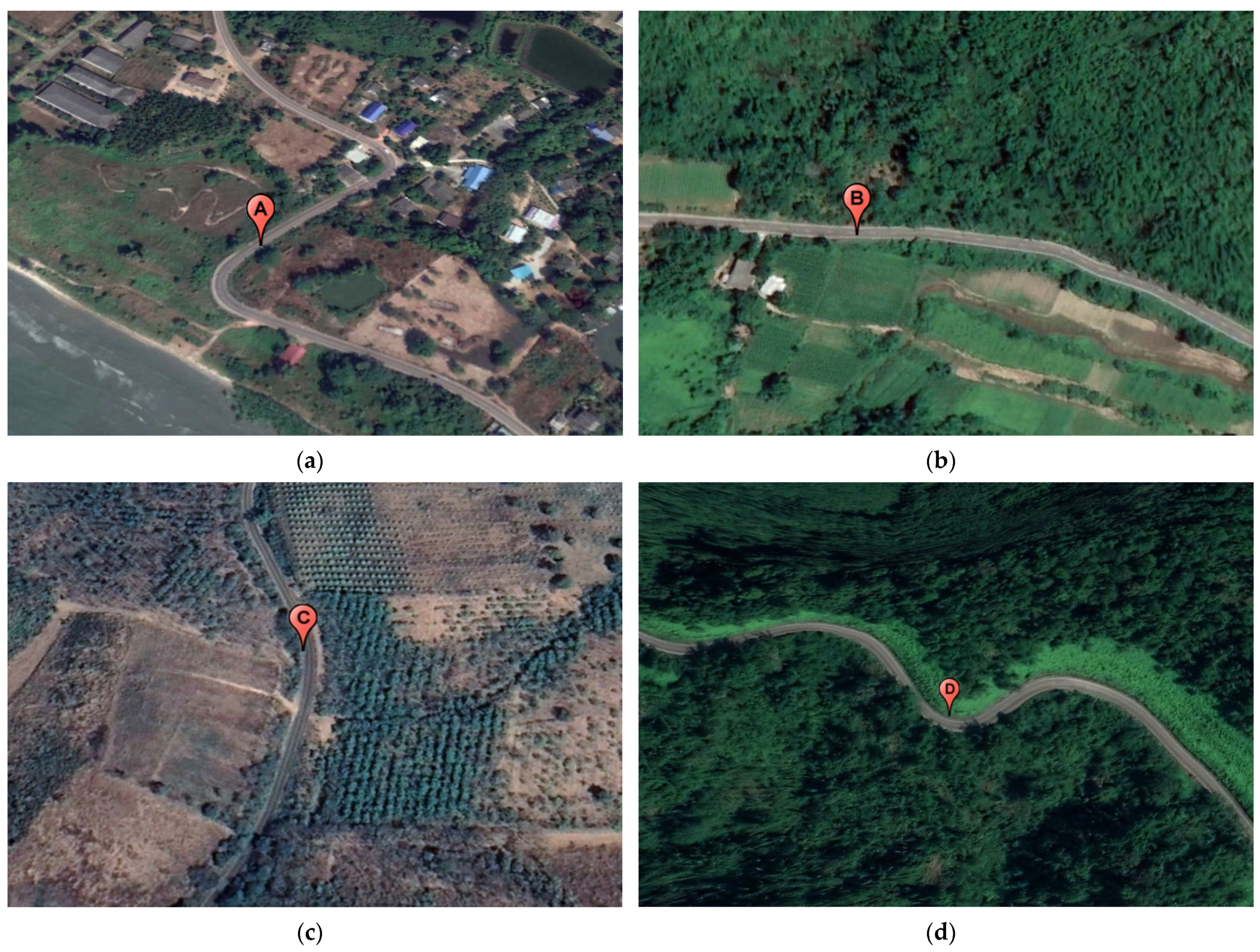
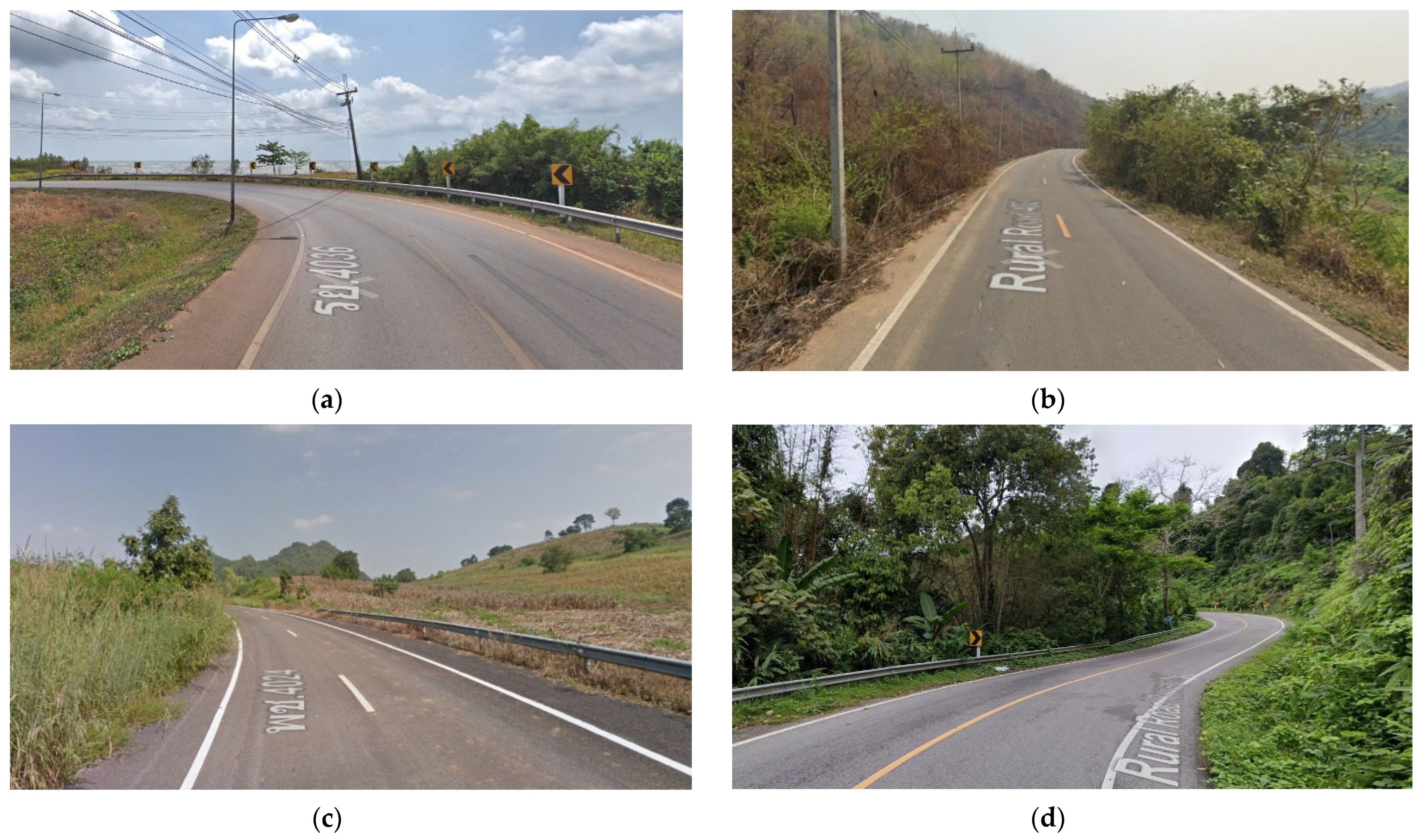
With GPS tracking technology, a total of 86,862 horizontal curve segments on the rural road network in Thailand can be identified. They are classified into four types according to their roadway geometry. Among 86,862 curves, there are 50,030 circular curves, 6138 compound curves, 20,697 reverse curves, and 9827 broken-back curves. Examples of horizontal curve segments on two-lane rural roads in Thailand by curve types are shown as top views in Figure 2 and as street views in Figure 3.

4.2. Road Attribute and Traffic Data

As mentioned previously, this study aims to study the relationship among road geometric condition, traffic condition, and crash frequency and identify the most significant parameters affecting crash frequency. The data on both road geometric conditions and traffic conditions used in this study are classified into two categories: (1) road geometric and roadway characteristics gathered from the rural road asset database such as lane width, shoulder width, shoulder type, centreline and edge-lines, pavement condition, signs, guideposts, and lateral obstructions; and (2) traffic data gathered from the traffic rural road database.

4.3. Historical Crash Data

The historical crash data associated with each horizontal curve segment on two-lane rural roads from 2016 to 2018 were collected from the crash database. In the period, there were 291 crashes in total: 167 crashes on circular curves, 22 crashes on compound curves, 67 crashes on reverse curves, and 35 crashes on broken-back curves.

Table 1. The 3-year crash rate and casualty rate by types of curves.

Curve Type	Number of Curves	Number of Crashes	Crash Rate (Per 100 Curves)	Number of Casualties	Casualty Rate (Per 100 Curves)
Circular Curve	50,030	167 (57.29%)	0.334	77	0.154
Compound Curve	6138	22 (7.56%)	0.358	14	0.228
Reverse Curve	20,697	67 (23.02%)	0.324	56	0.271
Broken-back Curve	9827	35 (12.03%)	0.356	17	0.173
Total	86,862	291		164

presents the result from preliminary statistical analysis of the 3-year historical crash and casualty data on the period. To identify the risk of crash occurrence associated with each type of horizontal curve, the crash and casualty rates per 100 curves were presented. In terms of crash rate per 100 curves, the highest is on compound curves (0.358) followed by broken-back curves, circular curves, and reverse curves, respectively. However, in terms of casualty rate per 100 curves, the highest is on reverse curves (0.271) followed by compound curves, broken-back curves, and circular curves, respectively. Hence, the types of curves would affect crash occurrence and severity on horizontal alignments.

5. Data Analysis and Results

This section is divided into four sections as descriptive statistics, correlation of variables, development of safety performance functions, and goodness of measures and model accuracy.

5.1. Descriptive Statistics

In this study, a total of 86,599 horizontal curve segments on a two-lane rural road network in Thailand was used to analyse crash prediction models. It is noted that 263 curve segments were excluded before analysis to handle missing data, the method called list-wise deletion [42].

Data used in the analysis consist of (1) road alignment data including curve length, curve radius, types of curves; (2) road attributes including lane width and shoulder width and traffic data in terms of annual average daily traffic (AADT); and (3) the historical crash data from 2016 to 2018 on each two-lane horizontal curve segment on rural road networks as details in the previous section.

The descriptive statistics for the dependent and independent variables of the prediction models collected from the 86,599 horizontal curve segments on two-lane rural roads are shown in

Table 2. Summary descriptive statistics for horizontal curve segments.

Variable	Min	Max	Mean	Std. Dev.
Dependent Variable
Observed Crashes (per 3 years)	0.00	7.00	0.015	0.143
Independent Variables
Annual Average Daily Traffic (vehicles/day)	4.00	32,890.00	2087.7	2195.2
Natural log of Annual Average Daily Traffic (vehicles/day)	1.39	10.40	7.280	0.886
Segment Length (m)	150.00	1306.00	177.24	32.04
Natural log of Segment Length (m)	5.01	7.17	5.165	0.150
Horizontal Curve Radius (m)	8.90	1098.29	211.05	162.37
Lane Width (m)	2.00	3.50	2.980	0.196
Shoulder Width (m)	0.00	5.00	1.002	0.849
Type: Compound Curve (1 if present, 0 otherwise)	0.00	1.00	0.071	0.256
Type: Reverse Curve (1 if present, 0 otherwise)	0.00	1.00	0.113	0.317
Type: Broken-Back Curve (1 if present, 0 otherwise)	0.00	1.00	0.239	0.426

.

5.2. Correlation of Variables

To test the correlation of variables, the Pearson chi-square test is commonly used. This technique is suitable for correlation analysis between two categorical variables. The variables were tested for multicollinearity by computing the Pearson correlation coefficients. In general, correlation coefficients can range in value from −1.00 to +1.00 where a value of −1.00 represents a perfect negative correlation while a value of +1.00 represents a perfect positive relationship [43]. However, the variables with high correlation coefficients (p-value greater than 0.05) were eliminated from the models because one variable is dependent upon another.

Crash frequency was determined as the dependent variable of the crash prediction model, the correlation between dependent and independent variables are shown in

Table 3. Correlation between dependent and independent variables.

Independent Variable	Label	Pearson Correlation	p-Value
Natural log of Annual Average Daily Traffic	ln(AADT)	0.076	0.000 *
Natural log of Segment Length	ln(L)	0.028	0.000 *
Horizontal Curve Radius	R	0.002	0.000 *
Lane Width	Lw	0.026	0.000 *
Shoulder Width	Sw	0.020	0.000 *
Type: Compound Curve	CC	−0.001	0.846
Type: Reverse Curve	RC	−0.004	0.294
Type: Broken-Back Curve	BC	−0.008	0.022 *

* Correlation is significant at the 0.05 level (2-tailed).

. As can be seen, annual average daily traffic (AADT), curve segment length, curve radius, lane width, and shoulder-width indicated their increasing effect on crash frequency due to the significant positive correlation whereas the presence of broken-back curve indicated its decreasing effect on crash frequency due to the significant negative correlation. For the presence of both compound curve and reverse curve, there is relatively no effect on crash frequency.

To consider the risk of crash occurrence associated with each type of horizontal curve, the study compared the results based on the correlation of variables with the results from preliminary statistical analysis of crash and casualty data from the previous section. There is a conflict, only the broken-back curve is the type of curve affecting the occurrence of crashes.

To consider the correlation between each independent variable, the details are shown in

Table 4. Correlation between independent variables.

Variable	Pearson Correlation (p-Value)
	CC	BC	RC	R	ln(AADT)	ln(Lc)	Lw	Sw
CC	1	−0.099 *	−0.154 *	−0.045 *	−0.024 *	0.004	−0.023 *	−0.017 *
	-	(0.000)	(0.000)	(0.000)	(0.000)	(0.212)	(0.000)	(0.000)
BC	−0.099 *	1	−0.200 *	−0.008 *	−0.030 *	−0.014 *	−0.035 *	−0.043 *
	(0.000)	-	(0.000)	(0.015)	(0.000)	(0.000)	(0.000)	(0.000)
RC	−0.154 *	−0.200 *	1	−0.150 *	−0.056 *	−0.037 *	−0.056 *	−0.070 *
	(0.000)	(0.000)	-	(0.000)	(0.000)	(0.000)	(0.000)	(0.000)
R	−0.045 *	−0.008 *	−0.150 *	1	0.094 *	0.235 *	0.066 *	0.086 *
	(0.000)	(0.015)	(0.000)	-	(0.000)	(0.000)	(0.000)	(0.000)
ln(AADT)	−0.024 *	−0.030 *	−0.056 *	0.094 *	1	0.025 *	0.132 *	0.183 *
	(0.000)	(0.000)	(0.000)	(0.000)	-	(0.000)	(0.000)	(0.000)
ln(Lc)	0.004	−0.014 *	−0.037 *	0.235 *	0.025 *	1	0.025 *	0.019 *
	(0.212)	(0.000)	(0.000)	(0.000)	(0.000)	-	(0.000)	(0.000)
Lw	−0.023 *	−0.035 *	−0.056 *	0.066 *	0.132 *	0.025 *	1	0.294 *
	(0.000)	(0.000)	(0.000)	(0.000)	(0.000)	(0.000)	-	(0.000)
Sw	−0.017 *	−0.043 *	−0.070 *	0.086 *	0.183 *	0.019 *	0.294 *	1
	(0.000)	(0.000)	(0.000)	(0.000)	(0.000)	(0.000)	(0.000)	-

* Correlation is significant at the 0.05 level (2-tailed).

.

5.3. Development of Safety Performance Functions

The focus on safety performance functions (SPFs) of this paper is two-fold. First, this study was designed to develop two functional forms of safety performance function for horizontal curve segment on two-lane rural roads in Thailand including Poisson safety performance functions and negative binomial safety performance functions. Another focus is to compare the two safety performance functions to the calibrated safety performance function using Highway Safety Manual procedures.

5.3.1. Poisson Safety Performance Function

To develop a Poisson safety performance function in this study using 86,599 datasets, the significant independent variables were included in the model following a backward stepwise variable selection procedure. It begins with a full model and, at each step, gradually eliminates variables from the regression model to find a reduced model that best explains the data [44].

The safety performance function based on the Poisson distribution for two-lane rural horizontal curve segments is presented as follows (statistical details are shown in

Table 5. Parameter Estimates of Poisson safety performance function.

Parameter	B	Std. Error	95% Wald Confidence Interval		Hypothesis Test
			Lower	Upper	Wald Chi-Square	df	Sig.
(Intercept)	−20.423	0.9095	−22.205	−18.640	504.163	1	0.000
R	−0.001	0.0002	−0.001	0.000	13.306	1	0.000
ln(AADT)	0.853	0.0326	0.789	0.916	682.345	1	0.000
ln(L)	1.419	0.1511	1.123	1.716	88.197	1	0.000
Lw	0.850	0.1484	0.559	1.141	32.769	1	0.000

):

$$\mathrm{N}=\mathrm{e}\mathrm{x}\mathrm{p}(-20.423+0.853\mathrm{l}\mathrm{n}(\mathrm{A}\mathrm{A}\mathrm{D}\mathrm{T})+1.419\mathrm{l}\mathrm{n}(\mathrm{L})-0.001\mathrm{R}+0.850\mathrm{L}\mathrm{w})$$

(12)

where N is the number of predicted crashes, ln(AADT) is the natural log of annual average daily traffic (vehicles/day), ln(L) is the natural log of roadway segment length (m), R is horizontal curve radius (m), and Lw is lane width (m).

5.3.2. Negative Binomial Safety Performance Function

A negative binomial safety performance function in this study using 86,599 datasets was developed using the same variable selection procedure as explained in the Poisson safety performance function. The safety performance function based on the negative binomial distribution for two-lane rural horizontal curve segments is presented as follows (statistical details are shown in

Table 6. Parameter Estimates of the negative binomial safety performance function.

Parameter	B	Std. Error	95% Wald Confidence Interval		Hypothesis Test
			Lower	Upper	Wald Chi-Square	df	Sig.
(Intercept)	−20.287	0.9317	−22.113	−18.461	474.076	1	0.000
R	−0.001	0.0002	−0.001	0.000	12.989	1	0.000
ln(AADT)	0.849	0.0334	0.783	0.914	646.648	1	0.000
ln(L)	1.424	0.1554	1.119	1.728	83.935	1	0.000
Lw	0.807	0.1510	0.511	1.103	28.576	1	0.000

):

$$\mathrm{N}=\mathrm{e}\mathrm{x}\mathrm{p}(-20.287+0.849\mathrm{l}\mathrm{n}(\mathrm{A}\mathrm{A}\mathrm{D}\mathrm{T})+1.424\mathrm{l}\mathrm{n}(\mathrm{L})-0.001\mathrm{R}+0.807\mathrm{L}\mathrm{w})$$

(13)

where N is the number of predicted crashes, ln(AADT) is the natural log of annual average daily traffic (vehicles/day), ln(L) is the natural log of roadway segment length (m), R is horizontal curve radius (m), and Lw is lane width (m).

5.3.3. Calibrated Highway Safety Manual Safety Performance Function

The general level of predicted crash frequency using the Highway Safety Manual (HSM) safety performance function may vary substantially from one jurisdiction to another for a variety of reasons [22]. To develop the safety performance function for horizontal curve segments of two-lane rural roads in Thailand using Highway Safety Manual procedure, it is necessary to calibrate the function to local state or geographic conditions using crash modification factors (CMFs) and calibration factor (C_x) as a multiplier applying to the safety performance function as the following form:

$$\mathrm{N}=(6.21\times \mathrm{A}\mathrm{A}\mathrm{D}\mathrm{T}\times \mathrm{L}\times 365\times {10}^{-6}\times {\mathrm{e}}^{-0.312})\times {\mathrm{C}}_{\mathrm{x}}\times \mathrm{C}\mathrm{M}\mathrm{F}$$

(14)

where N is the number of predicted crashes, AADT is the annual average daily traffic (vehicles/day), L is roadway segment length (m).

In this study, crash modification factors (CMFs), which are used to adjust the SPF for rural two-lane roadway segments to account for differences between the base conditions and the local site conditions, are the following multiplier:

$$\mathrm{C}\mathrm{M}\mathrm{F}=\mathrm{C}\mathrm{M}{\mathrm{F}}_{1\mathrm{r}}\times \mathrm{C}\mathrm{M}{\mathrm{F}}_{2\mathrm{r}}\times \mathrm{C}\mathrm{M}{\mathrm{F}}_{3\mathrm{r}}$$

(15)

where CMF_1r is the crash modification factor for the effect of lane width on total crashes, CMF_2r is the crash modification factor for shoulder width and type, and CMF_3r is the crash modification factor for horizontal curves (length, radius, and presence or absence of spiral transitions). The details of each crash modification factor are as follows:

• Crash modification factor for lane width (CMF_1r)

The crash modification factor for lane width on two-lane roadway segments was developed from the work of Zegeer et al. [45] and Griffin and Mak [46] expressed on this basis are adjusted to total crashes within the predictive method using the following equation [22]:

$$\mathrm{C}\mathrm{M}{\mathrm{F}}_{1\mathrm{r}}=(\mathrm{C}\mathrm{M}{\mathrm{F}}_{\mathrm{r}\mathrm{a}}-1.0)\times {\mathrm{p}}_{\mathrm{r}\mathrm{a}}+1.0$$

(16)

where CMF_1r is the crash modification factor for lane width, CMF_ra is the crash modification factor for the effect of lane width on related crashes (

Table 7. Crash modification factor for lane width on roadway segments.

Lane Width (m)	AADT (Vehicles per Day)
	<400	400 to 2000	>2000
2.74 or less	1.05	$1.05+2.81\times {10}^{-4}(\mathrm{A}\mathrm{A}\mathrm{D}\mathrm{T}-400)$	1.50
3.05	1.02	$1.02+1.75\times {10}^{-4}(\mathrm{A}\mathrm{A}\mathrm{D}\mathrm{T}-400)$	1.30
3.35	1.01	$1.01+2.50\times {10}^{-5}(\mathrm{A}\mathrm{A}\mathrm{D}\mathrm{T}-400)$	1.05
3.66 or more	1.00	1.00	1.00

Note: A CMF value can be interpolated using either of these exhibits [26].

), and p_ra is the proportion of total crashes constituted by related crashes.

• Crash modification factor for shoulder width and type ($\mathrm{C}\mathrm{M}{\mathrm{F}}_{2\mathrm{r}}$)

The crash modification factor for shoulder width and shoulder type are based on the results of Zegeer et al. [47] expressed on this basis are adjusted to total crashes within the predictive method using the following equation [22]:

$$\mathrm{C}\mathrm{M}{\mathrm{F}}_{2\mathrm{r}}=(\mathrm{C}\mathrm{M}{\mathrm{F}}_{\mathrm{w}\mathrm{r}\mathrm{a}}\times \mathrm{C}\mathrm{M}{\mathrm{F}}_{\mathrm{t}\mathrm{r}\mathrm{a}}-1.0)\times {\mathrm{p}}_{\mathrm{r}\mathrm{a}}+1.0$$

(17)

where CMF_2r is the crash modification factor for the effect of shoulder width and shoulder type on total crashes, CMF_wra is the crash modification factor for related crashes based on shoulder width (

Table 8. Crash modification factor for shoulder width on roadway segments.

Lane Width (m)	AADT (Vehicles per Day)
	<400	400 to 2000	>2000
0	1.10	$1.10+2.5\times {10}^{-4}(\mathrm{A}\mathrm{A}\mathrm{D}\mathrm{T}-400)$	1.50
0.61	1.07	$1.07+1.43\times {10}^{-4}(\mathrm{A}\mathrm{A}\mathrm{D}\mathrm{T}-400)$	1.30
1.22	1.02	$1.02+8.125\times {10}^{-5}(\mathrm{A}\mathrm{A}\mathrm{D}\mathrm{T}-400)$	1.15
1.83	1.00	1.00	1.00
2.44 or more	0.98	$0.98-6.875\times {10}^{-5}(\mathrm{A}\mathrm{A}\mathrm{D}\mathrm{T}-400)$	0.87

Note: A CMF value can be interpolated using either of these exhibits [22].

), CMF_tra is the crash modification factor for related crashes based on shoulder type (

Table 9. Crash modification factor for shoulder type on roadway segments.

Shoulder Type	Shoulder Width (m)
	0	0.30	0.61	0.91	1.22	1.83	2.44
Paved	1.00	1.00	1.00	1.00	1.00	1.00	1.00
Gravel	1.00	1.00	1.01	1.01	1.01	1.02	1.02
Composite	1.00	1.01	1.02	1.02	1.03	1.04	1.06
Turf	1.00	1.01	1.03	1.04	1.05	1.08	1.11

), and p_ra is the proportion of total crashes constituted by related crashes.

• Crash modification factor for horizontal curves (CMF_3r)

The crash modification factor for horizontal curves: length, radius, and presence or absence of spiral transitions has been determined from the regression model developed by Zegeer et al. [48]. The CMF for horizontal curvature is in the form of an equation and yields a factor. Given the curve length, curve radius, and the presence of spiral transitions on horizontal curves, CMF is determined using the following equation [22]:

$$\mathrm{C}\mathrm{M}{\mathrm{F}}_{3\mathrm{r}}=\frac{(1.55\times 0.000621\times {\mathrm{L}}_{\mathrm{c}})+\left(\frac{80.2}{3.28\times \mathrm{R}}\right)-(0.012\times \mathrm{S})}{(1.55\times 0.000621\times {\mathrm{L}}_{\mathrm{c}})}$$

(18)

where CMF_3r is the crash modification factor for the effect of horizontal alignment on total crashes, L_c is the length of a horizontal curve (m), R is the radius of curvature (m), and S equals 1 if the spiral transition curve is present; equals 0 if not present; equals 0.5 if a spiral transition curve is present at one end of the horizontal curve.

To adjust the adopted safety performance function to local conditions, the calibration factor was accomplished developing by a selected number of sites and being done in the same period of time. The highway safety manual calibration procedure suggests that at least 30 to 50 sites with at least 100 crashes per year should be included for each facility for this calibration analysis. To avoid a site selection bias, the sites should be randomly selected and then the number of crashes should be determined [22].

The recommendation by the Highway Safety Manual does not apply to this study because the target number of crashes of 100 per year still could not be achieved. Referring to the work of Xie et al. [49], the target number of crashes can be modified to that value based on the average crash history for the facility type. Therefore, at least 30 to 50 sites with at least 50 crashes every three years for each facility were used for this calibration analysis of this study.

The result of the calibration analysis classified by types of curves is shown in

Table 10. Calibration factor classified by types of curves.

Types of Curves	Observed Crashes	Predicted Crashes	Calibration Factor
Simple Curve	66	111.90	0.570
Compound Curve	50	127.58	0.392
Reverse Curve	50	83.75	0.597
Broken-back Curve	50	106.46	0.470

. The calibration factor is 0.570 for simple curve, 0.392 for compound curve, 0.597 for reverse curve, and 0.470 for the broken-back curve.

5.4. Goodness of Measures and Model Accuracy

Comparing the goodness-of-fit among the estimation models, the most significant parameters affecting crash frequency on two-lane horizontal curve segments is lane width, followed by curve length, daily traffic volume, and curve radius, respectively. Elasticity analysis was used to examine the marginal effects of the variables on crash frequency.

• a percent increase in lane width causes an increase of 2.582% in crashes.
• a percent increase in curve length causes an increase of 1.422% in crashes.
• a percent increase in daily traffic causes an increase of 0.852% in crashes.
• a percent increase in curve radius causes a decrease of 0.797% in crashes.

To compare the accuracy among prediction models, two metrics including mean absolute error (MAE) and root mean square error (RMSE) were used. A summary of the comparison is presented in

Table 11. The comparison of model accuracy.

Metric	Safety Performance Functions
	Poisson	Negative Binomial	Calibrated HSM
Mean Absolute Error (MAE)	0.726	0.727	0.528
Root Mean Square Error (RMSE)	0.770	0.771	0.657

. Based on the prediction performance, the calibrated Highway Safety Manual safety performance function is found to be the most effective in predicting the number of crashes on horizontal curve segments on two-lane rural roads followed by negative binomial and Poisson safety performance functions.

6. Conclusions

On two-lane rural roads in Thailand, the number of road crashes continues to rise significantly. Curve segments are among the most hazardous locations which lead to road crashes and economic losses, which are totally unacceptable. There is an urgent need to understand the mechanism of crash risk on two-lane rural curve segments, and to identify the relationship between crash frequency and roadway characteristics of each horizontal curve.

This study aims to develop Safety Performance Functions (SPFs) using Generalised Linear Model (GLM) techniques as a crash prediction model to identify the relationship among road geometric conditions, traffic conditions, and crash frequency, and to determine the most significant parameters affecting crash frequency. The datasets used in this study were collected from road data inventories of the rural road network which are systematically measured and recorded using advanced technologies including (1) 3-year historical crash data from crash reports, (2) the alignment data of horizontal curve segments collected from a GPS vehicle tracking technology, and (3) the road attribute and traffic data of each horizontal curve segment from rural road asset databases.

With the aim of the identification, this study compared three functional forms of SPFs for horizontal curve segments of two-lane rural roads including the Poisson regression model, negative binomial regression model, and calibrated HSM model. The dataset of 86,599 horizontal curve segments was used in this study. They are (1) road alignment data, e.g., curve segment length, horizontal curve radius, and types of curves; (2) roadway geometric design elements and characteristics, e.g., lane width, shoulder width, and (3) crash data from 2016 to 2018 on curve segments.

For the Poisson and Binomial Negative safety performance functions, the significant parameters affecting crash frequency include lane width, curve segment length, traffic volumes, curve radius, and types of horizontal curves. For the calibrated Highway Safety Manual safety performance function, the model for horizontal curve segments on two-lane rural roads was proposed by applying the local calibration factors and crash modification factors (CMFs) for lane width, shoulder width, and type, and types of horizontal curves. Comparing model accuracy among prediction models, the calibrated Highway Safety Manual safety performance function is found to be the most effective in predicting the number of crashes on horizontal curve segments for two-lane rural roads in Thailand.

7. Limitations and Recommendation

The results of this study suggest that separate SPFs for each type of horizontal curve should be taken into consideration. The general form of Safety Performance Functions of the Highway Safety Manual should be employed not only because of the outperformance of the model in prediction accuracy, but also the application that the calibrated HSM SPFs can capture safety performance associated with each type of horizontal curve. Moreover, the use of the calibrated HSM SPFs is universal and flexibly applicable for any specific site characteristics by accounting for the local factors that affect the safety of a roadway to fit the local conditions with no change of original model form. These safety performance functions can help road experts to plan sustainable strategies to improve the safety of roadways.

This study developed prediction models based on available road alignment data, traffic data, and crash data. However, the result will be more reliable if there are more updated data available and other fluent factors that may affect the crash frequency and severity, such as speed of vehicles, types of vehicles, and the presence of transition curves. Future development will be addressed to the effects of possible factors on crashes not only for particular roadway segments.

References

- World Health Organization. Global Status Report on Road Safety 2018; World Health Organization: Geneva, Switzerland, 2018. [Google Scholar]
- World Health Organization. Review of Thailand’s Status against Voluntary Global Targets for Road Safety Risk Factors and Service Delivery Mechanism; World Health Organization Country Office for Thailand: Nonthaburi, Thailand, 2020. [Google Scholar]
- Department of Rural Roads of Thailand. Journal of Department of Rural Roads, Year 17; Bureau of Central Administration, Department of Rural Roads: Bangkok, Thailand, 2020.
- Accident Report Management System of Department of Rural Roads of Thailand. Available online: http://arms.drr.go.th/ (accessed on 20 October 2019).
- Zhu, L.; Lu, L.; Zhang, W.; Zhao, Y.; Song, M. Analysis of Accident Severity for Curved Roadways Based on Bayesian Networks. Sustainability 2019, 11, 2223. [Google Scholar] [CrossRef] [Green Version]
- Shi, L.; Huseynova, N.; Yang, B.; Li, C.; Gao, L. A Cask Evaluation Model to Assess Safety in Chinese Rural Roads. Sustainability 2018, 10, 3864. [Google Scholar] [CrossRef] [Green Version]
- Hummer, J.E.; Rasdorf, W.; Findley, D.J.; Zegeer, C.V.; Sundstrom, C.A. Curve Crashes: Road and Collision Characteristics and Countermeasures. J. Transp. Saf. Secur. 2010, 2, 203–220. [Google Scholar]
- Federal Highway Administration. Low-Cost Treatments for Horizontal Curve Safety 2016; Federal Highway Administration, U.S. Department of Transportation: Washington, DC, USA, 2016.
- AASHTO. A Policy on Geometric Design of Highways and Streets, 7th ed.; American Association of State Highway and Transportation Officials: Washington, DC, USA, 2018. [Google Scholar]
- Harwood, D.H.; Council, F.M.; Hauer, E.; Hughes, W.E.; Vogt, A. Prediction of the Expected Safety Performances of the Rural Two-Lane Highways; Federal Highway Administration, U.S. Department of Transportation: Washington, DC, USA, 2000.
- Mujalli, R.O.; Oña, J.D. Injury severity models for motor vehicle accidents. Proc. Inst. Civ. Eng. Trans. 2013, 166, 255–270. [Google Scholar]
- Persaud, B.; Retting, R.; Lyon, C. Guidelines for identification of hazardous highway curves. Transp. Res. Rec. J. Transp. Res. Board 2000, 1717, 14–18. [Google Scholar] [CrossRef]
- Gooch, J.P.; Gayah, V.V.; Donnell, E.T. Safety Performance Functions for Horizontal Curves and Tangents on Two Lane, Two Way Rural Roads. Accid. Anal. Prev. 2018, 120, 28–37. [Google Scholar] [CrossRef] [PubMed]
- Wang, K.; Simandl, J.K.; Porter, M.D.; Graettinger, A.J.; Smith, R.K. How the choice of safety performance function affects the identification of important crash prediction variables. Accid. Anal. Prev. 2016, 88, 1–8. [Google Scholar] [CrossRef] [PubMed]
- Russo, F.; Busiello, M.; Dell’Acqua, G. Safety performance functions for crash severity on undivided rural roads. Accid. Anal. Prev. 2016, 93, 75–91. [Google Scholar] [CrossRef] [PubMed]
- Miqdady, T.; Oña, J.D. Identifying the factors that increase the probability of an injury or fatal traffic crash in an urban context in Jordan. Sustainability 2020, 12, 7464. [Google Scholar] [CrossRef]
- Madanu, S.; Li, Z. A Methodology for Integrating Roadway Safety Hardware Management into the Overall Highway Asset Management Program; Midwest Regional University Transportation Center, Department of Civil and Environmental Engineering, University of Wisconsin: Madison, WI, USA, 2018. [Google Scholar]
- Jiang, C.; Lu, L.; Chen, S.; Lu, J.J. Hit-and-run Crashes in Urban River-crossing Road Tunnels. Accid. Anal. Prev. 2016, 95, 373–380. [Google Scholar] [CrossRef]
- Savolainen, P.T.; Gates, T.; Lord, D.; Geedipally, S.; Rista, E.; Barrette, T.; Thompson, P.; Thompson, I. Michigan Urban Trunkline Segments Safety Performance Functions (SPFs) Development and Support; Michigan State University: East Lansing, MI, USA, 2016. [Google Scholar]
- Abbas, K.A. A System Approach for Sustainable Management of Traffic Safety. In Proceedings of 24th European Transport Forum; Planning & Transport Research and Computation, Seminar F; Public Transport Planning and Operations: London, UK, 1996. [Google Scholar]
- Hong, D. Development of Traffic Accident Prediction Models by Traffic and Road Characteristics in Urban Areas. In Proceedings of the Eastern Asia Society for Transportation Studies, Bangkok, Thailand, 21–24 September 2005; pp. 2046–2061. [Google Scholar]
- AASHTO. Highway Safety Manual, 1st ed.; American Association of State Highway and Transportation Officials: Washington, DC, USA, 2010. [Google Scholar]
- Shively, T.S.; Kockelman, K.; Damien, P. A Bayesian Semi-parametric Model to Estimate Relationships Between Crash Counts and Roadway Characteristics. Transp. Res. Part B 2010, 44, 699–715. [Google Scholar] [CrossRef] [Green Version]
- Mohammadi, A.A.; Samaranayake, V.A.; Bham, G.H. Crash Frequency Modeling using Negative Binomial Models: An Application Oof Generalized Estimating Equation To Longitudinal Data. Anal. Methods Accid. Res. 2014, 2, 52–69. [Google Scholar] [CrossRef]
- Poch, M.; Mannering, F.; Member, A. Negative binomial analysis of intersection-accident frequencies. J. Transp. Eng. 1996, 122, 105–113. [Google Scholar] [CrossRef] [Green Version]
- Reurings, M.; Janssen, T. Accident Prediction Models for Urban and Rural Carriageways; SWOV: Leidschendam, The Netherlands, 2017. [Google Scholar]
- Brimley, B.K. Calibration of the Highway Safety Manual Safety Performance Function and Development of Jurisdiction-Specific Models for Rural Two-Lane Two-Way Roads in Utah. All Theses and Dissertations; BYU ScholarsArchive: Provo, UT, USA, 2011. [Google Scholar]
- Wali, B.; Khattak, A.J.; Waters, J.; Chimba, D.; Li, X. Development of Safety Performance Functions: Incorporating Unobserved Heterogeneity and Functional Form Analysis. Transp. Res. Rec. J. Transp. Res. Board 2018, 2672, 9–20. [Google Scholar] [CrossRef] [Green Version]
- Bauer, K.; Harwood, D. Safety effects of horizontal curve and grade combinations on rural two-lane highways. Transp. Res. Rec. J. Transp. Res. Board 2013, 2398, 37–49. [Google Scholar] [CrossRef] [Green Version]
- Department of Transport and Main Roads. Road Planning and Design Manual, 2nd ed.; Queensland Government: Brisbane, QLD, Australia, 2013.
- iRAP. iRAP Coding Manual; International Road Assessment Programme: London, UK, 2020.
- Gregory, J.; Taylor, P.E. Roadway Horizontal Alignments; Continuing Education and Development, Inc.: Woodcliff Lake, NJ, USA, 2015. [Google Scholar]
- Mass Highway. Highway Design Manual; Metric Edition; Massachusetts Highway Department: Boston, MA, USA, 1997. [Google Scholar]
- Tegge, R.A.; Jo, J.; Ouyang, Y. Development and Application of Safety Performance Functions for Illinois; Illinois Center for Transportation: Rantoul, IL, USA, 2010. [Google Scholar]
- Hauer, E. Overdispersion in Modeling Accidents on Road Sections and in Empirical Bayes Estimation. Accid. Anal. Prev. 2001, 33, 799–808. [Google Scholar] [CrossRef]
- Federal Highway Administration. Safety Performance Function Development Guide: Developing Jurisdiction-Specific SPFs; Federal Highway Administration, U.S. Department of Transportation: Washington, DC, USA, 2013.
- Hilbe, J.M. Negative Binomial Regression, 2nd ed.; Cambridge University Press: Cambridge, UK, 2011. [Google Scholar]
- Yang, S.; Berdine, G. Poisson Regression. Southwest Respir. Crit. Care Chron. 2015, 3, 61–64. [Google Scholar] [CrossRef]
- Park, B.; Lord, D. Adjustment for Maximum Likelihood Estimate of Negative Binomial Dispersion Parameter. Transportation Research Record. J. Transp. Res. Board 2008, 2061, 9–19. [Google Scholar] [CrossRef]
- Federal Highway Administration. The Calibrator: An SPF Calibration and Assessment Tool; Federal Highway Administration, U.S. Department of Transportation: Washington, DC, USA, 2000.
- Hauer, E. The Art of Regression Modeling in Road Safety; Springer International Publishing: Cham, Switzerland, 2015. [Google Scholar]
- Nakagawa, S.; Freckleton, R.P. Model Averaging, Missing Data and Multiple Imputation: A Case Study for Behavioural Ecology. Behav. Ecol. Sociobiol. 2011, 65, 103–116. [Google Scholar] [CrossRef]
- Ratner, B. The correlation coefficient: Its values range between +1/−1, or do they? J. Target Meas. Anal. Mark. 2019, 17, 139–142. [Google Scholar] [CrossRef] [Green Version]
- Hocking, R.R. The Analysis and Selection of Variables in Linear Regression. Biometrics 1976, 32, 1–49. [Google Scholar] [CrossRef]
- Zegeer, C.V.; Deen, R.C.; Mayes, J.G. Effect of Lane and Shoulder Width on Accident Reduction on Rural, Two-Lane Roads. In Transportation Research Record 806; TRB, National Research Board: Washington, DC, USA, 1981. [Google Scholar]
- Griffin, L.I.; Mak, K.K. The Benefits to Be Achieved from Widening Rural, Two-Lane Farm-to-Market Roads in Texas. In Report No. IAC(86–87)–1039; Texas Transportation Institute: College Station, TX, USA, 1987. [Google Scholar]
- Zegeer, C.V.; Reinfurt, D.W.; Hummer, J.; Herf, L.; Hunter, W. Safety Effects of Cross-Section Design for Two-Lane Roads. In Transportation Research Record 1195; TRB, National Research Council: Washington, DC, USA, 1988. [Google Scholar]
- Zegeer, C.V.; Stewart, J.R.; Council, F.M.; Reinfurt, D.W.; Hamilton, E. Safety Effects of Geometric Improvements on Horizontal Curves. In Transportation Research Record 1356; TRB, National Research Board: Washington, DC, USA, 1992. [Google Scholar]
- Xie, F.; Gladhill, K.; Dixon, K.K.; Monsere, C.M. Calibration of Highway Safety Manual. Predictive Models for Oregon State Highways. Transp. Res. Rec. J. Transp. Res. Board 2011, 2241, 19–28. [Google Scholar] [CrossRef]
Figure 1.
Types of horizontal curve segments: (a) a circular curve; (b) a compound curve; (c) a reverse curve; (d) a broken-back curve.
Figure 2.
Examples of horizontal curve segments (top view) of two-lane rural roads in Thailand classified by curve types: (a) Circular curve (Rural Road 4036, Chanthaburi); (b) Compound curve (Rural Road 4024, Kanchanaburi); (c) Broken-back curve (Rural Road 4024, Petchabun); (d) Reverse curve (Rural Road 4001, Ranong). Pictures were taken from Google Earth.
Figure 3.
Examples of horizontal curve segments (street view) of two-lane rural roads in Thailand classified by curve types: (a) Circular curve (Rural Road 4036, Chanthaburi); (b) Compound curve (Rural Road 4024, Kanchanaburi); (c) Broken-back curve (Rural Road 4024, Petchabun); (d) Reverse curve (Rural Road 4001, Ranong). Pictures were taken from Google Street View.