
Safety Assessment of Urban Intersection Sight Distance Using Mobile LiDAR Data


1
Department of Civil & Environmental Engineering, University of Alberta, Edmonton, AB T6G 1H9, Canada
2
Department of Electrical and Computer Engineering, Technical University of Munich, 80333 Munich, Germany
*
Author to whom correspondence should be addressed.
Sustainability 2021, 13(16), 9259; https://0-doi-org.brum.beds.ac.uk/10.3390/su13169259
Submission received: 14 July 2021
/
Revised: 4 August 2021
/
Accepted: 14 August 2021
/
Published: 18 August 2021
(This article belongs to the Special Issue Urbanization and Road Safety Management)
Abstract
:This paper proposes an automated framework that utilizes Light Detection and Ranging (LiDAR) point cloud data to map and detect road obstacles that impact drivers’ field of view at urban intersections. The framework facilitates the simulation of a driver’s field of vision to estimate the blockage percentage as they approach an intersection. Furthermore, a collision analysis is conducted to examine the relationship between poor visibility and safety. The visibility assessment was used to determine the blockage percentage as a function of intersection control type. The safety assessment indicated that intersections with limited available sight distances (ASD) exhibited an increased risk of collisions. The research also conducted a sensitivity analysis to understand the impact of the voxel size on the extraction of intersection obstacles from LiDAR datasets. The findings from this research can be used to assess the intersection without the burden of manual intervention. This would effectively support transportation agencies in identifying hazardous intersections with poor visibility and adopt policies to enhance urban intersections’ operation and safety.
1. Introduction
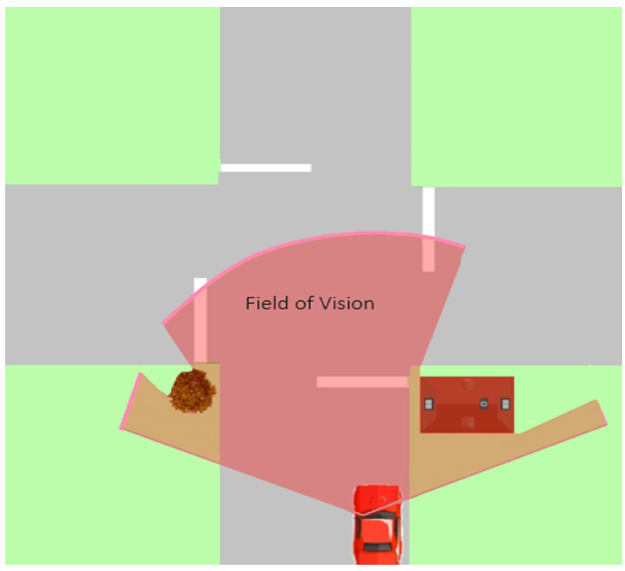
The Federal Highway Administration (FHWA) has reported that 2.4 million collisions occur at intersections every year, which accounts for about 40% of all collisions and 21.5% of traffic fatalities in the US [1]. One of the leading causes of urban intersection collisions is the failure to yield to the right of way (ROW) and restricted visibility [2]. To mitigate these visibility issues, intersection design provides provisions for minimum intersection sight distance (ISD). Sight distance is the minimum distance required by a driver to be able to effectively observe conflicting vehicles and safely complete certain maneuvers [3]. Adequate sight distance at intersections is one of the most crucial road design elements in an urban environment, which is represented by an area that needs to be clear from obstructions [4]. Figure 1 shows how road obstructions impact the driver’s visibility when a vehicle is approaching an intersection.
When a driver fails to observe a yield or stop sign at a two-way-controlled sign intersection or observe oncoming traffic from the major road due to visibility issues from the intersection, it may increase their collision risk. Sight distance is an element associated with visibility and central to the inherent safety of intersections. The ISD is specified in the road design guidelines, based on conservative values of speed, deceleration rate, perception–reaction time (PRT), and gap time acceptance. Although such distances are sufficient to ensure that drivers have a clear vision of conflicting vehicles, such minimum distances cannot always be achieved in densely built-up urban areas, and, consequently, safety problems arise at intersections. In other words, maintaining a large area clear from vegetation, buildings, or any road feature is challenging in the urban environment. Furthermore, road conditions may change during an intersection’s life cycle due to maintenance work or the installation of utilities, significantly restricting the sight distance available at the intersection.
A sight distance assessment must be conducted to assess if the sight distance at an intersection meets current guidelines, and the sight triangle is clear from obstructions in the urban environment. However, it may be ineffective to use conventional field-assessment techniques because they tend to be time-consuming, require extensive fieldwork and resources, and are of varying accuracy. More so, it may not be possible to observe all objects impacting a driver’s visibility when using different transportation modes where the driver’s height differs.
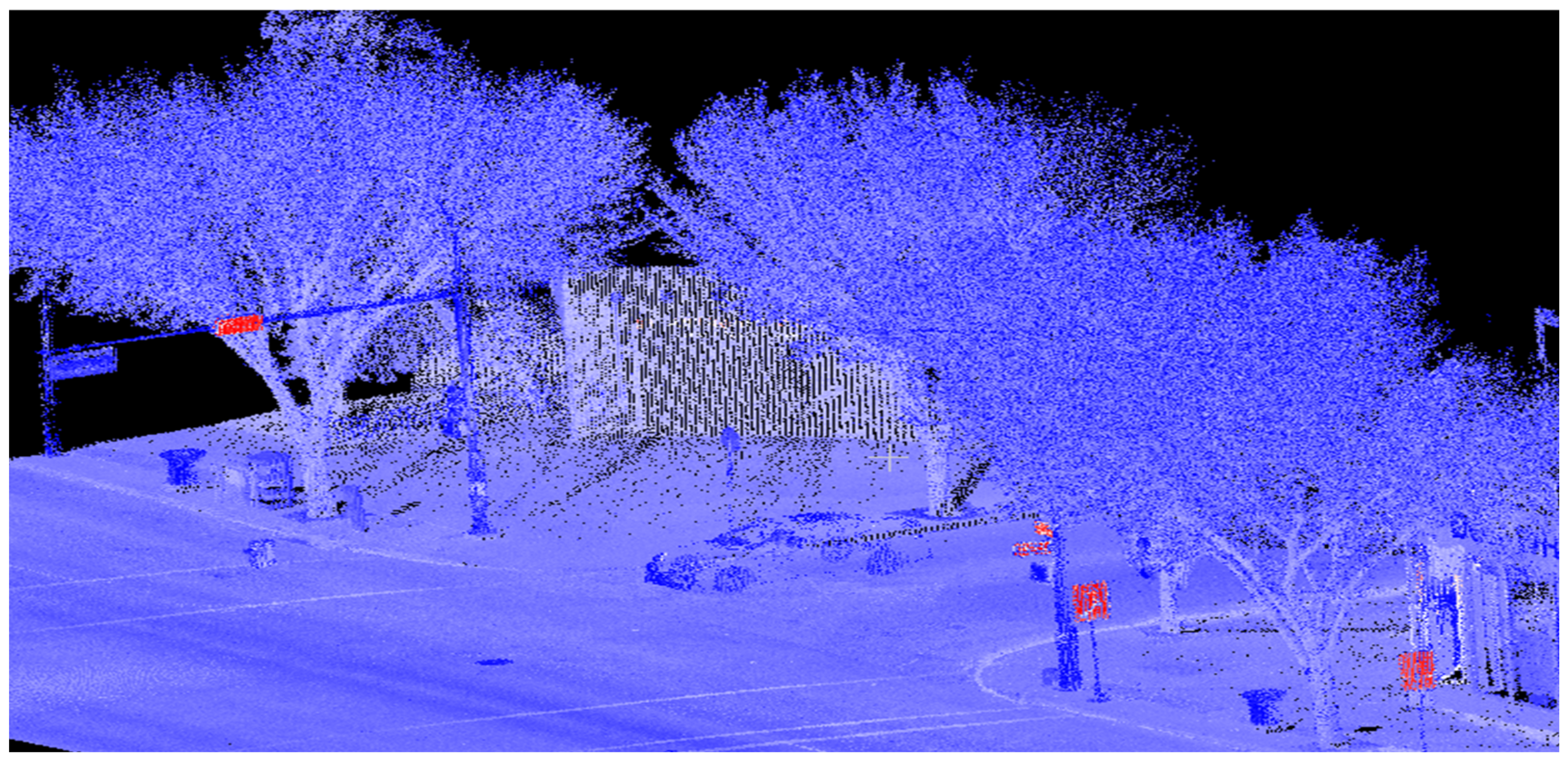
Many researchers have focused their attention on assessing road design elements using geospatial data to overcome the errors resulting from field procedures. Previous work has shown that design, terrain information [5,6], and the Digital Terrain Model (DTM) [7,8] do not accurately represent obstructions and overhanging objects that physically impact the driver’s vision by limiting the ASD. A few studies utilized Digital Surface Models (DSMs) and extracting obstacles using Geographic Information System (GIS) tools. While showing promising results, these studies involved significant manual work, site visits, and considerable time to process data due to software limitations. Moreover, detecting road obstacles through site visits is generally not an efficient way to address such issues because this is a tedious process requiring resources mobilization, obtaining a permit from authorities, providing work zone layouts, and traffic control strategies. In addition, the time and labor-intensive manual process prevents a proactive network-level analysis and exposes the workforce to high safety risks. Other limitations include low accuracy, being prone to human errors, and road closures. Hence, the advantages of using LiDAR-based methods cannot be overstated because it overcomes the limitations of manual field surveying. Moreover, with LiDAR fast scanning and automated processing at a network level, analyzing big data can reveal unprecedented insights into the relationship with collisions and allows a proactive safety audit of transportation networks. In recent decades, remote sensing has been widely used in transportation applications to mitigate the limitations found in conventional techniques. LiDAR technology has attracted significant attention for its ability to produce a visibility-related analysis that can precisely represent real-world situations in the form of a point cloud. The Mobile LiDAR Scans (MLS) produces a high level of accuracy that represents all aspects of the road and surrounding environment and thus delivers a digital twin of the scanned road [9]. It has significant potential in transforming traditional processes to enable precise, automated sight-distance assessment. It captures road infrastructure, vegetation, and existing buildings with a high level of detail, as shown in Figure 2. It facilitates sight distance assessment by extracting intersection information and detecting obstacles within the driver’s field of vision without the need for field visits or any interruption to traffic operations.
This paper proposes a unique method to mitigate previous research limitations and fill the existing gap by utilizing Mobile LiDAR data. The method develops a fully automated, novel algorithm that extracts obstacles blocking the visibility to observe conflicting vehicles by simulating the driver’s visual field, represented by raycasting sightlines. Then, the blockage rate is calculated by recording the distances for each sightline traveled and comparing it with the angular volume of the sight triangle area. The outputs provide insights into visibility at the intersection that are useful in conducting detailed collision analyses and safety assessments. This information could significantly help to prioritize intersections for improvements and select cost-effective countermeasures to enhance road safety.
2. Previous Work
With the advancement in remote sensing technology, there was a growing interest in utilizing the LiDAR in transportation applications. The use of the LiDAR and, in particular, road safety was an appealing alternative for transportation researchers due to improvements in processing times and accuracy and reductions in data collection costs [7,10]. Despite the significant potential of LiDAR, only a few studies utilized this technology to extract information about the intersection obstacle and estimate the ASD.
At the early stage, researchers tended to use LiDAR data to conduct sight distance assessments on DTM or Digital Elevation Models (DEM) using GIS. Castro, et al. [8] used ArcGIS to develop a method that evaluates existing highways’ ASD. The first step of this method starts by creating a DTM raster to calculate the viewshed with observer input. The viewsheds area was represented on the raster of visible cells, which means that it is visible to the observer. These visible areas are vectorized to produce polygons and intersect with a vehicle trajectory to obtain the available sight distance and then compare it with the result value given by highway design software (Trivium). This analysis was found to be slow and labor-intensive in the large section. There were also various locations where the viewshed analysis provided longer sight distances than the design software and found that it could better detect the vertical curves obstructions.
A few years later, Castro, et al. [11] developed a model that extracts ASD by generating a DTM from aerial LiDAR data. By using ArcGIS features, the method assessed multiple target points’ visibility to estimate the ASD and later compared the outcome with the results of Castro, et al. [8] using Kolmogorov–Smirnov and Mann–Whitney–Wilcoxon tests that did not show a significant difference. However, the authors claim that the data processing time is much faster than Castro, et al. [11]. In another study using airborne LiDAR, Castro, et al. [12] studied the impact of the successive station spacing within the vehicle path on the result of the sight distance analysis and the influence of the resolution of DTM combined with several stations and spacing distances along the roadway. Khattak, et al. [7] utilized the LiDAR elevation data to extract the intersection geometry and detect potential obstructions on driver sightlines using the GIS tools such as line of sight (LOS). Gargoum, et al. [13] proposed an algorithm to assess the stopping and passing sight distance using mobile LiDAR point cloud data in two different road segments. MLS is used to generate a DSM raster to constructLOS between the observer and target points to assess the visibility by identifying the obstruction between the LOS and surface model.
Tsai, et al. [14] assessed the ASD on intersections using LiDAR data by proposing a method to detect obstructions within the LOS manually. The method used Global Positioning System (GPS) points to represent the roadway centerlines on major corridors and intersecting roads. The sight triangles’ dimensions were estimated based on the speed limit of intersection approaches and the type of traffic control. LiDAR data were used to generate DSM to carry out sight distance analysis. A market LiDAR software was utilized to obtain a raster grid, and by overlaying the triangle area enclosed onto the DSM, visible and nonvisible pixels were identified. LiDAR assessment results were compared with the conventional site survey, which detected 92% and 64% of obstruction, respectively. The results show the effectiveness of LiDAR data to identify ISD obstructions.
Jung, et al. [15] developed an algorithm to assess the ISDusing high-resolution Mobile LiDAR data. The ground points were separated and used to determine the ground level by converting the point cloud data into 2D grids to perform LOS analysis. Then, they detected the obstructions to evaluate them in 3D space and examine the distance between the grid cell representing an obstacle to the constructed LOS. The method was successful in evaluating the sight distance obstacles. The authors indicated that the method is not applicable when the ground is in rough terrain.
Ma, et al. [16] used the airborne and terrestrial LiDAR data to propose an algorithm to estimate the 3D sight distance for stopping maneuvers in a highway with complex roadside obstacles. The method combines the modified Delaunay triangulation and cylindrical perspective to generate a vehicle trajectory along the highway with 1-m average spacing discrete points to simulate the driver’s view and generate sight distance. The result showed that there was a difference in estimating the distance when only DTM was used. The authors indicated that the method might be limited when the vehicle path and project information are not available. Moreover, the processing time was not satisfactory when processing high-density MLS data.
Shalkamy, et al. [17] developed an algorithm using mobile LiDAR to assess ASD by mapping the observers and targets onto the grid of voxels. The visibility analysis is conducted by detecting the voxel that obstructs the vector links between the observer and target points. The authors stated that the results in extracting the ASD were accurate, and the sight limitations were mainly due to the vertical crest curves and pavement surface.
In a recent study, Gargoum and Karsten [18] proposed a LiDAR-based method to assess the sight distance along a highway. The method includes discretizing the point cloud into a voxel and constructs sightlines between the observer and target point to extract and categorize the obstruction and feature available within the road alignment and roadside. The method was tested in Alberta, Canada, in four road segments and successfully quantified the highway’s available sight distance. The authors stated that the method is valuable for transportation agencies to improve road safety. However, the method cannot differentiate between the horizontal and vertical alignment along the road segment. Gouda, et al. [19,20] developed simulation-based methods for assessing ASD for autonomous vehicles using ultra-dense point cloud data.
As evident from the literature review, only a limited number of studies explored the ISD and, without extensive investigation, of collision records. Moreover, the relationship between the voxel size and extraction of road features was often unaddressed and has not been explored in detail. As such, it requires more attention to find the ideal voxel size [21,22]. One main and common limitation is neglecting the available cantilever (i.e., overhanging) objects when analyzing the data by creating DEMs, resulting in false detections and consequently biasing the visibility assessments [8,11]. This paper proposes a robust approach to querying obstructions to drivers’ field of vision at intersections. Under passenger vehicles and truck driving scenarios, the method is applied to several intersections with different control types and speed limits. The relationship between ISD and collisions is finally investigated, and a sensitivity analysis was performed to investigate the impact of voxel size on ISD. The proposed method and results provide further insights into the relationship between intersection design and road safety.
3. Visibility-Based Assessment
The method proposed in this paper is divided into two main parts. The first part, the visibility assessment, proposes a method that can be used to effectively assess, in 3D, the intersection sight distance and visibility of an urban two-way stop or yield controlled intersection. The LiDAR-based models provide high-quality information about the surrounding environment to represent the real-world situation to account for overhanging objects. This is implemented by developing a novel algorithm that facilitates fully automated extraction of the objects in the sight triangle area. This is performed by simulating the driver’s field of vision (FOV) and analyzing the driver’s sightlines in an urban intersection using high-resolution MLS to estimate the blockage rate at the intersection. This part includes a sensitivity analysis that explores the impact of voxel size on the visibility assessment that was unaddressed in literature. The second part investigates how the information obtained can be used to evaluate intersection safety. For this, ten years of historical collision records were analyzed to evaluate intersection safety by identifying hazardous intersections and study their relationship with blockage percentage.
3.1. LiDAR Data
The MLS data were collected in Edmonton, Alberta, with 54 surveys equivalent to 154 GB using a proprietary multifunction pavement surface profiling vehicle. The vehicle was equipped with RIEGL’s VUX-1HA laser scanning system with IMU (Inertial Measurement Units) and GNSS (Global Navigation Satellite System). The GNSS and IMU sensors are synchronized with the scanning system to provide accurate positional details. The system is integrated with cameras that allow the acquisition of imagery simultaneous with the captured LiDAR data in the form of panoramic images and ROW images were collected. The extraction of road features and objects in this work was developed solely using LiDAR point cloud for ISD assessment and visibility analysis. However, the video log was vital because it provides real-time supplementary information and visualization of the intersection scene (i.e., signs, posted speed, geometric characteristics, and obstacles.)
RIEGL VUX-1HA is a single scanner mobile mapping system that can perform a scanning rate of 1,000,000 measurements per second, with a scan speed of up to 250 scan lines/second, 1000 kHz effective measurement rate, and 5mm accuracy for outstanding performance in a mobile application. Several features are recorded for each point in the scan, including dense point clouds consisting of geographic, temporal, and additional attributes.
3.2. Extraction of Vehicle Trajectory
The extraction process starts by defining the trajectory points along the roadway that is parallel to the vehicle driving lane. These points are known as the position vectors, which are points used to trace the trajectory aligned with the road centerline. As shown in Figure 3, this path consists of points filtered according to the scanning angle, which has zero value, perpendicular to the scanner’s road ground, and parallel to the roadway driving axis. It is right under the scanning system on the pavement surface of the roadway toward the gravity direction. It is also known as the Nadir plane in the literature, which is opposite to the Zenith.
The algorithm allows the user to input the interval depending on the intersection location and characteristics. It is the user’s choice to select the suitable interval that represents the trajectory vector length; however, it should not be too long, in order to obtain a highly accurate result. It is worth noting that the approach where the traffic sign exists must have an active GPS time for extraction of the trajectory, which is the records the time the laser pulse was generated during the data collection and scanning process.
3.3. Voxelization of LiDAR Point Cloud
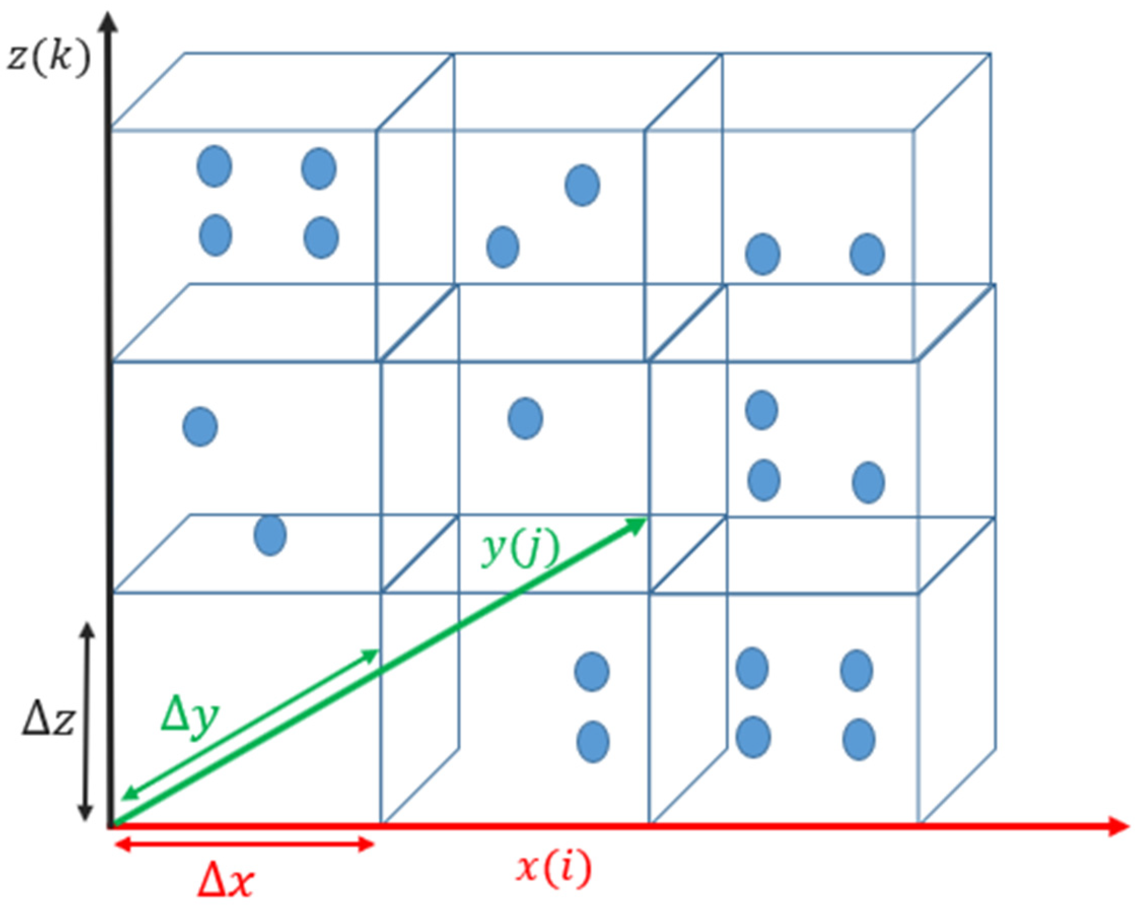
The Voxelization process was used to discretize the point cloud into a 3D grid in space to reduce the dataset volume without impacting or compromising the information [23,24,25]. This step also ensures that discretizing the LiDAR points cloud to a voxel is faster and more applicable in real-time applications that could be easily processed when comparing it to the points cloud. Dealing with large 3D data sets such as MLS requires significant processing time, and its computational cost is extremely high, which could not be practical [26]. This process also represents the LiDAR point cloud as a set of volumetric elements, which is also a known spatial grid (i.e., voxels). The voxel geometry is defined by length, width, and height. The spatial location of the voxel in the space corresponds to a 3D grid system indexed by column (i), row (j), and layer (k), as shown in Figure 4.
Each voxel in the 3D grid has a unique code known as feature ID. These voxels have their characteristics and are based on the point cloud geometrical information, as shown in Figure 5. When points correspond to the coded voxel, the value assigned to each voxel ID represents the number of point clouds falling into that voxel. Each point cloud group is assigned to pre-defined voxel IDs in space to form a high level of road feature representation.
The voxel size is vital in retaining the feature object information of the point cloud [17]. Despite that, the user can alter voxel size selection; it is recommended to choose the voxel parameters that match the scanning system characteristics and the type of application [27]. The voxel size used in this paper for the visibility assessment is 0.2 m.
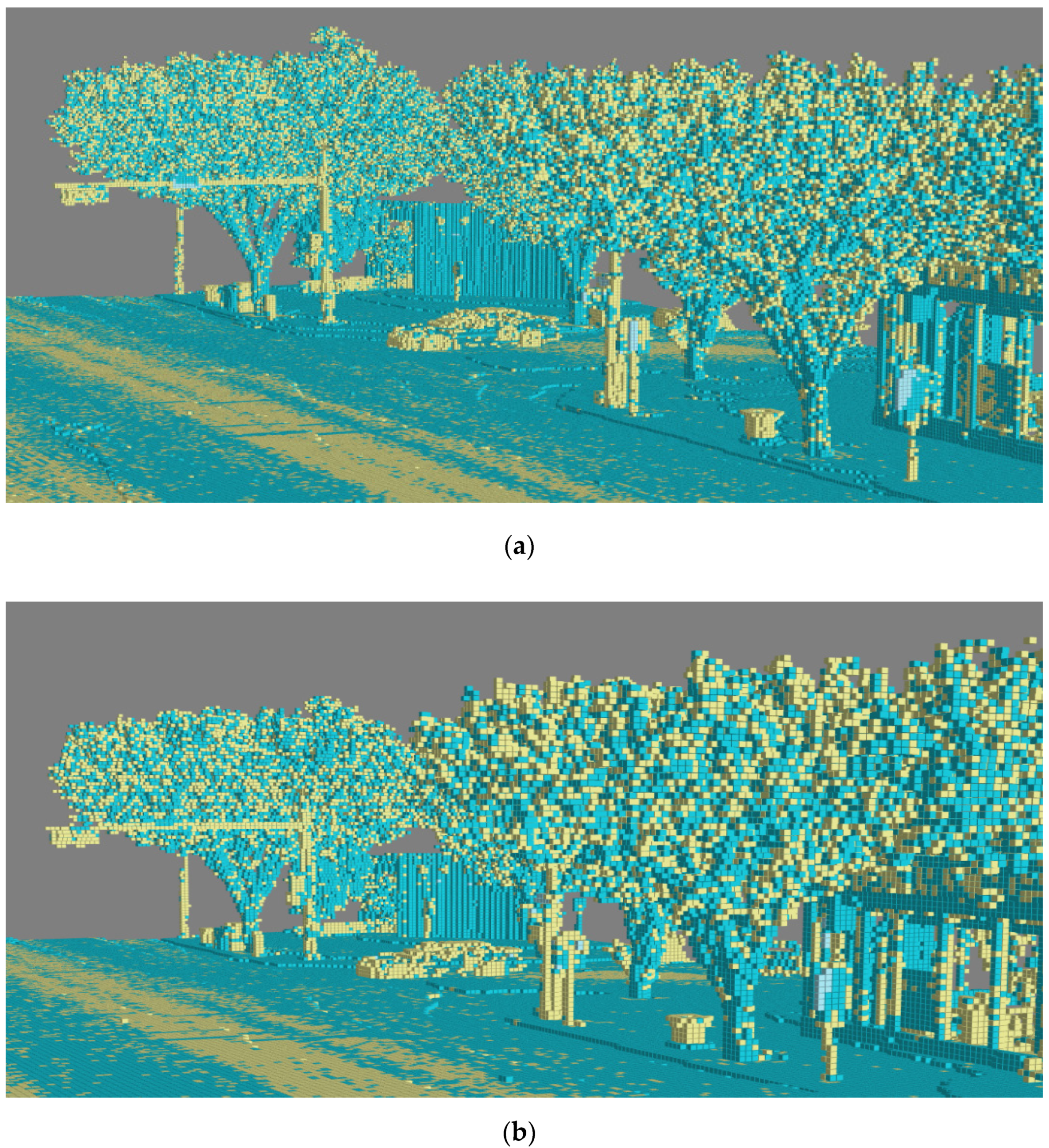
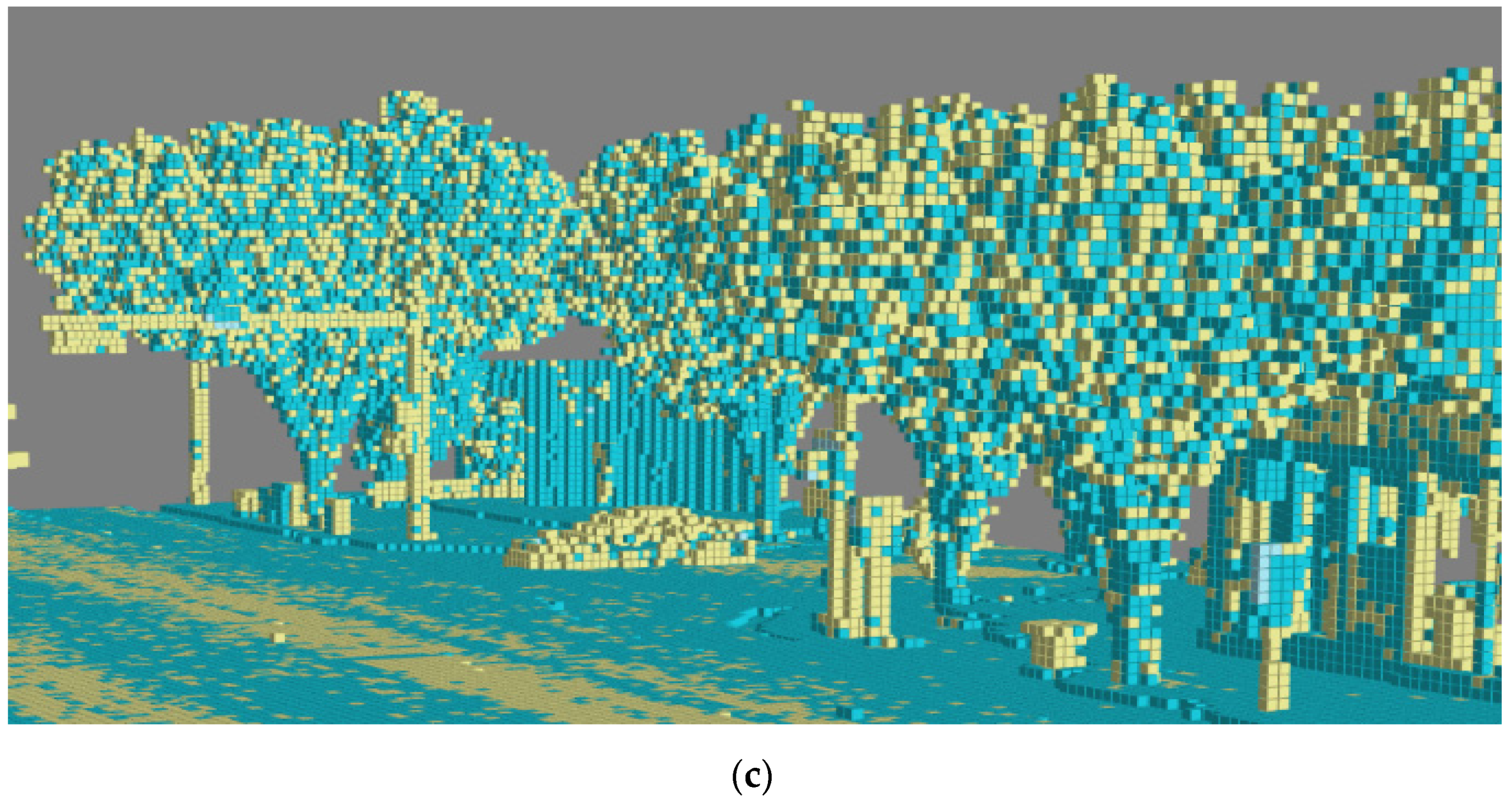
Although the variation in the voxel size is expected to influence the information extracted from the LiDAR dataset, the extent to which voxel changes could impact the extraction is questionable. Thus, the sensitivity assessment of the impact of the voxel size on the extraction quality is essential for developing an algorithm to extract information from LiDAR. In order to capture the impacts of a voxel in estimating the available sight distance, different voxel sizes were tested (0.1 m, 0.15 m, and 0.2 m), as shown in Figure 6a–c that show an intersection point cloud after voxelization with different voxel sizes.
3.4. Visual Field Assessment and Visibility Analysis
The horizontal and vertical angle parameters with their corresponding resolutions are vital in simulating the driver’s peripheral view to exploring the obstacles within the sight triangle. In this paper, the horizontal and vertical angles are considered to be 180° and 10°, respectively. A viewing angle field of vision of 140° is the minimum visual field requirement for a driver’s license in most states in the US for a person with two functioning eyes [28].
To ensure that the observer height reflects the driver’s eye level in the real-life situation and accounts for the road pavement’s rigorous surfaces, the tool uses a target offset parameter that reflects the appropriate elevation in the z-axis of the visibility analysis. To illustrate, let O be the observer point, which simulates the driver’s location. The P and Q are the following observers, each a certain level from the ground depending on the road surface but with a constant height of 1.08 m as defined in AASHTO for passenger vehicles. In the visibility analysis, the trajectory vector representing elevation is the average of the two trajectory vectors OP and PQ, which is QO.
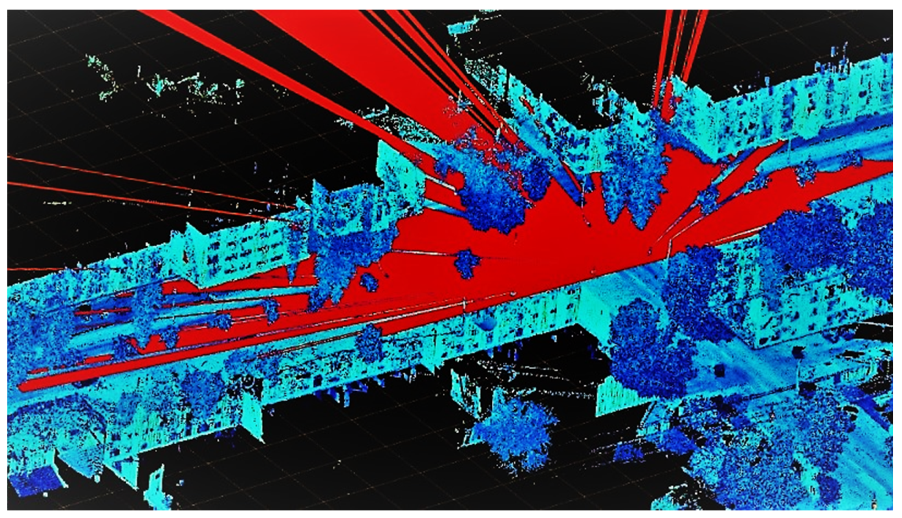
Because the MLS has a high point cloud density, the sightlines will always detect objects in the space that represent an obstruction. An effective method of extracting such objects blocking the driver’s visual field is to explore the occupied and non-occupied voxels. Any occupied voxels indicate an obstruction. The next step involves generating a visual field by sampling the line of sight used to detect objects in space from the observer points at a constant resolution angle (interval), as shown in Figure 7. The visual field is spanned by different vertical and horizontal angle pairs defined by the user. Bresenham’s algorithm is used to identify occupied voxels. The algorithm is used to compute the coordinates between the observer point and points in space representing the voxel’s edge. In other words, the straight line formulated connects the defined observer and target points. These points were selected to approximate a straight line between two points closely. Thus, when the sight line intersects with an occupied voxel at any given intersection, the voxel is queried as an obstruction.
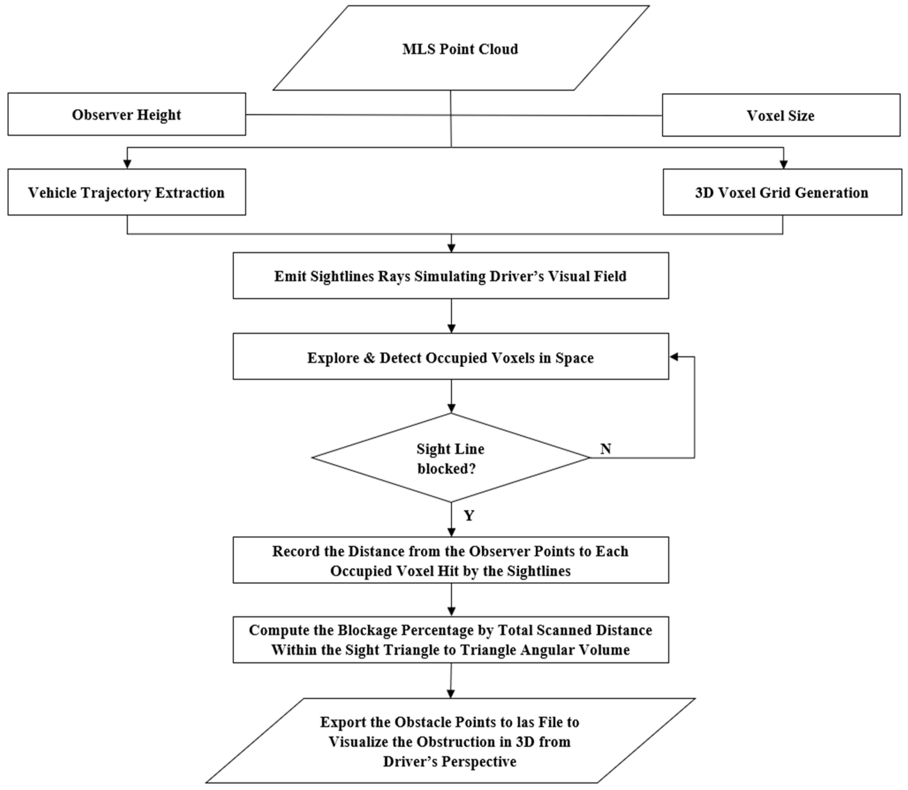
The blockage percentage is estimated by comparing the total offset distance within the sight triangle to the angular triangle area. The method also converts all points representing obstructions to a LAS file to enable the obstacle to be viewed from the driver’s perspective. The visibility assessment methodology process described above is illustrated in the flowchart shown in Figure 8.
The data was collected using RIEGL’s VUX-1HA laser scanning system, with a high density of point clouds representing the real-world environment with 5 mm accuracy. The algorithm generates the distance between the defined observer point and target point in the visibility analysis. To validate the algorithm output, distances were manually measured between these points using CloudCompare (a point cloud visualization tool) and compared to one that resulted from the algorithm. This validation technique allowed us to make sure that the algorithm computes the blockage rate with a high level of accuracy as the results were almost identical.
4. Safety-Based Assessment
4.1. Background
Research on road safety has shown how the design parameters could significantly impact collision occurrence. The sight distance design element, which is the focus of this paper, is likely to exhibit a quantitative effect on road safety. The discrepancy of previous studies on safety analysis in connection with the sight distance design element needs to be addressed [29,30,31,32,33,34,35,36]. Ten years of historical collision records were acquired from the City of Edmonton (CoE), covering the period from 2009 to 2019. Collisions occurring at intersections were analyzed to investigate the relationship with ISD.
4.2. Beta-Binomial (BB) Collision Regression Model
In this paper, the BB model is used to examine the relationship between the visibility assessment outcome and the occurrence of specific types of collisions. The Beta-Binomial is a discrete probability distribution. Vehicle entering intersections either collide or does not collide. When the collision probability is unknown, the process is known as the Bernoulli trials. The summation of these trials is represented by the binomial distribution [37]. The BB model accounts for collision data with small sample size and a low sample mean due to the large instability.
The BB model overcomes the overdispersion in data, producing a model with extra variability. The extra variability is due to the probability of Beta distribution independent event, p, that is believed to be capable of modeling a wider range of collision data [37]. Equation (1) demonstrate the extra variability of BB distribution [37]
where is the mean value of .
Following the binomial distribution, the probability of collision occurrence is as follows [38]:
where ni is defined as the total collision number at location i during a specific time; xi is the collision number of a specific collision pattern under investigation at location i from the ni collisions; i is the ratio of specific collision pattern xi to ni as a random variable; is the mean value for ; f (p) is the prior distribution with function p in the reference group.
The Beta distribution is assumed to be the prior distribution for p among the desired reference group [39]. The conventional form of the prior distribution to use in conjunction with binomial distribution in Equation (2) for observations of Beta distribution is as follows:
where α and β are prior distribution constant parameters. is the value of the Beta function at α and β given by
The mean and variance are estimated according to the characteristic of Beta distribution:
where the parameters α and β of the Beta priors distribution must be a positive value [40].
Previous research proposed a wide array of models to link collision data to several independent variables representing road features and characteristics. The most significant model to investigate specific collision patterns, which can identify the locations with an over-representation of a particular collision pattern, is the BB model. Equation (2) shows the basic structure of the BB. Following the previous derivation, the BB function can also be written by the log-likelihood as a function of . The can be linked with variable X that represent the road attributes and characteristics via the logit link [37]:
where Y = XB is the simplest safety performance function with coefficient B [37]. The maximum likelihood estimation (MLE) is used to estimate coefficient B by applying it across the BB distribution log-likelihood function. In this paper, the SAS software program was used to obtain the MLE of the function. The eventual model must be tested to ensure that the coefficients of each variable are statistically significant, and the model is a good fit for the data.
5. Results and Discussions
The visibility analysis at intersections was conducted considering different traffic control signs and transportation modes. The results show the simulated driver’s field of vision for pre-defined observer point locations, and present 2D visibility maps, and show the angle of vision where obstructions cause driver visibility problems. The 3D visualization of the driver’s visual field provides a clear image to facilitate an understanding of the obstacles to the driver’s vision and the quantification of these object positions. In addition, the results compare visibility for different transportation modes by studying the outcome and rate of blockage for a passenger vehicle and a heavy truck, each with a different observer height. Moreover, the relationship between the proportion of collisions with visibility issues and the blockage percentage is studied using Beta-Binomial (BB) collision modeling.
5.1. Visibility Assessment for Un-Signalized Intersection Using a Passenger Vehicle
When approaching an intersection controlled by a yield sign, the driver requires a certain distance to observe a potential conflicting vehicle and to slow or stop before entering the intersection, and this distance forms a large area that needs to be clear from obstruction. The AASHTO defines the area as an intersection sight triangle. This study assumed that a driver approaches the intersection to complete a left turn maneuver without stopping and needs to assess both left and right sight triangles. Therefore, the driver’s decision point begins at 25 m from the center of the lane of the vehicle approaching from the left, and this is the location when the driver starts to brake. For instance, intersection 85 Ave 100 St is two-way in both minor and major roads—with one lane in each direction—the short leg distance of the sight triangle is 28.5 m for the vehicle approaching from the right. Because the intersection is in a playground zone, the speed for both major and minor roads is 30 km/h. The ISD in the major road is determined as follows, shown in Table 1.
Using the ISD equation, the long leg of the sight triangle for both directions is 67 m considering the posted speed is 30 km/h using the time gap as defined in the AASHTO. The driver’s eye location is considered at the decision point to simulate the driver’s 3D visual field with a 1.08 m observer height. The blockage percentage is calculated based on the intersection scene by exploring the obstruction within the sight triangle from the driver’s perspective. The method also generates a visual field map of the intersection in 3D and xy-planes, showing where the sightlines intersect with obstacles.
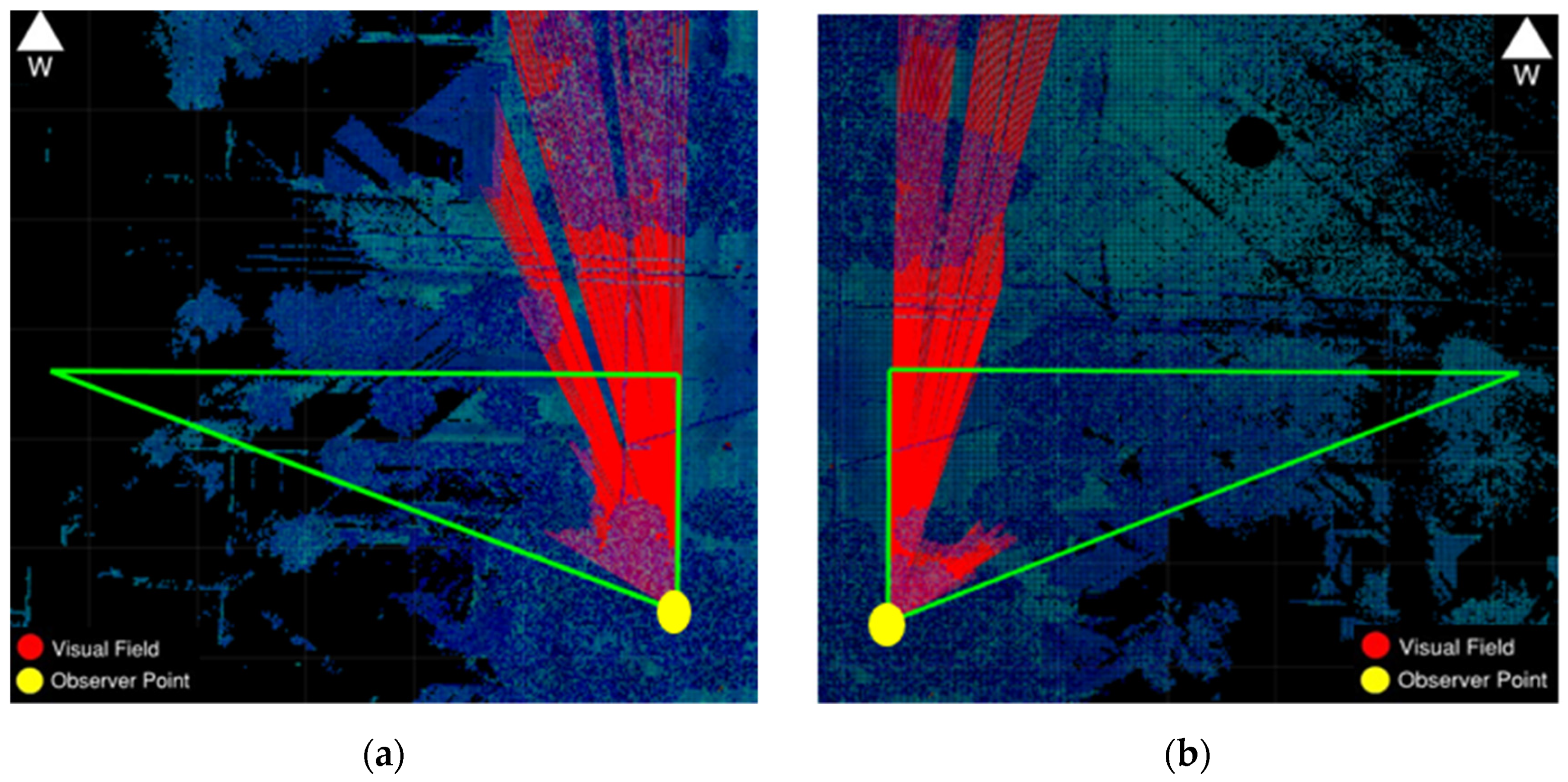
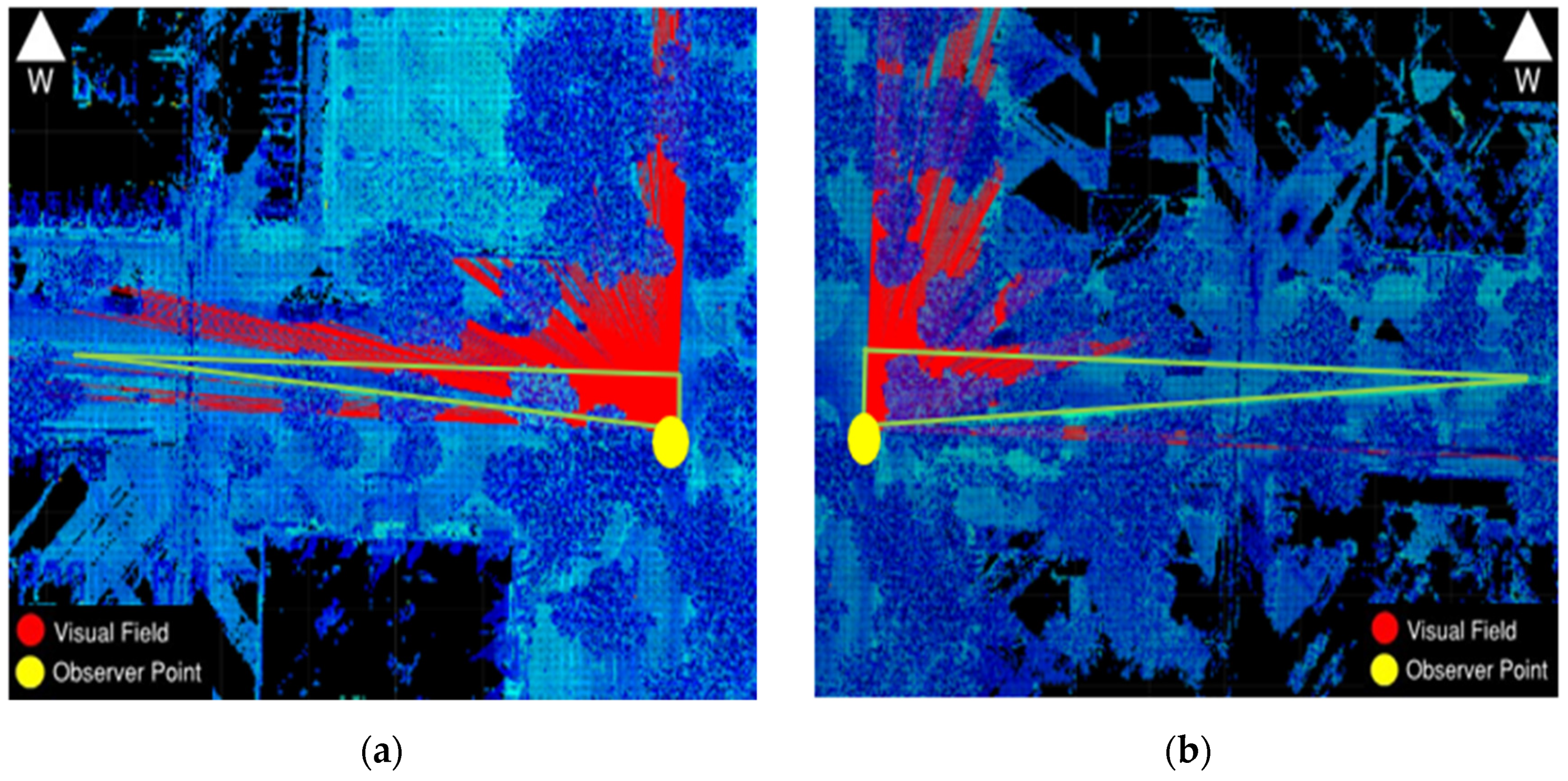
Figure 9 shows a 2D visibility map for intersection 85 Ave 100 St, and the result shows that the blockage for the left and right sight triangle is 63% and 71%, respectively. The sight triangle in green represents the area that should be clear from road obstacles and visible to the driver. The visual field is shown in red as a set of ray-cast sightlines that travel a distance defined by the user unless they intersect with an obstacle. These figures demonstrate the impact of objects such as buildings, roadside features, or bushes at an urban intersection on the driver’s ability to observe conflicting vehicles, significantly contributing to road collisions. Figure 10 shows the obstacles in red.
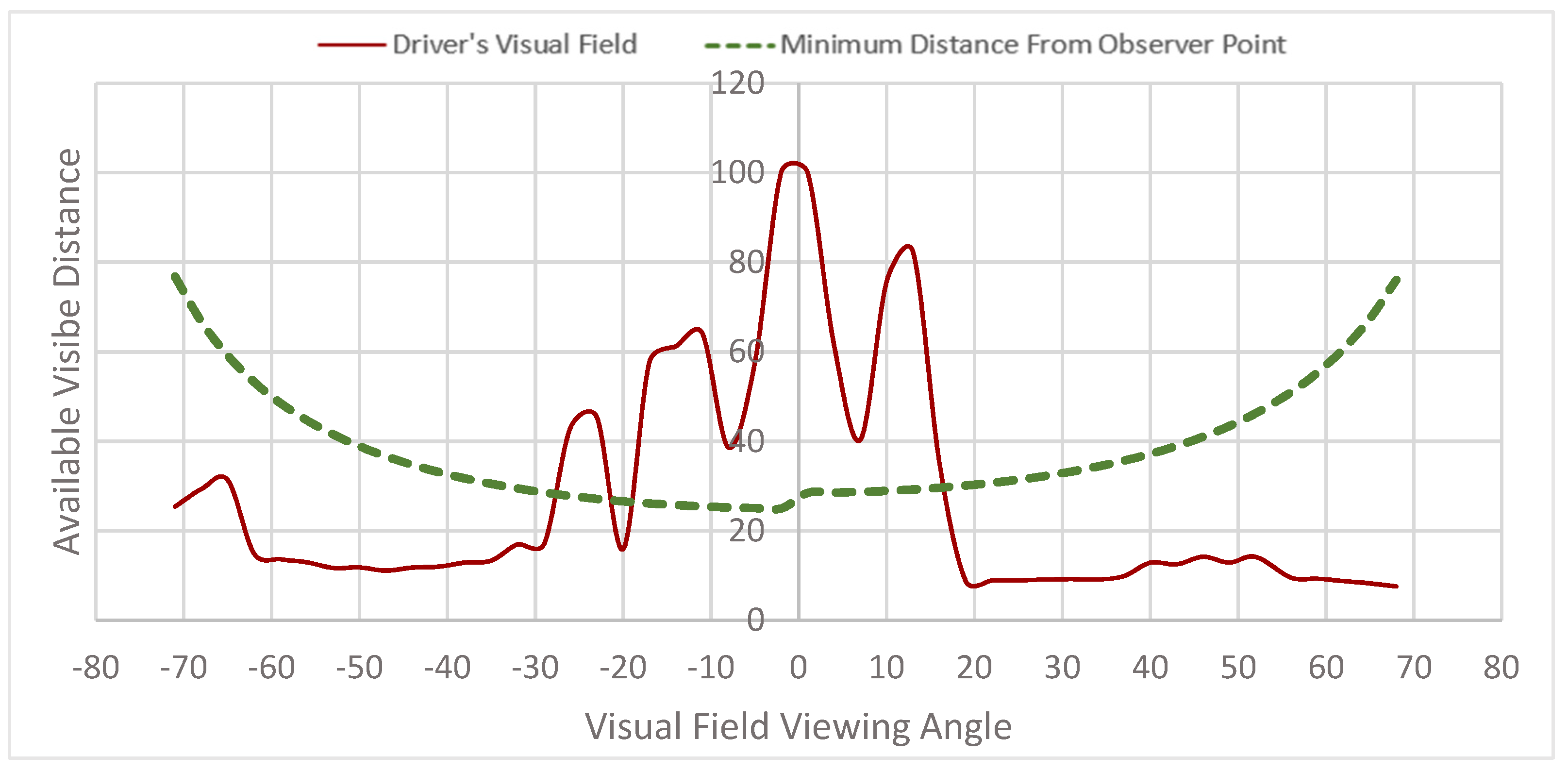
Figure 11 shows the available visible distance plots for the intersection of 85 Ave and 100 St. The dashed line drawn across the plot represents the visible distance at each viewing angle required by the AASHTO guidelines. When comparing the visual field distance and the minimum sight distance, it can be seen that the minimum distance required is met between viewing angles of −22° to −28°, and −18° to 17°; otherwise, the available sight distance is limited. The ASD decreases significantly as the viewing angle increases and does not meet the minimum required sight distance, demonstrating the high blockage percentage in a yield-controlled intersection.
For a stop-controlled intersection, the driver needs sufficient distance to stop, and observe a potential conflicting vehicle and then depart once any such vehicles are cleared. The main difference to the yield sign is that the driver must stop. The driver’s eye location is relatively close to the intersection and requires a smaller sight triangle clear from obstruction.
The driver’s decision point begins at some point between 4.4 m and 5.4 m from the major road’s intersection edge, given the vehicle stop location behind the stop line and the distance of the driver’s eye from the front of the vehicle. The gap time acceptance is 0.5 s less than for yield-controlled intersections, resulting in a shorter leg distance of the sight triangle along the major road.
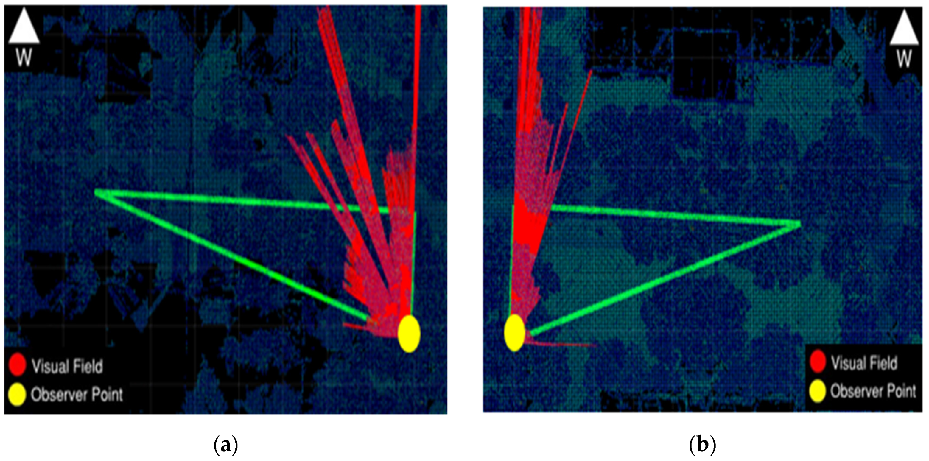
For intersection 84 Ave and 105 St, the long leg found is 105 m, given that the major and minor speeds are 50 km/h. Figure 12 shows the visibility map; the blockage percentage found in the left and right sight triangles is 27% and 40%, respectively. Generally, the results show that the blockage percentage for stop-controlled intersections is lower than for yield-controlled intersections. The reason is that the observer point is very close to the intersection, resulting in fewer obstacles.
Figure 13 shows that drivers’ ability to view oncoming vehicles on a major road to carry out certain maneuvers is undoubtedly wider in stop-controlled intersections. The plot shows that a large proportion of viewing angles met the minimum intersection sight-distance requirements. The required ISD was satisfied at viewing angles from −81° to 73° when comparing the driver’s visual field offset distance to the minimum sight distance required. The results demonstrate high levels of visibility at stop-controlled intersections, which explains the lower blockage percentage.
5.2. Visibility Assessment for Un-Signalized Intersection Using a Heavy Truck
In Section 5.1, the visibility analysis estimated the blockage percentage and visible distance across various viewing angles were based on a passenger vehicle with a lower observer height than a heavy truck. In order to assess the impact of intersection visibility on heavy truck drivers and determine the blockage percentage, visibility analyses were conducted using the same observer point locations. The principal differences compared to a passenger vehicle are the height of the observer and the time gap acceptance, which is two seconds longer for a truck. When moving onto a roadway, a truck always has a lower speed than a passenger vehicle and needs more time to enter the major road and carry out certain maneuvers. Because the long leg distance of the sight distance triangle is determined by the speed posted on the major roadway and the time gap acceptance, the sight triangle clear from obstruction required by a truck is larger than that required by a passenger vehicle.
Table 2 shows the intersection sight triangle for both yields- and stop-controlled intersections from the observer height of a heavy truck. When comparing the area of the sight triangles and the ISD, it can be noticed that for passenger vehicles, when the intersection is yield-controlled, the long leg of the sight triangle is 67 m; however, it is 84 m for trucks. The same applies to the stop-controlled sign intersection which the distance for passenger vehicle and truck is 105 m and 139 m, respectively. This demonstrates the change in the sight triangle area using a different mode of transportation.
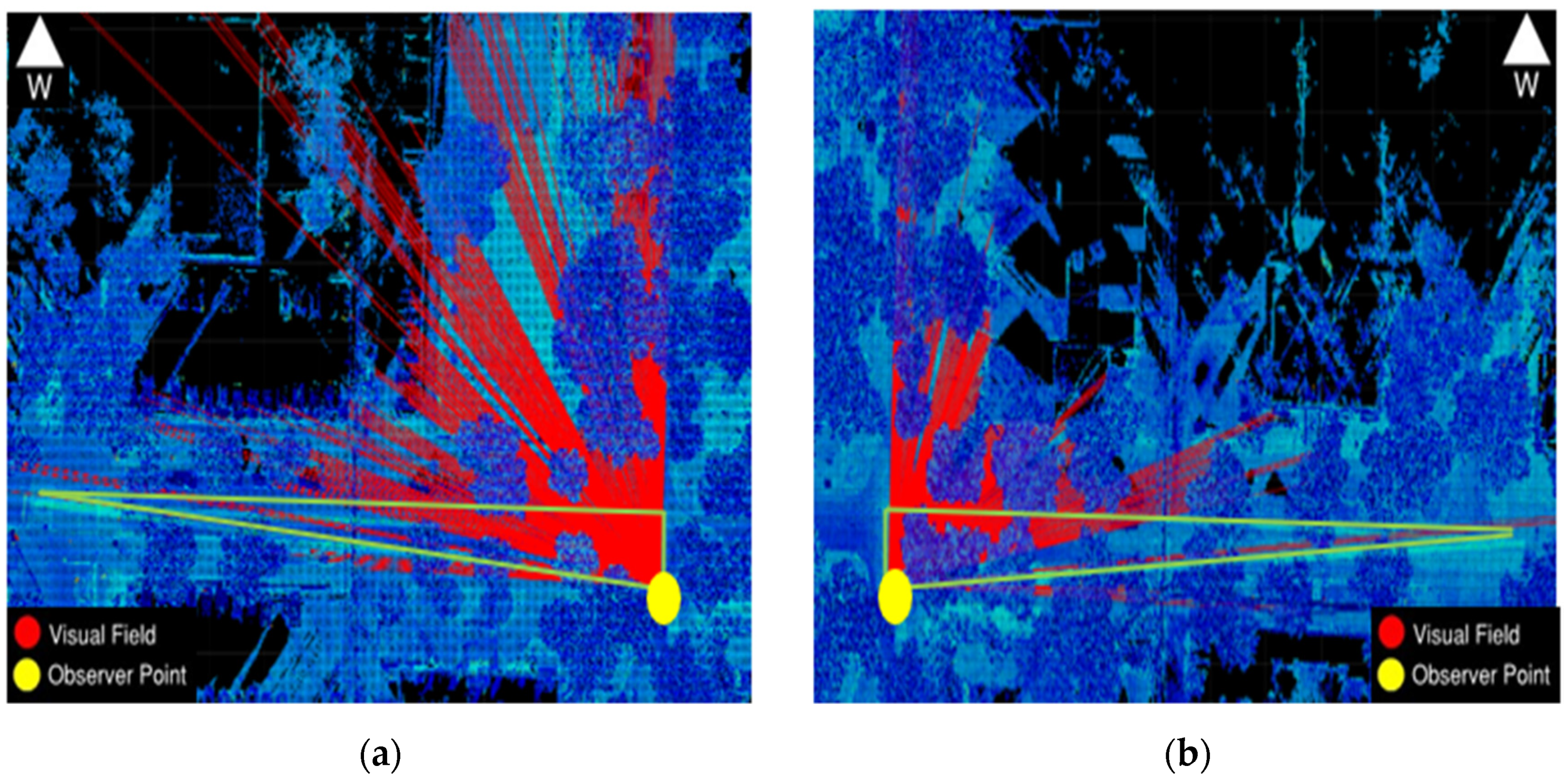
When a heavy truck approaches a yield-controlled intersection, the visibility map in Figure 14 shows that the blockage percentages for the left and right sight triangles are 70% and 77%, respectively. However, for a passenger vehicle, the equivalent figures were found to be 67% and 65%, respectively. Thus, drivers of heavy trucks approaching yield-controlled intersections in an urban environment experience slightly more blockage than passenger vehicles.
In contrast, at stop-controlled intersections, where heavy trucks are required to stop before departing, Figure 15 shows that the sightlines cover a large proportion of the sight triangle, with blockage percentages for the left and right sight triangles of only 20% and 26%, respectively. In this case, the heavy truck has a more available visible distance than the passenger car because the truck driver at the intersection has higher sightlines, allowing them a clearer view of the scene and enabling them to see oncoming vehicles on the major road.
The passenger car and heavy truck were considered in the ISD assessments to analyze the impact of observer height on visibility. The findings show that this factor contributes to variation in the blockage percentage. When the intersection is yield-controlled, more attention should be given to heavy trucks; however, the focus should be on passenger vehicles at stop-controlled intersections when assessing potential improvements to address visibility problems in an intersection’s safety performance
5.3. Impacts of Voxel Size on the Extraction Results
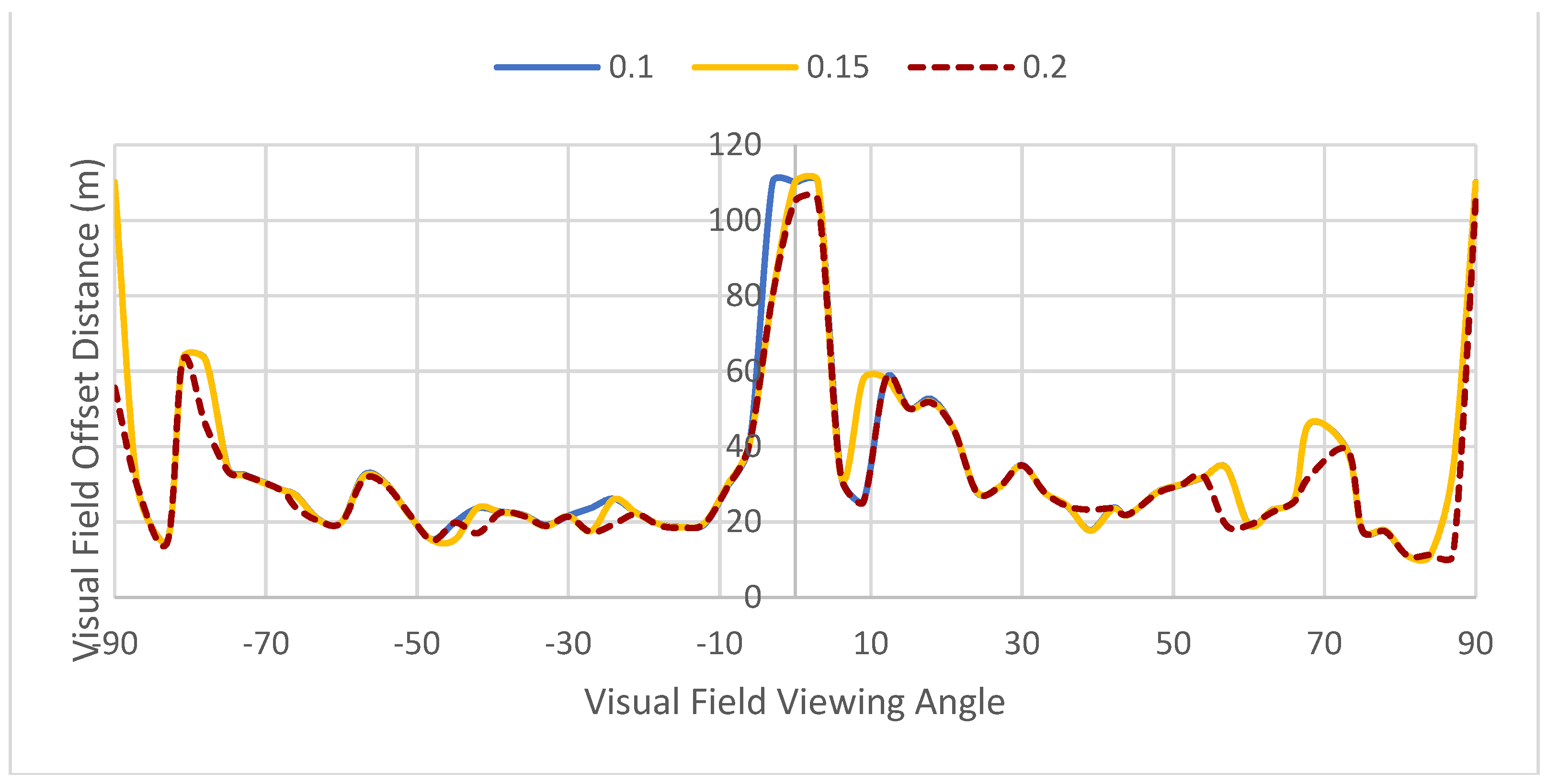
The algorithm was used to determine the offset distance in the simulated driver’s visual field at different voxel sizes. Voxel size is a sensitive parameter and an essential step of the algorithm that may influence the calculation of blockage percentages because different voxel sizes result in different visual field distances and therefore impact the quality of the information derived from the visibility assessment. As an illustration, 84 Ave 105 St intersection was analyzed at different voxel sizes to demonstrate the impact of voxel size on the assessment. The plots in Figure 16 and Figure 17 show the distance that the driver can see at various viewing angles and considering different voxel sizes. The plots show that each intersection, irrespective of voxel size, shows similar trends and exhibits only a slight variation in offset distance.
Although the plots show the estimated sightline distances at different voxel sizes to be very similar, this variation in distance needs to be quantified. To understand the impact of voxel size and address these variations in the visibility assessment, the difference in each sightline of the visual field at a defined observer point with a different viewing angle was compared to the estimated sightlines at a voxel size of 0.2 m. The plot in Figure 18 for intersection 84 Ave 105 St is the average difference in sightline distance measured in meters at different voxel sizes.
The variation in the estimated distances demonstrates that reducing the voxel size results in an increase in visual field offset distance and provides a greater field of view. The increase varies depending on the voxel size used in the analysis; however, the estimated average increase ranges from 3.3 m to 4 m. Moreover, the plots show a boost when voxel size decreases. Reducing the voxel size from 0.2 m to 0.1 m results in eight times as many voxels. Thus, when the size of the voxel is 0.2 m and contains one point, this voxel is occupied and represents a road obstacle, and when the sightline hits this voxel, it stops traveling to explore other voxels. A reduced voxel size of 0.1 m results in eight voxels of 0.1 m, equivalent to one voxel of 0.2 m in size. In the same situation, one voxel out of eight will be occupied, while the others will be visible.
In fact, the impact of the change of voxel size on the performance of the intersection assessment tool was minimal. However, other transportation applications may be highly sensitive to voxel size, which may impact the accuracy of the information extracted. The outcome of this sensitivity analysis demonstrates that the use of a finer voxel size is not always necessary. In other words, the research shows that the algorithm for the extraction of obstacles within intersection sight distance remains effective when using slightly larger voxels with no significant effect on the quality of the information obtained.
The use of a smaller voxel size would significantly increase the processing time for extraction, especially when working with the high point density of MLS, which may be costly. In this study, the density of the point cloud ranges from 43.6 million to 76.4 million.
5.4. Beta-Binomial (BB) Regression Model
This method examines the relationship between collision history and visibility problems through regression modeling. Because this study is focused on investigating specific collision patterns, BB distribution was proposed to develop a collision model to link the collision proportion and blockage percentage.
In the first step, the collision proportion was calculated for each intersection, according to the given data, and set as a dependent variable (CP). Because the study investigates the impact of poor visibility, the blockage rate was regarded as the independent variable (B). The computational software program SAS was used to develop a collision model [41]. The BB model coefficients were computed using a finite mixture of univariate distributions in SAS: “The FMM Procedure”.
Referring to the model output as shown in Table 3 and Table 4, coefficient B was statistically significant because the Pr value is lower than the 0.05 significance level. For the goodness-of-fit model assessment, Maximum Log-Likelihood Estimation was used. Pearson’s chi-squared measure, shown in the model as the “Pearson Statistic,” must be compared with the tabulated chi-squared value. Because one coefficient is considered in the model and has 26 site observations, the degree of freedom (DF) is equal to 25. Therefore, the tabulated chi-squared distribution value is equal to 14.611, which is greater than the Pearson Statistics output of the regression model. Thus, the model regression coefficients and the goodness of fit are found to be statistically significant.
The results of the BB model indicate that the collision proportion increases as the blockage rate increases. As a result, the safety assessment finds that locations with restricted sightlines due to road obstacles at intersections were at increased risk of collisions; thus, limited available visible distance contributed to collision occurrences. Therefore, identifying a design deficiency—such as limited sight distance at an intersection—and linking it with the collision record to generate a function that explains the relationship with collision occurrence would significantly help traffic safety professionals choose cost-effective countermeasure to improve visibility such intersections.
6. Conclusions
The paper proposed an automated method to facilitate visibility assessment at urban intersections. This is performed by extracting the vehicle trajectory and simplifying the data into voxels representing the point clouds. It estimates blockage rate within the intersection sight triangle by detecting the obstacles that block the driver’s visual field. This analytical approach can assist in improving intersection visibility by enhancing drivers’ field of vision without the burden of manual techniques. Traditional processes are tedious and require a substantial on-site resource to carry out field surveying work, including equipment and tools that may affect the traffic operation and lead to unsafe situations that impact the road users and field surveyors.
The proposed work supports agencies in the transportation field in assessing available intersection sight distance and identify hazardous intersections where visibility should be improved. It also provides high-quality information about the intersection characteristics and the location of obstacles. Having such information on a large scale helps assets and maintenance management teams adopt policies and make decisions to improve road safety by improving the field of vision at urban intersections, significantly and cost-effectively decreasing the occurrence of collisions.
Selecting the ideal voxel size is critical in obtaining accurate extraction of information. To address this, a sensitivity analysis was conducted using various voxel sizes. While voxel size does not significantly impact this sight distance application, it may be very sensitive to extract different geometric road features in other transportation applications [42]. In other words, the selection of an inappropriate voxel size leads to minor inaccuracies in detecting obstacles. These findings help agencies with a limited budget work with this kind of dataset without investing in a powerful computing server.
LiDAR is commonly promoted as a feasible option when network-level infrastructure management is the target. On the other hand, if a project target studying a few intersections, LiDAR may be an expensive option. It is important to note that with advances in LiDAR technology and deployment of autonomous/connected vehicles, crowdsourcing point cloud scans will be a byproduct of autonomous vehicles, and data will be readily available for a far lower cost.
There are limitations that can be explored in future studies. For instance, all approaches of the intersections included in our study were perpendicular. Applying the analysis to skewed intersections can reveal further insights into the relationship with collisions. Future research also recommends exploring the impact of other factors (e.g., maintenance activities) if data is available [43]. The age of drivers has an influence on their visual field, and their impacts have not been considered in the study. In addition, the selection of an inappropriate voxel size could lead to minor inaccuracies in detecting obstacles. Developing new methods that can operate directly on points without transformation to volumetric representations is suggested. Voxel assessment limitations could be avoided by using a point-based isovist method. The method also can be enhanced for application in autonomous vehicle (AV) environments. One such recent application is the use of point clouds to simulate AVs’ movement in virtual reality using twin scans of the existing environment and assess readiness for the deployment of future technologies in a shared environment between active modes of transportation and automated vehicles [19,20].
Author Contributions
Conceptualization, O.K., M.G. and K.E.-B.; methodology, O.K. and M.G.; software, J.W., O.K. and M.G.; validation, O.K.; formal analysis, O.K.; investigation, O.K.; resources, K.E.-B.; data curation, O.K.; writing—original draft preparation, O.K.; writing—review and editing, O.K., M.G. and K.E.-B.; visualization, O.K. and K.E.-B.; supervision, K.E.-B.; project administration, K.E.-B.; funding acquisition, K.E.-B. All authors have read and agreed to the published version of the manuscript.
Funding
This research was funded by the Natural Sciences and Engineering Research Council of Canada (NSERC).
Institutional Review Board Statement
Not applicable.
Informed Consent Statement
Not applicable.
Data Availability Statement
The data that support the findings of this study are available from the City of Edmonton. Restrictions apply to the availability of these data, which were used under license for this study.
Acknowledgments
The contents of this paper reflect the views of the authors who are responsible for the facts and the accuracy of the data presented herein. The contents do not necessarily reflect the official views or policies of the City of Edmonton. We acknowledge the support of the Natural Sciences and Engineering Research Council of Canada (NSERC). Cette recherche a été financée par le Conseil de recherches en sciences naturelles et en génie du Canada (CRSNG).
Conflicts of Interest
The authors declare no conflict of interest.
References
- The National Intersection Safety Problem [Issue Briefs Vol. 2]. 2009. Available online: https://rosap.ntl.bts.gov/view/dot/49962 (accessed on 15 August 2021).
- NHTSA. Crash Factors in Intersection-Related Crashes: An On-Scene Perspective; NHTSA: Washington, DC, USA, 2010.
- American Association of State Highway and Transportation Officials (AASHTO). A Policy on Geometric Design of Highways and Streets, 7th ed.; AASHTO: Washington, DC, USA, 2018. [Google Scholar]
- PIARC. Road Safety Manual 2003. Available online: https://www.piarc.org/en/PIARC-knowledge-base-Roads-and-Road-Transportation/Road-Safety-Sustainability/Road-Safety/safety-manual (accessed on 15 August 2021).
- Ismail, K.; Sayed, T. New Algorithm for Calculating 3D Available Sight Distance. J. Transp. Eng. 2007, 133, 572–581. [Google Scholar] [CrossRef]
- Hassan, Y.; Easa, S.; Halim, A. Sight distance on horizontal alignments with continuous lateral obstructions. Transp. Res. Rec. J. Transp. Res. Board 1995, 1500, 31–42. [Google Scholar]
- Khattak, A.J.; Hallmark, S.; Souleyrette, R. Application of Light Detection and Ranging Technology to Highway Safety. Transp. Res. Rec. 2003, 1836, 7–15. [Google Scholar] [CrossRef]
- Castro, M.; Iglesias, L.; Sánchez, J.A.; Ambrosio, L. Sight distance analysis of highways using GIS tools. Transp. Res. Part C Emerg. Technol. 2011, 19, 997–1005. [Google Scholar] [CrossRef]
- Castro, M.; Lopez-Cuervo, S.; Paréns-González, M.; de Santos-Berbel, C. LIDAR-based roadway and roadside modelling for sight distance studies. Surv. Rev. 2016, 48, 309–315. [Google Scholar] [CrossRef]
- Gouda, M.; Mello, B.A.A.; El-Basyouny, K. Automated Safety Assessment of Roadside Clear Zones using LiDAR Data. Transp. Res. Rec. J. Transp. Res. Board Press 2021. [Google Scholar] [CrossRef]
- Castro, M.; Anta José, A.; Iglesias, L.; Sánchez José, A. GIS-Based System for Sight Distance Analysis of Highways. J. Comput. Civ. Eng. 2014, 28, 04014005. [Google Scholar] [CrossRef]
- Castro, M.; Garcia-Espona, A.; Iglesias, L. Terrain Model Resolution Effect on Sight Distance on Roads. Period. Polytech. Civ. Eng. 2015, 59, 165–172. [Google Scholar] [CrossRef] [Green Version]
- Gargoum, S.; El-Basyouny, K.; Sabbagh, J. Assessing Stopping and Passing Sight Distance on Highways Using Mobile LiDAR Data. J. Comput. Civ. Eng. 2018, 32, 04018025. [Google Scholar] [CrossRef]
- Tsai, Y.; Yang, Q.; Wu, Y. Use of Light Detection and Ranging Data to Identify and Quantify Intersection Obstruction and Its Severity. Transp. Res. Rec. 2011, 2241, 99–108. [Google Scholar] [CrossRef]
- Jung, J.; Olsen, M.J.; Hurwitz, D.S.; Kashani, A.G.; Buker, K. 3D virtual intersection sight distance analysis using lidar data. Transp. Res. Part C: Emerg. Technol. 2018, 86, 563–579. [Google Scholar] [CrossRef]
- Ma, Y.; Zheng, Y.; Cheng, J.; Easa, S. Real-Time Visualization Method for Estimating 3D Highway Sight Distance Using LiDAR Data. J. Transp. Eng. Part A: Syst. 2019, 145, 04019006. [Google Scholar] [CrossRef]
- Shalkamy, A.; El-Basyouny, K.; Xu, H.Y. Voxel-Based Methodology for Automated 3D Sight Distance Assessment on Highways using Mobile Light Detection and Ranging Data. Transp. Res. Rec. 2020, 2674, 587–599. [Google Scholar] [CrossRef]
- Gargoum, S.A.; Karsten, L. Virtual assessment of sight distance limitations using LiDAR technology: Automated obstruction detection and classification. Autom. Constr. 2021, 125, 103579. [Google Scholar] [CrossRef]
- Gouda, M.; Mirza, J.; Weiß, J.; Castro, A.R.; El-Basyouny, K. Octree-Based Point Cloud Simulation to Assess the Readiness of Highway Infrastructure for Autonomous Vehicles. Comput. Aided Civ. Infrastruct. Eng. 2021, 36, 922–940. [Google Scholar] [CrossRef]
- Gouda, M.; Chowdhury, I.; Weiß, J.; Epp, A.; El-Basyouny, K. Automated Assessment of Infrastructure Preparedness for Autonomous Vehicles. Autom. Constr. 2021, 129, 103820. [Google Scholar] [CrossRef]
- Pyysalo, U. Viewshed Analysis And Visualization of Landscape Voxel Models. Available online: https://www.semanticscholar.org/paper/VIEWSHED-ANALYSIS-AND-VISUALIZATION-OF-LANDSCAPE-Pyysalo-Pyysalo/53102488d6aec8a32c3fce64e9aad69d398b3691 (accessed on 15 August 2021).
- Hagstrom, S. Voxel-Based LIDAR Analysis and Applications. Available online: https://www.semanticscholar.org/paper/Voxel-Based-LIDAR-Analysis-and-Applications-Hagstrom/9486324dc24b81519c2c50a8a9149aa7e7a55085 (accessed on 15 August 2021).
- Cabo, C.; Ordoñez, C.; García-Cortés, S.; Martínez, J. An algorithm for automatic detection of pole-like street furniture objects from Mobile Laser Scanner point clouds. ISPRS J. Photogramm. Remote Sens. 2014, 87, 47–56. [Google Scholar] [CrossRef]
- Yang, B.; Dong, Z.; Zhao, G.; Dai, W. Hierarchical extraction of urban objects from mobile laser scanning data. ISPRS J. Photogramm. Remote Sens. 2015, 99, 45–57. [Google Scholar] [CrossRef]
- Yadav, M.; Lohani, B.; Singh, A.K.; Husain, A. Identification of pole-like structures from mobile lidar data of complex road environment. Int. J. Remote Sens. 2016, 37, 4748–4777. [Google Scholar] [CrossRef]
- Aijazi, A.; Checchin, P.; Trassoudaine, L. Segmentation Based Classification of 3D Urban Point Clouds: A Super-Voxel Based Approach with Evaluation. Remote Sens. 2013, 5, 1624–1650. [Google Scholar] [CrossRef] [Green Version]
- Gargoum, S.A.; Koch, J.C.; El-Basyouny, K. A Voxel-Based Method for Automated Detection and Mapping of Light Poles on Rural Highways using LiDAR Data. Transp. Res. Rec. 2018, 2672, 274–283. [Google Scholar] [CrossRef]
- Bhise, V. Ergonomics in the Automotive Design Process; CRC Press, Taylor & Francis: Boca Raton, FL, USA, 2012. [Google Scholar]
- Babkov, V. Road Conditions and Traffic Safety. Transp. Res. Board 1975. Available online: https://trid.trb.org/view/41860 (accessed on 15 August 2021).
- Deng, K.; Zhang, H.; Huang, Y. Safety Analysis on Road Sight Distance. In Proceedings of the 2008 International Conference on Intelligent Computation Technology and Automation (ICICTA), Changsha, China, 20–22 October 2008; pp. 461–465. [Google Scholar]
- Olson, P.L.; Cleveland, D.E.; Fancher, P.S.; Kostyniuk, L.P.; Schneider, L.W. Parameters Affecting Stopping Sight Distance; National Cooperative Highway Research Program Report 270; National Research Council: Washington, DC, USA, 1984. [Google Scholar]
- Sparks, W.J. The Influence of highway characteristics on accident rates. Public Work. 1968, 99, 101–103. [Google Scholar]
- Fambro, D.; Urbanik, T.; Hinshaw, W.; Hanks, J.W.; Ross, M.; Tan, C.H.; Pretorius, C. Stopping Sight Distance Considerations At Crest Vertical Curves On Rural Two-Lane Highways In Texas; Final Report; Texas Transportation Institute, Texas A&M University System: College station, TX, USA, 1989. [Google Scholar]
- Urbanik, T., II; Hinshaw, W.; Fambro, D.B. Safety Effects of Limited Sight Distance on Crest Vertical Curves; Transportation Research Record No. 1208; Transportation Research Board: Washington, DC, USA, 1989; Available online: http://onlinepubs.trb.org/Onlinepubs/trr/1989/1208/1208-004.pdf (accessed on 15 August 2021).
- Coburn, T.M. The Relation Between Accidents and Layout on Rural Roads. In Proceedings of the 1st Australian Road Research Board (ARRB) Conference, Canberra, Australia, 1962; pp. 502–509. Available online: https://trid.trb.org/View/1209092 (accessed on 15 August 2021).
- Fitzpatrick, K.; Fambro, D.; Stoddard, A. Safety Effects of Limited Stopping Sight Distance on Crest Vertical Curves. Transp. Res. Rec. 2000, 1701, 17–24. [Google Scholar] [CrossRef]
- Tong, J.; Lord, D. Investigating the Application of Beta-Binomial Models in Highway Safety. Available online: https://www.semanticscholar.org/paper/Investigating-the-application-of-beta-binomial-in-Tong-Lord/31bacbd2e3a97b5462f91b22bdf9d7b40432e195 (accessed on 15 August 2021).
- Garren, S.; Smith, R.; Piegorsch, W. Bootstrap Goodness-of-Fit Test for the Beta-Binomial Model. J. Appl. Stat. 2000, 28. [Google Scholar] [CrossRef]
- Maritz, J.S.; Lwin, T. Empirical Bayes Methods, 2nd ed.; Chapman and Hall: London, UK, 1989; pp. 88–102. [Google Scholar]
- Sayed, T.; Navin, F.; Abdelwahab, W. A countermeasure-based approach for identifying and treating accident prone locations. Can. J. Civ. Eng. 2011, 24, 683–691. [Google Scholar] [CrossRef]
- SAS Institute Inc. SAS OnDemand for Academics. Available online: https://www.sas.com/en_ca/software/on-demand-for-academics.html#windows (accessed on 15 August 2021).
- Agina, S.; Shalkamy, A.; Gouda, M.; El-Basyouny, K. Automated Assessment of Passing Sight Distance on Rural Highways using Mobile LiDAR Data. Transp. Res. Rec. 2021, 03611981211031235. [Google Scholar] [CrossRef]
- Gouda, M.; El-Basyouny, K. Before-and-After Empirical Bayes Evaluation of Achieving Bare Pavement using Anti-Icing on Urban Roads. Transp. Res. Rec. 2020, 2674, 92–101. [Google Scholar] [CrossRef]
Figure 1.
Driver’s Field of Vision.

Figure 2.
LiDAR Point Cloud in Edmonton, Alberta.

Figure 3.
Vehicle Trajectory.

Figure 4.
Voxels for point cloud in space.

Figure 5.
LiDAR Point Cloud.

Figure 6.
Different Voxel Sizes in Space (a) voxel size 0.1 m; (b) Voxel Size 0.15 m; (c) Voxel Size 0.2 m.
Figure 6.
Different Voxel Sizes in Space (a) voxel size 0.1 m; (b) Voxel Size 0.15 m; (c) Voxel Size 0.2 m.


Figure 7.
The simulated field at an urban intersection.

Figure 8.
Proposed method flow chart.

Figure 9.
Visibility Map (Intersection 85 Ave and 100 St) (a) left sight triangle blockage percentage 63%; (b) right sight triangle blockage percentage 71%.
Figure 9.
Visibility Map (Intersection 85 Ave and 100 St) (a) left sight triangle blockage percentage 63%; (b) right sight triangle blockage percentage 71%.

Figure 10.
Obstructions in a 3D Scene (Intersection 85 Ave and 100 St).

Figure 11.
Available Visible Distance (Intersection 85 Ave and 100 St).

Figure 12.
Visibility Map (Intersection 84 Ave and 105 St) (a) left sight triangle blockage percentage 27%; (b) right sight triangle blockage percentage 40%.
Figure 12.
Visibility Map (Intersection 84 Ave and 105 St) (a) left sight triangle blockage percentage 27%; (b) right sight triangle blockage percentage 40%.

Figure 13.
Available Visible Distance (Intersection 84 Ave & 105 St).

Figure 14.
Visibility Map (Intersection 85 Ave and 101 St) (a) left sight triangle blockage percentage 70%; (b) right sight triangle blockage percentage 77%.
Figure 14.
Visibility Map (Intersection 85 Ave and 101 St) (a) left sight triangle blockage percentage 70%; (b) right sight triangle blockage percentage 77%.

Figure 15.
Visibility Map (Intersection 84 Ave and 105 St) (a) left sight triangle blockage percentage 20%; (b) right sight triangle blockage percentage 26%.
Figure 15.
Visibility Map (Intersection 84 Ave and 105 St) (a) left sight triangle blockage percentage 20%; (b) right sight triangle blockage percentage 26%.

Figure 16.
Available Visible Distance Estimated at Different Voxel Size (Intersection 84 Ave and 105 St) (a) 0.1 m voxel size; (b) 0.15 m voxel size; (c) 0.2 m voxel size.
Figure 16.
Available Visible Distance Estimated at Different Voxel Size (Intersection 84 Ave and 105 St) (a) 0.1 m voxel size; (b) 0.15 m voxel size; (c) 0.2 m voxel size.

Figure 17.
Available Visible Distance Multi-voxel size (Intersection 84 Ave and 105 St).

Figure 18.
Average Difference in Estimated Visual Field Distance Compared to 0.2 m voxel size.


Table 1.
Intersection Sight Distance (ISD) [3].
Table 1.
Intersection Sight Distance (ISD) [3].
| US Customary | Metric |
|---|---|
| ISD = intersection sight distance (length of the leg of sight triangle along the major road) (ft) | ISD = intersection sight distance (length of the leg of sight triangle along the major road) (m) |
| Vmajor = design speed of major road (mph) | Vmajor = design speed of major road (km/h) |
| tg = time gap for a minor road vehicle to enter the major road (s) | tg = time gap for a minor road vehicle to enter the major road (s) |
Table 2.
Intersection Sight Triangle.
| Sight Triangle | Short Leg (m) | Long Leg (m) | |||||
|---|---|---|---|---|---|---|---|
| Intersection | Major Speed | Minor Speed | Sign | Approach | Left Triangle | Right Triangle | Left & Right Triangles |
| (km/h) | (km/h) | ||||||
| 85 Ave & 101 St | 30 | 30 | Yield | East | 25 | 28.5 | 84 |
| 84 Ave & 105 St | 50 | 50 | Stop | East | 7.2 | 10.5 | 139 |
Table 3.
Parameter estimates for BB Model.
| Effect | Estimate | Standard Error | z-Value | |
|---|---|---|---|---|
| Intercept | −2.5822 | 1.2487 | −2.07 | 0.0387 |
| B | 2.398 | 1.123 | 2.14 | 0.0327 |
Table 4.
The goodness of fit estimation value.
| Fit Statistics | −2 Log-Likelihood | Pearson Statistics |
|---|---|---|
| Value | 23.5001 | 8.0387 |
Publisher’s Note: MDPI stays neutral with regard to jurisdictional claims in published maps and institutional affiliations. |
© 2021 by the authors. Licensee MDPI, Basel, Switzerland. This article is an open access article distributed under the terms and conditions of the Creative Commons Attribution (CC BY) license (https://creativecommons.org/licenses/by/4.0/).
Share and Cite
MDPI and ACS Style
Kilani, O.; Gouda, M.; Weiß, J.; El-Basyouny, K. Safety Assessment of Urban Intersection Sight Distance Using Mobile LiDAR Data. Sustainability 2021, 13, 9259. https://0-doi-org.brum.beds.ac.uk/10.3390/su13169259
AMA Style
Kilani O, Gouda M, Weiß J, El-Basyouny K. Safety Assessment of Urban Intersection Sight Distance Using Mobile LiDAR Data. Sustainability. 2021; 13(16):9259. https://0-doi-org.brum.beds.ac.uk/10.3390/su13169259
Chicago/Turabian StyleKilani, Omar, Maged Gouda, Jonas Weiß, and Karim El-Basyouny. 2021. "Safety Assessment of Urban Intersection Sight Distance Using Mobile LiDAR Data" Sustainability 13, no. 16: 9259. https://0-doi-org.brum.beds.ac.uk/10.3390/su13169259
Note that from the first issue of 2016, this journal uses article numbers instead of page numbers. See further details here.