
Cost and Environmental Impacts of a Mixed Fleet of Vehicles


1
Department of Chemical Engineering, University of Liege, 4000 Liège, Belgium
2
HEC Management School, University of Liege, 4000 Liège, Belgium
*
Author to whom correspondence should be addressed.
Sustainability 2021, 13(16), 9413; https://0-doi-org.brum.beds.ac.uk/10.3390/su13169413
Submission received: 16 July 2021
/
Revised: 8 August 2021
/
Accepted: 14 August 2021
/
Published: 22 August 2021
(This article belongs to the Section Sustainable Transportation)
Abstract
:Urban parcel delivery is increasingly restricted by regulations limiting access to certain heavy or high emitting vehicles to reduce emissions and noise pollution in cities. Cargo bikes represent an alternative solution that enables deliveries with low environmental impact, but they may represent a higher economic cost and come with constraints like battery autonomy or small loading capacity. As a transport scheme relying on bikes for the last miles with fewer externalities, it is regarded as an environmentally friendly choice, and economic sustainability is assessed. This paper aims to present the environmental and economic aspects of different delivery means of transport in European urban areas. Life cycle assessment (LCA) methodology is selected to analyse the environmental impact of several vehicles, allowing us to quantify the emissions according to the loading factor. The electricity mix is an important parameter and makes the results vary according to the country studied. For the economic aspect, the cost price allows us to quantify the operational cost of each means of transport. A trade-off can thus be made between the two.
1. Introduction and Background
The European Green Deal has set a target of reducing transport-related greenhouse gas (GHG) emissions by 90% by 2050 compared to 1990 [1]. Transport accounts for a quarter of all EU GHG emissions. In this sector, road transport is the biggest emitter, accounting for more than 70% of the transport GHG emissions [2]. In addition, road freight transport is dominated by internal combustion engine vehicles running on fossil fuels [3]. In [4], the authors show that decarbonisation might be accomplished as a consequence of an electrification of the transport sector in its fleets, with a renewable electricity mix. Energy efficiency, modal shift, as well as reduced demand due to digitalisation and teleworking are found to also be key drivers towards decarbonisation. Modal shift is needed to move people and freight from polluting vehicles to sustainable transport modes [5]. For passenger transport, modal-shift can be performed towards public transport and active mobility. A promising way to reduce emissions from the transport sector can be to consider modal shift from road to rail, or inland waterways [6,7,8,9,10].
To meet European air quality standards, authorities of some major European cities have already introduced regulatory measures, and access restrictions are among the most applied measures to control urban traffic in specific areas of the cities. Policy measures can be of various types, such as implementing low emission zones as described in [11,12,13,14]. Similarly, some urban areas are restricted to freight vehicles that meet specific emission standards.
In Napoli et al. [15], the authors explore the possible integration of electric vehicles in urban logistics operations. The growing use of urban trucks based on electric, hydrogen [16] and hybrid technologies or non-motorised transport such as bikes [17,18] can reduce not only pollutant emissions, but also noise and traffic congestion. By making night deliveries and avoiding morning and afternoon peak periods, this reduction can be further enhanced. Moreover, the use of low-emission fleets also allows mitigating the transportation sector’s dependence on volatile fuel prices. Indeed, electric engines are powered by EU electricity mix, which uses, to some extent, renewable energy sources such as wind and solar energy. The importance of the electricity mix varies among the countries, making the use of electric vehicles more environmentally attractive in some countries and less in others.
Finally, the growth of e-commerce further highlights the need for change in the way delivery is carried out in urban areas. The numerous loading and unloading stops clog up traffic lanes, increase traffic congestion, reduce fuel efficiency and increase emissions.
Within the framework of this research, the concern is placed on the transport of goods to customers (B2C) and companies (B2B) in different European cities. Therefore, this paper mainly focuses on transport services dealing with light freight such as (Courier-, Express-, Parcels-)services, which handle shipments up to 30 kg. Typically, CEP-services transport small shipments to private and commercial customers, resulting in many shipments per day [19]. These are mainly small parcels of less than 30 kg (parcel service, fresh products are not included) and packages up to pallet size (B2B).
To meet this varied transport demand, ranging from small parcels to pallets, different types of vehicles are brought together to make the transport as environmentally optimal as possible. Four types of delivery vehicles are considered within this study: electric cargo bikes, electric vans, engine-powered vans and light trucks. The focus is placed on these four vehicle types, which are appropriate for an urban delivery study.
The research questions tackled in this paper are: Which vehicle is the least impactful in terms of / emissions? How does each vehicle perform according to the electricity mix? Which vehicle is the least expensive for delivery service? This paper aims to identify characteristics that can explain the variability of environmental impacts within different countries.
The remainder of the paper is organised as follows. In Section 2, the methodology of life cycle assessment is briefly presented, followed by the cost price methodology. Section 3 deals with the vehicles’ data and parameters used within our study. The computational results and related conclusions are discussed in Section 4 while those results are discussed in Section 5. Closing remarks are finally given in the Section 6, along with potential future perspectives.
2. Methodology
Regarding the environmental impact, our study is based on the life cycle assessment (LCA) methodology; we carry out the study on a European mix, then we compare five countries in more detail. Concerning the operating costs, estimates are made through the simulator proposed by the Comité National Routier (CNR) [20].
According to [21], the energy consumption of freight transport depends on various factors such as vehicle type, load factor, cargo specification, driving conditions, traffic route and transport distance. Moreover, evaluation of costs or environmental impact of transport depends on parameters such as location, traffic density and traffic jam, vehicle characteristics, meteorological condition, number of stops, the gradient of the road track, and speed. Assessing the economic costs and environmental impact of congestion involves several parameters and assumptions [22]. Besides, the interaction between road transport emissions and street structures (e.g., the slope on which the vehicle evolves) also plays a vital role [23]. For instance, in [24], the authors study the interaction of vehicles and tires with various surface and structural features of roadways; they show that potential energy savings from pavement roughness can be up to 7%. In [22], the authors show that the average operating cost per ton.km can vary by a factor of more than two from country to country.
2.1. Life Cycle Assessment
LCA is a methodology standardised by ISO 14040 and ISO 14044 [25,26]. It can be defined as a tool for assessing the environmental impacts of a product or service throughout its life cycle. The LCA is divided into four interdependent phases.
- Goal and scope definition include the reasons for performing the study, the intended application, and the intended audience. The system boundaries of the study are set, and the functional unit is defined. The functional unit is a quantitative measure of the functions that the goods (or service) provide [27].
- Life cycle inventory (LCI) analysis results in a compilation of the inputs (resources) and the outputs (emissions) from the product over its life-cycle in relation to the functional unit.
- Life cycle impact assessment (LCIA) aims to understand and evaluate the magnitude and significance of the potential environmental impacts of the considered system.
- Interpretation evaluates the results from the previous phases in relation to the goal and scope to reach conclusions and recommendations.
The LCA method measures the impact on climate change, usually expressed in kg of , as well as other criteria such as acidification, water use or eutrophication. The study of several impact categories helps to avoid the transfer of impacts from one category to another. Indeed, a process modification that decreases the environmental impacts in terms of global warming potential (GWP) could increase the impacts of another category.
In this paper, LCIAs are computed using the SimaPro 9.1.1.1 software and the Ecoinvent 3.6 database. The LCIA method ReCiPe 2016 Midpoint (H) version V1.04 is employed, including 18 midpoint impact categories with their respective characterisation models and midpoint impact category indicators. The midpoint method is a quantitative model limited to the early stages of the cause-effect chain to limit uncertainties. Examples of midpoint impact categories are GWP, ozone formation or fine particulate matter formation. Most of these midpoint impact indicators can be multiplied by damage factors and aggregated into three endpoint impact categories: damage to human health, damage to ecosystem diversity and damage to resource availability. These are related, respectively, to the areas of protection of human health, natural environment and natural resources [28].
The characterisation is one of the sub-steps in the life cycle impact assessment stage. It is carried out using characterisation factors applied to the inventory data called flows. These factors are defined for each impact category on a scientific basis using models. These models may vary depending on the life cycle assessment method selected. Therefore, the result of the impact category is calculated as the flow multiplied by its characterisation factor. The total impact is obtained by adding the impact of each flow. For example, in Simapro, with the ReCiPe 2016 Midpoint (H) method, methane () has a characterisation factor of 34 for the GWP category (in kg ).
LCA studies applied to transport mainly focused on air emissions [29,30,31,32,33,34,35]. Therefore, the midpoint environmental impact category is considered in this study. It covers the most relevant environmental problems on freight transport, namely GWP. In addition, the inventory emissions of emissions to air are included in our study due to their importance as a precursor for tropospheric ozone formation and particulate matter.
2.2. Cost Price Assessment
The cost price is an economic term that refers to all the costs incurred by a company to produce a good or service. The calculation must take into account both direct and indirect costs. For example, the trinomial formula is often used to compute the cost of road transport operations. This mathematical formula calculates the operating cost of a transport operation using three terms: the kilometre term, the hourly term and the daily term.
- The kilometre term refers to the direct variable costs related to the distance travelled. It mainly includes fuel (or watt-hour for electric vehicles), tyres and maintenance repair.
- The hourly term covers the costs of driving staff assigned to the operation of the vehicle.
- The daily term relates to the fixed costs incurred by the carrier, including acquisition cost, insurance and taxes applicable to the vehicle.
The annual cost of vehicles from the trinomial equation is then equal to the sum of the following products:
where:
- = kilometre rate
- d = total annual kilometres driven
- = hourly rate
- s = service time required for the annual operation of the vehicle
- = fixed daily rate
- n = annual number of days of use of the vehicle
3. Vehicles Data
In this section, each vehicle type is presented with its parameters and assumptions used in the study, both for the LCA and for the cost price analysis. Regarding the LCA, the production phase, including, e.g., raw materials, energy to manufacture the vehicle, air emissions, is taken into account. The end-of-life phase is also considered with end-of-life treatments for the different raw materials from the various vehicles. For the production and end-of-life phase of the vehicles, we rely on the SimaPro 9.1.1.1 software and the Ecoinvent 3.6. database. Concerning electric vehicles, the consumption is based on the battery capacity provided by the vehicle manufacturers. The vehicle and the battery are considered separately and added together in the total processes. The production phase takes into account the raw materials and electricity to manufacture the battery under consideration, i.e., a lithium-ion battery, which is the most used [36]. The end-of-life phase is also accounted for with 50% hydrometallurgical treatment and 50% pyrometallurgical treatment. Finally, the engine vehicles’ consumption is given according to the Ecoinvent database.
3.1. Electric Cargo-Bike
The main considered data for the electric cargo bike is:
- Empty load: 150 kg including the bike (and battery), the biker and the trailer;
- Maximum payload: 250 kg;
- Battery weight: 2.6 kg;
- Maintenance including a new battery every 4000 km;
- Lifetime: 15,000 km.
Using the Bosch website [37], the driving range (in km) is computed according to these parameters. Then, these driving ranges are interpolated by a curve of the second degree. The consumptions are calculated for a loading factor (LF) varying from 0% to 100% by step of 10%. For instance, the electrical consumptions at the 0 and 100% LF are:
- At LF 0%: 0.783 kWh/100 km;
- At LF 100%: 1.447 kWh/100 km.
The cargo bike is estimated to travel 10,000 km per year, representing a daily average of 50 km, which is in line with the reality of urban delivery. The cost of acquiring such a bike is about €4500, to which is added the cost of the battery (about €350).
3.2. Electric Van
Based on [38], it has been estimated that the electricity consumption of the vehicle varies by about 14% between when the vehicle is running empty and when the vehicle is fully loaded. This variation is considered to be linear. The electricity consumption of the vehicle is then calculated based on the 200 km range given by Nissan e-NV 200 for an empty 40 kWh battery [39].
- Empty load: 1539 kg;
- Maximum payload: 650 kg;
- Battery weight: 262 kg;
- Maintenance including a new battery every 100,000 km;
- Lifetime: 150,000 km;
- Electrical consumption:
- –
- At LF 0%: 20 kWh/100 km;
- –
- At LF 100%: 22.9 kWh/100 km.
The electric van is assumed to travel 16,000 km per year, representing a daily average of 80 km. The vehicle’s value is estimated at €26,000, based on the Nissan e-NV 200 catalogue price.
3.3. Combustion Engine Van
Regarding combustion engine van, fuel consumption is reported from the Ecoinvent database. However, since they are only available for a loading factor of 20%, by using a website [40] that enables the calculating of the different consumptions according to the driving mean of transport (assumed to be in delivery mode), it is estimated that the fuel consumption varies by 20% between a van running empty and a van running with a loading factor of 100%.
- Empty load: 2500 kg;
- Maximum payload: 950 kg;
- Lifetime (including maintenance): 218,000 km;
- Fuel assumption: 81% diesel and 19% petrol vehicles (in mass of fuel (kg), European assumption);
- Fuel consumption:
- –
- At LF 0%: 7.05 L/100 km of diesel + 1.82 L/100 km of petrol;
- –
- At LF 100%: 8.45 L/100 km of diesel + 2.19 L/100 km of petrol.
The combustion engine van travels about 20,000 km annually and has a value of €24,000. The Mercedes Vito model has been taken as the reference for the combustion engine van analysis.
It should be noted that the combustion engine van used in the study is a EURO 5 van, as a EURO 6 combustion engine van is not available in the database.
3.4. Light Truck
For the truck’s consumption, these are calculated from the original Ecoinvent data, which considers a loaded truck with an average loading factor of 28%. The fuel consumption as a function of the load factor is estimated using the same site [41] as for the combustion engine van with a truck of a similar size in delivery mode. The fuel consumption varies by about 25% between the case when the truck is running empty and fully loaded (considered linearly).
- European emission standards: EURO 6;
- Empty load: 4000 kg;
- Maximum payload: 3500 kg;
- Fuel assumption: 100% diesel (European assumption);
- Lifetime (including maintenance): 540,000 km;
- Diesel consumption:
- –
- At LF 0%: 12.05 L/100 km of diesel;
- –
- At LF 100%: 15.06 L/100 km of diesel.
Unlike the combustion engine van, most European light trucks run on diesel, a fuel chosen for its price and for being less taxed than petrol. In addition, a vehicle consumes generally fewer litres of diesel than litres of petrol per 100 km. The light truck travels approximately 32,000 km annually and is assumed to have a catalogue value of €50,000.
3.5. Cost Price Parameters
Data and hypotheses encoded in the cost price simulator are provided in Appendix A. For each category of means of transport, the trinomial formula is given and enables the specific cost of a transport operation to be calculated.
Regardless of the vehicle studied, it is assumed that each operator works 8 h per day, 200 days per year. It is also assumed that 37% of their time is allocated to driving the vehicle, the rest of the working time being allocated to ancillary tasks such as handling parcels, loading the vehicle and stops to deliver to the customer. The consumption of diesel or electricity is taken from the above parameters by averaging the consumption (between an unloaded journey and a fully loaded journey). For the average price per litre of road fuel, the European average of May 2021 was used (https://www.cnr.fr/prix-gazole-europe, accessed on 8 April 2021). For the electricity price, the EU average price in the second semester of 2020 was €0.1254 per kWh (https://ec.europa.eu/eurostat/, accessed on 26 April 2021). [42].
A truck is estimated to be 28% loaded on average (including empty runs). The European average for empty mileage is 25%. These data are therefore used as a parameter for our cost calculations. For the combustion engine and electric vans, the same rule applies. It is estimated that the van is on average 20% loaded. For the electric cargo bike, little reliable data is available in related literature. It was therefore assumed that the cargo bike covered 15% of its annual kilometres unladen and that it was loaded to an average of 40%.
4. Results
Firstly, the environmental impact is assessed using the European electricity mix. Secondly, although a more environmentally friendly vehicle may be the most ecological mean of transport, the transport operator may not choose this option if it turns out to be more expensive. In Section 4.2, the cost price will be analysed in order to measure the trade-off between emissions and costs.
4.1. Environmental Impact
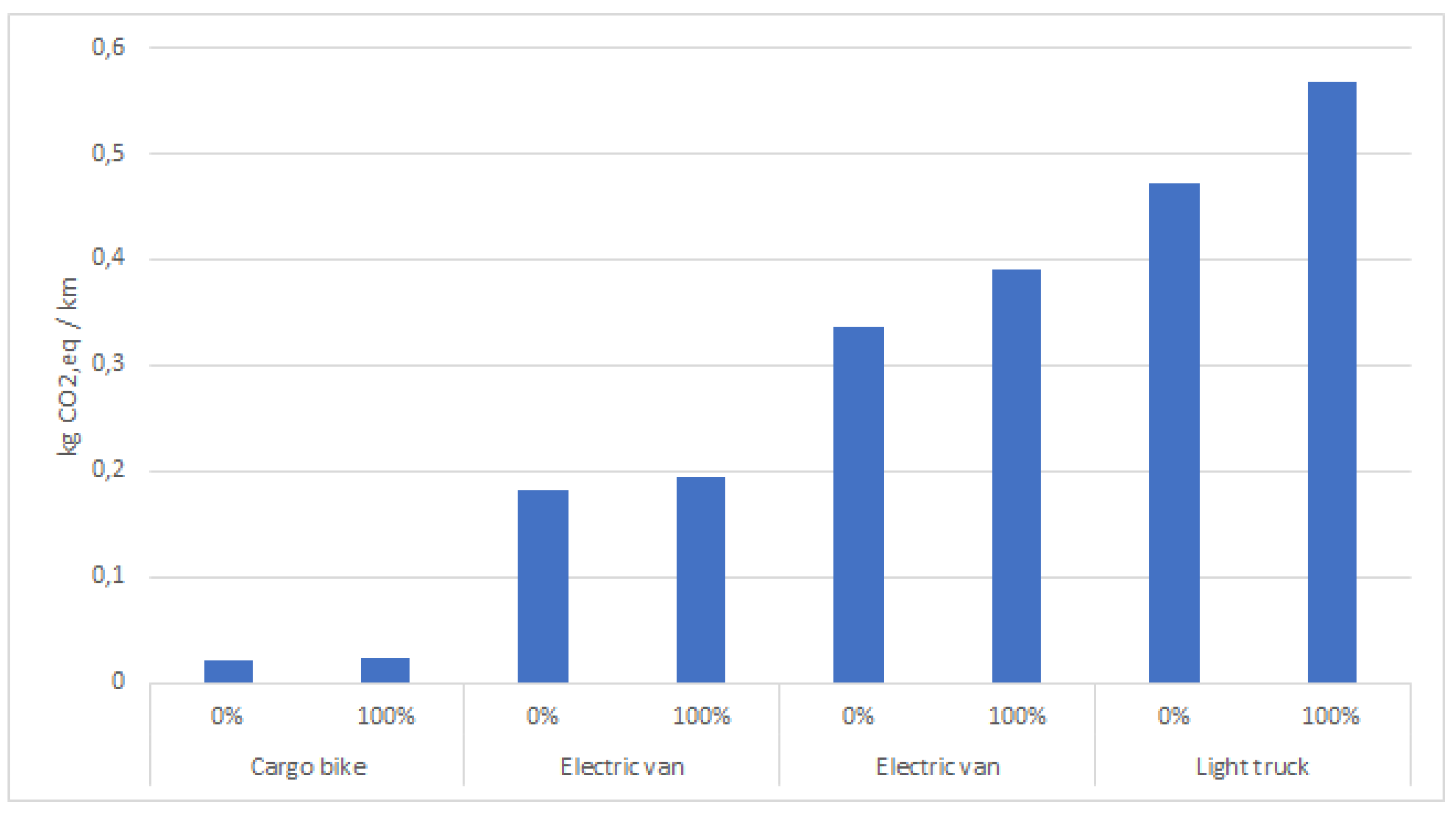
Two impact categories are assessed: GWP in and ozone formation (human health) in for all vehicles with a loading factor varying from 0% to 100%. The numerical results are presented in Table 1 and graphically displayed for the GWP category in Figure 1, where the results are shown in kg for each vehicle type, both empty (with a loading factor of 0%) and fully loaded (with a loading factor of 100%).
4.1.1. GWP
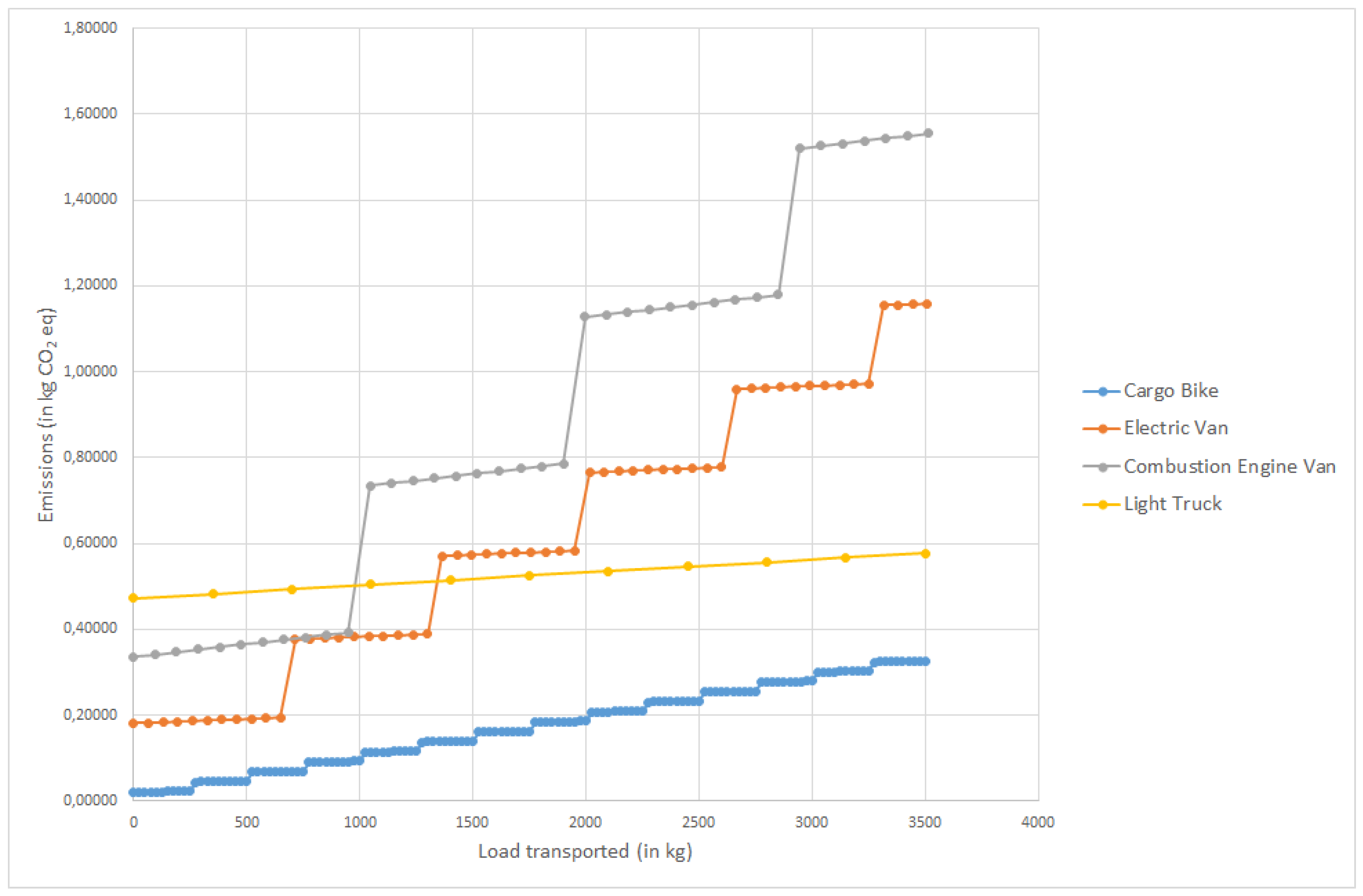
Figure 2 depicts the different emission levels for each type of vehicle, depending on transported load. It is assumed that one vehicle is loaded to 100% before engaging an additional vehicle. As this chart indicates, the cargo bike is the most ecological means of transport with the least environmental impact in terms of GWP. Within its constraints, it is always more advantageous to make delivery by cargo bike. However, it is the scope of activity in terms of distance (linked to battery life) and load capacity that limit the use of cargo bikes. According to the GWP factor, the electric van is the second most ecological option, up to a load of 1300 kg. Beyond that, the truck becomes more advantageous; it is, therefore, more ecological to take one truck rather than three electric vans. Similarly, it is more advantageous to use one truck rather than two combustion engine vans.
4.1.2. Ozone Formation
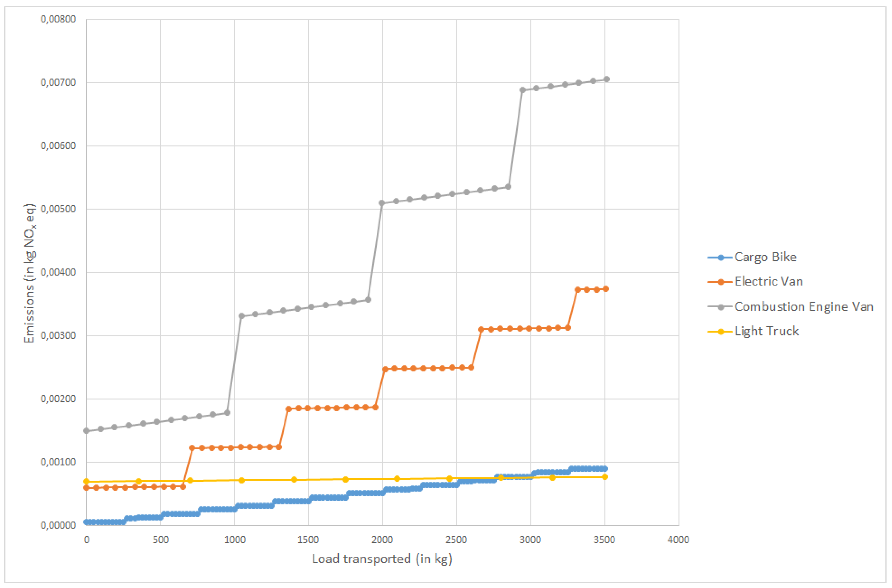
From the perspective of ozone formation, the ranking of means of transport is slightly different from that of the GWP factor. As it can be seen in Figure 3, a cargo bike is still the preferred mean of transport, but a truck loaded to 80% or more becomes more environmentally friendly than operating eleven cargo bikes. This can be explained by the fact that emissions have decreased by six times between the EURO 5 and EURO 6 trucks. Given this impact category, it is also more environmentally friendly to operate one truck rather than two electric vans. The combustion engine van represents the worst option in terms of emissions. A light truck is always more advantageous, independently of the load transported. Similarly, it is more advantageous to engage one truck instead of two combustion engine vans. As already mentioned, the combustion engine van used in the study is a EURO 5 van, as a EURO 6 combustion engine van is not available in the database.
4.2. Economic Aspects
Several papers discuss the financial aspect of urban delivery by cargo bike [43]. Amongst these, some point to the economic inefficiency of such a switch [44]. However, the results of these analyses should be updated. Indeed, electric cargo bikes are quite recent, and their technologies can improve in the future (especially in terms of battery autonomy). Furthermore, the purchase price has already decreased in recent years.
The results of the cost price assessment are displayed in Table 2 and Table 3. The daily operation seems to be the most economical for the cargo bike and the most expensive for the truck. However, the cargo bike travels an average of 50 km (compared to the truck that travels 160 km per day). By contrast, in terms of kilometres, the most economically advantageous transport option becomes the light truck; the cargo bike is the most expensive option.
5. Discussion
Several studies in various regions [45,46,47,48,49,50,51,52,53,54,55] show that the environmental impact of electric vehicles depends on how the electricity used by the vehicles is produced. The results may vary from country to country, depending on their respective electricity mix. The source of the electricity is not only used in activities directly related to transportation-to recharge the battery once down, but it is also used for the manufacturing of batteries or vehicles. The study in [51] analyses the variation of electric vehicle emissions depending on the electric power plant fleet and the efficiency during the use-phase. The authors show that some countries such as France or Norway are better-suited for electric vehicles adoption.
Therefore, the use of cleaner electricity such as renewable energy sources is essential to improve the environmental performance of electric vehicles. In [56], the author discusses the importance of electricity mix among European countries. He notably states that an electric vehicle using electricity produced from coal could emit more life cycle emissions than a conventional vehicle using petrol [57]. For instance, it is more environmentally friendly to implement delivery with electric vehicles in Sweden or France (where the electricity mix has a low carbon intensity) rather than in Poland or Germany (where the carbon intensity can be up to 60 times more intense) [58]. Therefore, a sensitivity analysis is carried out in Section 5.1 to compare selected European countries. Then, the cost price assessment is discussed in Section 5.2.
5.1. Electrical Mix Sensitivity Analysis
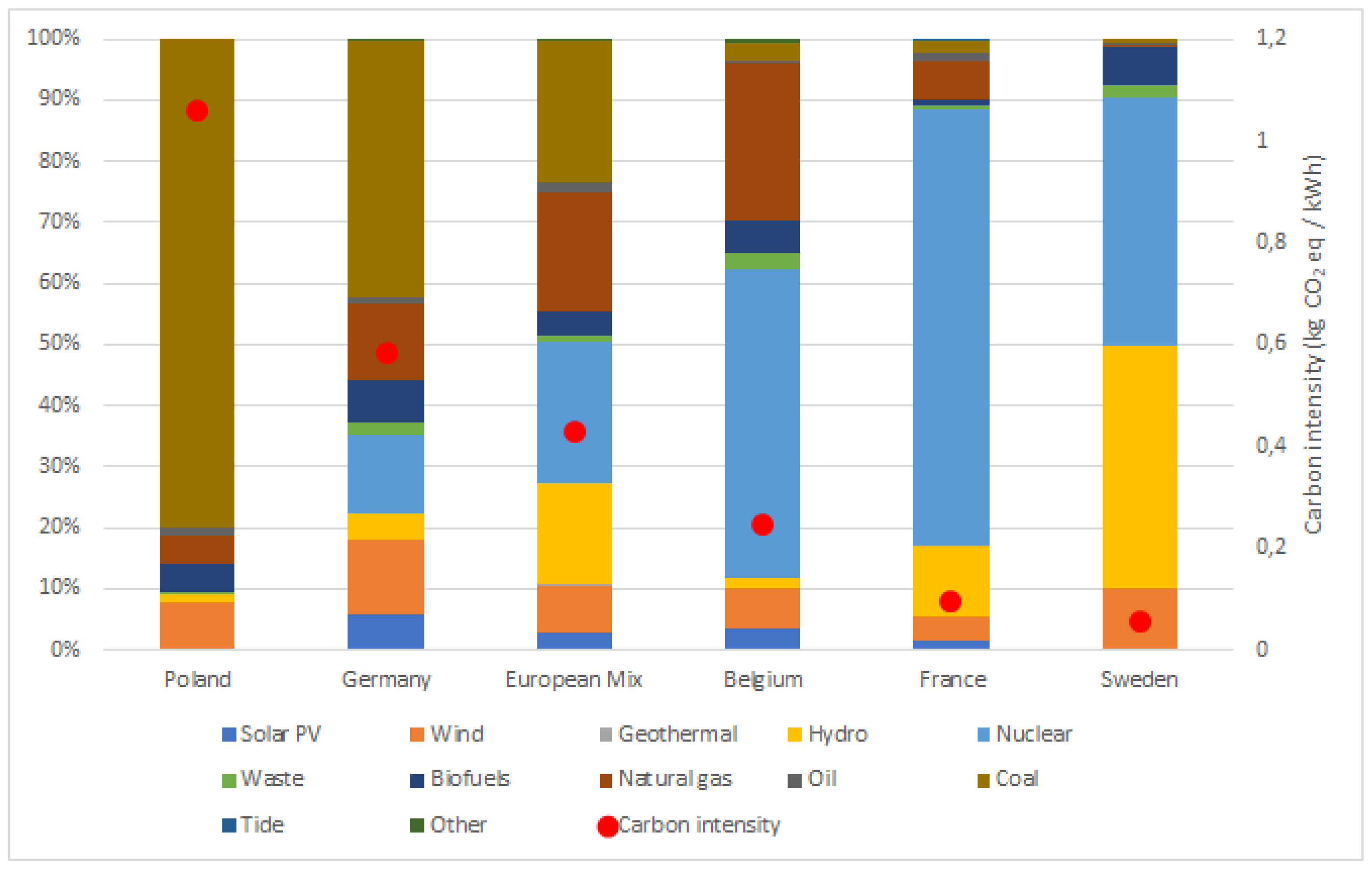
The regions chosen for this analysis are, in descending order of carbon intensity: Poland, Germany, European mix, Belgium, France, Sweden. Regarding the electricity mix in Figure 4, the share of each energy source in the electricity mix per country studied is depicted. In addition, the carbon intensity of each country is plotted above the electricity mix. Poland is unsurprisingly the country with the highest carbon intensity, as 80% of its electricity is produced by burning coal. Germany also has a high share of coal in its electricity mix (42%), placing it below the European average. Conversely, countries with a high share of renewable energy in their electricity mix have a lower carbon intensity. This is notably the case for Sweden, with 40% of its energy coming from hydroelectric sources. It should also be noted that nuclear power is a good alternative in terms of emissions, but has other disadvantages such as radioactive nuclear waste.
To understand where in the life cycle the greatest impacts of each vehicle come from, Figure 5 shows the relative share of each life cycle stage in the total emissions. Electric vehicles have no emissions during use. On the contrary, 70% of the emissions of combustion engine vehicles come from their operation, i.e., from the consumption of diesel or petrol during transport.
As shown in Figure 5, the impact of the electricity mix on internal combustion vehicles is minor, with the slight difference coming from the use of electricity to build and maintain the vehicle. Therefore, the sensitivity analysis is performed for the two electric vehicles, i.e., cargo bike and electric van. As the more a vehicle is loaded, the more it consumes and the more the impact of electricity has on the overall impact, both vehicles are estimated with a load factor of 50%. The respective electricity mix is derived from the Simapro software.
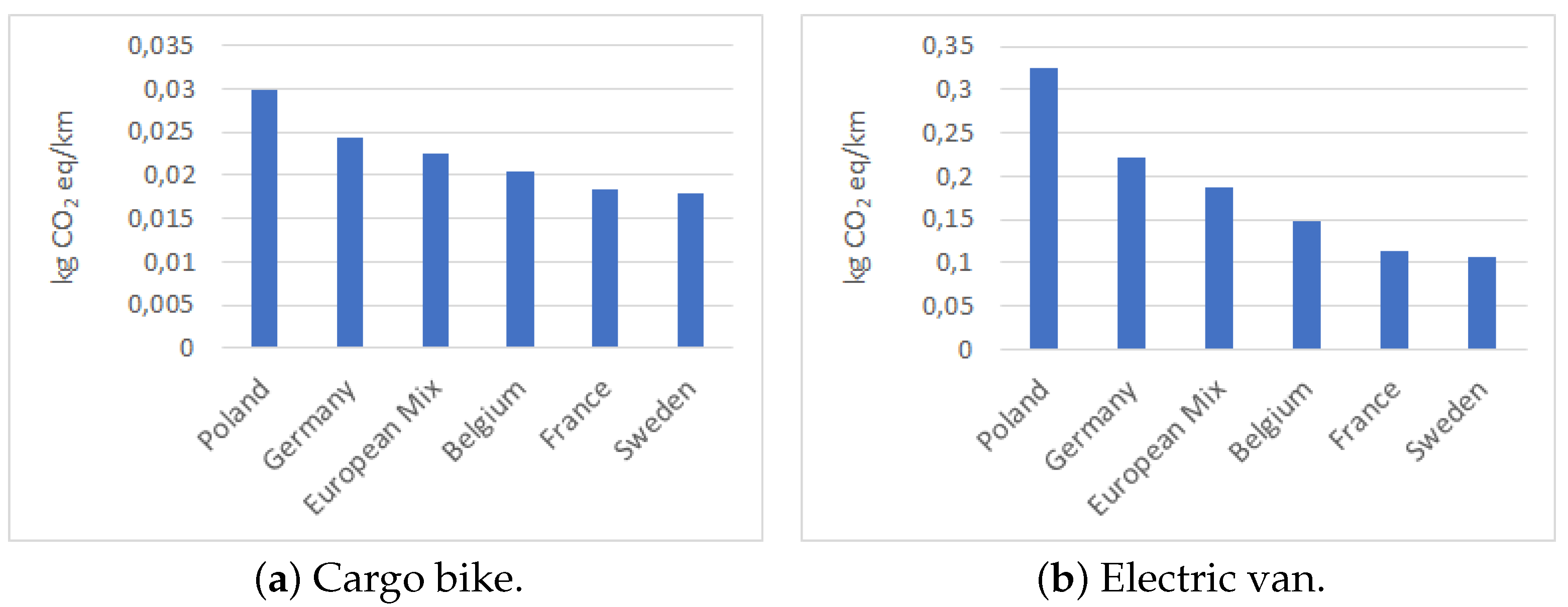
Looking at the results in Figure 6a, there is a 66% increase in kg of emissions between an electric cargo bike from Sweden and one from Poland. The difference is even more pronounced in the case of an electric van (Figure 6b), with emissions in Poland at 308% of those in Sweden. This is because the impact of electricity for the electric van is proportionately greater than for the cargo bike (Figure 5). Knowing this, an electric van in Poland becomes a less favourable solution than using a combustion engine van, as a combustion engine van emits slightly more and is able to carry a larger load.
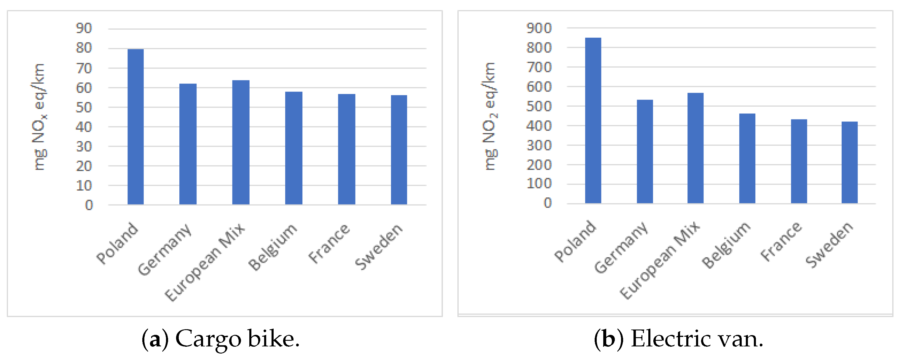
With respect to the emissions, the trend in these countries is the same but at a lower extent. Indeed, Figure 7a shows that the emissions of an electric cargo bike in Poland are 142% of those in Sweden; and, for an electric van (Figure 7b), emissions in Poland are 203% of those in Sweden. An electric van in Poland emits less than a combustion engine van.
In Poland and for some loads, it is possible that the vehicle with the lowest emissions (GWP) is different from the one with the lowest emissions (air quality pollutant through a health impact). Therefore, more precise parameters on the impacts of emissions should permit to evaluate the best trade-off between and . Indeed, premature mortalities due to degraded air quality are caused by population exposure to [59]. Thus, the impact increases with the population density of the geographical area where the transport takes place. In [60], the authors show the need to taken into account spatial patterns, regulations, socioeconomic characteristics, commercial structures, freight demand characteristics and distribution patterns when implementing city logistics measures to meet sustainability goals.
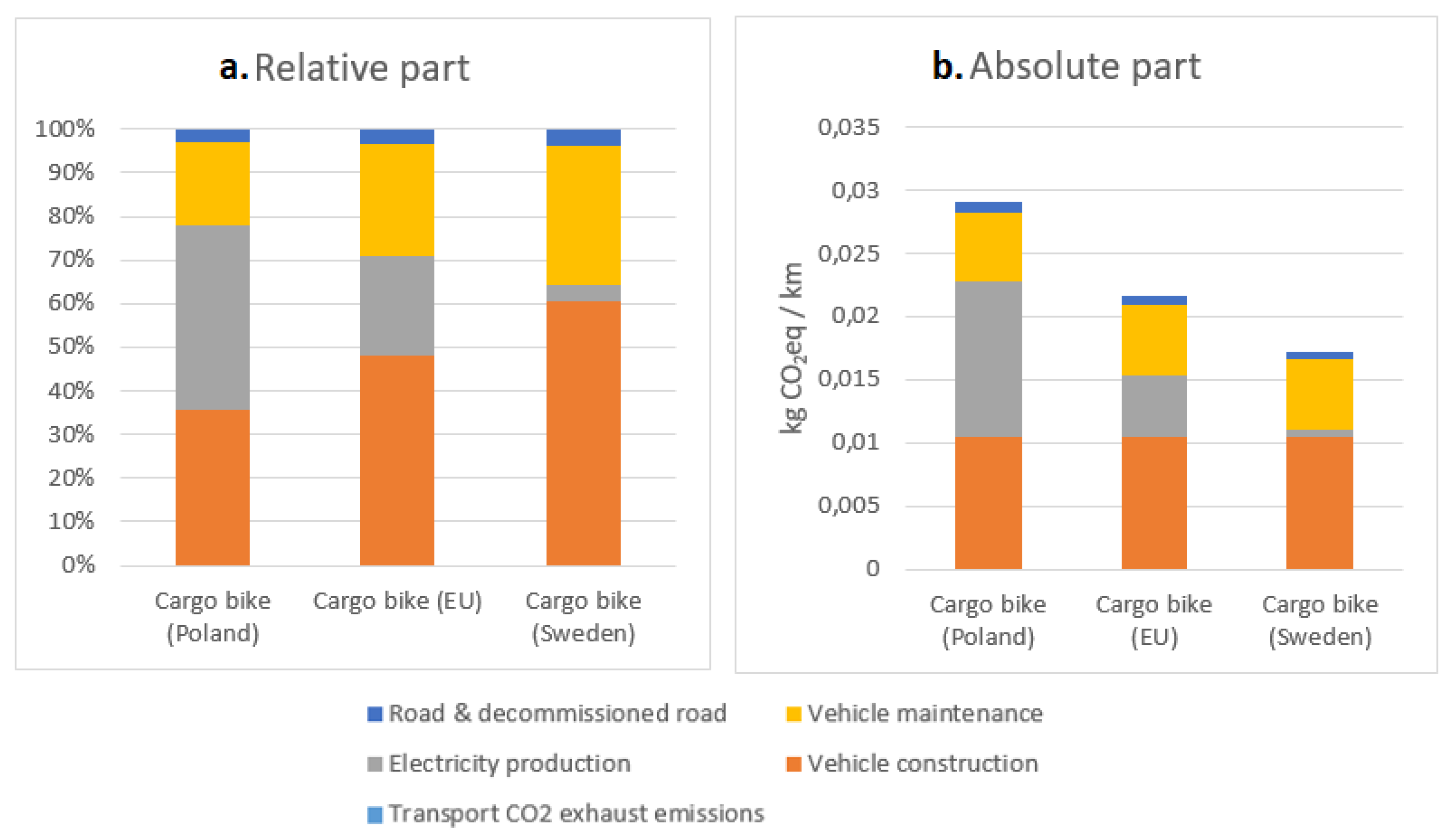
A closer look at the cargo bike shows the impact of the electricity mix on each emission category, especially on the electricity production category. The relative and absolute share of the impact of electricity production decreases for Sweden compared to Poland. The absolute share of the other categories remains similar in both countries, but consequently takes a larger relative share in Sweden. Indeed, as the impact of electricity production decreases, the impact of the other categories increases proportionally. On Figure 8b, it can be seen that the cargo bike running on Polish electricity has 66% more impact than the cargo bike running on Swedish electricity.
5.2. Cost Price Assessment Analysis
The parameters used are based on European averages. Still, it is interesting to note that prices widely vary according to the studied country. It can be, for instance, observed that Sweden is the most advantageous country for electric vehicles, both in terms of emissions and in terms of electricity price. Fuel and electricity prices also vary depending on the country. For instance (https://www.cnr.fr/prix-gazole-europe, accessed on 8 April 2021), the price of fuel is lowest in Bulgaria (with a rate of €0.842/l excluding VAT) and is highest in Sweden (€1.266/l excluding VAT). Whereas, electricity prices in the second half of 2020 were highest in Germany (€0.1818 per kWh) and Italy (€0.1514 per kWh). We observe the lowest prices in Sweden (€0.0588 per kWh) and Denmark (€0.0686 per kWh).
Depending on the country, tax benefits or purchase incentives may be offered for electric vehicles or less polluting vehicles. This would reduce the fixed cost of owning the vehicle in question.
The truck in our study is assumed to be a diesel vehicle since most trucks in Europe run on diesel, mainly because of the tax advantage. However, the tax advantage could be applied to petrol vehicles, which would impact on the emissions of heavy duty vehicles. A petrol truck would emit more , but less . Furthermore, according to the revised Renewable Energy Directive 2018/2001/EU [61], Member States must require fuel suppliers to supply a minimum of 14% of the energy consumed in road and rail transport by 2030 as renewable energy.
6. Conclusions
By comparing each mean of transport with the day’s use, the cargo bike is the most beneficial and least expensive solution. On the other hand, if we base the price on the number of kilometres travelled, the cargo bike becomes the most expensive solution. This makes sense given that the cargo bike travels on average three times less distance than the truck, for a daily cost that is only 23% lower than the truck. It can be concluded that the cargo bike is an interesting solution, both from an economic and ecological point of view, for deliveries characterised by a short distance to cover. Urban delivery is, therefore, particularly suitable. On the other hand, the transport of many parcels over a long distance will benefit from economies of scale by using a light truck.
As future research, it could be interesting to explore this aspect further to better appreciate the cases of applications where cargo bikes are economically advantageous. Sheth et al. [43] address this topic by developing a cost function model, including different parameters and variables such as distance between the depot and the customers, number of stops, distance between each stop and number of parcels per stop. This study concluded that the cargo bike is more cost-effective than a heavy vehicle for deliveries close to the depot (less than 10 km for an average of 4 stops per round), for which the population density is high and for a low delivery volume per stop.
Moreover, due to the uncertainty and variability of several parameters, it would be interesting to perform uncertainty analyses both for the environmental impacts and cost assessment, with uncertainty ranges such as in [51].
Author Contributions
Conceptualization, J.F., S.L.L. and L.V.; methodology, J.F., S.L.L. and L.V.; formal analysis, J.F., S.L.L. and L.V.; writing—review and editing, J.F., S.L.L. and L.V.; supervision, S.L.L.; funding acquisition, S.L.L. All authors have read and agreed to the published version of the manuscript.
Funding
This research was funded by the Walloon Region, grant number 8294, in the framework of the City Line project, supported by the cluster Logistics in Wallonia.
Institutional Review Board Statement
Not applicable.
Informed Consent Statement
Not applicable.
Acknowledgments
This publication presents the results of research carried out in the framework of the City Line project, Logistics in Wallonia. City Line is a collaborative logistics project supported by the Walloon region, aiming to promote urban delivery (and especially last mile delivery) via soft mobility such as cargo bikes. The authors thank the City Line partners for data sharing.
Conflicts of Interest
The authors declare no conflict of interest.
Appendix A

Table A1.
Parameters and assumptions made for the cost price analysis, for each vehicle type.
| Cargo Bike | Electric Van | Combustion Engine Van | Light Truck | |
|---|---|---|---|---|
| Operating conditions of the studied vehicle | ||||
| Average annual mileage (km) | 10.000 | 16.000 | 20.000 | 32.000 |
| Average daily mileage (km) | 50 | 80 | 100 | 160 |
| Number of operating days per year | 200 | 200 | 200 | 200 |
| Loading capacity (kg) | 250 | 650 | 950 | 3500 |
| Variable costs per kilometre of the studied vehicle | ||||
| Fuel/Electric consumption per 100 km (litre/kWh per 100 km, 50% LF) | 1.11 | 21.44 | 9.75 | 13.55 |
| Average price per litre of road fuel/electricity (€/l or €/kWh) | 0.1254 | 0.1254 | 1.04 | 1.04 |
| Price of a tyre | 30 | 80 | 80 | 300 |
| Life span of a tyre | 5000 | 41.500 | 41.500 | 120.000 |
| Annual expenditure on maintenance and repairs per vehicle (€) | 1000 | 2000 | 2000 | 6000 |
| Daily fixed costs of the studied vehicle | ||||
| Life span of the vehicle (years) | 2 | 9 | 11 | 17 |
| Value of the vehicle (€) | 4500 | 26.000 | 24.000 | 50.000 |
| Annual amount of insurance for a vehicle (€/year) | 100 | 500 | 500 | 1000 |
| Driver staffing costs for the operation of the vehicle | ||||
| Number of days a driver is working per year | 200 | 200 | 200 | 200 |
| Monthly service time (hours) | 136 | 136 | 136 | 136 |
| Monthly driving time (hours) | 50 | 50 | 50 | 50 |
| Number of days worked per month | 17 | 17 | 17 | 17 |
| Gross monthly salary (€/month) | 2700 | 3000 | 3000 | 3000 |
References
- European Commission. Sustainable and Smart Mobility Strategy–Putting European Transport on Track for the Futur. 2020. Available online: https://eur-lex.europa.eu/legal-content/EN/TXT/?uri=CELEX%3A52020DC0789 (accessed on 26 April 2021).
- European Commission. Transport Emissions-Climate Action-European Commission. 2017. Available online: https://ec.europa.eu/clima/policies/transport_en (accessed on 26 April 2021).
- Mellios, G.; Gouliarou, E. Greenhouse gas intensities of road transport fuels in the EU in 2018. Monitoring under the Fuel Quality Directive. Eur. Environ. Agency 2020. [Google Scholar] [CrossRef]
- Godínez-Zamora, G.; Victor-Gallardo, L.; Angulo-Paniagua, J.; Ramos, E.; Howells, M.; Usher, W.; De León, F.; Meza, A.; Quirós-Tortós, J. Decarbonising the transport and energy sectors: Technical feasibility and socioeconomic impacts in Costa Rica. Energy Strategy Rev. 2020, 32, 100573. [Google Scholar] [CrossRef]
- Marcucci, E.; Gatta, V.; Le Pira, M.; Elias, W. Modal Shift, Emission Reductions and Behavioral Change: Transport Policies and Innovations to Tackle Climate Change; Elsevier: Amsterdam, The Netherlands, 2019. [Google Scholar]
- Mostert, M.; Caris, A.; Limbourg, S. Road and intermodal transport performance: The impact of operational costs and air pollution external costs. Res. Transp. Bus. Manag. 2017, 23, 75–85. [Google Scholar] [CrossRef] [Green Version]
- Mostert, M.; Caris, A.; Limbourg, S. Intermodal network design: A three-mode bi-objective model applied to the case of Belgium. Flex. Serv. Manuf. J. 2018, 30, 397–420. [Google Scholar] [CrossRef] [Green Version]
- Tawfik, C.; Limbourg, S. Pricing problems in intermodal freight transport: Research overview and prospects. Sustainability 2018, 10, 3341. [Google Scholar] [CrossRef] [Green Version]
- Tawfik, C.; Limbourg, S. Scenario-based analysis for intermodal transport in the context of service network design models. Transp. Res. Interdiscip. Perspect. 2019, 2, 100036. [Google Scholar] [CrossRef]
- Li, L.; Zhang, X. Reducing CO2 emissions through pricing, planning, and subsidizing rail freight. Transp. Res. Part D Transp. Environ. 2020, 87, 102483. [Google Scholar] [CrossRef]
- Browne, M.; Allen, J.; Anderson, S. Low emission zones: The likely effects on the freight transport sector. Int. J. Logist. Res. Appl. 2005, 8, 269–281. [Google Scholar] [CrossRef]
- Ellison, R.B.; Greaves, S.P.; Hensher, D.A. Five years of London’s low emission zone: Effects on vehicle fleet composition and air quality. Transp. Res. Part D Transp. Environ. 2013, 23, 25–33. [Google Scholar] [CrossRef]
- Qadir, R.M.; Abbaszade, G.; Schnelle-Kreis, J.; Chow, J.C.; Zimmermann, R. Concentrations and source contributions of particulate organic matter before and after implementation of a low emission zone in Munich, Germany. Environ. Pollut. 2013, 175, 158–167. [Google Scholar] [CrossRef]
- Malina, C.; Scheffler, F. The impact of Low Emission Zones on particulate matter concentration and public health. Transp. Res. Part A Policy Pract. 2015, 77, 372–385. [Google Scholar] [CrossRef] [Green Version]
- Napoli, G.; Micari, S.; Dispenza, G.; Andaloro, L.; Antonucci, V.; Polimeni, A. Freight distribution with electric vehicles: A case study in Sicily. RES, infrastructures and vehicle routing. Transp. Eng. 2021, 3, 100047. [Google Scholar] [CrossRef]
- Wróblewski, P.; Drożdż, W.; Lewicki, W.; Dowejko, J. Total cost of ownership and its potential consequences for the development of the hydrogen fuel cell powered vehicle market in Poland. Energies 2021, 14, 2131. [Google Scholar] [CrossRef]
- Sælensminde, K. Cost–benefit analyses of walking and cycling track networks taking into account insecurity, health effects and external costs of motorized traffic. Transp. Res. Part A Policy Pract. 2004, 38, 593–606. [Google Scholar] [CrossRef]
- Bullock, C.; Brereton, F.; Bailey, S. The economic contribution of public bike-share to the sustainability and efficient functioning of cities. Sustain. Cities Soc. 2017, 28, 76–87. [Google Scholar] [CrossRef]
- Weiss, C.; Onnen-Weber, U. The challenge of sustainable last mile distribution of CEP services in small towns. Transp. Res. Procedia 2019, 39, 597–604. [Google Scholar] [CrossRef]
- CNR. Cost price repository Comité National Routier-CNR. 2021. Available online: http://www.cnr.fr/en/Indices-Statistics/Short-haul-rigids/Cost-price-repository (accessed on 8 April 2021).
- Knörr, W.; Seum, S.; Schmied, M.; Kutzner, F.; Anthes, R. Ecological transport information tool for worldwide transports. In Methodology and Data Update; IFEU Heidelberg, Oko-Institut: Heidelberg, Germany, 2019. [Google Scholar]
- Maibach, M.; Peter, M.; Sutter, D. Analysis of operating cost in the EU and the US. Annex 1 to Final Report of COMPETE Analysis of the contribution of transport policies to the competitiveness of the EU economy and comparison with the United States. Funded by European Commission-DG TREN. Karlsruhe, Alemanha. ISI/INFRAS/TIS/EE 2006. Available online: https://ec.europa.eu/ten/transport/studies/doc/compete/compete_annex_01_en.pdf (accessed on 13 August 2021).
- Bagieński, Z. Traffic air quality index. Sci. Total Environ. 2015, 505, 606–614. [Google Scholar] [CrossRef]
- Ziyadi, M.; Ozer, H.; Kang, S.; Al-Qadi, I.L. Vehicle energy consumption and an environmental impact calculation model for the transportation infrastructure systems. J. Clean. Prod. 2018, 174, 424–436. [Google Scholar] [CrossRef]
- ISO. ISO 14040:2006. 2021. Available online: https://www.iso.org/standard/37456.html (accessed on 26 April 2021).
- ISO. ISO 14044:2006. 2021. Available online: https://www.iso.org/standard/38498.html (accessed on 26 April 2021).
- Finnveden, G.; Hauschild, M.Z.; Ekvall, T.; Guinée, J.; Heijungs, R.; Hellweg, S.; Koehler, A.; Pennington, D.; Suh, S. Recent developments in life cycle assessment. J. Environ. Manag. 2009, 91, 1–21. [Google Scholar] [CrossRef]
- Goedkoop, M.; Heijungs, R.; Huijbregts, M.; De Schryver, A.; Struijs, J.; Van Zelm, R. A LCIA Method Which Comprises Harmonised Category Indicators at the Midpoint and the Endpoint Level_First Edition Characterisation| RIVM. 2013. Available online: https://www.rivm.nl/sites/default/files/2018-11/ReCiPe%202008_A%20lcia%20method%20which%20comprises%20harmonised%20category%20indicators%20at%20the%20midpoint%20and%20the%20endpoint%20level_First%20edition%20Characterisation.pdf (accessed on 26 April 2021).
- Spielmann, M.; Scholz, R. Life cycle inventories of transport services: Background data for freight transport (10 pp). Int. J. Life Cycle Assess. 2005, 10, 85–94. [Google Scholar] [CrossRef] [Green Version]
- Horvath, A. Environmental Assessment of Freight Transportation in the US. Int. J. Life Cycle Assess. 2006, 11, 229–239. [Google Scholar] [CrossRef]
- Facanha, C.; Horvath, A. Evaluation of life-cycle air emission factors of freight transportation. Environ. Sci. Technol. 2007, 41, 7138–7144. [Google Scholar] [CrossRef] [PubMed]
- Chester, M.; Horvath, A. Life-cycle assessment of high-speed rail: The case of California. Environ. Res. Lett. 2010, 5, 014003. [Google Scholar] [CrossRef]
- Van Lier, T.; Macharis, C. Assessing the environmental impact of inland waterway transport using a life-cycle assessment approach: The case of Flanders. Res. Transp. Bus. Manag. 2014, 12, 29–40. [Google Scholar] [CrossRef]
- Jones, H.; Moura, F.; Domingos, T. Life cycle assessment of high-speed rail: A case study in Portugal. Int. J. Life Cycle Assess. 2017, 22, 410–422. [Google Scholar] [CrossRef]
- Merchan, A.L.; Léonard, A.; Limbourg, S.; Mostert, M. Life cycle externalities versus external costs: The case of inland freight transport in Belgium. Transp. Res. Part D Transp. Environ. 2019, 67, 576–595. [Google Scholar] [CrossRef]
- Benveniste, G.; Rallo, H.; Canals Casals, L.; Merino, A.; Amante, B. Comparison of the state of Lithium-Sulphur and lithium-ion batteries applied to electromobility. J. Environ. Manag. 2018, 226, 1–12. [Google Scholar] [CrossRef] [PubMed] [Green Version]
- Bosch. eBike range calculator. 2021. Available online: https://www.bosch-ebike.com/en/service/range-assistant (accessed on 26 April 2021).
- Institut Paul Scherrer. Carculator: Etendue de l’analyse. 2021. Available online: https://carculator.psi.ch/ (accessed on 30 April 2021).
- Nissan. Nissan: e-NV200. Available online: https://www.nissan.fr/vehicules/neufs/e-nv200/caracteristiques-techniques.html (accessed on 3 March 2021).
- Lipasto. Van, Diesel, Gross Vehicle Mass 2,7t, Pay Load Capacity 1,2t - Delivery Driving. 2021. Available online: http://lipasto.vtt.fi/yksikkopaastot/tavaraliikennee/tieliikennee/padiesjakelue.htm (accessed on 3 April 2021).
- Lipasto. Delivery Lorry, Light-Gross Vehicle Mass 6t, Pay Load Capacity 3.5t-Delivery Driving. 2021. Available online: http://lipasto.vtt.fi/yksikkopaastot/tavaraliikennee/tieliikennee/kajakpienijakelue.htm (accessed on 3 April 2021).
- Eurostat. Electricity Price. 2020. Available online: https://ec.europa.eu/eurostat/statistics-explained/index.php?title=Electricity_price_statistics (accessed on 26 April 2021).
- Sheth, M.; Butrina, P.; Goodchild, A.; McCormack, E. Measuring delivery route cost trade-offs between electric-assist cargo bicycles and delivery trucks in dense urban areas. Eur. Transp. Res. Rev. 2019, 11. [Google Scholar] [CrossRef] [Green Version]
- Melo, S.; Baptista, P.; Costa, A. Comparing the Use of Small Sized Electric Vehicles with Diesel Vans on City Logistics. Procedia Soc. Behav. Sci. 2014, 111, 1265–1274. [Google Scholar] [CrossRef] [Green Version]
- Faria, R.; Marques, P.; Moura, P.; Freire, F.; Delgado, J.; de Almeida, A.T. Impact of the electricity mix and use profile in the life-cycle assessment of electric vehicles. Renew. Sustain. Energy Rev. 2013, 24, 271–287. [Google Scholar] [CrossRef]
- Bickert, S.; Kampker, A.; Greger, D. Developments of CO2-emissions and costs for small electric and combustion engine vehicles in Germany. Transp. Res. Part D Transp. Environ. 2015, 36, 138–151. [Google Scholar] [CrossRef]
- Huo, H.; Cai, H.; Zhang, Q.; Liu, F.; He, K. Life-cycle assessment of greenhouse gas and air emissions of electric vehicles: A comparison between China and the U.S. Atmos. Environ. 2015, 108, 107–116. [Google Scholar] [CrossRef]
- Nichols, B.G.; Kockelman, K.M.; Reiter, M. Air quality impacts of electric vehicle adoption in Texas. Transp. Res. Part D Transp. Environ. 2015, 34, 208–218. [Google Scholar] [CrossRef]
- Rangaraju, S.; De Vroey, L.; Messagie, M.; Mertens, J.; Van Mierlo, J. Impacts of electricity mix, charging profile, and driving behavior on the emissions performance of battery electric vehicles: A Belgian case study. Appl. Energy 2015, 148, 496–505. [Google Scholar] [CrossRef]
- Tamayao, M.A.M.; Michalek, J.J.; Hendrickson, C.; Azevedo, I.M.L. Regional Variability and Uncertainty of Electric Vehicle Life Cycle CO2 Emissions across the United States. Environ. Sci. Technol. 2015, 49, 8844–8855. [Google Scholar] [CrossRef]
- Canals Casals, L.; Martinez-Laserna, E.; Amante García, B.; Nieto, N. Sustainability analysis of the electric vehicle use in Europe for CO2 emissions reduction. J. Clean. Prod. 2016, 127, 425–437. [Google Scholar] [CrossRef]
- McLaren, J.; Miller, J.; O’Shaughnessy, E.; Wood, E.; Shapiro, E. CO2 emissions associated with electric vehicle charging: The impact of electricity generation mix, charging infrastructure availability and vehicle type. Electr. J. 2016, 29, 72–88. [Google Scholar] [CrossRef] [Green Version]
- Woo, J.; Choi, H.; Ahn, J. Well-to-wheel analysis of greenhouse gas emissions for electric vehicles based on electricity generation mix: A global perspective. Transp. Res. Part D Transp. Environ. 2017, 51, 340–350. [Google Scholar] [CrossRef]
- Choi, H.; Shin, J.; Woo, J. Effect of electricity generation mix on battery electric vehicle adoption and its environmental impact. Energy Policy 2018, 121, 13–24. [Google Scholar] [CrossRef]
- Rupp, M.; Handschuh, N.; Rieke, C.; Kuperjans, I. Contribution of country-specific electricity mix and charging time to environmental impact of battery electric vehicles: A case study of electric buses in Germany. Appl. Energy 2019, 237, 618–634. [Google Scholar] [CrossRef]
- Merchan, A.L. Importance of the Electricity Mix for Electric Vehicles to Help Obtain the SDGs. Ind. Innov. Infrastruct. Encycl. UN Sustain. Dev. Goals 2021. [Google Scholar] [CrossRef]
- European Environment Agency. Electric Vehicles in Europe. 2016. Available online: https://www.eea.europa.eu/publications/electric-vehicles-in-europe (accessed on 3 March 2021).
- European Environment Agency. CO2 Emissions Intensity. 2021. Available online: https://www.eea.europa.eu/data-and-maps/daviz/co2-emission-intensity-5 (accessed on 3 March 2021).
- Guerreiro, C. Air Quality in Europe: 2013 Report; Publications Office of the European Union: Copenhagen, Denmark, 2013; Available online: https://ketlib.lib.unipi.gr/xmlui/handle/ket/1037 (accessed on 13 August 2021).
- Nuzzolo, A.; Comi, A.; Ibeas, A.; Moura, J.L. Urban freight transport and city logistics policies: Indications from Rome, Barcelona, and Santander. Int. J. Sustain. Transp. 2016, 10, 552–566. [Google Scholar] [CrossRef]
- Renewable Energy–Recast to 2030 (RED II)-EU Science Hub- European Commission. 2019. Available online: https://ec.europa.eu/jrc/en/jec/renewable-energy-recast-2030-red-ii (accessed on 16 July 2021).
Figure 1.
Comparison of the impacts (GWP) of different means of transport in km, according to the loading factor.
Figure 1.
Comparison of the impacts (GWP) of different means of transport in km, according to the loading factor.

Figure 2.
Emissions of for each type of vehicle.

Figure 3.
Emissions of for each type of vehicle.

Figure 4.
Electricity mix per country Source: https://www.iea.org/regions/europe, accessed on 26 April 2021 (2016 data).
Figure 4.
Electricity mix per country Source: https://www.iea.org/regions/europe, accessed on 26 April 2021 (2016 data).

Figure 5.
Life-cycle emissions for different vehicles (in proportion).

Figure 6.
Emissions of according to the electric mix.

Figure 7.
Emissions of according to the electric mix.

Figure 8.
Life-cycle emissions for cargo bikes from (1) Poland, (2) Europe and (3) Sweden. (a) Relative part. (b) Absolute part.
Figure 8.
Life-cycle emissions for cargo bikes from (1) Poland, (2) Europe and (3) Sweden. (a) Relative part. (b) Absolute part.

Table 1.
Emissions depending on the loading factor.
| Vehicle Type | Electric Cargo | Electric Van | Combustion | Light Truck | ||||
|---|---|---|---|---|---|---|---|---|
| Bike | Engine Van | |||||||
| Loading factor (%) | 0 | 100 | 0 | 100 | 0 | 100 | 0 | 100 |
| GWP () | 20.7 | 23.6 | 181.5 | 193.8 | 336.0 | 389.0 | 472.7 | 567.4 |
| Ozone formation, Human health () | 0.061 | 0.066 | 0.555 | 0.578 | 1.535 | 1.794 | 0.685 | 0.771 |
Table 2.
Trinomial formula and annual cost price.
| Cargo Bike | Electric Van | Combustion Engine Van | Light Truck | |
|---|---|---|---|---|
| Kilometre term (€/km) | ||||
| Hourly term (€/hour) | ||||
| Daily term (€/day) | ||||
| Annual cost (€) | 46,894 | 53,412 | 56,352 | 62,770 |
Table 3.
Cost price for each vehicle type.
| Cargo Bike | Electric Van | Combustion Engine Van | Light Truck | |
|---|---|---|---|---|
| The day of use | ||||
| The hour of driving | ||||
| Driver’s duty hour | ||||
| Kilometre driven | ||||
| Loaded kilometre | ||||
| Unit kilograms × km driven | ||||
| Unit kilograms × loaded km |
Publisher’s Note: MDPI stays neutral with regard to jurisdictional claims in published maps and institutional affiliations. |
© 2021 by the authors. Licensee MDPI, Basel, Switzerland. This article is an open access article distributed under the terms and conditions of the Creative Commons Attribution (CC BY) license (https://creativecommons.org/licenses/by/4.0/).
Share and Cite
MDPI and ACS Style
Fraselle, J.; Limbourg, S.L.; Vidal, L. Cost and Environmental Impacts of a Mixed Fleet of Vehicles. Sustainability 2021, 13, 9413. https://0-doi-org.brum.beds.ac.uk/10.3390/su13169413
AMA Style
Fraselle J, Limbourg SL, Vidal L. Cost and Environmental Impacts of a Mixed Fleet of Vehicles. Sustainability. 2021; 13(16):9413. https://0-doi-org.brum.beds.ac.uk/10.3390/su13169413
Chicago/Turabian StyleFraselle, Justin, Sabine Louise Limbourg, and Laura Vidal. 2021. "Cost and Environmental Impacts of a Mixed Fleet of Vehicles" Sustainability 13, no. 16: 9413. https://0-doi-org.brum.beds.ac.uk/10.3390/su13169413
Note that from the first issue of 2016, this journal uses article numbers instead of page numbers. See further details here.