
Health-Related Benefits of Different Indoor Plant Species in a School Setting


Research Unit of Ecological Building Technologies, Institute of Material Technology, Building Physics and Building Ecology, Faculty of Civil Engineering, Vienna University of Technology, Karlsplatz 13/207-3, A-1040 Vienna, Austria
*
Author to whom correspondence should be addressed.
Sustainability 2021, 13(17), 9566; https://0-doi-org.brum.beds.ac.uk/10.3390/su13179566
Submission received: 3 May 2021
/
Revised: 23 July 2021
/
Accepted: 29 July 2021
/
Published: 25 August 2021
(This article belongs to the Collection Urban Green Infrastructure for Climate-Proof and Healthy Cities)
Abstract
:Humans spend more than 80% of their lives indoors resulting in an increased demand for high indoor air quality (IAQ). At the same time, indoor air tends to be at least twice as polluted as outdoor air, and health threats caused by long-term exposure to indoor air pollution are rising. Few experiments under real-life conditions have demonstrated positive effects of indoor plants on parameters related to IAQ, resulting in improved humidity and temperature, reduced particulate matter concentration and CO2 levels. Indoor living walls allow the presence of many plants—without taking up valuable floor area. This article presents the results of conducted measurements on four do-it-yourself green walls planted with different plant species that are typically used for vertical indoor greenery (golden pothos, Boston fern, spider plant and a combination of plants) in a school setting. Besides the parameters of air humidity and temperature, CO2, mold spore and particulate matter levels, influences on room acoustics were investigated. Based on a custom-developed evaluation matrix, the plants were compared with each other and a reference without plants. The results show that no species led to deterioration of IAQ. Golden pothos had the most substantial effect and delivered improvements in all examined parameters.
1. Introduction
People in present-day society spend 80% to 90% of their time indoors [1]. Hence, living in a healthy indoor environment with satisfying indoor air quality (IAQ) is of vital importance, as suggested by the increasing occurrence of sick building syndrome (SBS) [2]. Between 80% (developed countries) and 90% (EU-28) of the average 250 million liters of air a person breathes in the course of their life (about 10,000 L per day) is sourced from indoors (houses, workplaces, schools, shopping centers, public buildings or means of transport) [3]. The USA Human Activity Pattern Survey similarly disclosed that an average adult spends 86% of their time indoors and an additional 6% inside public transport or private vehicles [4].
Climate change, increasing urbanization and densification in inner-city areas require new ways and approaches to increase the quality of life and living comfort, especially when it comes to school buildings, where young people spend most of their time together in one room with many other students. Urban and indoor green infrastructure has the potential to contribute to a solution by providing removal of pollutants and other effects, which has been proven in numerous international studies such as [5,6]. The indoor concentration of air pollutants might be higher than the outdoor concentration of air pollutants if the outdoor-sourced contaminated air enters indoor occupied spaces and combines with indoor-sourced pollutants [7]. For the most part, in highly industrialized or traffic-dense areas, indoor air pollution has not been acknowledged as outdoor air pollution has been. Yet, the health threats of indoor air pollutants caused by long-term exposure have become more evident over the last decades as buildings are progressively sealed against the outside climate conditions to obtain cooling and heating energy cost savings [8].
At a global level, the World Health Organization (WHO) estimated that every year approximately 3.8 million people die from illnesses related to indoor air pollution, mainly due to cooking or heating, which is around 7.7% of the worldwide mortality [9]. Accordingly, the assessment of indoor air pollution is becoming more important due to its direct influence on human health. As stated in [10], about 25% of US citizens are suffering from poor IAQ during their everyday obligations. Further, IAQ was classified as a priority concern for children’s health [8] and one of the USA’s largest environmental threats [10]. Health problems such as respiratory illnesses, allergies and even cancerous diseases associated with indoor air pollution and IAQ are intensified by SBS [11]. In addition to health influence, poor IAQ reduces workplace productivity by 10–15% [12].
Indoor air pollutants, which contribute to bad IAQ, include particulate matter, bioaerosols and over 400 different chemical compounds, mainly volatile organic compounds (VOCs), for instance, formaldehyde, benzene, toluene, ethylbenzene and xylene (BTEX) and trichloroethylene, and inorganic compounds (VICs) such as carbon monoxide (CO), carbon dioxide (CO2), nitrogen oxides (NOx) and ozone (O3). Additionally, pollutant sources and emission rates may rapidly change over time [13]. Indoor pollutant sources include permanent sources (building materials, carpets, paints, varnishes, etc.) and occasional sources (furniture, cleaning and disinfection products, cooking, personal care products, tobacco smoke, etc.), while outdoor pollutant intrusion mostly depends on road traffic and industry [14].
Health issues caused by exceedingly increased concentration of CO2 are irritation and dryness of mucous membranes, fatigue and headache. In the middle of the 19th century, Pettenkofer defined a guideline value for the maximum CO2 concentration in living rooms and lounges with a value of 0.1 vol% CO2 (1000 ppm), the so-called “Pettenkofer number”, which is used as the basis for calculations and regulations, especially in the area of ventilation and air-conditioning systems. In Austria, according to the “Grenzwerteverordnung (2011)”, the maximum valid CO2 level is 5000 ppm (9000 mg/m3) or 10,000 ppm (18,000 mg/m3) in an assessment period of 60 min [15].
In addition to the measurement of selected indoor air pollution, the temperature and climatic conditions are also the focus of investigations. Especially humidity plays a very important role. The occurrence of the following health effects in working spaces is associated with too low humidity: Drying of mucous membranes, colds, eye complaints, skin complaints and electrostatic charging and discharging [16,17]. Studies on the influence of relative humidity on the development of diseases were already conducted in the 1960s [18]. In this context, a connection between the survival of pathogens and relative humidity was established. Diseases or irritations of the skin, eyes and upper respiratory tract are often associated with low relative humidity indoors during the winter season [17,19]. Dry and cold air favors infections of the upper respiratory tract such as colds and throat infections in particular [20,21]. This is most likely due to the higher stability of virus particles at low humidity and low temperatures which has already been shown for rhinoviruses [22], influenza A viruses [23] and numerous others [22]. However, not only low but also immensely high air humidity has an important effect on human health, especially when combined with high temperature. This combination can lead to discomfort or to heat stroke, exhaustion and even possibly death. Furthermore, it can affect allergies and aggravate diseases in the respiratory system caused by specific biological agents (mites and mildew) [24]. Both passive and active ventilation can help extract pollutants and moisture from indoor spaces and provide residents with a more comfortable and healthier environment. Present-day buildings are built in such a manner that leakage is reduced. This, however, leads to an increased potential for listed illnesses [25]. On the other hand, the presence of nature is considered advantageous in terms of both mental and physical health [26]. Therefore, it is common for people to grow indoor plants in order to improve their overall wellbeing [27]. Moreover, observations have shown that indoor plants have a positive impact on general wellbeing [28,29]. Recently, a study conducted on three buildings located in Vienna, Austria, with six greened and three reference rooms without greenery, has shown that even when only considering the influence on air humidity, the number of sick leave days per office worker can be decreased. Furthermore, the calculations and analyses have shown that, assuming the mentioned reduction in sick leave, the greenery with standard specifications will be profitable after about 4.5 years [30]. The research was carried out following a previous project which, in a classroom greened by a living wall system that took only about 1% of classroom volume, showed that even in these seemingly negligible proportions, an effect on the indoor climate and IAQ was observable. Furthermore, it showed that the relative air humidity in the greened classroom was higher than in the not greened classroom, which causes a higher comfort level in winter months [31].
Early studies have displayed the significance of potted plants’ contribution to air cleansing through their foliage [32]. On the contrary, Godish and Guindon [33] discovered in a lab experiment that the highest air filtration occurs while using defoliated plants. That led them to the conclusion that air filtration might be associated with soil medium factors. Fjeld and Bonnevie [34] stated that plants, alongside roots and microorganisms occupying the root zone, create an ecosystem that may function as an air-purifying system. In addition to that, during the process of photosynthesis, plants release oxygen and consume carbon dioxide. As a result, this might lead to reduced ventilation demand and therefore contribute to a decrease in energy consumption. Scientific research since 1989 has disclosed the significance of plant influence on urban air pollution reduction [35,36,37,38,39,40,41]. However, an insufficient amount of research examining indoor plants’ effects on IAQ, humidity and temperature has been based on experiments performed in a daily-living environment. Knowles et al. [42] showed that indoor plants could remove more than 80% of indoor contaminants. Field measurements by Tarran et al. [43], performed on 60 office buildings, confirmed that indoor plants could decrease the total volatile organic compound (TVOC) amount in an indoor environment down to 25%. Pennisi and van Iersel [44] conducted an experiment in order to define the decrease of carbon dioxide amount associated with the use of various indoor plant species. This led to the conclusion that smaller plant species have a worse ability to consume CO2 quantities compared to larger plant species.
Furthermore, a living wall system is also able to serve as acoustic insulation [45]. Studies show that sound levels can be reduced due to vegetation in three possible ways. The first mechanism is the reflection and dispersion of sound by plant elements, including leaves, branches and trunks. Secondly, sound can be absorbed by vegetation itself. This happens due to plants’ mechanical vibrations which are caused by sound waves. Lastly, the growth media cause destructive interference of sound waves, resulting in a reduction of sound levels [46,47]. Hence, there are diverse factors influencing noise reaction in a green-wall system, including materials used as components of structure, growth medium and the overall coverage of foliage and substrate.
The positive effects of indoor greening on human health, especially in urban environments where air quality is usually poorer due to increased sources of pollution, have already been demonstrated. The requirements for IAQ in learning and teaching spaces for pupils of a young age are particularly high so that children and adolescents can grow up in spaces with the healthiest and highest possible quality, as already shown in [48]. Especially for children growing up in the city, plants in the classroom enable them to discover and foster a relationship with nature. Studies of vertical indoor greening as a space-saving green infrastructure in classrooms have not yet been investigated in terms of their impact on IAQ under real-life conditions. Vertical greenery in classrooms, which has been installed so far, is always equipped with a mixture of plants. The plants are selected on the basis of their suitability for use in wall greening and their robustness for use in a school so that students can also take over parts of the care and possibly also propagate the plants as part of the lessons, for example. However, in the past, the selection process has not yet considered which plants perform best in terms of pollutant removal and thus contribute most to better indoor air and better learning and teaching conditions. In this article, the influence of three different plant species—golden pothos (Epipremnum aureum), Boston fern (Nephrolepis exalta) and spider plant (Chlorophytum comosum)—as well as a combination of plants typically used in indoor living walls, planted in do-it-yourself (DIY) green walls on selected parameters were examined. Since, in addition to hygrothermal comfort and pollutant concentrations, room acoustics also contribute to high learning environment quality, the study additionally observed the effect of these plant species in combination with the DIY green wall construction on room acoustics, analyzing their influence on reverberation time and sound absorption. Furthermore, the mold spore concentration in the same room was measured to make sure that no exposure of spores was caused by the living walls.
Everyday life in classrooms is very dynamic, and highlighting the differences of certain measures under real conditions is only possible if as many uncertainties as possible can be cleared up in advance or if optimizations have been carried out in advance. When considering wall greening, plant selection is an extremely important aspect, which has not yet been given any attention in terms of its influence on IAQ, pollutant concentrations and in practice. This research focused on highlighting the differences of variously planted green walls in classrooms as a measure to improve the learning environment. The aim of this experimental study presented was to investigate whether the selected different plants have a measurable effect on selected parameters regarding IAQ, as well as room acoustics with the goal of subsequently being able to make a statement regarding which of the plants should be used for the greatest possible improvement of IAQ in classrooms to create a high-quality learning environment for students. Based on the results from the present research, further long-term studies can then follow to analyze the locally measured impacts for their relevance to the IAQ of the entire area.
2. Materials and Methods
2.1. Green Infrastructure
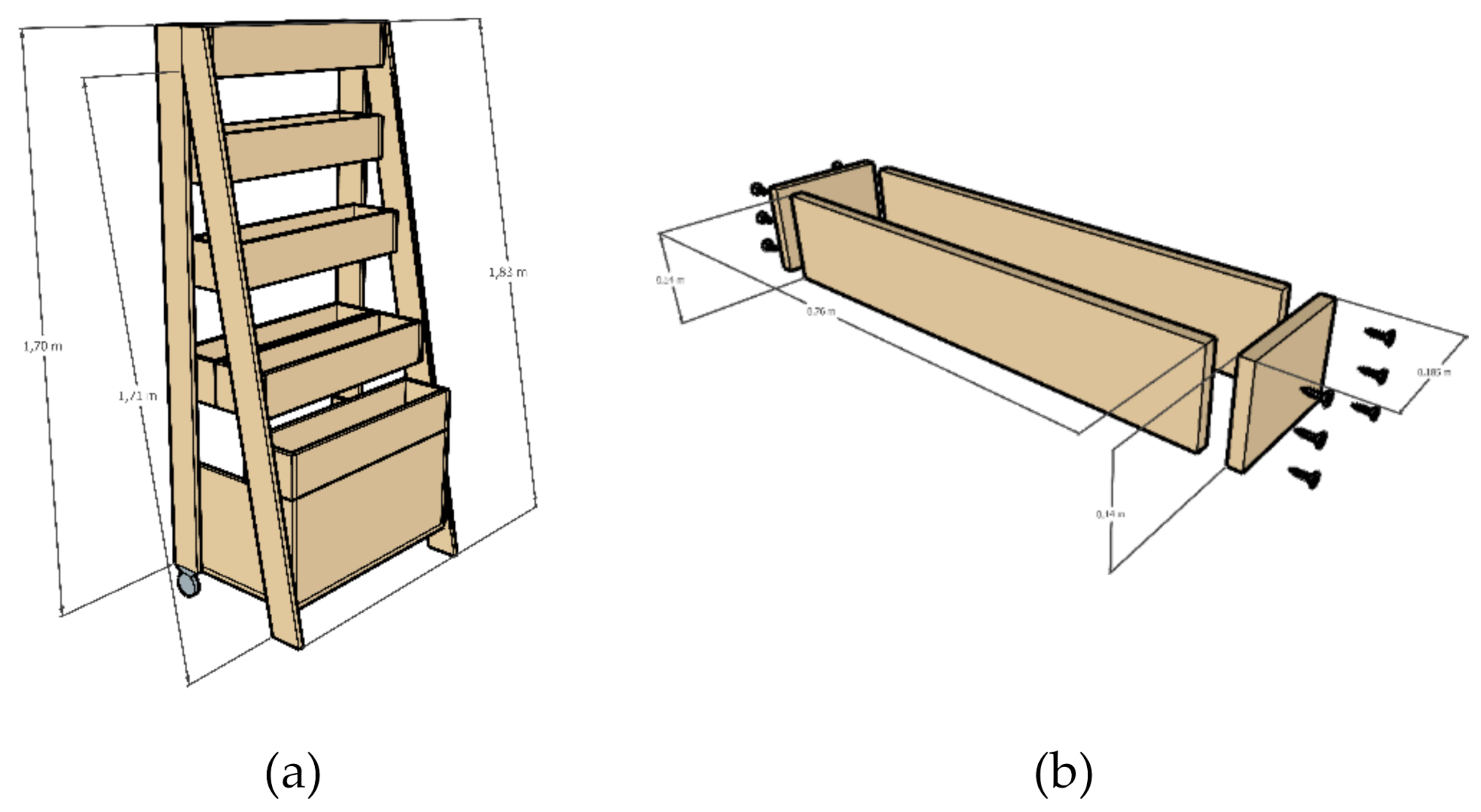
In the scope of the research, the green infrastructure used were DIY green walls that were constructed with students and were already developed as a part of a previous research project [49]. For the purpose of this study, four DIY green walls were built, and the selected plants were positioned. A mineral substrate based on natural zeolites, sold under the name “Zeobon® Zeostrat® 2/8”, was used as the substrate. Figure 1 shows the design of the DIY green walls during the planning phase.
The selection criteria of used plant species included the influence of the plant species on room climate, the potential ability to extract particulate matter particles and other air pollutants, and the suitability for use in an automatically irrigated greening system based on zeolite substrate. Table 1 shows the selected plants for the DIY green walls. In order to achieve a comparison of different forms of vegetation, plants with different morphology were selected, and it was ensured that at the beginning of the measurements, all plants in use were of the same relative size and therefore presented similar leaf mass. In the course of the project, the leaf mass was not further influenced by any means, which implies that different growth rates had influence on the results. Table 2 and Table 3 show rough estimations of the expected CO2 and particulate matter removal rates per single potted plant. Due to lack of sufficient data and comparability between different studies, absolute values are not relevant and only the ranking of the plant species is meaningful. In this experiment, each DIY green wall consisted of ~25 plants, thus, for example, leading to an expected CO2 removal of ~2000 ppm per hour for golden pothos. However, since the experiments were conducted under real-life circumstances and undefined amounts of CO2 and particulate matter were brought into the used rooms during measurements, a comparison between the created results and the estimations was not possible.
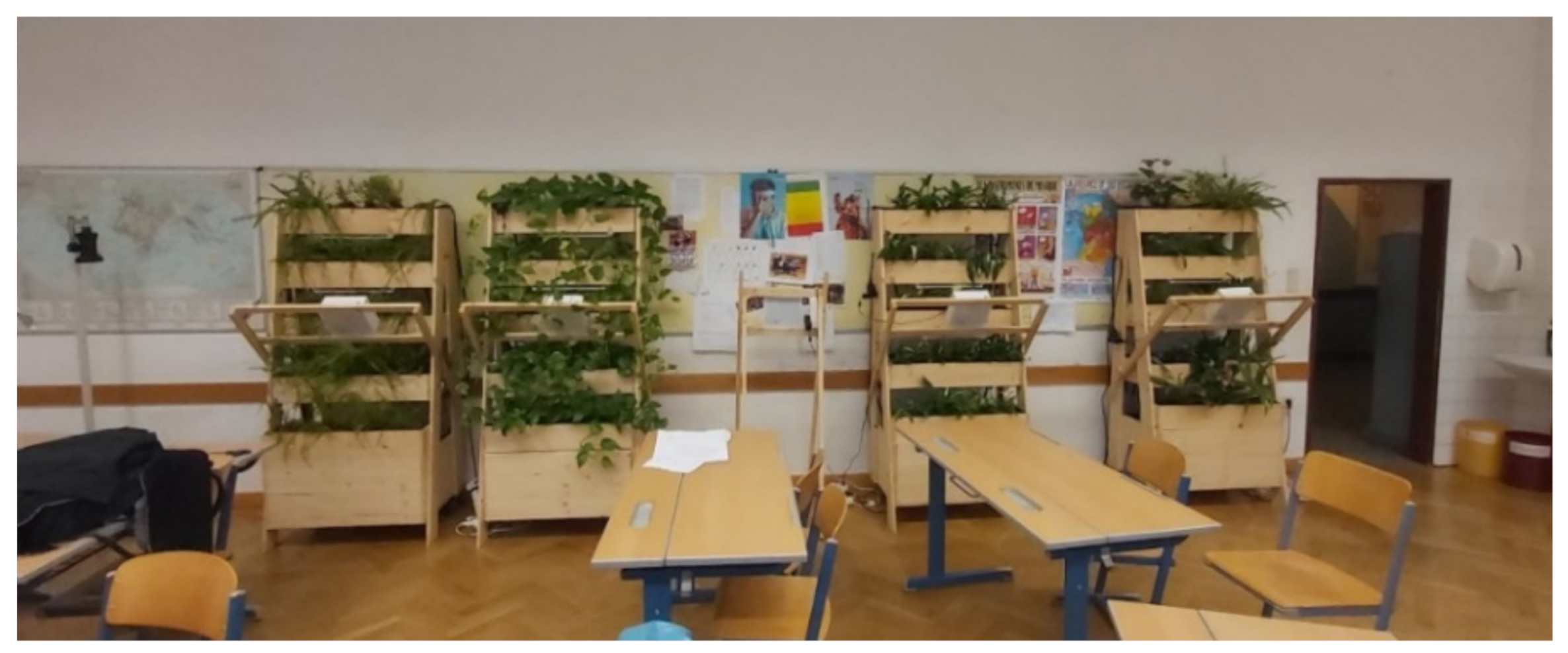
In order to ensure healthy growth and vital appearance, the plants were regularly supplied with water from a 70 L tank via a pump for automatic irrigation through adjustable drippers. In addition, fertilizer for green plants was added manually at regular intervals using a watering can. The watering intervals were adjusted in the course of the project according to the observed needs of the individual plant species. Figure 2 shows the DIY green walls with the respective plant species in week 13 2020.
To supply additional light to the plants, lamps (brand: MCIX) with a power consumption of 60 W, divided into 5 LED strips, were installed above the individual troughs. Throughout the duration of the project, it soon turned out that the plant lamps, due to the short distance to the plants and the simultaneous generation of heat, led to damage of the plants and were removed accordingly. As a result, the influence of lamps was not investigated. During the course of the experiment, it was observed that golden pothos, followed by the combination of plants and Boston fern, showed the least sensitivity to external influences such as under- or overwatering. Golden pothos and Boston fern showed general robustness with close to no losses due to withering. On the other hand, the advantage of the combination of plants was the fact that if any problems occurred, only specific plant species, such as spider plant, withered. Furthermore, all specimens of spider plant had to be exchanged with peace lily after all measurements were accomplished because significant losses due to withering were observed repeatedly and specimens of spider plant had to be replaced weekly.
2.2. Measuring Devices
For air quality measurements, devices, developed and sold under the name “AirSensEUR”, were installed. Mentioned devices are part of an open-source project, partially funded by the European Union. In [45], a detailed guide about the setup and use, aswell as schematics and diagrams can be found. These devices, from now on referred to as “Air Quality Monitoring Devices (AQMDs)”, were selected primarily because of their open architecture and comparatively inexpensive purchase. In comparison to traditional measuring devices, devices such as this offer the possibility of installing a dense network of sensors at various points for an extended period of time, without taking up a lot of space. For comparative measurements of particulate matter concentrations, such as those carried out in this project, however, the correlation of the individual sensors to one another or to a series of measurements at a reference measuring point with high accuracy must be determined and the measured values must be adjusted accordingly. Table 4 shows the individual utilized sensors of the “AQMDs” with the respective sensor name, the associated measurements carried out and the accuracy according to the manufacturer.
To determine the local effects of the various plant species on parameters of IAQ, AQMDs were installed at a distance of approx. 20 cm to the planted troughs, as shown in Figure 3. In addition, a fifth measuring device on a non-planted construction at the same height, as shown in Figure 3 and Figure 4, was used as a reference to get an indication of the local IAQ without influence of a green wall. The aim of the research carried out was to highlight the differences between the plants used and to show if plants are capable of reducing the total pollutant concentration without considering concrete exposure scenarios that would affect users. The location for the measuring devices was therefore chosen on the DIY green walls in direct proximity to the plants. Since measurements close to the green walls are hardly representative of all the air in the corresponding room, mean values were used to calculate the results so that airflow also had influence on the presented values. Further investigation on the present airflow was not executed because of the limitations that came with measuring in a frequently used classroom and limited time constraints.
To begin with, the DIY green walls were placed together in a rarely used corridor, on the one hand, to give the plants time to get used to the conditions and, on the other hand, to determine to what extent the exact location in a room influences the measurements. It was found that the proximity to radiators and passageways, or open doors, in particular, interfered with the measurements. In order to be able to compare the plant species, it was decided to place the DIY green walls together in a larger classroom during the measuring period. This ensured that influences affecting the entire room (ventilation, type and time of use) were more likely to be eliminated and results could be compared. The door of the class was mostly kept closed and was only opened during breaks. Table 5 gives an overview of locations and corresponding time periods of the green walls during the examination.
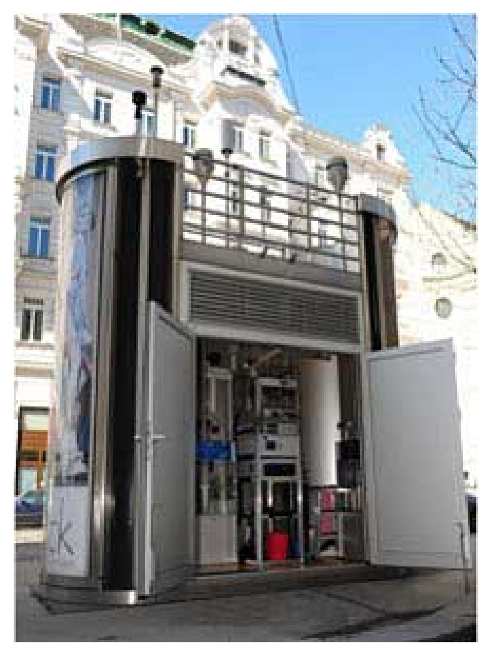
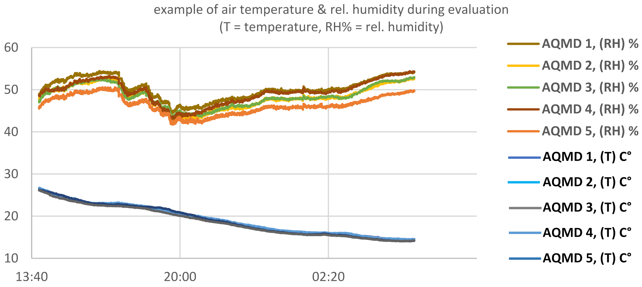
For the evaluation of the collected data, the measuring devices were compared to a recorded series of measurements from the reference measuring point “Taborstrasse”, managed by the “Municipal Department 22—Environmental Protection in Vienna (MA 22)”, shown in Figure 5. Reference data series were only available for particulate matter, temperature and humidity. To check the accuracy, the measuring devices were positioned next to each other at the reference point for 7 days, data were recorded, and the correlation was calculated by linear regression. The corresponding values are shown in Table 6 and Figure 6 shows the course of temperature and humidity during calibration as an example. Data that were recorded in the school were corrected according to the calculations and used for evaluations afterward. For the particulate matter sensors, a fixed intercept-value of 0 was chosen for calculation to increase the linear fit. As a demonstration, the correlation of the particulate matter sensors (OPCs) and the reference measuring point “Taborstrasse” are shown in Figure 7.
However, since the investigations on the effects of the green walls were carried out indoors, absolute concentration values of particulate matter concentration should not be used for conclusions, and only relative comparison between the different green walls is meaningful.
2.3. Evaluation Matrix
In order to gain an overview of the results obtained from the individual studies on the different plant species, a simple, custom evaluation matrix was created. Appropriate criteria and a grading system were selected. Since a comparison of the plant species with one another and with an option without plants was to be achieved, the average percentage difference to the reference without plants was evaluated for the hygrothermal comfort and the particulate matter/CO2 concentrations by ranking the values and then assigning points to each position. The ranking of the four variants assigns 4 points for 1st place, 3 points for 2nd place and so on. For the results of the reverberation time and the sound absorption coefficient, this evaluation was carried out for each examined frequency band, and then an overall evaluation was calculated.
The methods for the corresponding evaluations of the individual parameters and measurements performed are explained in the respective Results and Discussion Section (Section 3) for a more compact presentation.
3. Results and Discussion
Due to the different room-use scenarios of school classes and the fact that the examined room was partly unused due to COVID-19-related “home schooling”, the data were selected in such a way that the days on which the PM10 of all measuring devices reached a daily mean value (DMV) of at least 10 µg/m3 were considered. This way only days where usual utilization of the school and rooms was happening were analyzed. Table 7 shows the dimensions of the examined rooms and Table 8 shows the selected days accordingly.
3.1. Overview and Evaluation Matrix
Table 9 shows the evaluation matrix with the corresponding results of all considered parameters. The plant species golden pothos, followed by Boston fern, had the highest overall effect. The combination of plants and spider plant followed in third and fourth place. As observed in the table, compared to Boston fern, golden pothos offers a higher “performance”, especially with particulate matter, CO2 and acoustics.
3.2. Effects on Humidity and Air Temperature
From the measurements of air temperature and relative humidity carried out in one-minute-long intervals, 15 min average values were calculated. Before the actual evaluation, the recorded data were adjusted with the help of the calculated correlation factors, followed by data processing. The 15 min mean values were used directly to display the course; on the other hand, daily mean values (DMVs) were determined for statistical analysis. The evaluation of the measurement data of air temperature and relative air humidity in the preliminary project was based on the definition of hygrothermal comfort according to Frank [52]. Since the DIY green walls were located at a modest distance from each other in the room during the measurement data collection, no significant differences in the comfort diagram between the individual plants were to be expected. Therefore, the gain in absolute humidity was calculated according to Equation (1).
Equation (1). Calculation of absolute air humidity in g(H2O)/m3)
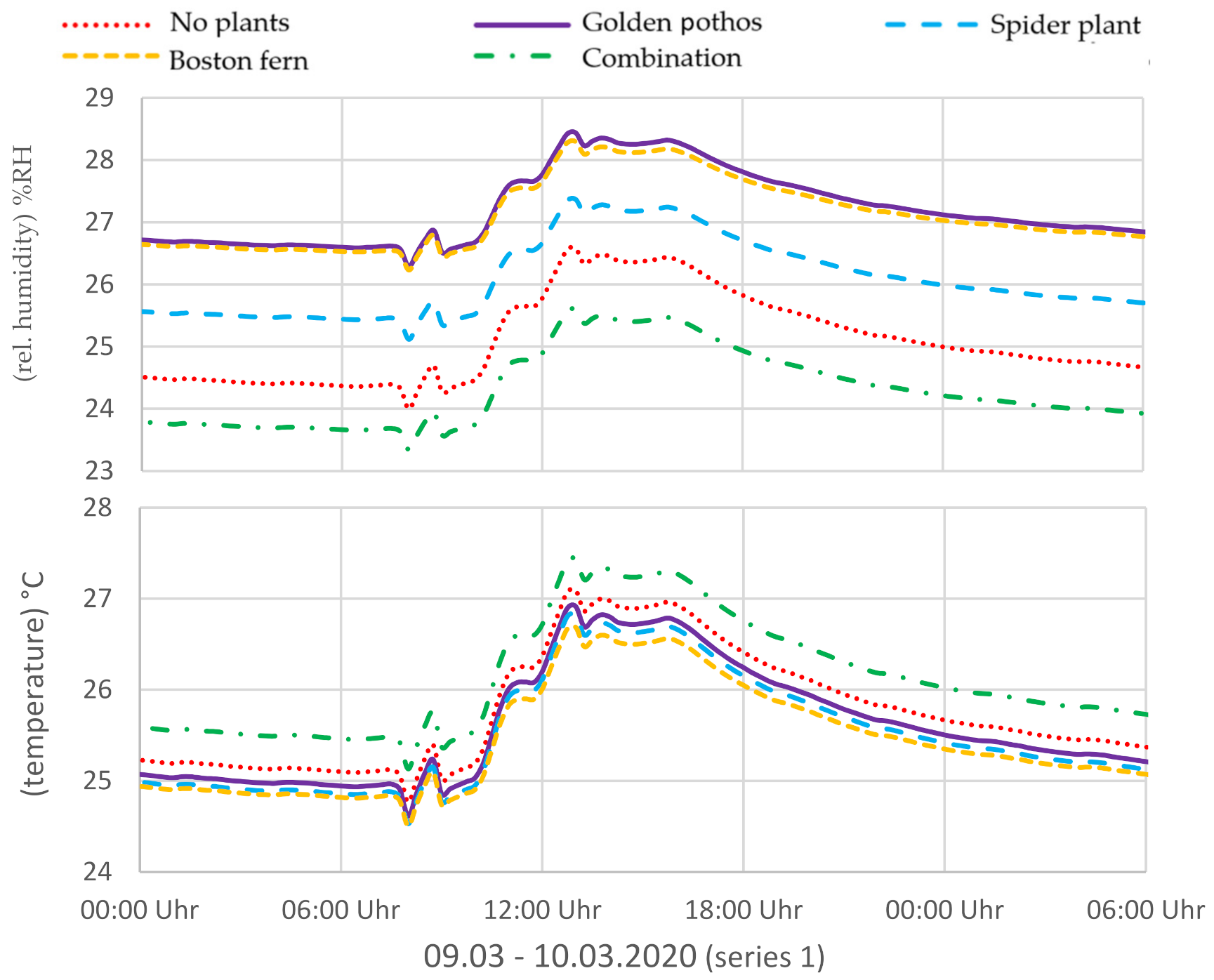
The data considering air temperature and relative air humidity are presented and evaluated in Figure 8. Observing this data set, it is noticeable that changes due to influences such as ventilation occur at the same time and the measured values constantly deviate from each other, which indicates that measurement uncertainty and variability are greater than the investigated green walls’ ability to cool their surroundings by transpiration.
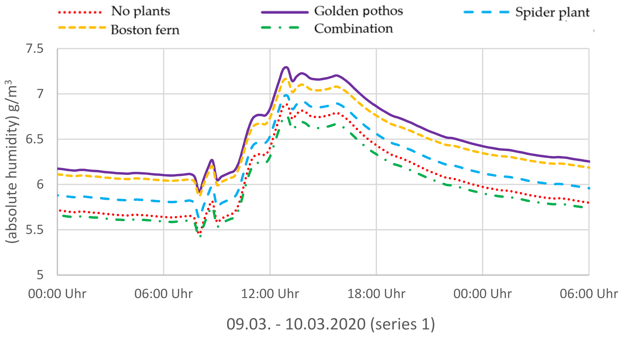
Since the relative humidity depends largely on the temperature, the absolute humidity was also calculated according to Equation (1). The values shown in Table 10 were calculated in order to describe the series of measurements statistically. Figure 9 shows the course of the absolute humidity on the selected example day.
Taking into account measurement uncertainty, the differences between the plants are not significant; however, golden pothos, followed by Boston fern and spider plant, reproducibly led to the greatest increases in (absolute) humidity in all measurement series, and the combination of plants does not seem to have any influence on humidity. The statistical analysis of the air temperature measurements, as shown in Table 11, is quite similar to the absolute humidity statistics. It is noticeable that Boston fern followed by golden pothos and spider plant consistently had a slight cooling effect, probably due to evapotranspiration; however, DIY green wall No. 4, the combination of plants, showed no influence. In conclusion, measurement uncertainty was greater than the measurable influence of the plants, and the suggested evapotranspiration could not be verified.
For further evaluation, the results of the humidity and temperature were considered independently of one another and the individual variants were ranked from large to small according to the value “% difference to no plants” and the points were assigned according to the ranking. Thus, considering absolute humidity, plant species got assigned the following points: golden pothos 4, Boston fern 3, spider plant 2 and combination of plants 1; considering temperature, the following points were assigned: Boston fern 4, spider plant 3, golden pothos 2 and combination of plants 1 point.
3.3. Effects on the Particulate Matter Concentration
The particulate matter concentration was measured with an “OPC”, optical particle counter. The theoretical basics of these measurements and the evaluations carried out can be found in detail in [53]. However, since only series of measurements for the PM10 and PM2.5 fraction were recorded for the calibration of the sensors, the evaluation was limited to these fractions. Before the actual evaluation, the recorded data were adjusted with the help of the calculated correlation factors, and the comparison of the plant species was carried out depending on the respective measurement series.
For the representation of the concentration as a function of time, 1 h mean values (HMVs) were calculated from the data recorded at intervals of one minute. To calculate the relative differences between the examined plant species, daily mean values (DMVs) were compared with one another.
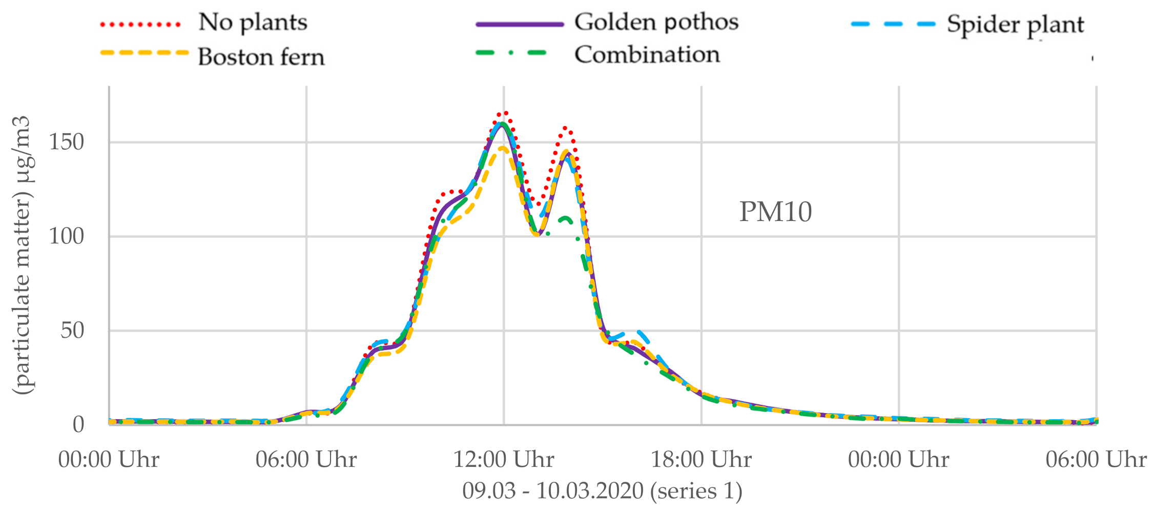
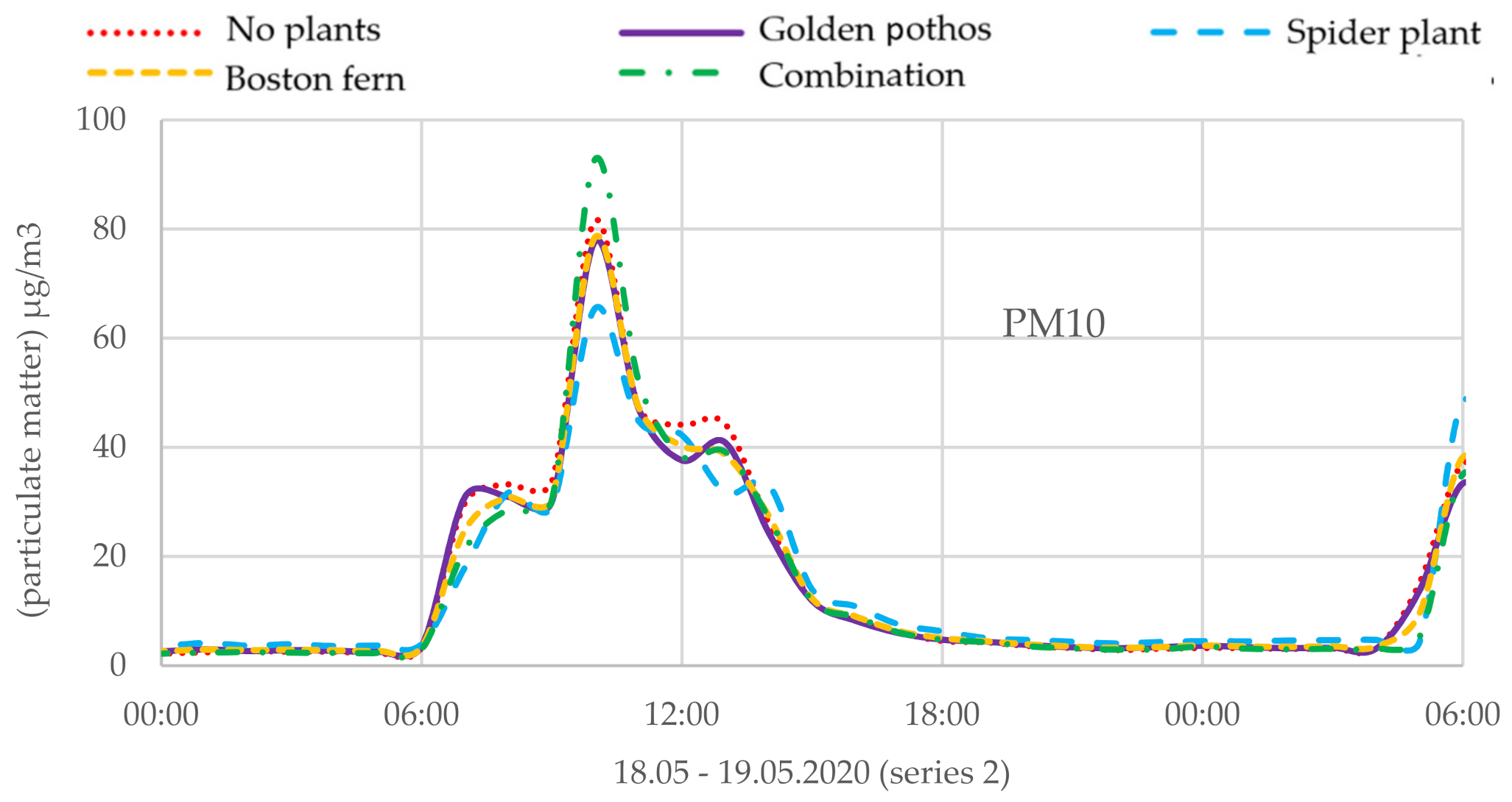
The evaluation and presentation of the particulate matter concentration were also based on the time periods listed in Table 6. While observing the course of the 1 h mean values of the particulate matter concentration PM10 fraction on an exemplary day, it can be seen that a concentration of approx. 40 µg/m3 was already present after two hours of use of the room and increased up to 160 µg/m3, as shown in Figure 10.
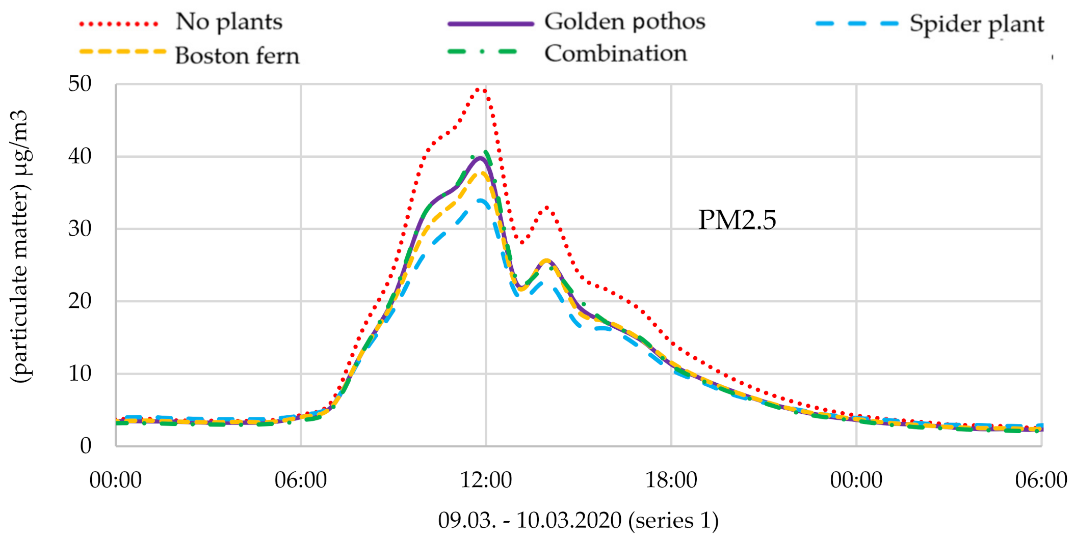
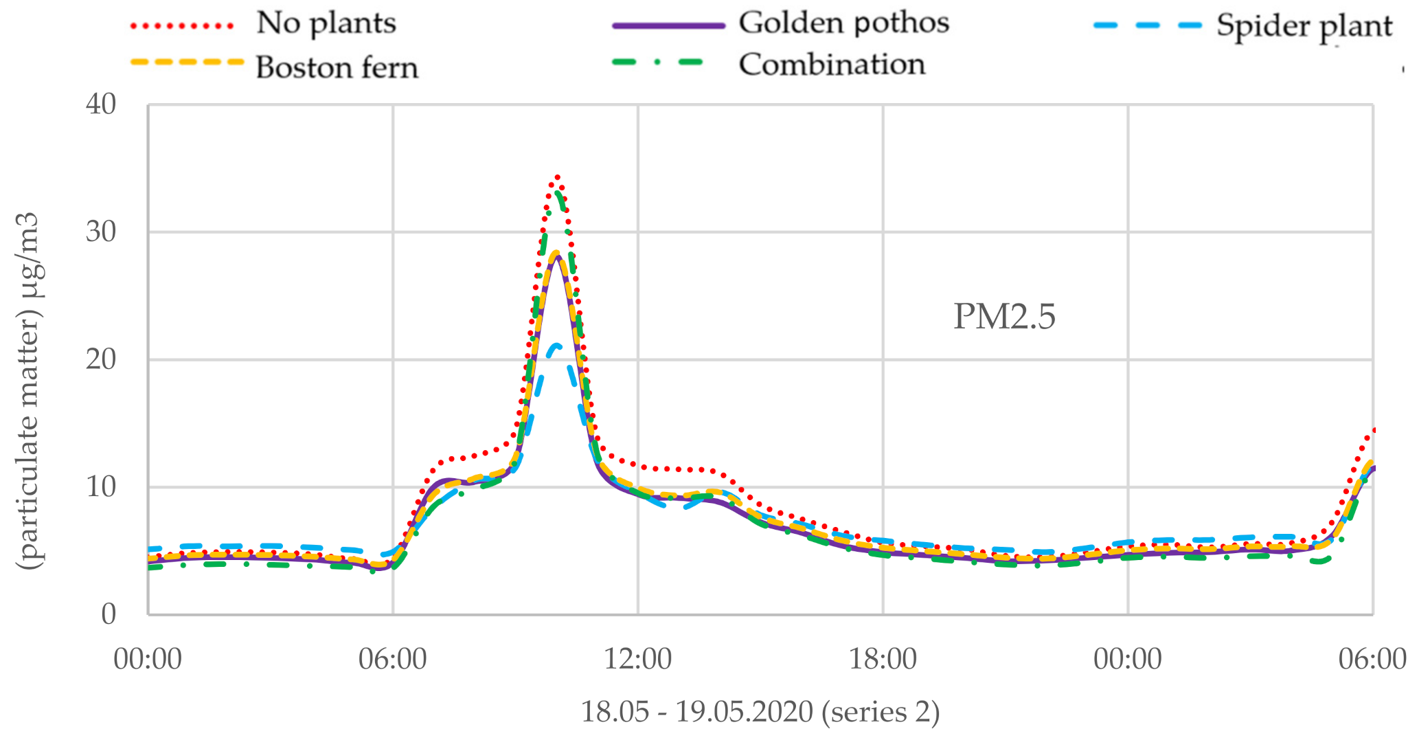
A similar trend can be seen when observing the PM2.5 fraction, with the absolute concentrations being lower and the effect of the greening being even more clearly recognizable. On the day shown in Figure 11, spider plant, in particular, seems to have a high effect, which is also visible in the statistical analysis shown in Table 12. Essentially, a lower concentration of particulate matter than the reference without plants was measured for all plant species with a similar prevalence. Measurement series 1 and 2 show a very similar picture: particles from fraction PM2.5 are reduced by up to 24% (spider plant) compared to the DMV, particles from fraction PM10 could be reduced by up to approx. 8%, and the effect seen in series 1 is significantly stronger.
Figure 12 and Figure 13 show another exemplary day on which the course of both particulate matter fractions looks very similar. This confirms a strong correlation between room use and particulate matter concentration. Thus, the comparatively low average concentrations in series 2 and 3 for both particulate matter fractions, as shown in Table 12, can also be explained. During this period (May and June), the classrooms presumably were regularly ventilated, which resulted in overall lower daily concentrations. The air humidity has a significant influence on the agglomeration and deposition of particles, whereby, for example, small, hygroscopic particles can grow into larger ones through absorption of water, and thus not only the effect of the greening but also weather might have had a significant influence. In the overall assessment, it is noticeable that all variants offer a comparable effect, but the combination of plants had the most balanced effect on both particulate matter fractions.
For the evaluation matrix, the results of both fractions were considered independently of one another and the individual variants were ranked from large to small according to the value “% difference to mean value no plants”, and then points were assigned according to the placement. Thus, with PM2.5, plants received the following points: Boston fern 4, golden pothos 3, spider plant 2 and combination of plants 1; with PM10, the following points were assigned: golden pothos 4, Boston fern 3, spider plant 2 and combination of plants 1 point.
3.4. Effects on CO2 Concentration
The measurement of the CO2 levels in the immediate vicinity of the plants was carried out with the aid of infrared sensors from the brand “ELT”. To represent the course, 15 min mean values of data recorded each minute were calculated. In order to calculate the relative differences between the examined plant species, daily mean values were compared with one another.
As was already established in [53], it is not possible to reliably quantify the influence of greenery on the basis of long-term measurements that were carried out in real school life. However, since the recording of the real conditions in a school class offers valuable information and conclusions about the microclimatic and measurement-related conditions and challenges, such measurements were carried out again.
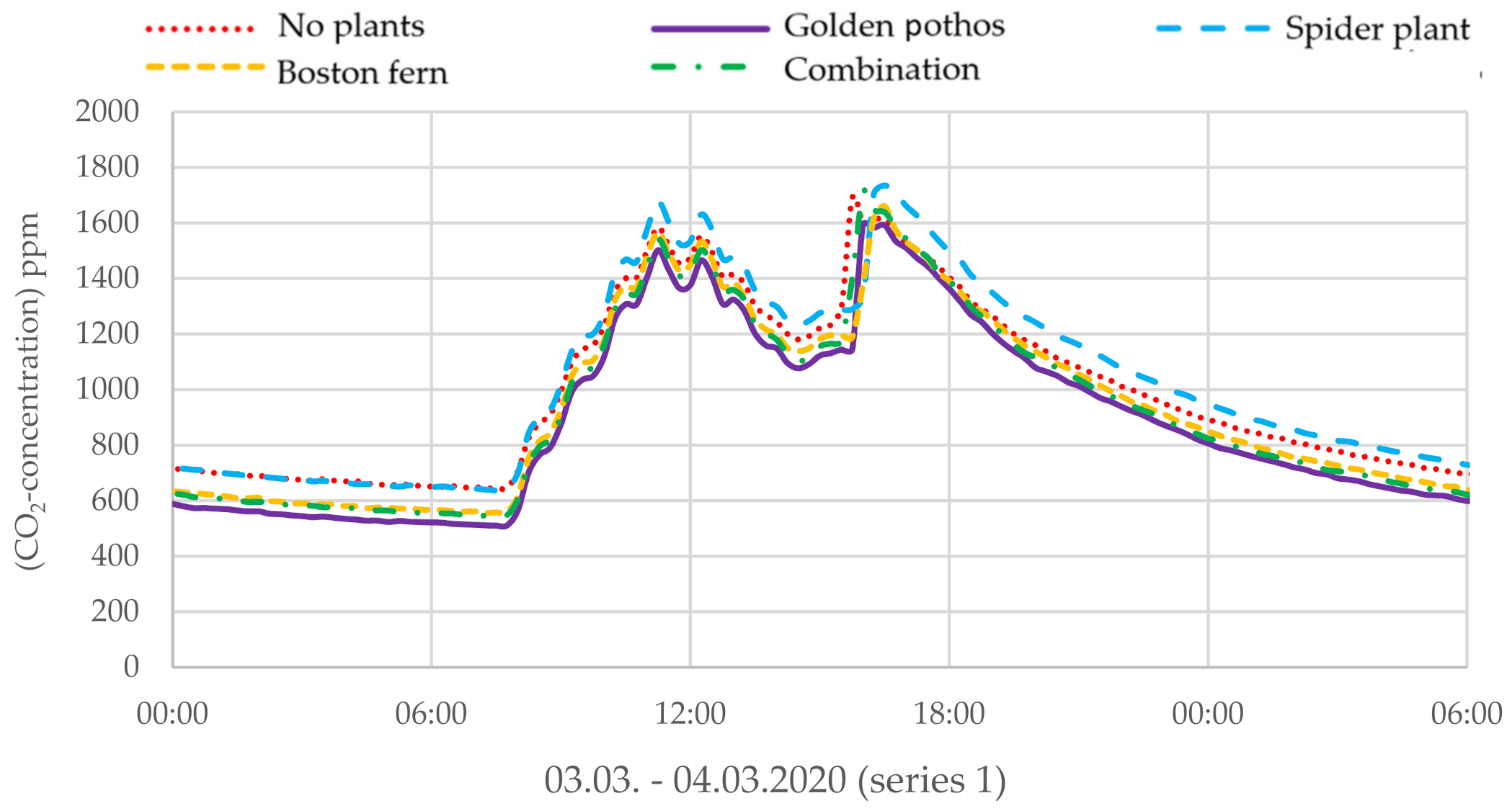
For the evaluation and presentation of the CO2 data, the days listed in Table 8 were initially used. Almost over the entire measuring range, the measured CO2 concentration on the DIY green walls was below the reference variant (no plants). In Figure 14, it can be seen that the CO2 concentration for golden pothos, Boston fern and the combination of plants is up to 200 ppm lower than the variant without plants.
In order to get a better picture of the long-term measured values, these were subjected to statistical evaluation, as can be seen in Table 13.
It was observed that series 1 shows a significantly lower reduction in CO2 concentration than series 2 and 3. This is probably due to the advanced growth of the plants, as well as probably dependent on the weather conditions, temperature and the incidence of light. This can be clearly seen in the case of Boston fern: In measurement series 1, the CO2 concentration was reduced by an average of 1%, but in measurement series 2, a reduction of 13% was measured. Overall, spider plant caused the smallest reduction in CO2 concentration. In measurement series 1, the concentration was increased by spider plant both during the day and the night.
Table 14 gives an overview of studies that examined the CO2 reduction of individual plant species under laboratory conditions. Suhaimi et. al. [50] found that, for example, the plant species Chlrophytum comosum, i.e., spider plant, increased the CO2 concentration in the test chamber by 0.1% even with an illumination of 700 Lux.
According to the evaluation matrix, the plants were assigned the following points: golden pothos 4, combination of plants 3, Boston fern 2 and spider plant 1 point. Since the combination of plants and Boston fern caused the same reduction on average during the day, they were also rated according to their performance at night: Boston fern −9% CO2, combination −12% CO2.
3.5. Effects on Room Acoustics
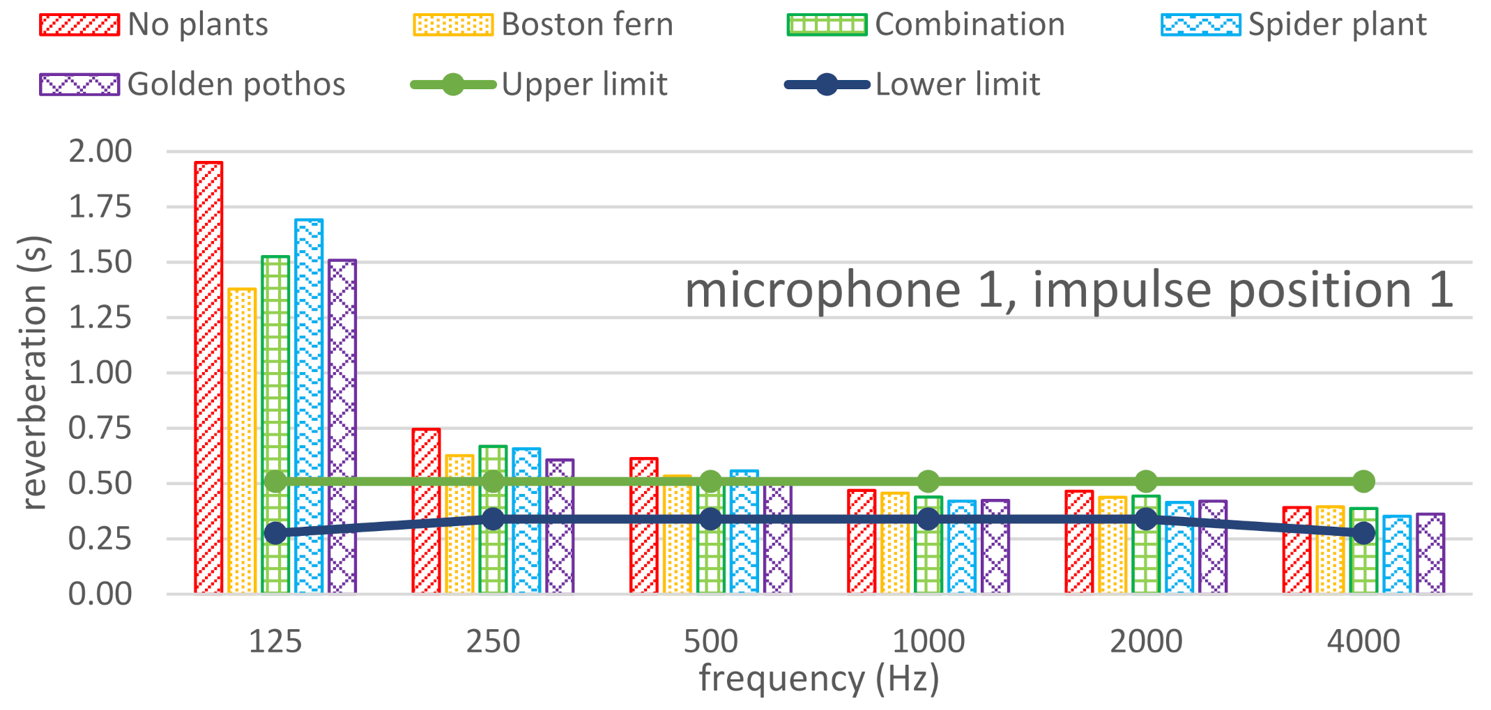
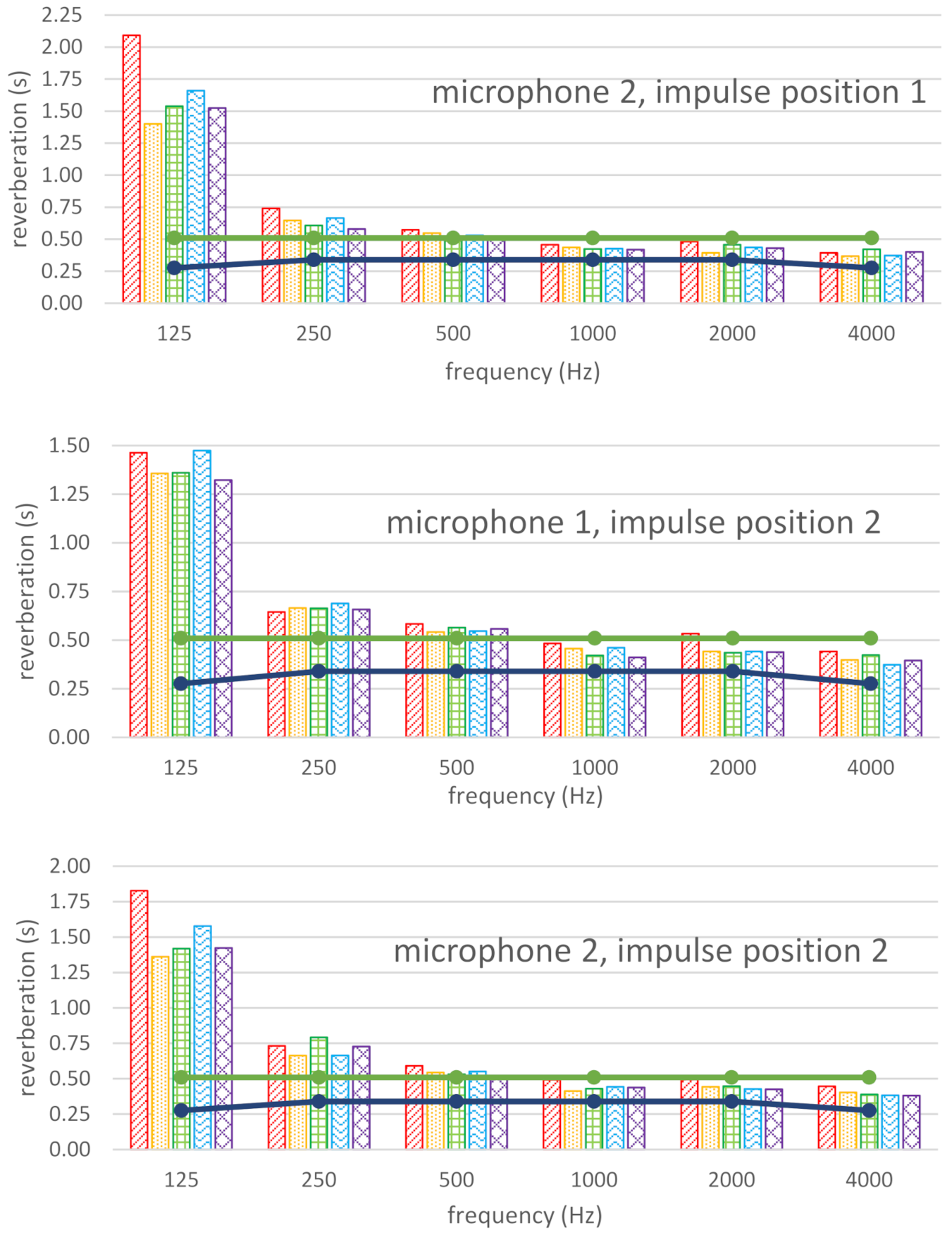
To determine the effects on the room acoustics, the reverberation time was measured based on ISO 3382-3 [55] in room 101. This room was chosen to increase the ratio of room volume to green-wall surface area and make the results more significant. Figure 15 shows the examined room with the DIY green wall and measuring equipment. In further studies, it should be investigated if the results are also applicable to larger rooms when scaling the green walls up accordingly. In [53], the theoretical fundamentals of acoustics and measurement of the reverberation time, as well as the calculation of the degree of sound absorption, are shown. For the measurements, the DIY green walls were brought into the room individually, and the reverberation time was determined using combinations of two microphone and two pulse positions for each of the species, as shown in Figure 16.
Specifically, two “Norsonic Nor140” sound analyzers were used as “microphones” for the measurements, distributed as asymmetrically as possible in the room according to the conditions, and the burst of a balloon filled with air was used as an “impulse”. To ensure uniformity between measurements, a hand pump and a specific volume of air were used.
The results are presented as a function of the frequency, and the relative deviation of the individual plant species from one another was calculated. In addition, the degree of sound absorption of the different plants was calculated and compared.
3.5.1. Reverberation Time
For the direct comparison of the measured values, as shown in Figure 17, the octave bands of the center frequencies 125 Hz, 250 Hz, 500 Hz, 1000 Hz, 2000 Hz and 4000 Hz were used in accordance with ÖNORM 8115-3 [56]. It can be seen that the reverberation time in the examined room is slightly shorter when equipped with green walls than without greening, which essentially confirms the results from [53]. Furthermore, the upper and lower limits according to ÖNORM 8115-3 [56] are shown.
Table 15 and Table 16 show the relative differences between the green walls with different plant species and the measurements without green walls. A positive value means a reduction in the reverberation time; a negative value indicates that no improvement in the room acoustics could be achieved. The greatest reduction can be seen in the case of golden pothos and Boston fern, whereby spider plant and combination of plants also cause a reduction in reverberation time. Only with impulse position 2 and sound analyzer (microphone) 1, deterioration of the reverberation time was observed in all plant variants at 250 Hz, which was the lowest with golden pothos followed by Boston fern, combination of plants and spider plant.
3.5.2. Sound Absorption Coefficient
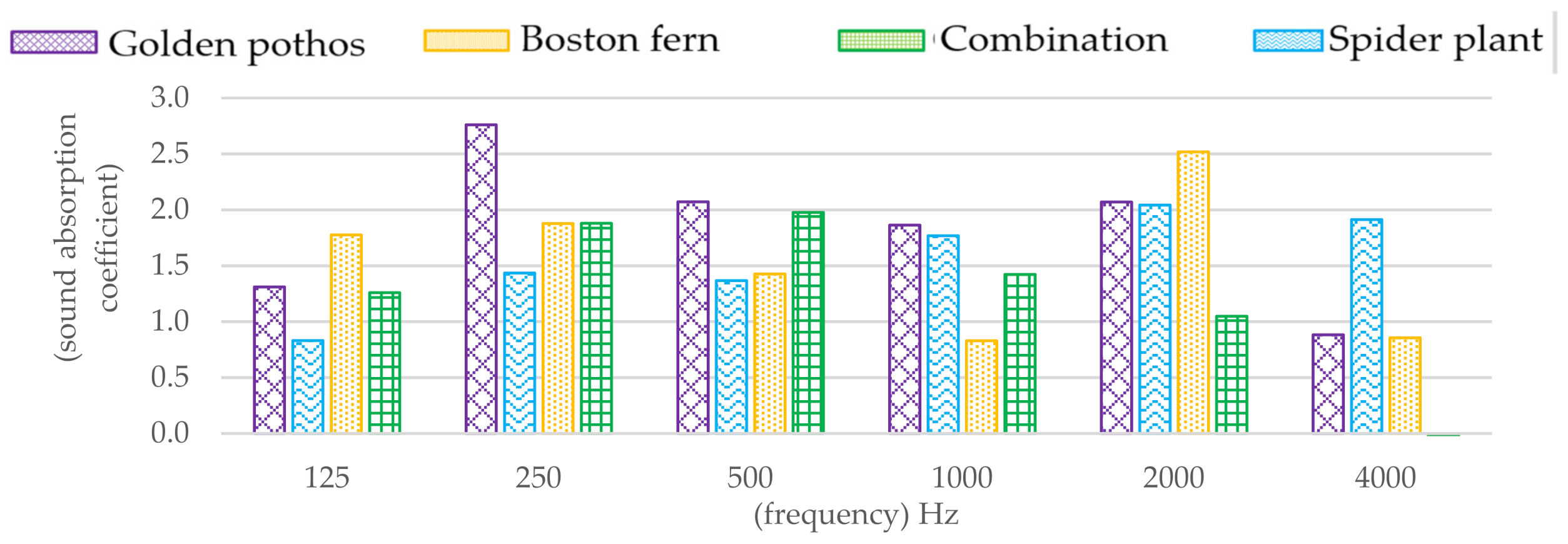
The sound absorption coefficient was calculated according to [53], for each plant species and the examined room without a green wall. In order to get a better overview of the data, the mean value for each of the plant species and for each pulse position was calculated from the values measured by devices and then compared. An analysis of the maximum values was then used to determine which plant had the greatest degree of absorption at the corresponding frequency band.
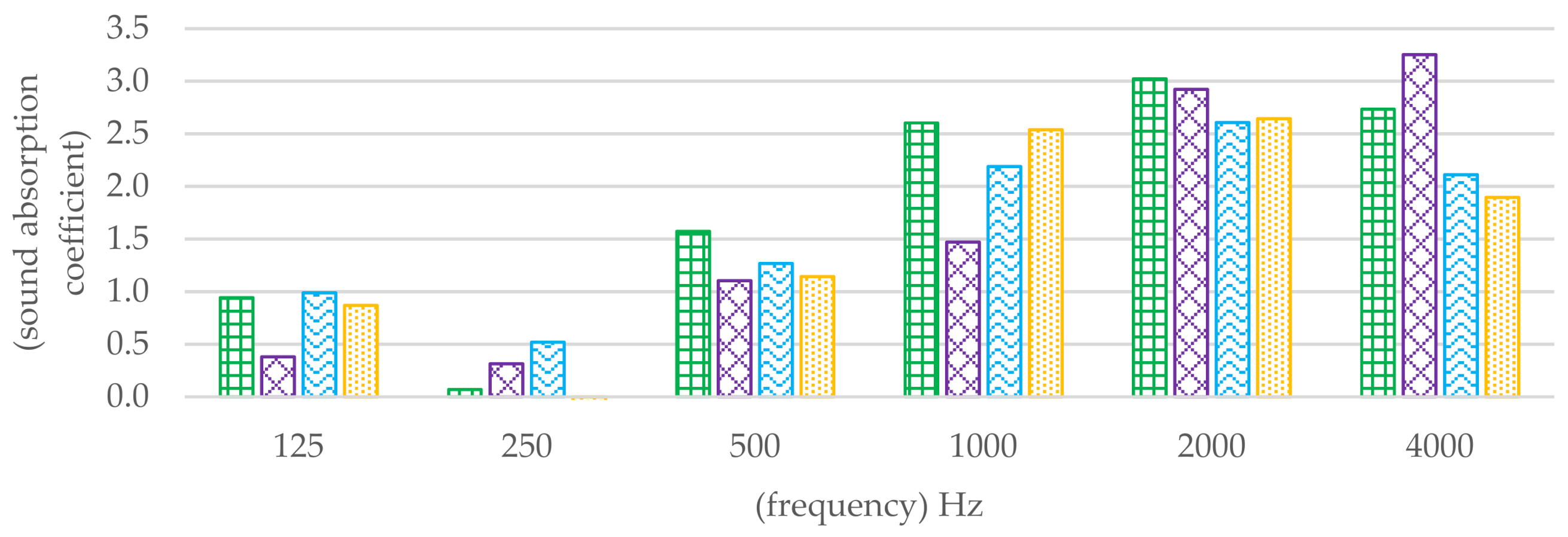
As already described in [53], values for the degree of sound absorption that are greater than 1 mean that theoretically more than 100% of the incoming sound energy was absorbed. In practice, this occurs when sound reaches a strongly absorbing sample and is therefore hardly reflected. The discontinuity in the wave field at the edge of the sample creates a diffraction effect that changes the sound field. This makes the sample a quarter of a wavelength larger for sound. The area increases and absorbs more sound energy per wall area than would have reached the wall. As can be seen in Table 17, golden pothos and Boston fern have the greatest effect in all frequency bands except at 4000 Hz, with clear differences between the pulse positions, which can be attributed to the fact that more direct sound is reflected in position 2 due to the proximity to the wall. Spider plant has the greatest sound absorption at 4000 Hz in both pulse positions.
At pulse position 1, depicted in Figure 18, no clear pattern was recognized for the sound absorption coefficient over all frequency bands due to the distribution of values.
At pulse position 2, shown in Figure 19, the sound absorption coefficient is particularly high in the audible range (around 1000 Hz). The lowest absorption takes place in the lower frequency ranges. Low-frequency bands only interact with heavier components, while higher frequencies also interact with lighter ones (such as plants or leaves) [53]. As a result, plant species with a large surface area and/or a growth habit that results in the construction being heavily covered should have a greater degree of sound absorption.
3.6. Effects on Mold Spore Concentration
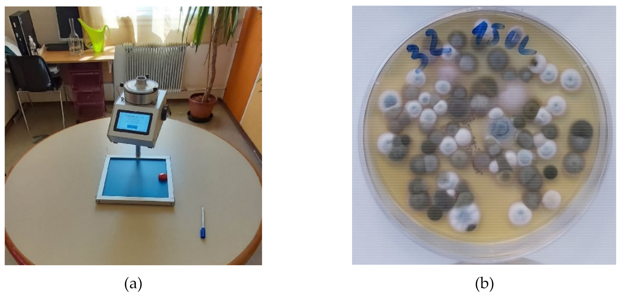
The mold spore concentration, determined and calculated as “Colony-forming units (CFU) per m3 of air”, was measured similarly to the reverberation time in room 101, which, with its area and room height, represents a room volume suitable for the investigations. For this purpose, the DIY green walls were introduced into the room one after the other, left in the unventilated room for 24 h, and then the room air was sampled with the help of an air sampler, shown in Figure 20, based on DIN ISO 16000-18 [57].
The loaded growing media was incubated at approx. 23 °C and 40% relative humidity, and the number of colony-forming units was counted after 3, 5 and 10 days. Malt extract agar and DG18 agar were used as growing media to determine the total spore count.
The correct execution of sampling the air essentially depends on the selected sample volume. The first series of measurements, with a sample volume of 300 or 150 L, partially led to an overload of the growing media (number of CFUs greater than 100 [58]). A second measurement campaign was carried out in January 2021 under the same conditions but with adapted sample volumes of 50 or 100 L. Since the investigations, carried out in this project, focused on the quantitative impact of the plants, the colony-forming units (CFUs) per m3 of room air were calculated for the individual measurements and then for assessment, compared with a value from the guidelines for prevention, recording and remediation of mold infestation in buildings of the Indoor Air Hygiene Commission of the German Federal Environment Agency [59].
These benchmarks were calculated from a variety of empirical data and are reported as the 95th percentile. This means that 95% of the measurement results were less than or equal to the specified value. Table 18 shows the corresponding values from the guidelines for the prevention, detection and remediation of mold infestation in buildings [59].
For measurement 1, the benchmark for the interior in winter and for measurement 2 in summer was used. The results are shown together with their standard deviation (e.g., ±46) and the number of measurements (e.g., n = 1) in Table 19 and Table 20.
The appropriate guideline value was not exceeded for any plant species and, in comparison to the reference measurement, it can generally be stated that the DIY green walls, regardless of the type of plant used, did not represent a source of mold spores.
4. Conclusions and Outlook
As the measurements and analysis showed, the DIY green walls built and set with the students represent an alternative in comparison to commercial greening systems. Due to simplicity and modular character of the construction, as well as the good availability of the necessary materials, such systems are easily adapted by schools and built as a part of or during the lessons.
The effect of such systems on specific pollutant concentrations and microclimate in the immediate vicinity of the plants was determined using metrological investigations. Because of these measurements and evaluations, it was shown that golden pothos, followed by Boston fern, had the highest positive influence on the examined parameters. However, due to high measurement variability and several uncertainties such as airflow, temperature gradient and limitation to the measurement of local effects, no clear result was reached, and the method of investigation needs to be improved when measuring under real-life circumstances.
Considered in more detail and if uncertainties are neglected, golden pothos had the greatest effect and delivered improvements in all measured parameters. Boston fern, in comparison, had worse performance in terms of particulate matter and CO2. The wall, planted with the combination of plants, on the other hand, only performed well in terms of particulate matter and CO2. Lastly, spider plant showed better effects in terms of temperature and humidity than the combination of plants. However, this plant performed overall worse, mainly due to the lack of effect on the reverberation time, CO2 and particulate matter concentration (PM2.5). In total, no clear winner was found due to the lack of reliable data.
Further, the green walls of golden pothos, Boston fern and combination of plants proved to be particularly robust and suitable for everyday school life. Spider plant, on the other hand, was more sensitive and therefore showed a greater need for care and was replaced with peace lily after the experiment.
The DIY green walls (regardless of the type of plant used) had no negative impact on the concentration of mold spores in the chosen test room, and none of the plant species had a significant impact on the total number of spores in the air. The measured concentrations also fell below the selected guide values of the Federal Environment Agency Germany, which confirms that the DIY green walls did not lead to any significant exposure or accumulation of mold spores.
Vertical indoor green structures thus make a valuable contribution to improving physical parameters associated with IAQ and human health. This type of green infrastructure therefore could be an important adaptation measure in schools to create healthy indoor learning spaces with high comfort and air quality. However, to measure the actual health impact of these structures on health in situ, a larger amount of measuring devices that are calibrated to the indoor environment is needed. To represent real-exposure scenarios, no investigation of IAQ or related parameters should be carried out without analyzing airflow around the examined green walls when measuring in the direct proximity of the plants. Furthermore, it should be noted that reference measurements have to be carried out in a (separate) room with no plants present to negate any cross-influences between plants and the reference. Supplementary data regarding the amount of light, watering and ventilation should also be recorded to quantify cost and energy efficiency and make green walls comparable to conventional air cleaning devices such as filters. Additionally, test setups should be adapted from earlier studies to make estimations of pollutant removal viable and comparison between studies possible.
Besides improving measurement methodology, as a next step regarding IAQ in general, investigating green infrastructure in combination with ventilation technology and integration of plants as a building service could be viable, since a combination and synergy will potentially lead to increased efficiency and effectiveness. With that, an analysis and comparison of the price/impact ratio are also needed. Furthermore, other air-quality-defining parameters, such as the TVOC, should be investigated to determine potential applications in environments with high VOC exposure, such as new buildings and workspaces. At the same time, research should focus on relatively cheap and affordable greening systems to increase accessibility of green infrastructure in general. In addition, the optimization of the combination of plants used in greening systems should also be examined further in real-life situations to give planners the possibility to choose plant species more easily. To achieve seamless integration in existing buildings, a guideline for the application of such systems could also be developed in a further step. To make sure that not only the effects on IAQ and hygrothermal comfort are considered but also the influence on, for example, acoustics is optimized, the design process of green infrastructure and further research regarding it should be carried out in multidisciplinary teams.
Author Contributions
Conceptualization, A.K. and J.H.; methodology, A.K., J.H. and A.P.; software, A.P.; validation, A.P., J.H.; formal analysis, A.P. and J.H.; investigation, A.P.; resources, A.P., J.H., E.S.; data curation, A.P. and E.S.; writing—original draft preparation, A.P., J.H., E.S.; writing—review and editing, A.P., J.H. and E.S.; visualization, A.P.; supervision, A.K. and J.H..; project administration, A.P.; funding acquisition, A.K and J.H. All authors have read and agreed to the published version of the manuscript.
Funding
This research was supported by the project “Weiterführende Untersuchungen und Monitoring der grünen Wände am GRG7 Kandlgasse/Further investigations and monitoring of the green walls at GRG7 Kandlgasse”, KFI:607419-0002-III-I3-2019, funded by the Austrian Federal Ministry for Climate Action, Environment, Energy, Mobility, Innovation and Technology (BMK).
Institutional Review Board Statement
Not applicable.
Informed Consent Statement
Not applicable.
Data Availability Statement
The data presented in this study are available on request from the corresponding author. The data are not publicly available due to privacy and legal constraints.
Acknowledgments
The authors acknowledge TU Wien Bibliothek for financial support through its Open Access Funding Programme.
Conflicts of Interest
The authors declare no conflict of interest.
References
- American Lung Association. When You Can’t Breathe, Nothing Else Matters. Air Quality. 2001. Available online: www.lungusa.org/air/ (accessed on 1 July 2021).
- Lu, C.; Deng, Q.; Li, Y.; Sundell, J.; Norbäck, D. Outdoor air pollution, meteorological conditions and indoor factors in dwellings in relation to sick building syndrome (SBS) among adults in China. Sci. Total Environ. 2016, 560–561, 186–196. [Google Scholar] [CrossRef] [Green Version]
- Holgate, S.T. ‘Every breath we take: The lifelong impact of air pollution’—A call for action. Clin. Med. J. R. Coll. Physicians Lond. 2017, 17, 8–12. [Google Scholar] [CrossRef] [PubMed] [Green Version]
- Marć, M.; Śmiełowska, M.; Namiesnik, J.; Zabiegała, B. Indoor air quality of everyday use spaces dedicated to specific purposes—A review. Environ. Sci. Pollut. Res. 2018, 25, 2065–2082. [Google Scholar] [CrossRef] [Green Version]
- Bandehali, S.; Miri, T.; Onyeaka, H.; Kumar, P. Current state of indoor air phytoremediation using potted plants and green walls. Atmosphere 2021, 12, 473. [Google Scholar] [CrossRef]
- Ryu, J.; Kim, J.J.; Byeon, H.; Go, T.; Lee, S.J. Removal of fine particulate matter (PM2.5) via atmospheric humidity caused by evapotranspiration. Environ. Pollut. 2019, 245, 253–259. [Google Scholar] [CrossRef] [PubMed]
- European Comission. Indoor Air Pollution: New EU Research Reveals Higher Risks Than Previously Thought; European Comission: Brussels, Belgium, 2003; Available online: https://ec.europa.eu/commission/presscorner/detail/en/IP_03_1278 (accessed on 10 July 2021).
- Derwent, R.; Hjellbrekke, A.-G. Air Quality in Europe—2019 Report 1994–2019 EEA Report; Brussels, Belgium, 2019; Available online: https://www.eea.europa.eu/publications/air-quality-in-europe-2019 (accessed on 10 July 2021).
- World Health Organization. Burden of Disease from the Joint Effects of Household and Ambient Air Pollution for 2016 Summary of Results; World Health Organization: Geneva, Switzerland, 2018; Volume 2, Available online: https://www.who.int/airpollution/data/AP_joint_effect_BoD_results_May2018.pdf (accessed on 10 July 2021).
- Guieysse, B.; Hort, C.; Platel, V.; Muñoz, R.; Ondarts, M.; Revah, S. Biological treatment of indoor air for VOC removal: Potential and challenges. Biotechnol. Adv. 2008, 26, 398–410. [Google Scholar] [CrossRef] [PubMed]
- Burge, P.S. Sick building syndrome. Occup. Environ. Med. 2004, 61, 185–190. [Google Scholar] [CrossRef] [PubMed] [Green Version]
- Cincinelli, A.; Martellini, T.; Amore, A.; Dei, L.; Marrazza, G.; Carretti, E.; Belosi, F.; Ravegnani, F.; Leva, P. Measurement of volatile organic compounds (VOCs) in libraries and archives in Florence (Italy). Sci. Total Environ. 2016, 572, 333–339. [Google Scholar] [CrossRef]
- Luengas, A.; Barona, A.; Hort, C.; Gallastegui, G.; Platel, V.; Elias, A. A review of indoor air treatment technologies. Rev. Environ. Sci. Bio/Technol. 2015, 14, 499–522. [Google Scholar] [CrossRef]
- Hubbard, H.F.; Coleman, B.K.; Sarwar, G.; Corsi, R.L. Effects of an ozone-generating air purifier on indoor secondary particles in three residential dwellings. Indoor Air 2005, 15, 432–444. [Google Scholar] [CrossRef]
- U. und W. Arbeitskreis Innenraumluft im Bundesministerium für Land-und Forstwirtschaft, Richtlinie zur Bewertung der Innenraumluft. Vienna, Austria, 2011. Available online: https://www.bmk.gv.at/themen/klima_umwelt/luft/innenraum/rl_luftqualitaet.html (accessed on 10 July 2021).
- Gossauer, E.; Wagner, A. Nutzerzufriedenheit und Komfort am Arbeitsplatz—Ergebnisse einer Feldstudie in Bürogebäuden. Bauphysik 2008, 30, 445–452. [Google Scholar] [CrossRef]
- Carrer, P.; Wolkoff, P. Assessment of Indoor Air Quality Problems in Office-Like Environments: Role of Occupational Health Services. Int. J. Environ. Res. Public Health 2018, 15, 741. [Google Scholar] [CrossRef] [Green Version]
- Hemmes, J.H.; Winkler, K.C.; Kool, S.M. Virus survival as a seasonal factor in influenza and poliomyelitis. Antonie Van Leeuwenhoek 1962, 28, 221–233. [Google Scholar] [CrossRef] [PubMed]
- Von Hahn, N. Trockene Luft und ihre Auswirkungen auf die Gesundheit—Ergebnisse einer Literaturstudie. In Gefahrstoffe Reinhaltung der Luft; Baudirektion Kanton Zürich: Zurich, Germany, 2007; Volume 67. [Google Scholar]
- Mäkinen, T.M.; Juvonen, R.; Jokelainen, J.; Harju, T.H.; Peitso, A.; Bloigu, A.; Silvennoinen-Kassinen, S.; Leinonen, M.; Hassi, J. Cold temperature and low humidity are associated with increased occurrence of respiratory tract infections. Respir. Med. 2009, 103, 456–462. [Google Scholar] [CrossRef] [PubMed] [Green Version]
- Noti, J.D.; Blachere, F.M.; McMillen, C.M.; Lindsley, W.; Kashon, M.L.; Slaughter, D.R.; Beezhold, D. High Humidity Leads to Loss of Infectious Influenza Virus from Simulated Coughs. PLoS ONE 2013, 8, e57485. [Google Scholar] [CrossRef]
- Gardinassi, L.G.; Simas, P.V.M.; Salomão, J.B.; Durigon, E.L.; Trevisan, D.M.Z.; Cordeiro, J.A.; Lacerda, M.N.; Rahal, P.; De Souza, F.P. Seasonality of viral respiratory infections in Southeast of Brazil: The influence of temperature and air humidity. Braz. J. Microbiol. 2012, 43, 98–108. [Google Scholar] [CrossRef]
- Lowen, A.C.; Steel, J. Roles of Humidity and Temperature in Shaping Influenza Seasonality. J. Virol. 2014, 88, 7692–7695. [Google Scholar] [CrossRef] [Green Version]
- Arundel, A.V.; Sterling, E.M.; Biggin, J.H.; Sterling, T.D. Indirect health effects of relative humidity in indoor environments. Environ. Health Perspect. 1986, 65, 351–361. [Google Scholar] [CrossRef] [Green Version]
- United States Environmental Protection Agency. Introduction to Indoor Air Quality. 2013. Available online: https://www.epa.gov/indoor-air-quality-iaq/introduction-indoor-air-quality (accessed on 10 July 2021).
- Han, K.-T. An Overview of the Positive Influences of Natural Landscapes on Humans; Lambert Academic Publishing: Saarbrücken, Germany, 2011. [Google Scholar]
- Dravigne, A.; Waliczek, T.M.; Lineberger, R.; Zajicek, J. The Effect of Live Plants and Window Views of Green Spaces on Employee Perceptions of Job Satisfaction. HortScience 2008, 43, 183–187. [Google Scholar] [CrossRef] [Green Version]
- Doxey, J.S.; Waliczek, T.M.; Zajicek, J.M. The Impact of Interior Plants in University Classrooms on Student Course Performance and on Student Perceptions of the Course and Instructor. HortScience 2009, 44, 384–391. [Google Scholar] [CrossRef]
- Han, K.-T. Influence of passive versus active interaction with indoor plants on the restoration, behaviour and knowledge of students at a junior high school in Taiwan. Indoor Built Environ. 2017, 27, 818–830. [Google Scholar] [CrossRef]
- Hollands, J.; Korjenic, A. Indirect Economic Effects of Vertical Indoor Green in the Context of Reduced Sick Leave in Offices. Sustainability 2021, 13, 2256. [Google Scholar] [CrossRef]
- Tudiwer, D.; Korjenic, A. The effect of an indoor living wall system on humidity, mould spores and CO2-concentration. Energy Build. 2017, 146, 73–86. [Google Scholar] [CrossRef]
- Wolverton, B. The Role of Plants and Microorganisms in Assuring a Future Supply of Clean Air and Water; Natl Aeronautics Space Admin, Natl Space Technol. Lab., Stennis Space Center: Boston, MA, USA, 1984. [Google Scholar]
- Godish, T.; Guindon, C. An assessment of botanical air purification as a formaldehyde mitigation measure under dynamic laboratory chamber conditions. Environ. Pollut. 1989, 62, 13–20. [Google Scholar] [CrossRef]
- Fjeld, T.; Bonnevie, C. The Effect of Plants and Artificial Day-Light on the Well-Being and Health of Office Workers; School Children and Health Care Personnel, Medicine, Lippincott: Philadelphia, PA, USA, 2002. [Google Scholar]
- Wolverton, B.C.; Johnson, A.; Bounds, K. Interior Landscape Plants for Indoor Air Pollution Abatement; National Aeronautics and Space Administration, NASA: Washington, DC, USA, 1989.
- Coward, M.; Ross, D.; Coward, S.; Cayless, S.; Raw, G. Pilot Study to Assess the Impact of Green Plants on NO2 Levels in Homes. In Building Research Establishment Note; N154/96; Building Research Establishment: Watford, UK, 1996. [Google Scholar]
- Orwell, R.L.; Wood, R.L.; Tarran, J.; Torpy, F.; Burchett, M.D. Removal of Benzene by the Indoor Plant/Substrate Microcosm and Implications for Air Quality. Water Air Soil Pollut. 2004, 157, 193–207. [Google Scholar] [CrossRef]
- Wood, R.A.; Burchett, M.D.; Alquezar, R.; Orwell, R.L.; Tarran, J.; Torpy, F. The Potted-Plant Microcosm Substantially Reduces Indoor Air VOC Pollution: I. Office Field-Study. Water Air Soil Pollut. 2006, 175, 163–180. [Google Scholar] [CrossRef]
- Yoo, M.H.; Kwon, Y.J.; Son, K.-C.; Kays, S.J. Efficacy of Indoor Plants for the Removal of Single and Mixed Volatile Organic Pollutants and Physiological Effects of the Volatiles on the Plants. J. Am. Soc. Hortic. Sci. 2006, 131, 452–458. [Google Scholar] [CrossRef] [Green Version]
- Kim, K.J.; Kil, M.J.; Song, J.S.; Yoo, E.H.; Son, K.-C.; Kays, S.J. Efficiency of Volatile Formaldehyde Removal by Indoor Plants: Contribution of Aerial Plant Parts versus the Root Zone. J. Am. Soc. Hortic. Sci. 2008, 133, 521–526. [Google Scholar] [CrossRef] [Green Version]
- Irga, P.; Torpy, F.; Burchett, M. Can hydroculture be used to enhance the performance of indoor plants for the removal of air pollutants? Atmos. Environ. 2013, 77, 267–271. [Google Scholar] [CrossRef]
- Knowles, L.; MacLean, P.; Rosato, M.; Stanley, C.; Volpe, S.; Yousif, D. Living Wall: A Feasibility Study for the Student Life Centre; Final Report; University of Waterloo: Waterloo, ON, Canada, 2002. [Google Scholar]
- Tarran, J.; Torpy, F.; Burchett, M. Use of living pot-plants to cleanse indoor air—Research review. In Proceedings of the IAQVEC 2007 6th International Conference on Indoor Air Quality, Ventilation and Energy Conservation in Buildings: Sustainable Built Environment, Sendai, Japan, 28–31 October 2007; Volume 3. [Google Scholar]
- Pennisi, S.V.; van Iersel, M. Quantification of Carbon Assimilation of Plants in Simulated and In Situ Interiorscapes. HortScience 2012, 47, 468–476. [Google Scholar] [CrossRef] [Green Version]
- Davis, M.; Tenpierik, M.; Ramírez, F.; Pérez, M. More than just a Green Facade: The sound absorption properties of a vertical garden with and without plants. Build. Environ. 2017, 116, 64–72. [Google Scholar] [CrossRef] [Green Version]
- Van Renterghem, T.; Botteldooren, D.; Verheyen, K. Road traffic noise shielding by vegetation belts of limited depth. J. Sound Vib. 2012, 331, 2404–2425. [Google Scholar] [CrossRef] [Green Version]
- Azkorra, Z.; Pérez, G.; Coma, J.; Cabeza, L.F.; Bures, S.; Alvaro, J.E.; Erkoreka, A.; Urrestarazu, M. Evaluation of green walls as a passive acoustic insulation system for buildings. Appl. Acoust. 2015, 89, 46–56. [Google Scholar] [CrossRef] [Green Version]
- Hutter, H.; Moshammer, H.; Wallner, P.; Hohenblum, P.; Uhl, M.; Scharf, S.; Gundacker, C.; Wittmann, K.; Tappler, P.; Piegler, B.; et al. Indoor air quality: Influence on health of schoolchildren in Austria. In Proceedings of the Joint Annual Conference of the International Society for Environmental Epidemiology (ISEE) and the International Society of Exposure Analysis (ISEA), Pasadena, CA, USA, 12–16 October 2008. [Google Scholar]
- Korjenc, A.; Tudiwer, D.; Hollands, J. Grüne Zukunft Schule; Endbericht; Klima und Energiefonds. 2020. Available online: https://smartcities.at/stadt-projekte/smart-cities/#/gruenezukunftschulen (accessed on 10 July 2021).
- Suhaimi, M.M.; Leman, A.; Afandi, A.; Hariri, A.; Idris, A.F.; Dzulkifli, S.M.; Gani, P. Effectiveness of Indoor Plant to Reduce CO2 in Indoor Environment. In Proceedings of the MATEC Web of Conferences, Sibiu, Romania, 7–9 June 2017; Volume 103, p. 5004. [Google Scholar]
- Cao, Y.; Li, F.; Wang, Y.; Yu, Y.; Wang, Z.; Liu, X.; Ding, K. Assisted deposition of PM2. 5 from indoor air by ornamental potted plants. Sustainability 2019, 11, 2546. [Google Scholar] [CrossRef] [Green Version]
- Frank, W. Raumklima und Thermische Behaglichkeit; Berichte aus der Bauforsch; Ernst & Sohn Verlag: Berlin, Germany, 1975; Volume 104. [Google Scholar]
- Korjenic, A. GrünPlusSchule@Ballungszentrum Hocheffiziente Fassaden-und Dachbegrünung mit Photovoltaik Kombination; optimale Lösung für die Energieeffizienz in gesamtökologischer Betrachtung. In Endbericht, Stadt der Zukunft, FFG/BMVIT; Wien, Austria, 2018; Available online: https://nachhaltigwirtschaften.at/de/sdz/projekte/gruenplusschule-ballungszentrum-hocheffiziente-fassaden-und-dachbegruenung-mit-photovoltaik-kombination-optimale-loesung-fuer-die-energieeffizienz-in-gesamtoekologischer-betrachtung.php (accessed on 10 July 2021).
- Sevik, H.; Cetin, M.; Guney, K.; Belkayali, N. The Influence of House Plants on Indoor CO2. Polish J. Environ. Studies 2017, 26, 1643–1651. [Google Scholar] [CrossRef]
- DIN EN ISO 3382-3:2012-05. In Acoustics—Measurement of Room Acoustic Parameters—Part 3: Open Plan Offices (ISO 3382-3:2012), German version EN ISO 3382-3:2012; Normenausschuss Akustik, DIN Deutsches Institut für Normen e.V.: Berlin, Germany, 2012.
- ÖNORM B 8115-3. In Schallschutz und Raumakustik im Hochbau—Teil 3: Raumakustik; Austrian Standards Institute: Vienna, Austria, 2005.
- Norm, D. Innenraumluftverunreinigungen—Teil 18: Nachweis und Zählung von Schimmelpilzen—Probenahme Durch Impaktion (16000-18:2008); DIN Deutsches Institut für Normen e.V.: Berlin, Germany, 2012. [Google Scholar]
- Norm, D. Innenraumluftverunreinigungen—Teil 17: Nachweis und Zählung von Schimmelpilzen—Kultivierungsverfahren (ISO 16000-17:2008); DIN Deutsches Institut für Normen e.V.: Berlin, Germany, 2010. [Google Scholar]
- Guidelines for Prevention, Recording and Remediation of Mold Infestation in Buildings; Indoor Air Hygiene Commission of the German Federal Environment Agency: Bonn, Germany, 2017.
Figure 1.
(a) 3D design of the DIY green wall and (b) exploded view of a trough (right).

Figure 2.
Different plant species from left to right: golden pothos, Boston fern, spider plant and combination of plants.
Figure 2.
Different plant species from left to right: golden pothos, Boston fern, spider plant and combination of plants.

Figure 3.
DIY green wall (spider plant) with installed AQMD.

Figure 4.
DIY green walls in Classroom 121 (from left to right Boston fern, golden pothos, peace lily, combination of plants).
Figure 4.
DIY green walls in Classroom 121 (from left to right Boston fern, golden pothos, peace lily, combination of plants).

Figure 5.
Reference measuring point Taborstrasse, Vienna.

Figure 6.
The course of temperature and humidity during evaluation procedure.

Figure 7.
Correlation of the used particulate matter sensors (OPCs) and the reference measuring point “Taborstrasse”.
Figure 7.
Correlation of the used particulate matter sensors (OPCs) and the reference measuring point “Taborstrasse”.

Figure 8.
Relative air humidity and air temperature in period from 9 March until 10 March 2020.

Figure 9.
Absolute air humidity in period from 9 March until 10 March 2020.

Figure 10.
Course of the particulate matter concentration fraction PM10 on 9 March 2020.

Figure 11.
Course of particulate matter concentration fraction PM2.5 on 9 March 2020.

Figure 12.
Course of the particulate matter concentration fraction PM10 on 18 May 2020.

Figure 13.
Course of the particulate matter concentration fraction PM2.5 on 18 May 2020.

Figure 14.
Course of the CO2 concentration in the period between 3 and 4 March 2020.

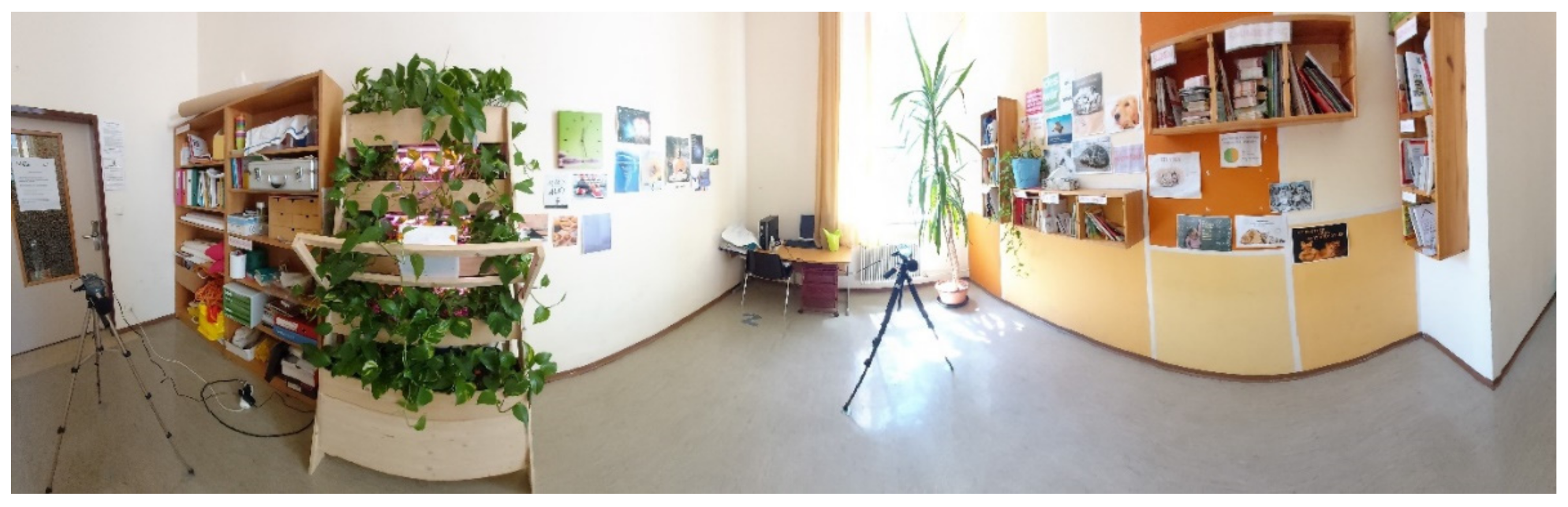
Figure 15.
A 360° picture of room 101 with the greening wall in place and two microphones to measure the reverberation time.
Figure 15.
A 360° picture of room 101 with the greening wall in place and two microphones to measure the reverberation time.

Figure 16.
(a) Floor plan room 101 and (b) photo of room 101 with installed microphones.

Figure 17.
Results of reverberation time measurements in comparison.


Figure 18.
Sound absorption coefficient, impulse position 1.

Figure 19.
Sound absorption coefficient, impulse position 2.

Figure 20.
(a) Air sampler in the sampled room; (b) incubated growing medium.


Table 1.
Selected plants for the DIY green walls.
| DIY Green Wall | Plant Species | Designation |
|---|---|---|
| 1 | Epipremnum aureum | Golden pothos |
| 2 | Nephrolepis exalta | Boston fern |
| 3 | Chlorophytum comosum | Spider plant |
| 4 | Nephrolepis exalta, Chlorophytum comosum, Ficus benjamina, Anthurium andreanum, Yucca filomentosa, Asplenium sp., Dieffenbachia sp., Spathiphyllum sp. | Combination |
| Plant Species | CO2 | ||
|---|---|---|---|
| Result | Reference | Comment | |
| Epipremnum aureum | ~7.5 ppm decrease in total CO2/h/plant | [50] | single potted plant, pot diameter = 17cm, @ 300 Lux, ~25 °C, ~8 h experiment in test chamber |
| Nephrolepis exalta | ~7.5 ppm decrease in total CO2/h/plant | ||
| Chlorophytum comosum | ~0,1 ppm increase in total CO2/h/plant | ||
| Combination | ~1 ppm decrease in total CO2/h/m2 | [31] | 5 m2 living wall, ~70% coverage with mixed plants |
Table 3.
Estimation of PM level reduction according to literature [51].
Table 3.
Estimation of PM level reduction according to literature [51].
| Plant Species | Particulate Matter | |||
|---|---|---|---|---|
| Result | Reference | Comment | ||
| Epipremnum aureum | ~40% PM2.5 removal rate | [51] | Single potted plant; ~20 °C, ~3 h experiment in 40 × 30 × 50 cm test chamber, concentration at start: ~200 μg/m3 | |
| Nephrolepis exalta | ~25% PM2.5 removal rate | Value adopted and estimated from plant with similar morphology | ||
| Chlorophytum comosum | ~30% PM2.5 removal rate | |||
| Combination | ~25% PM2.5 removal rate | Mean value of all examined species | ||
| No plants | ~20% PM2.5 removal rate | |||
Table 4.
Sensors used in AQMD.
| Measurement | Sensor Name | Accuracy |
|---|---|---|
| Particulate matter (PM10, PM2.5) | Alphasense OPC-N3 | no data available, see Table 6 |
| Carbon dioxide (CO2) | ELT D-300G-3V | ±30 ppm ± 3% of reading |
| Temperature | Sensirion STS30 | ±0.2 at 0–65 °C |
| Relative humidity | Sensirion SHT30 | ±2 at 10–90% RH |
Table 5.
Overview of the locations of the greening systems.
| Period of Time | Location | Comment |
|---|---|---|
| Week 50 (2019)–Week 8 (2020) | Corridor in front of the music room | |
| Week 9 (2020)–Week 25 (2020) | Classroom 121 | |
| Week 25 (2020)–Week 27 (2020) | Room 101 | Reverberation time and mold spores |
| Week 28 (2020)–Week 2 (2021) | Classroom 121 | |
| Week 2 (2021)–Week 3 (2021) | Room 101 | Mold spores |
Table 6.
Calculated coefficient of determination and linear equations of the used AQMDs.
| 1 | 2 | 3 | 4 | 5 | ||
| OPC * | R2 | 0.78 | 0.80 | 0.83 | 0.82 | 0.75 |
| Equation | y = 1.35 *x | y = 1.25 *x | y = 1.20 *x | y = 1.47 *x | y = 1.43 *x | |
| Temperature | R2 | 0.99 | 0.99 | 0.99 | 1.0 | 1.0 |
| Equation | y = 1.01 *x + 0.20 | y = 0.96 *x + 0.87 | y = 1.00 *x − 0.31 | y = 1.01 *x − 0.33 | y = 1.02 *x − 0.43 | |
| Humidity | R2 | 0.99 | 0.96 | 0.99 | 0.99 | 0.98 |
| Equation | y = 0.99 *x − 1.08 | y = 0.91 *x + 3.87 | y = 0.99 *x + 0.73 | y = 0.94 *x − 2.99 | y = 1.13 *x − 4.0 |
* for the OPCs, a fixed intercept-value of 0 was chosen.
Table 7.
Dimensions of the examined rooms.
| Height | Width | Length | Volume | Windows | |
|---|---|---|---|---|---|
| Classroom 121 | 4 m | 6 m | 10 m | 240 m3 | 4 |
| Room 101 | 4 m | 3 m | 6 m | 72 m3 | 1 |
Table 8.
Conducted IAQ measurement series.
| Measurement series 1 |
| 2–3; 6; 9–13 and 24 March 2020 |
| Measurement series 2 |
| 18–20; 22 and 25–29 May 2020 |
| Measurement series 3 |
| 3–5; 8–10; 12; 15 and 30 June 2020 |
Table 9.
Evaluation matrix for indoor air quality.
| Golden Pothos | Spider Plant | Boston Fern | Combination | ||
|---|---|---|---|---|---|
| Comfort | Temperature | 3 | 2 | 4 | 1 |
| Absolute humidity | 4 | 2 | 3 | 1 | |
| CO2 | 4 | 1 | 2 | 3 | |
| Particulate matter | PM10 | 2 | 4 | 1 | 3 |
| PM2.5 | 3 | 1 | 2 | 4 | |
| Acoustics | Reverberation time | 4 | 1 | 3 | 2 |
| Sound absorption coefficient | 4 | 2 | 3 | 1 | |
| Total | 24 | 13 | 18 | 15 | |
Table 10.
Statistical evaluation of the absolute humidity.
| Average Value of the Entire Series of Measurements g (H2O)/m3 | % Difference to Mean Value No Plants | % Days with Higher Absolute Humidity Than Reference | % Days with Lower Absolute Humidity Than Reference | ||
|---|---|---|---|---|---|
| Measurement series 1 (9 days) | Golden pothos | 6.3 ± 0.8 | 7.8 | 100 | 0 |
| Spider plant | 6.0 ± 0.8 | 2.7 | 100 | 0 | |
| Boston fern | 6.2 ± 0.8 | 6.5 | 100 | 0 | |
| Combination | 5.8 ± 0.8 | −1.1 | 22 | 78 | |
| Measurement series 2 (9 days) | Golden pothos | 6.8 ± 0.2 | 6.7 | 100 | 0 |
| Spider plant | 6.5 ± 0.2 | 2.0 | 100 | 0 | |
| Boston fern | 6.7 ± 0.2 | 5.1 | 100 | 0 | |
| Combination | 6.3 ± 0.2 | −1.6 | 0 | 100 | |
| Measurement series 3 (9 days) | Golden pothos | 7.3 ± 0.0 | 5.9 | 100 | 0 |
| Spider plant | 7.0 ± 0.0 | 1.4 | 89 | 11 | |
| Boston fern | 7.2 ± 0.0 | 4.0 | 89 | 11 | |
| Combination | 6.8 ± 0.0 | −1.9 | 0 | 100 | |
| Total (27 Days) | Golden pothos | 6.8 ± 0.0 | 6.8 | 100 | 0 |
| Spider plant | 6.5 ± 0.0 | 2.0 | 96 | 4 | |
| Boston fern | 6.7 ± 0.0 | 5.2 | 96 | 4 | |
| Combination | 6.3 ± 0.0 | −1.5 | 7 | 93 | |
Table 11.
Statistical evaluation of the air temperature.
| Average Value of the Entire Series of Measurements °C | % Difference to the Mean Value No Plants | % Days with Higher Temperature Than Reference | % Days with Lower Temperature Than Reference | ||
|---|---|---|---|---|---|
| Measurement series 1 (9 days) | Golden pothos | 25.1 ± 1.5 | −0.6 | 0 | 100 |
| Spider plant | 25.1 ± 1.5 | −1.0 | 0 | 100 | |
| Boston fern | 25.0 ± 1.4 | −1.2 | 0 | 100 | |
| Combination | 25.7 ± 1.5 | 1.4 | 78 | 22 | |
| Measurement series 2 (9 days) | Golden pothos | 26.2 ± 0.3 | −0.6 | 0 | 100 |
| Spider plant | 26.1 ± 0.3 | −1.0 | 0 | 100 | |
| Boston fern | 26.0 ± 0.3 | −1.4 | 0 | 100 | |
| Combination | 26.7 ± 0.3 | 1.3 | 100 | 0 | |
| Measurement series 3 (9 days) | Golden pothos | 27.0 ± 0.0 | −0.7 | 0 | 100 |
| Spider plant | 26.7 ± 0.0 | −1.0 | 0 | 100 | |
| Boston fern | 26.6 ± 0.0 | −1.5 | 0 | 100 | |
| Combination | 27.3 ± 0.0 | 1.3 | 100 | 0 | |
| Total (27 Days) | Golden pothos | 26.1 ± 0.0 | −0.6 | 0 | 100 |
| Spider plant | 26.0 ± 0.0 | −1.0 | 0 | 100 | |
| Boston fern | 25.9 ± 0.0 | −1.3 | 0 | 100 | |
| Combination | 26.6 ± 0.0 | 1.3 | 100 | 0 | |
Table 12.
Statistical evaluation of particulate matter fractions PM2.5 and PM10.
| Average Value of the Entire Series of Measurements µg/m3 | % Difference to the Mean Value No Plants | % Days with a Lower Concentration Than Reference | % Days with a Higher Concentration Than Reference | ||||||
|---|---|---|---|---|---|---|---|---|---|
| PM2.5 | PM10 | PM2.5 | PM10 | PM2.5 | PM10 | PM2.5 | PM10 | ||
| Measurement series 1 (9 days) | Golden pothos | 10.5 ± 1.7 | 30.9 ± 6.8 | 18 | 3 | 100 | 78 | 0 | 22 |
| Spider plant | 9.8 ± 1.5 | 31.1 ± 7.4 | 24 | 3 | 100 | 78 | 0 | 22 | |
| Boston fern | 10.4 ± 1.8 | 29.6 ± 6.7 | 19 | 7 | 100 | 89 | 0 | 11 | |
| Combination | 10.4 ± 1.7 | 29.6 ± 7.3 | 19 | 8 | 100 | 78 | 0 | 22 | |
| Measurement series 2 (9 days) | Golden pothos | 7.6 ± 1.9 | 18.7 ± 4.5 | 17 | 6 | 100 | 89 | 0 | 11 |
| Spider plant | 7.5 ± 1.7 | 19.8 ± 4.4 | 18 | 0 | 100 | 56 | 0 | 44 | |
| Boston fern | 7.9 ± 2.0 | 19.3 ± 4.6 | 14 | 3 | 100 | 89 | 0 | 11 | |
| Combination | 7.7 ± 2.1 | 19.3 ± 5.0 | 17 | 3 | 100 | 78 | 0 | 22 | |
| Measurement series 3 (9 days) | Golden pothos | 8.7 ± 4.5 | 19.3 ± 6.5 | 30 | 32 | 100 | 100 | 0 | 0 |
| Spider plant | 7.4 ± 2.5 | 19.8 ± 7.7 | 36 | 30 | 100 | 78 | 0 | 22 | |
| Boston fern | 8.7 ± 3.2 | 22.6 ± 4.1 | 27 | 25 | 100 | 100 | 0 | 100 | |
| Combination | 7.4 ± 2.7 | 18.1 ± 6.0 | 37 | 37 | 100 | 100 | 0 | 100 | |
| Total (27 Days) | Golden pothos | 9.0 ± 3.2 | 23.0 ± 8.2 | 22 | 14 | 100 | 89 | 0 | 11 |
| Spider plant | 8.2 ± 2.2 | 23.6 ± 8.5 | 26 | 11 | 100 | 70 | 0 | 30 | |
| Boston fern | 9.0 ± 2.6 | 23.8 ± 6.8 | 20 | 12 | 100 | 93 | 0 | 7 | |
| Combination | 8.5 ± 2.6 | 22.3 ± 8.0 | 24 | 16 | 100 | 85 | 0 | 15 | |
Table 13.
Statistical evaluation of the measured CO2 values.
| Average Value of the Entire Series of Measurements ppm | % Difference to the Mean Value No Plants | % Days with Higher Concentration Than Reference | % Days with Lower Concentration Than Reference | ||
|---|---|---|---|---|---|
| Measurement series 1 (9 days) | Golden pothos | 1107 ± 286 | −7 | 0 | 100 |
| Spider plant | 1233 ± 289 | 4 | 89 | 11 | |
| Boston fern | 1174 ± 289 | −1 | 56 | 44 | |
| Combination | 1132 ± 286 | −5 | 0 | 100 | |
| Measurement series 2 (9 days) | Golden pothos | 708 ± 134 | −16 | 0 | 100 |
| Spider plant | 826 ± 134 | −2 | 11 | 89 | |
| Boston fern | 733 ± 112 | −13 | 0 | 100 | |
| Combination | 752 ± 135 | −10 | 0 | 100 | |
| Measurement series 3 (9 days) | Golden pothos | 755 ± 134 | −17 | 0 | 100 |
| Spider plant | 801 ± 163 | −12 | 0 | 100 | |
| Boston fern | 792 ± 112 | −13 | 0 | 100 | |
| Combination | 776 ± 148 | −14 | 0 | 100 | |
| Total (27 Days) | Golden pothos | 855 ± 242 | −13 | 0 | 100 |
| Spider plant | 953 ± 262 | −3 | 33 | 67 | |
| Boston fern | 900 ± 249 | −9 | 19 | 81 | |
| Combination | 887 ± 244 | −10 | 0 | 100 | |
Table 14.
Literature on the CO2 consumption of various plant species.
| Author | Plant Species | Reference |
|---|---|---|
| Suhaimi et al. | Syngonium sp., Anthurium sp., Chlorophytum comosum, Maranta leuconeura, Asplenium sp., Dieffenbachia sp. | [50] |
| Sevik et al. | Ficus sp., Dieffenbachia sp., Spathiphyllum sp., Yucca sp. | [54] |
Table 15.
Reverberation time impulse position 1, with difference to room without greenery in percent.
Table 15.
Reverberation time impulse position 1, with difference to room without greenery in percent.
| (Frequency) Hz | 125 | 250 | 500 | 1000 | 2000 | 4000 | |
|---|---|---|---|---|---|---|---|
| Impulse position 1; microphone 1 | Golden pothos | 23 * | 19 | 16 | 10 | 10 | 8 |
| Combination | 22 | 10 | 16 | 6 | 5 | 1 | |
| Spider plant | 13 | 12 | 9 | 10 | 11 | 10 | |
| Boston fern | 29 | 16 | 13 | 2 | 6 | −1 | |
| Impulse position 1; microphone 2 | Golden pothos | 27 | 22 | 9 | 8 | 11 | −2 |
| Combination | 26 | 18 | 9 | 7 | 5 | −7 | |
| Spider plant | 21 | 10 | 8 | 7 | 9 | 5 | |
| Boston fern | 33 | 13 | 4 | 4 | 18 | 6 |
* all values in %.
Table 16.
Reverberation time impulse position 2, with difference to room without greenery in percent.
Table 16.
Reverberation time impulse position 2, with difference to room without greenery in percent.
| (Frequency) Hz | 125 | 250 | 500 | 1000 | 2000 | 4000 | |
|---|---|---|---|---|---|---|---|
| Impulse position 2; microphone 1 | Golden pothos | 10 | −2 | 4 | 15 | 18 | 10 |
| Combination | 7 | −3 | 3 | 13 | 18 | 4 | |
| Spider plant | −1 | −7 | 6 | 4 | 17 | 15 | |
| Boston fern | 7 | −3 | 7 | 6 | 17 | 10 | |
| Impulse position 2; microphone 2 | Golden pothos | 22 | 1 | 14 | 11 | 14 | 15 |
| Combination | 22 | −8 | 10 | 13 | 10 | 13 | |
| Spider plant | 14 | 9 | 7 | 10 | 14 | 14 | |
| Boston fern | 25 | 9 | 8 | 16 | 10 | 10 |
* all values in %.
Table 17.
Calculated sound absorption coefficients as a function of frequency, with plant species in comparison.
Table 17.
Calculated sound absorption coefficients as a function of frequency, with plant species in comparison.
| (Frequency) Hz | 125 | 250 | 500 | 1000 | 2000 | 4000 | |
|---|---|---|---|---|---|---|---|
| Impulse position 1 | Golden pothos | 1.3 | 2.8 | 2.1 | 1.9 | 2.1 | 0.9 |
| Spider plant | 0.8 | 1.4 | 1.4 | 1.8 | 2.0 | 1.9 | |
| Boston fern | 1.8 | 1.9 | 1.4 | 0.8 | 2.5 | 0.9 | |
| Combination | 1.3 | 1.9 | 2.0 | 1.4 | 1.0 | −0.2 | |
| Impulse position 2 | Golden pothos | 0.9 | 0.1 | 1.6 | 2.6 | 3.0 | 2.7 |
| Spider plant | 0.4 | 0.3 | 1.1 | 1.5 | 2.9 | 3.3 | |
| Boston fern | 1.0 | 0.5 | 1.3 | 2.2 | 2.6 | 2.1 | |
| Combination | 0.9 | −0.4 | 1.1 | 2.5 | 2.6 | 1.9 |
Table 18.
Extract of mold guide.
| Category | 95th Percentile Total Number of Spores in CFU/m3 |
|---|---|
| Indoor air summer (IL-S) | 743 |
| Indoor air winter (IL-W) | 589 |
Table 19.
Results of measurement series 1—mold spores.
| Total Spores CFU/m3 Determined on DG18 Agar | Reference Value Summer (Total Spores per m3) | |
|---|---|---|
| Golden pothos | 576 ± 46 (n = 3) | 743 |
| Spider plant | 73 ± 13 (n = 3) | |
| Boston fern | 186 ± 19 (n = 3) | |
| Combination | 0 (n = 1) | |
| Reference | 333 ± 28 (n = 4) |
Table 20.
Results of measurement series 2—mold spores.
| Total Spores CFU/m3 Determined on DG18 Agar | Reference Value Winter (Total Spores per m3) | |
|---|---|---|
| Golden pothos | 332 ± 21 (n = 4) | 589 |
| Peace lily * | 127 ± 16 (n = 4) | |
| Boston fern | 112 ± 33 (n = 4) | |
| Combination | 229 ± 45 (n = 4) | |
| Reference | 242 ± 27 (n = 4) |
* Due to the fact that spider plant was considerably damaged, it was replaced with peace lily during the course of the project, thus making a 2nd series of measurements not possible for spider plant.
Publisher’s Note: MDPI stays neutral with regard to jurisdictional claims in published maps and institutional affiliations. |
© 2021 by the authors. Licensee MDPI, Basel, Switzerland. This article is an open access article distributed under the terms and conditions of the Creative Commons Attribution (CC BY) license (https://creativecommons.org/licenses/by/4.0/).
Share and Cite
MDPI and ACS Style
Pichlhöfer, A.; Sesto, E.; Hollands, J.; Korjenic, A. Health-Related Benefits of Different Indoor Plant Species in a School Setting. Sustainability 2021, 13, 9566. https://0-doi-org.brum.beds.ac.uk/10.3390/su13179566
AMA Style
Pichlhöfer A, Sesto E, Hollands J, Korjenic A. Health-Related Benefits of Different Indoor Plant Species in a School Setting. Sustainability. 2021; 13(17):9566. https://0-doi-org.brum.beds.ac.uk/10.3390/su13179566
Chicago/Turabian StylePichlhöfer, Alexander, Eldira Sesto, Jutta Hollands, and Azra Korjenic. 2021. "Health-Related Benefits of Different Indoor Plant Species in a School Setting" Sustainability 13, no. 17: 9566. https://0-doi-org.brum.beds.ac.uk/10.3390/su13179566
Note that from the first issue of 2016, this journal uses article numbers instead of page numbers. See further details here.