Article

Locomotion of Slope Geohazards Responding to Climate Change in the Qinghai-Tibetan Plateau and Its Adjacent Regions

1
Key Laboratory of Environmental Change and Natural Disaster, Academy of Disaster Reduction and Emergence Management, Faculty of Geographical Science, Beijing Normal University, Beijing 100875, China
2
Faculty of Geographical Science, Beijing Normal University, Beijing 100875, China
3
State Key Laboratory of Earth Surface Processes and Resource Ecology, Beijing Normal University, Beijing 100875, China
*
Author to whom correspondence should be addressed.
Sustainability 2021, 13(19), 10488; https://0-doi-org.brum.beds.ac.uk/10.3390/su131910488
Submission received: 20 July 2021 / Revised: 31 August 2021 / Accepted: 2 September 2021 / Published: 22 September 2021
(This article belongs to the Special Issue Sustainability with Changing Climate and Extremes)

Abstract

:
Slope geohazards, which cause significant social, economic and environmental losses, have been increasing worldwide over the last few decades. Climate change-induced higher temperatures and shifted precipitation patterns enhance the slope geohazard risks. This study traced the spatial transference of slope geohazards in the Qinghai-Tibet Plateau (QTP) and investigated the potential climatic factors. The results show that 93% of slope geohazards occurred in seasonally frozen regions, 2.6% of which were located in permafrost regions, with an average altitude of 3818 m. The slope geohazards are mainly concentrated at 1493–1988 m. Over time, the altitude of the slope geohazards was gradually increased, and the mean altitude tended to spread from 1984 m to 2562 m by 2009, while the slope gradient varied only slightly. The number of slope geohazards increased with time and was most obvious in spring, especially in the areas above an altitude of 3000 m. The increase in temperature and precipitation in spring may be an important reason for this phenomenon, because the results suggest that the rate of air warming and precipitation at geohazard sites increased gradually. Based on the observation of the spatial location, altitude and temperature growth rate of slope geohazards, it is noted that new geohazard clusters (NGCs) appear in the study area, and there is still a possibility of migration under the future climate conditions. Based on future climate forecast data, we estimate that the low-, moderate- and high-sensitivity areas of the QTP will be mainly south of 30° N in 2030, will extend to the south of 33° N in 2060 and will continue to expand to the south of 35° N in 2099; we also estimate that the proportion of high-sensitivity areas will increase from 10.93% in 2030 to 14.17% in 2060 and 17.48% in 2099.

1. Introduction

Slope geohazards are widespread worldwide [1], and cause significant social, economic and environmental losses [2,3]. Slope geohazards in high-altitude areas have become more frequent and are closely related to global climate change [4,5,6], which has attracted increasing attention from researchers. The global climate has warmed significantly in recent decades, mainly at high altitudes and latitudes [7]. The shrinkage of glaciers and the degradation of permafrost are expected to significantly worsen the geotechnical and mechanical properties of rocks, debris and soils in high mountain areas [8,9], e.g., by changing active bed thickness and fracture conditions by reducing shear strength to affect slope or wall-rock stability [10]. Permafrost and general cryospheric degradation may have played a role in increasing slope failure, thereby resulting in slope geohazards at high elevations since the beginning of the 21st century [11].
The spatial and temporal distribution patterns of most landslides are affected by rainfall events and earthquakes [12]. The NASA research team [13] has suggested that warmer temperatures will cause more rain in the High Mountain Asia region of China, Tibet and Nepal, which could lead to increased landslide activity along the China–Nepal border. Heavy rainfall causes the increase in pore water pressure and the reduction in cohesion and friction coefficients [14,15]. The cumulative effect of the freeze–thaw cycles weaken the rock and propagate fissures. The current changes in permafrost conditions caused by atmospheric warming also affect the stability of steep rock surfaces in high mountain areas [9]. Climate change may increase the frequency of slope geohazards [16,17] and alter the spatial extent of slope geohazards [18].
As the third pole in the world, the Qinghai-Tibet Plateau (QTP) has the largest cryosphere system at low- and mid-latitudes, and is a sensitive area for climate change [19,20]. The QTP is prone to slope geohazards due to strong tectonic activity, complex geomorphology and climate change [21]. Additionally, in the QTP, the frequency and scale of slope geohazards have increased in recent years [22]. With the continuous warming of the climate, the thaw slump activity in the Qilian Mountain area is increasing, and the growth rate of thaw slump activity is accelerating [23]. In El Niño–Niña years, the frequency of debris flows in the mountainous areas of southeastern Tibet and the Hengduan Mountains has an obvious increasing trend due to increasing heavy rain events [24]. The accelerated melting of glaciers on the QTP and loose moraine deposits may form mudslides and dammed lakes [19,25]. Despite a good understanding of the spatial relationships between slope geohazards and their causative factors on the QTP [23,24], research on the distribution and evolution of the overall slope geohazards in the plateau in time series is insufficient. More attention should be given to the future evolution of slope geohazards in the QTP.
In this study, we collected data on slope geohazards from 1905 to 2015 in the study area, coupled with meteorological data and topographic data to assess the variation in spatial and temporal slope geohazards. The primary objectives of this study are to (1) obtain slope geohazard distribution patterns and location shifts, (2) identify factors affecting changes in slope geohazards over the study area and (3) predict the future occurrence of slope geohazards in the study area under global climate change. The contribution of this study is the proposed shift in slope geohazards in the study area and the distribution of slope geohazard risks under future climate conditions.

2. Study Area

The QTP is the youngest, highest and largest plateau in the world with an average height of over 4000 m and an area of approximately 2.57 × 10⁶ km2. It stretches from the Pamirs to the Hengduan Mountains and from south of the Himalayas to north of the Kunlun-Qilian Mountains [26]. In this study, the study area included not only the main body of the Tibet Plateau, but also the surrounding areas bordering on the Tibet Plateau, namely western Xinjiang, central and southern Gansu, central Sichuan and northern and central Yunnan (Figure 1a). The study area ranges in slope from 0 to 54° (Figure 1a). The land cover of the study area mainly consists of grassland, bare land, forest, cultivated land and permanent snow and ice (Figure 1c). The distribution of permafrost in the QTP is shown in Figure S1, and the areas of permafrost and seasonally frozen regions are 1.06 × 10⁶ km2 and 1.46 × 10⁶ km2, respectively [27].
The average annual air temperature of the study area ranges from −21.23 °C to 24.56 °C, and increases from northwest to southeast (Figure 1d). The spatial distribution of soil temperature is similar to that of the air temperature, with average annual temperatures within the range of −11.72 to 23.93 °C (Figure 1e). From 1980 to 2015, the annual average air temperature in the study area presented an increasing trend and the rate of temperature rise was 0.48 °C/decade, which was more than twice the global temperature rise in the same period [28]. The soil temperature increased at a rate of 0.067 °C/decade (Figure S2).
The distribution of annual precipitation showed a distinct ladder, ranging from 20–2161 mm and decreasing from the southeast to the northwest (Figure 1f). Precipitation has increased in most regions during past decades in the central, northern and western parts of the study area, while it decreased in the eastern, southern and southeastern parts of the study area. The rate of increase in precipitation for the whole QTP was 32 mm/decade from 1980 to 2015 (Figure S2).
Slope geohazards in the study area are frequent and diverse. In general, slope geohazards occur frequently at the eastern edge, northeastern part and southern mountains, and the prevalence at the eastern edge is higher than that in the western part [29,30,31]. Since the 1930s, 27 outbursts have occurred in 18 glacial moraine lakes in Tibet due to ice avalanches and landslides, causing heavy casualties and destroying a large number of villages, farmland and infrastructure [32]. The two Baige landslides in October and November 2018 caused direct economic losses of more than CNY 10 billion [33]. Global warming has caused an increase in slope geohazards, and the severity makes the study of geohazards in the QTP and its surrounding areas more important.

3. Data and Methods

3.1. Data

The slope geohazards were compiled from the Centre for Research on the Epidemiology of Disasters (CRED) International Disaster Database (EM-DAT; http://www.em-dat.net, accessed on 13 June 2020)), the Durham Fatal Landslide Database (DFLD; http://www.landslidecentre.org/database.htm, accessed on 13 June 2020) and some previous publications [34,35,36,37,38,39]. We obtained the detailed administrative zoning locations of the geohazard sites and located them using Google Earth. The dataset includes 897 slope geohazards, including landslides, debris flows and rockfalls and does not include events directly caused by earthquakes.
A 90 × 90 m digital elevation model (DEM) from the Google Earth engine was collected for use as topographic information. The 90 × 90 m slope data were obtained through DEM conversion. A low DEM resolution will reduce the accuracy of the location attributes of slope geohazards and lead to a small distinction between the altitude and slope of geohazards. When studying slope failure over a long period of time, perfect DEM resolution may not exist, because there is no resolution that can display the scale of all different slope failures distributed across different times and locations [40]. Land cover data consist of GlobeLand30’s 30 × 30 m resolution dataset obtained from the National Geomatics Center of China (NGCC; http://www.ngcc.cn/ngcc/, accessed on20 June 2020). The GlobeLand dataset 30 includes 10 type groups and truly reflects the actual land cover of the study area.
Monthly precipitation and air temperature data (0.1° × 0.1°) for the period 1980 to 2015 were obtained from the China Meteorological Forcing Dataset (CMFD, https://data.tpdc.ac.cn/zh-hans/, accessed on 20 June 2020) and developed by the Cold and Arid Regions Science Data Center (CARSDC) of the Chinese Academy of Science. Daily soil temperature data (0.75° × 0.75°) were obtained from ERA-Interim data provided by the European Centre for Medium-Range Weather Forecasts (ECMWF, https://www.ecmwf.int/en/forecasts/datasets, accessed on 25 June 2020). The soil data were divided into four layers: 0–7 cm, 7–28 cm, 28–100 cm and 100–255 cm. The soil temperature in the study is the average temperature of the four layers of soil.
All the model outputs used to assess the risk of slope geohazards in this study were sourced from CMIP5 (i.e., the fifth phase of the Coupled Model Mutual Comparison Project; https://esgf-node.llnl.gov/search/cmip5/, accessed on 20 July 2020), which is the most widely used and highly coordinated project in the international climate model project [41,42]. Eight climate models were selected under the highest emission scenarios (representative concentration pathway 8.5, RCP 8.5) from the CMIP5 data archive (Table S1). For each model, monthly precipitation data, surface air temperature and soil temperature of 2030, 2060 and 2099 were used for the study.

3.2. Methods

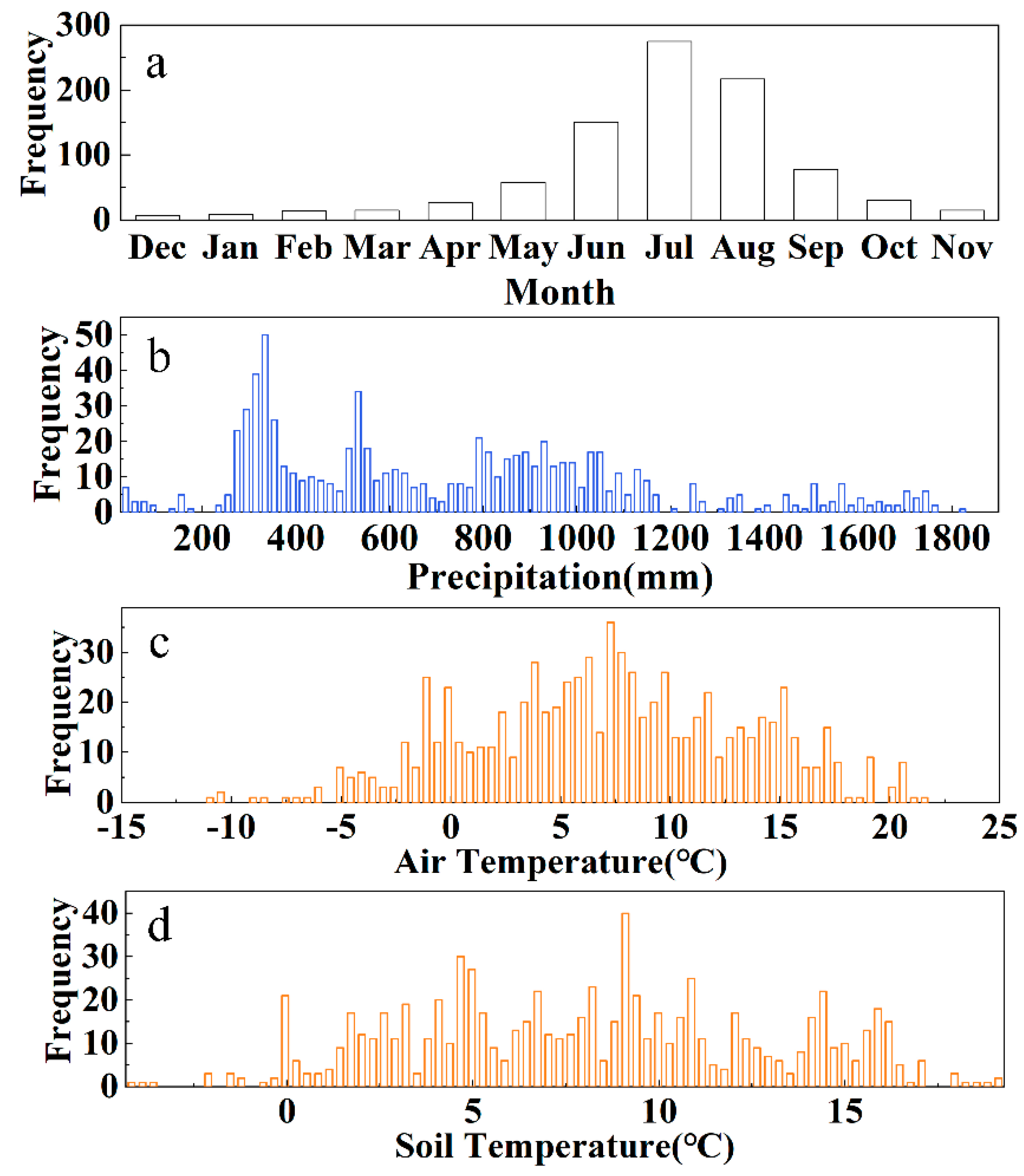
3.2.1. Analysis of Impact Factors

The linear trend [43] over the period 1980 to 2015 for the precipitation and the temperature was calculated for the entire period and each season using the non-parametric Mann-Kendall statistic.
Spatial distribution analysis was performed in a GIS environment through spatial statistical analysis functions [44], as spatial analysis can be used to reveal the patterns of slope geohazard spatial distribution. A grid with a resolution of 0.1° × 0.1° was established in the study area and the area of the study area was calculated accordingly. Slope geohazard coverage areas were defined as the sum of pixel grid areas with slope geohazards identified. We interpolated the spatial meteorological and topographic data with a resolution of 0.1° × 0.1° by using the bilinear interpolation method to generate the spatial distribution of factors such as slope, altitude, rainfall and temperature. The frequency of slope geohazard occurrence in different scopes of each factor was counted, and the correlation between factors and slope geohazards was established.
To explore the distribution variation of slope geohazards with different factors, we divided 36 years into 4 time periods (1980–1989, 1990–1999, 2000–2009, 2010–2015) and compared slope geohazard-covered areas and occurrence seasons in different periods. The correlation statistics of slope geohazards and factors were carried out in different periods.

3.2.2. Subsection

Considering the lag effect of climate on slope geohazards, the meteorological conditions of the season when slope geohazards occur and the season before the slope geohazards occur were analyzed. For example, for summer slope geohazards, the precipitation in spring and summer in the region where the slope geohazards are located should be taken into account; for spring slope geohazards, the precipitation in the preceding winter and spring of the year of slope geohazards should be taken into account. The average precipitation values of June, July and August in the region of a certain summer geohazard were taken as the summer precipitation of the geohazard site. The average precipitation value of March, April and May in the location of the summer geohazards was taken as the spring precipitation of the geohazard site. Then, the mean precipitation of each year’s summer and spring geohazards was obtained, and the precipitation series of the time series were established, to obtain the change trend of summer precipitation and spring precipitation corresponding to the summer geohazards.
In the same way, the summer air temperature, soil temperature, spring air temperature and soil temperature of the summer geohazards were obtained, and the spring precipitation, air temperature, soil temperature and winter precipitation, air temperature and soil temperature of the spring geohazards were obtained. Then, we obtained the trend of them over the time series.

3.2.3. Geohazard Susceptibility Analysis

The random forest model is an integrated learning model based on a decision tree, also known as a simple and efficient artificial intelligence algorithm. Beyond the previously reported geohazard clusters (GCs) distributed on the eastern and southeastern margins of the QTP, slope geohazards occurred above 3000 m in the interior of the QTP and were defined as new geohazard clusters (NGCs). A total of 188 geohazards were collected from the NGCs, and 188 non-geohazard sample points were randomly selected from the QTP, which together constituted 376 total samples. Eighty percent of 376 sample points were randomly selected as the training set of the random forest training calculation, and the remaining 20% were selected as the validation dataset to verify the prediction rate of the results. Altitude, slope and historical meteorological data were selected as the influencing factors in the model. The number of decision trees was set as 500, and the number of parallel simulations was set as 200. Altitude, slope and future meteorological data were brought into the constructed model to obtain the distribution of geohazard susceptibility in 2030, 2060 and 2099. The historical and future meteorological data all included soil temperature in spring, precipitation and soil temperature in summer, and precipitation and soil temperature in winter in 2030, 2060 and 2099.

4. Results

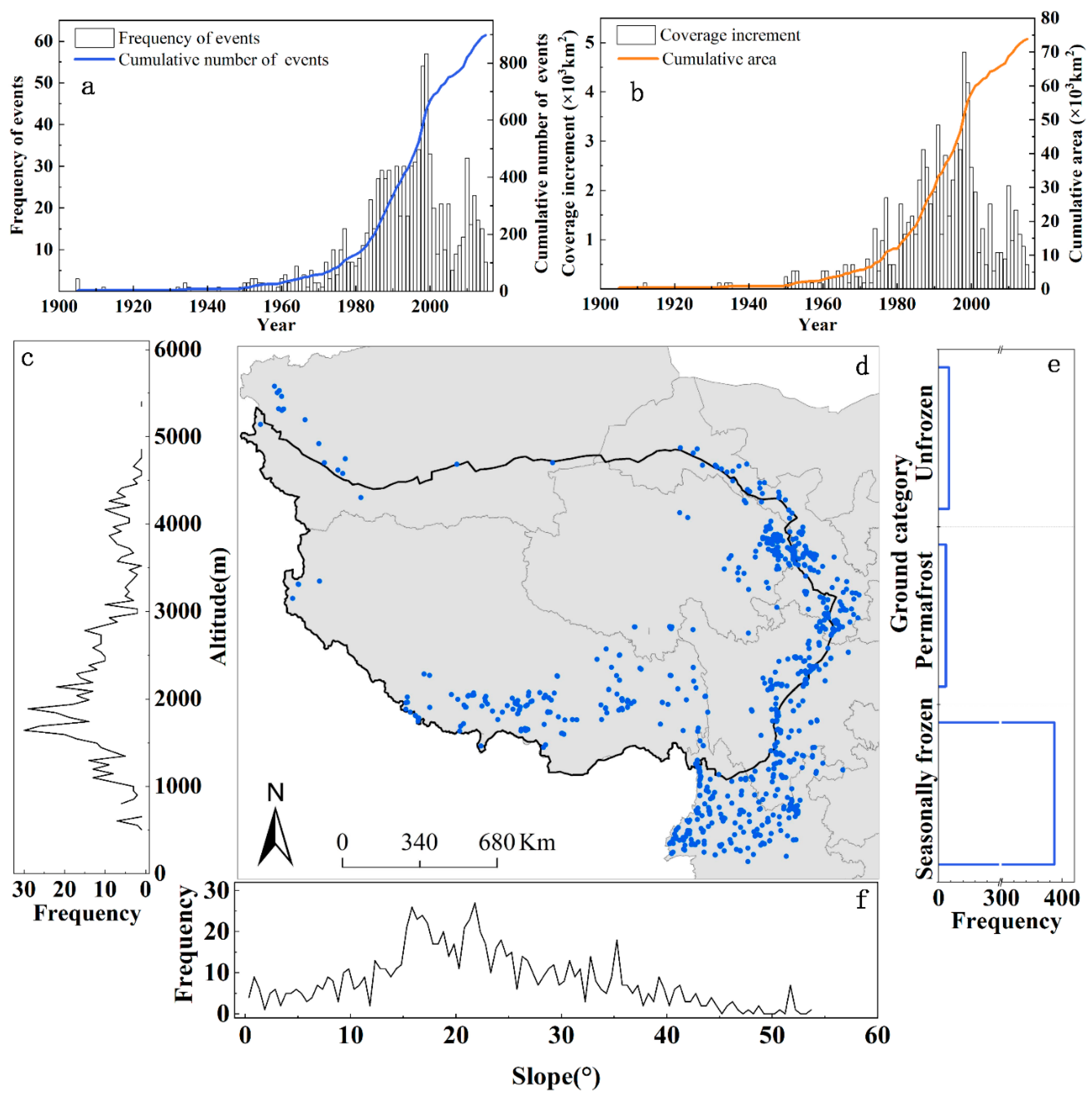
4.1. Disaster-Prone Regions of Slope Geohazards

A total of 897 slope geohazard-covered areas within approximately 73.80 × 10³ km2 were recorded from 1905–2015. A total of 775 slope geohazards were recorded from 1980–2015 with an average frequency of approximately 21.5 times/year (Figure 2a). The numbers and covered areas of slope geohazards have grown rapidly over the past few decades. The slope of the cumulative frequency curve and the cumulative covered area curve after 1980 was larger than that before 1980 and was partly derived from the incomplete records in early decades; furthermore, the frequency and covered area increment in geohazards were the highest in 1998 and 1999 (Figure 2a, b). Notice here that the dataset may slightly underestimate the occurrence of the incidents, for which there are two main reasons:, i.e., the dataset inevitably fails to capture some smaller events, especially in remote mountainous areas [45], and previous event records are not systematic, and data are more difficult to obtain.
Slope geohazards in the study area occurred in slope ranges of 0.36°–53.70° (Figure 2f), and their peak frequency was 13.82°–36.25°. The altitudinal gradient for slope geohazards ranged from 381 m to 5673 m, with peak frequency existing at 1493–1988 m (Figure 2c). The slope geohazard concentrated highly corresponded to the southeastern margins of the QTP, which are the slope geohazard-prone areas with high rates of tectonic processes and intense rainfall in mountain regions [46,47,48,49]. Meanwhile, the slope geohazard distribution also appeared to favor areas of freezing and thawing activities [23,50]. Ninety-three percent of slope geohazards occurred in seasonally frozen regions (Figure 2e), 2.6% were located in permafrost regions and the average altitude was 3818 m. The observed increased temperature and shifted precipitation distribution on the QTP are expected to impact freezing and thawing activities and related slope geohazards.
The occurrence of recorded slope geohazards throughout the year was unevenly distributed, with more events occurring in summer (June–August), followed by autumn (September–November) (Figure 3a). During the period between winter and spring (December–May), the recorded slope geohazard occurrence was low. This pattern reflects the dominant global trigger of slope geohazards, namely, the occurrence of precipitation associated with the Northern Hemisphere summer monsoon [51]. The annual precipitation of slope geohazards presented a bimodal distribution, with the first peak at 254–353 mm and the other peak at 510–550 mm (Figure 3b). In the region with abundant precipitation, slope geohazards are relatively more distributed in the region with annual precipitation of 790–930 mm (Figure 3b). The areas with precipitation in the months of slope geohazards of 50–150 mm are most prone to slope geohazards (Figure S3a). The areas with mean annual air temperatures and soil temperatures ranging from 3.82–9.74 °C (Figure 3c) and 4.67–9.09 °C (Figure 3d) were found to be the most prone to slope geohazards. Overall, slope geohazards, in accordance with these meteorological conditions, were mainly distributed at the eastern edge and southeast of the study area.

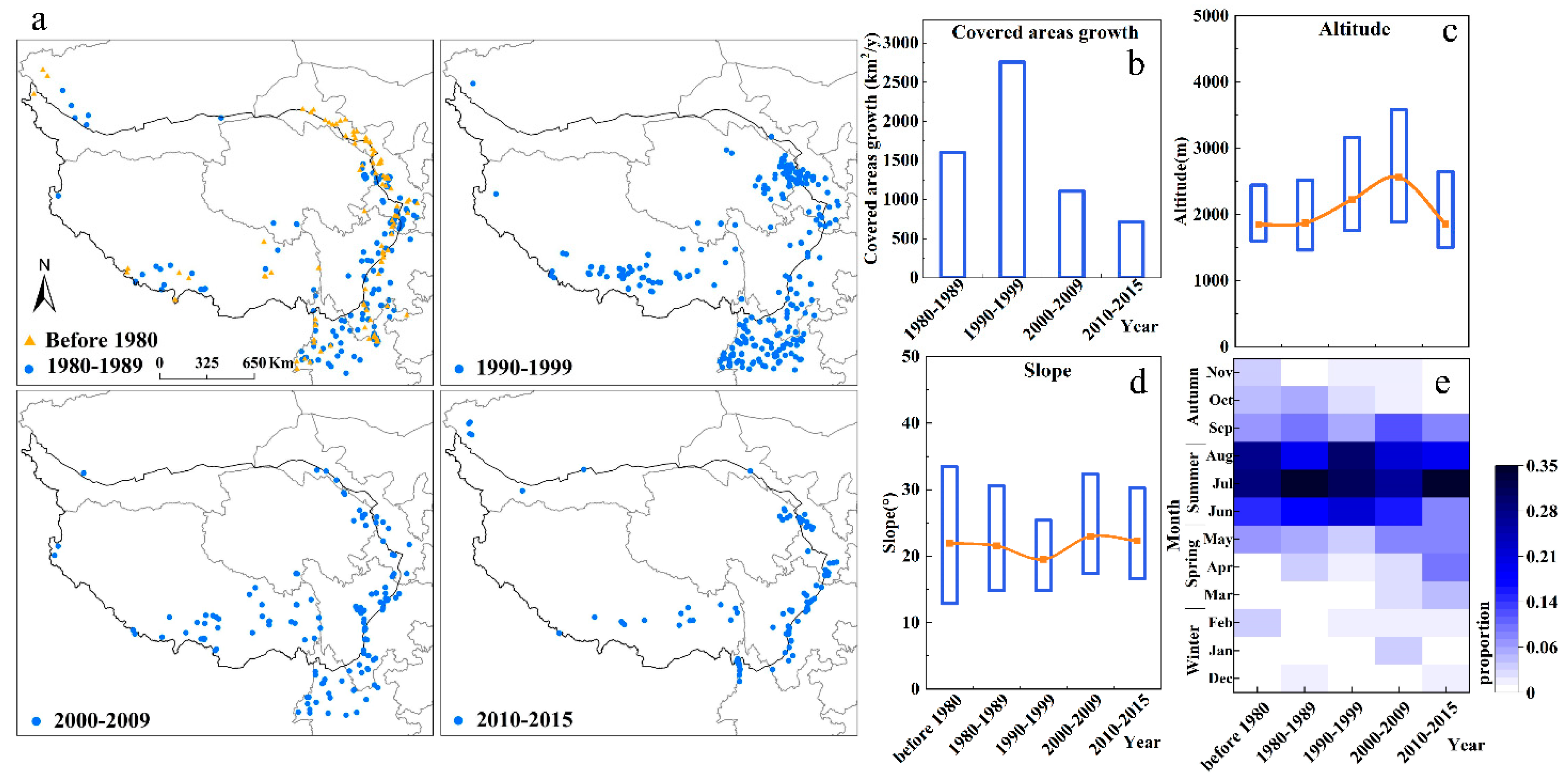
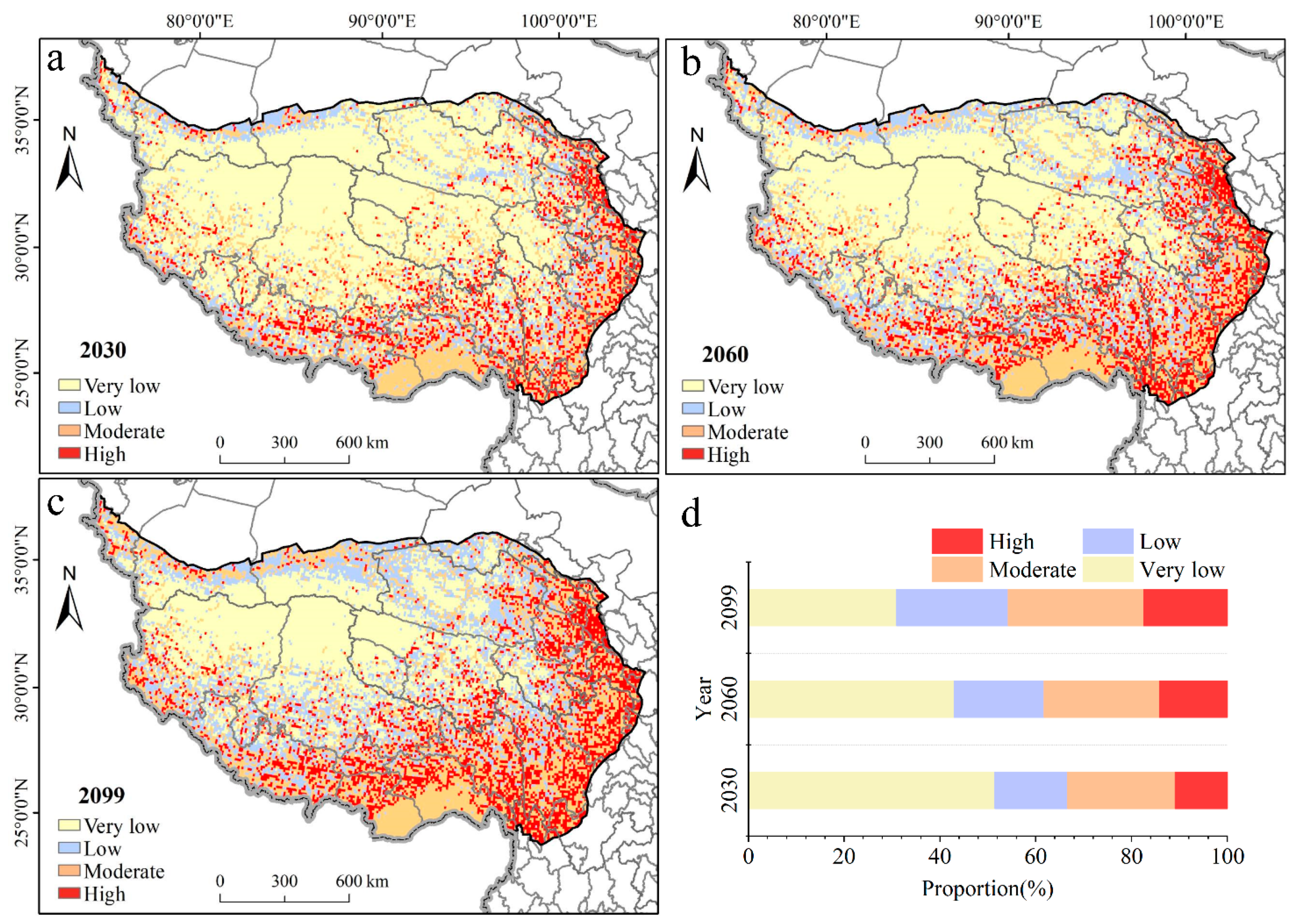
4.2. The Temporal Evolution of Slope Geohazards

We further analyzed the distribution characteristics of slope geohazards in the study area from 1905 to 2015, and explored the changes in slope geohazards with time. For the convenience of comparison, the slope geohazards were divided into five groups according to the time of occurrence (Figure 4a), before 1979 (122 events), 1980–1989 (188 events), 1990–1999 (325 events), 2000–2009 (152 events) and 2010–2015 (110 events). The covered area average annual growth rates of slope geohazards were approximately 1601.7 km2/year for 1980–1989, 2759.9 km2/year for 1990–1999, 1108.9 km2/year for 2000–2009 and 714.6 km2/year for 2010–2015 (Figure 4b). The areal growth rate of slope geohazards from 1990–1999 was 1.7 times as much as from 1980–1989; after 2000, the areal growth rate of slope geohazards was less than from 1990–1999. Slope geohazards spread more widely over time and are likely to become more widespread.
Topographically, slope geohazards vary with time. By 2009, the mean altitude of slope geohazards had increased from 1984 m to 2562 m, with a growth rate of 238 m/10 year (Figure 4c). Then, the mean altitude of the slope geohazards decreased to 1857 m from 2010–2015 because the recorded events in this period were generally located at the lower altitude of the eastern boundary. In contrast, the slope range of slope geohazards remained stable during the study period, with the average slope maintained at 19.53°–22.96° from 1905–2015 (Figure 4b), which indicates that the influence of slope on geohazards in the study area has no obvious change. The altitude of the slope geohazards gradually increases, while the slope gradient varies only slightly. Therefore, the slope is still the most important condition to determine the occurrence of slope geohazards in the study area.
Slope geohazards spread to the spring, although summer and autumn were still the frequent seasons for slope geohazards from 1905–2015 (Figure 4d). Nine percent of slope geohazards occurred in spring before 1980, and 10%, 6%, 14% and 25% of the slope geohazards occurred in spring in the following four periods. The increase in slope geohazards in spring is related to climate change. It was further found that the seasonal variation is more prominent in the area above 2000 m (Figure S4). Before 1980, slope geohazards above 2000 m mostly occurred from May–October and in February, increased to April and December from 1980–1989, expanded to February–November from 1990–1999, expanded to January–November from 2000–2009 and occurred from March–September and in December from 2010–2015. The increase in slope geohazards in high-altitude areas in spring indicates that the driving factors of some slope geohazards in the study area have changed and that the impact of temperature rise is more obvious for slope geohazards.
The increasing frequency of slope geohazards is not only related to precipitation, but also affected by soil temperature. Considering the lagging influence of climate on geohazards, the precipitation and temperature of the previous season should also be taken into account in addition to the precipitation and temperature of the season in which the geohazards occur. The summer monthly precipitation corresponding to the summer geohazards decreased (Figure 5a), while the spring monthly precipitation increased (Figure 5b). The summer and spring soil monthly temperature corresponding to the summer geohazards both decreased (Figure 5c,d). This result suggested that summer geohazards are affected by summer precipitation, spring precipitation, summer soil temperature and spring soil temperature and tend to develop in regions with lower soil temperature in spring, lower soil temperature and less precipitation in summer and that the increase in spring precipitation may lead to geohazards in some areas during summer. The spring and winter soil monthly temperatures corresponding to spring geohazards decreased at a rate of 1.3 °C/10a (Figure 5e,f). This result suggested that spring geohazards are affected by winter and spring soil temperatures and tend to develop in regions with lower soil temperatures in winter and spring. There was no obvious influence on spring geohazards with spring, winter precipitation and air temperature (Figure S5a,b,e,f) and no obvious influence on summer geohazards with spring or summer air temperature (Figure S5c,d).

5. Discussion

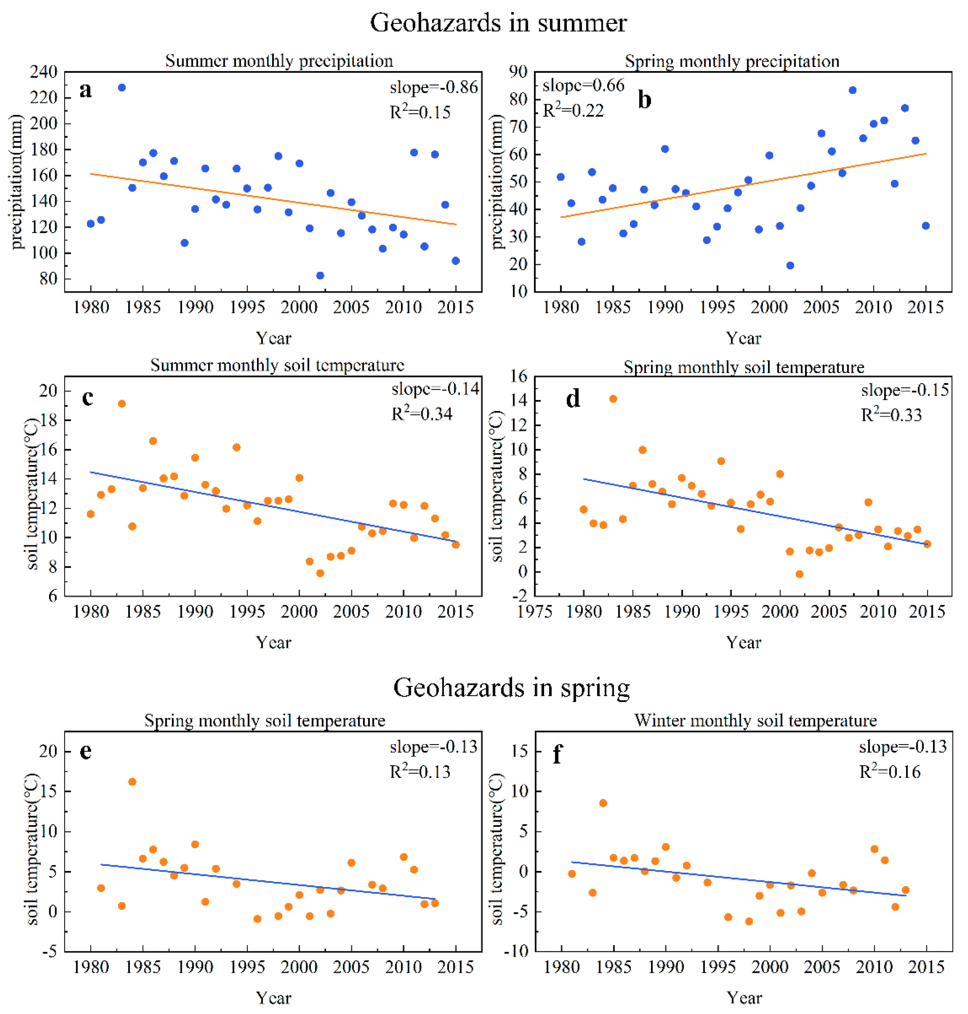
5.1. Locomotion of Slope Geohazards in the QTP and Its Adjacent Regions

The QTP is one of the regions with the most frequent slope geohazards because of its complex geological environments, strong tectonic activity, poor stability of rock slopes and frequent rainstorms [52]. We observed not only the significant growth of slope geohazards but also an accelerating growth rate of scale in past decades, which is consistent with reports that the scale and frequency of slope geohazards in the QTP corridor are increasing [53]. Although such a trend was associated with improving skill in data collection, other field observations also reported an increase in slope failure on the QTP. In the permafrost region of the Qilian Mountains [23] and Fenghuo Mountain [50], slope failure has accelerated, and in the Beiluhe Region on the QTP, the total number of thaw slumps and the total surface area increased significantly [54]. Considering the increased human and economic vulnerability with plateau development, the slope geohazard risk is likely to be higher and requires more attention.
The spatial distribution displayed within the slope geohazard dataset is instructive, with the occurrence of slope geohazards separately concentrated in two altitude ranges. On the one hand, the well-known slope geohazard-prone area along the Himalayan Arc Regions in southeastern edges of the plateau [1,46] and, on the other hand, regions in the central plateau with higher altitudes (above 3000 m) have been suggested to be ever-increasing slope geohazards. The slope geohazards at higher altitudes showed particularity in the occurrence season. Different from traditional slope geohazards, which mainly occur in summer and autumn, the frequency of slope geohazards in high-altitude areas increases significantly in spring [55]. The spatial and temporal migration of slope geohazards both suggested that thaw slump activity is rapidly accelerating in the alpine permafrost regions on the central QTP [23].
It is interesting to find that the mean slope ranges remained steady at 19°–23° within all slope geohazards of different decades. Slope is still the key factor in predicting the slope geohazard risk, and slope size affects the stress distribution inside the slope body and controls the characteristics of surface runoff and groundwater [56]. Statistical results show that 70% of the area is within slope ranges of 13.82°–36.25° on the QTP, covering an area of 7.1 × 10⁵ km2. In higher elevation stands, rising spring temperatures and increasing precipitation will magnify slope geohazard risk [5]. This hypothesis is supported by our results and by short- and long-term studies in the Arctic and other alpine regions. In addition, the prolonged season of high-altitude geological disasters has been affected by climate warming [57].

5.2. Comparison of Two Slope Geohazard Clusters

Observed from the slope geohazard spatial distribution location and elevation variation, we could easily find the migration of slope geohazards. Beyond the previously reported geohazard clusters (GCs) distributed on the eastern and southeastern margins of the QTP, we found that slope geohazards occurred above 3000 m in the interior of the QTP and were defined as new geohazard clusters (NGCs) (Figure 6a). The distribution of GCs and NGCs is shown in Figure 6a. We compared the altitude, slope, season, precipitation, air temperature and soil temperature of the geohazards to illustrate the different driving factors of these two clusters.
In terms of topography, the peak altitude is 1750 m in the GC while it is 4050 m in the NGC, but the frequent slope of the two disaster clusters is 13.82°–36.25°. The influence of slope on geohazards does not vary greatly with region. Summer and autumn are the rainy seasons on the QTP, so June–August is the peak period for the two disaster clusters. However, the proportion of NGCs occurring from May to July is higher than that of GCs, which may be related to the melting of snow and ice in high-altitude areas. In the seasonally frozen area of China, the occurrence of a landslide in summer and autumn is usually induced by rainfall, while in spring, it is caused by the freeze–thaw process [58]. There are two annual rainfall peaks in the GC, one of which is 300–400 mm in the northeastern part of Qinghai Province, which is in the transition zone from the QTP to Loess Plateau with complex terrain [59,60], and the other is 800–1100 mm in Yunnan and the northern part of Sichuan where both terrain and precipitation are conducive to slope geohazard development [29,61,62]. The annual precipitation of the NGC is mostly 300–600 mm. However, there is little difference in the monthly precipitation of the two disaster clusters, most of which are between 70 mm and 120 mm, which suggests that slope geohazards are more common in areas within this monthly precipitation threshold. The different spatial distributions of the two geohazard clusters also mean that there are significant differences in temperature; for example, slope geohazards occur most frequently in NGCs with an average annual temperature of −0.74 °C, while the peak temperature of the frequent geohazard clusters is 7.68 °C in the GC. The air temperature in the months of the geohazards was 6.66 °C in the NGC and 16.91 °C in the GC. Similarly, this difference is also reflected in soil temperature.
We further adopted the random forest model and future climatic data simulated by CMIP5 (RCP 8.5) to obtain the distribution of geohazard susceptibility on the QTP in 2030, 2060 and 2099. Altitude, slope and simulated future air temperature, soil temperature and precipitation were brought into the constructed model. The receiver operating characteristic (ROC) curve of the random forest model in this study is shown in Figure S6, and the area under the curve (AUC) is 0.9702. As the climate changes gradually, slope geohazards will spread over a wider area of the QTP. The proportion of very low-sensitivity areas decreased from 51.44% in 2030 to 42.95% in 2060 and 30.95% in 2099 (Figure 7). The areas of low-sensitivity areas, moderate-sensitivity areas and high-sensitivity areas are increasing. The proportion of highly sensitive areas increased from 10.93% in 2030 to 14.17% in 2060 and 17.48% in 2099. The moderate- and high-sensitivity areas are mainly distributed in the east and south of the QTP. The low-, moderate- and high-sensitivity areas of the QTP are mainly south of 30° N in 2030, extend to the south of 33° N in 2060 and continue to expand to the south of 35° N in 2099. The low-sensitivity region in the northern plateau gradually expands from 37° N inward to 35° N. Geohazards on the QTP will spread from the east and south to the central region.

6. Conclusions

In this study on the QTP, the variation in the spatial and temporal distribution of 897 slope geohazards was assessed. Geographical and meteorological element correlations with the occurrence of slope geohazards were evaluated. By judging the factors that affect changes in slope geohazards, unknown risk areas were forecast. The main findings of our study are as follows.
Ninety-three percent of slope geohazards occurred in seasonally frozen regions, 2.6% were located in permafrost regions and the average altitude was 3818 m. The slope geohazards are mainly concentrated at approximately 2000 m, and the mean altitude spreads from 1984 m to 2562 m. Over time, the altitude of the slope geohazards gradually increases, while the slope gradient varies only slightly. Slope geohazards increased in the spring, especially in areas above 3000 m. The air warming rate and precipitation growth rate at geohazard sites increased gradually, indicating that the increase in spring air temperature and precipitation is an important reason for the increase in spring slope geohazards. Based on the observation of the spatial location, altitude and temperature growth rate of slope geohazards, an NGC appears in the study area, and there is still a possibility of migration under future climate conditions. We estimate that the low-, moderate- and high-sensitivity areas of the QTP are mainly south of 30° N in 2030, extend to the south of 33° N in 2060, continue to expand to the south of 35° N in 2099 and the proportion of high-sensitivity areas increases from 10.93% in 2030 to 14.17% in 2060 and 17.48% in 2099.
However, to explore the specific impact factors of slope geohazards in high-altitude mountain areas, we will further analyze the formation mechanism of slope geohazards with high-resolution datasets of slope geohazards and rigorous long-term records of daily temperature and precipitation in the future [57].

Supplementary Materials

The following are available online at https://0-www-mdpi-com.brum.beds.ac.uk/article/10.3390/su131910488/s1, Figure S1. Spatial distribution of the field survey regions of the QTP; Figure S2. Changes of temperature and precipitation over the QTP, 1980–2015; Figure S3. (a) precipitation, (b) air temperature and (c) soil temperature in the month when the slope geohazards occurred; Figure S4. The proportion of slope geohazards occurring at different elevations in 4 periods; Figure S5. Changes of precipitation and temperature in different seasons of geohazards in different years. (a) spring monthly precipitation in the area of spring geohazards; (b) winter monthly precipitation in the area of spring geohazards; (c) summer monthly air temperature in the area of the summer geohazards; (d) spring monthly air temperature in the area of the summer geohazards; (e) spring monthly air temperature in the area of the spring geohazards; (f) winter monthly air temperature in the area of the spring geohazards; Figure S6. The ROC curve of the random forest model in this study; Table S1. Eight CMIP5 models were used in this study.

Author Contributions

Conceptualization, J.L. (Jifu Liu), L.G.; methodology, Y.J., Z.D.; software, Y.J., Z.D.; validation, all authors; formal analysis, Y.J., L.G., H.Z.; investigation, Y.J., J.L. (Jiaoyang Li); resources, J.L. (Jifu Liu), L.G.; data curation, Y.J., J.L. (Jiaoyang Li), H.Z.; writing—original draft preparation, Y.J.; writing—review and editing, Y.J., L.G.; visualization, Z.D., H.Z.; supervision, L.G.; project administration, J.L. (Jifu Liu), L.G.; funding acquisition, J.L. (Jifu Liu). All authors have read and agreed to the published version of the manuscript.

Funding

This research was funded by the Second Tibetan Plateau Scientific Expedition and Research Program (STEP), Grant No. 2019QZKK0906, and the National Key R&D Program of China, Grant No. 2018YFC1509003.

Institutional Review Board Statement

Not applicable.

Informed Consent Statement

Not applicable.

Data Availability Statement

The data supporting reported results may be made available upon request.

Acknowledgments

We would like to thank the high-performance computing support from the Center for Geodata and Analysis, Faculty of Geographical Science, Beijing Normal University (https://gda.bnu.edu.cn/, accessed on 20 June 2020).

Conflicts of Interest

The authors declare no conflict of interest.

References

  1. Petley, D. Global patterns of loss of life from landslides. Geology 2012, 40, 927–930. [Google Scholar] [CrossRef]
  2. Andres, N.; Badoux, A. The Swiss flood and landslide damage database: Normalisation and trends. J. Flood Risk Manag. 2018, 12, e12510. [Google Scholar] [CrossRef] [Green Version]
  3. Haque, U.; Blum, P.; da Silva, P.F.; Andersen, P.; Pilz, J.; Chalov, S.R.; Malet, J.-P.; Auflič, M.J.; Andres, N.; Poyiadji, E.; et al. Fatal landslides in Europe. Landslides 2016, 13, 1545–1554. [Google Scholar] [CrossRef]
  4. Saez, J.L.; Corona, C.; Stoffel, M.; Berger, F. Climate change increases frequency of shallow spring landslides in the French Alps. Geology 2013, 41, 619–622. [Google Scholar] [CrossRef]
  5. Stoffel, M.; Tiranti, D.; Huggel, C. Climate change impacts on mass movements—Case studies from the European Alps. Sci. Total Environ. 2014, 493, 1255–1266. [Google Scholar] [CrossRef]
  6. Vergara Dal Pont, I.; Moreiras, S.M.; Santibañez Ossa, F.; Araneo, D.; Ferrando, F. Debris flows triggered from melt of seasonal snow and ice within the active layer in the semi-arid Andes. Permafr. Periglac. Process. 2019, 31, 57–68. [Google Scholar] [CrossRef]
  7. Schar, C.; Vidale, P.L.; Luthi, D.; Haberli, C.F.; Liniger, M.A.; Appenzeller, C. The role of increasing temperature variability in European summer heatwaves. Nature 2004, 427, 332–336. [Google Scholar] [CrossRef]
  8. Kääb, A.; Chiarle, M.; Raup, B.; Schneider, C. Climate change impacts on mountain glaciers and permafrost. Glob. Planet. Chang. 2007, 56, vii–ix. [Google Scholar] [CrossRef]
  9. Noetzli, J.; Huggel, C.; Hoelzle, M.; Haeberli, W. GIS-based modelling of rock-ice avalanches from Alpine permafrost areas. Comput. Geosci. 2006, 10, 161–178. [Google Scholar] [CrossRef] [Green Version]
  10. Davies, M.C.R.; Hamza, O.; Harris, C. The effect of rise in mean annual temperature on the stability of rock slopes containing ice-filled discontinuities. Permafr. Periglac. Process. 2001, 12, 137–144. [Google Scholar] [CrossRef]
  11. Chiarle, M.; Mortara, G. Geomorphological impact of climate change on alpine glacial and periglacialareas. Conf. Proc. 2008, 2, 111–122. [Google Scholar]
  12. Qiu, H.; Cui, Y.; Hu, S.; Yang, D.; Pei, Y.; Yang, W. Temporal and spatial distributions of landslides in the Qinba Mountains, Shaanxi Province, China. Geomat. Nat. Hazards Risk 2019, 10, 599–621. [Google Scholar] [CrossRef]
  13. Climate Change Could Trigger More Landslides in High Mountain Asia. Available online: https://climate.nasa.gov/news/2951/climate-change-could-trigger-more-landslides-in-high-mountain-asia/ (accessed on 5 July 2021).
  14. Tokashiki, N.; Aydan, O. Kita-Uebaru natural rock slope failure and its back analysis. Environ. Earth Sci 2011, 62, 25–31. [Google Scholar] [CrossRef]
  15. Tonini, M.; Cama, M. Spatio-temporal pattern distribution of landslides causing damage in Switzerland. Landslides 2019, 16, 2103–2113. [Google Scholar] [CrossRef]
  16. Khan, M.S.; Hossain, S.; Ahmed, A.; Faysal, M. Investigation of a shallow slope failure on expansive clay in Texas. Eng. Geol. 2017, 219, 118–129. [Google Scholar] [CrossRef]
  17. Winter, M.G.; Dixon, N.; Wasowski, J.; Dijkstra, T.A. Introduction to land-use and climate change impacts on landslides. Q. J. Eng. Geol. Hydrogeol. 2010, 43, 367–370. [Google Scholar] [CrossRef]
  18. Papathoma-Köhle, M. Vulnerability curves vs. vulnerability indicators: Application of an indicator-based methodology for debris-flow hazards. Nat. Hazards Earth Syst. Sci. 2016, 16, 1771–1790. [Google Scholar] [CrossRef] [Green Version]
  19. Jia, H.; Chen, F.; Pan, D. Disaster Chain Analysis of Avalanche and Landslide and the River Blocking Dam of the Yarlung Zangbo River in Milin County of Tibet on 17 and 29 October 2018. Int. J. Environ. Res. Public Health 2019, 16, 4707. [Google Scholar] [CrossRef] [PubMed] [Green Version]
  20. Li, X.; Cheng, G.; Jin, H.; Kang, E.; Che, T.; Jin, R.; Wu, L.; Nan, Z.; Wang, J.; Shen, Y. Cryospheric change in China. Glob. Planet. Chang. 2008, 62, 210–218. [Google Scholar] [CrossRef]
  21. Yao, T.; Xue, Y.; Chen, D.; Chen, F.; Thompson, L.; Cui, P.; Koike, T.; Lau, W.K.-M.; Lettenmaier, D.; Mosbrugger, V.; et al. Recent Third Pole’s Rapid Warming Accompanies Cryospheric Melt and Water Cycle Intensification and Interactions between Monsoon and Environment: Multidisciplinary Approach with Observations, Modeling, and Analysis. Bull. Am. Meteorol. Soc. 2019, 100, 423–444. [Google Scholar] [CrossRef]
  22. Hao, J.; Zhao, L.; Li, R.; Xie, C.; Wu, T.; Wu, X.; Hu, G.; Zou, D.; Zhu, X.; Ni, J.; et al. Investigation of a Small Landslide in the Qinghai-Tibet Plateau by InSAR and Absolute Deformation Model. Remote Sens. 2019, 11, 2126. [Google Scholar] [CrossRef] [Green Version]
  23. Mu, C.; Shang, J.; Zhang, T.; Fan, C.; Wang, S.; Peng, X.; Zhong, W.; Zhang, F.; Mu, M.; Jia, L. Acceleration of thaw slump during 1997–2017 in the Qilian Mountains of the northern Qinghai-Tibetan plateau. Landslides 2020, 17, 1051–1062. [Google Scholar] [CrossRef]
  24. Gao, Y.J.; Cheng, N.S.; Hu, G.S.; Deng, M.S. Temporal and Spatial Coupling Relationship Between Debris Flow and El Nino-La Nina Event in Southwest China. J. Yangtze River Sci. Res. Inst. 2019, 36, 43–48. [Google Scholar] [CrossRef]
  25. Wei, R.; Zeng, Q.; Davies, T.; Yuan, G.; Wang, K.; Xue, X.; Yin, Q. Geohazard cascade and mechanism of large debris flows in Tianmo gully, SE Tibetan Plateau and implications to hazard monitoring. Eng. Geol. 2018, 233, 172–182. [Google Scholar] [CrossRef]
  26. Yang, Y.; Wu, Q.; Jin, H.; Wang, Q.; Huang, Y.; Luo, D.; Gao, S.; Jin, X. Delineating the hydrological processes and hydraulic connectivities under permafrost degradation on Northeastern Qinghai-Tibet Plateau, China. J. Hydrol. 2019, 569, 359–372. [Google Scholar] [CrossRef]
  27. Zou, D.; Zhao, L.; Sheng, Y.; Chen, J.; Hu, G.; Wu, T.; Wu, J.; Xie, C.; Wu, X.; Pang, Q.; et al. A new map of permafrost distribution on the Tibetan Plateau. Cryosphere 2017, 11, 2527–2542. [Google Scholar] [CrossRef] [Green Version]
  28. Chen, D.; Xu, B.; Yao, T.; Guo, Z.; Cui, P.; Chen, F.; Zhang, R.; Zhang, X.; Zhang, Y.; Fan, J.; et al. Assessment of past, present and future environmental changes on the Tibetan Plateau. Chin. Sci Bull. 2015, 60, 3025–3035. [Google Scholar] [CrossRef]
  29. Yang, F.; Wang, W.; Wang, H.; Li, X.; Jiang, W. The Distribution Characters of the Stratospheric Zonal Mean Temperature and Water Vapor during 1979–2011. Plateau Mt. Meteorol. Res. 2016, 36, 63–67. [Google Scholar]
  30. Zhang, Y.; Guo, C.; Yao, X.; Yang, Z.; Wu, R.; Du, G. Research on the Geohazard Effect of Active Fault on the Eastern Margin of the Tibetan Plateau. Acta Geosci. Sin. 2016, 37, 277–286. [Google Scholar] [CrossRef]
  31. Zhou, J.; Cui, P.; Hao, M. Comprehensive analyses of the initiation and entrainment processes of the 2000 Yigong catastrophic landslide in Tibet, China. Landslides 2016, 13, 39–54. [Google Scholar] [CrossRef]
  32. Cui, P.; Chen, R.; Xiang, L.; Su, F. Risk analysis of mountain hazards in Tibetan Plateau under the global warming. Progress. Inquisitiones De Mutat. Clim. 2014, 10, 103–109. [Google Scholar] [CrossRef]
  33. Deng, J.; Dai, F.; Wen, B. Catastrophic mechanisms and risk control of major landslides in Tibetan Plateau. Adv. Eng. Sci. 2019, 52, 1–8. [Google Scholar] [CrossRef]
  34. Dong, A.; Wen, K. Chinese Meteorological Disasters Ceremony (Gansu Volume); China Meteorological Press: Beijing, China, 2005. (In Chinese) [Google Scholar]
  35. Liu, G.; Wen, K. Chinese Meteorological Disasters Ceremony (Tibet Volume); China Meteorological Press: Beijing, China, 2008. (In Chinese) [Google Scholar]
  36. Liu, J.; Wen, K. Chinese Meteorological Disasters Ceremony (Yunnan Volume); China Meteorological Press: Beijing, China, 2006. (In Chinese) [Google Scholar]
  37. Shi, Y.; Wen, K. Chinese Meteorological Disasters Ceremony (Xinjiang Volume); China Meteorological Press: Beijing, China, 2006. (In Chinese) [Google Scholar]
  38. Wang, X.; Wen, K. Chinese Meteorological Disasters Ceremony (Qinghai Volume); China Meteorological Press: Beijing, China, 2007. (In Chinese) [Google Scholar]
  39. Zhan, Z.; Wen, K. Chinese Meteorological Disasters Ceremony (Sichuan Volume) (in Chinese); China Meteorological Press: Beijing, China, 2006. (In Chinese) [Google Scholar]
  40. Liu, C.; Liu, X.; Chen, Q.; Gao, W. Impact of DEM spatial resolution on landslide extraction using object-oriented methods. Remote Sens. Technol. Appl. 2014, 29, 631–638. [Google Scholar]
  41. Taylor, K.E.; Stouffer, R.J.; Meehl, G.A. An Overview of CMIP5 and the Experiment Design. Bull. Am. Meteorol. Soc. 2012, 93, 485–498. [Google Scholar] [CrossRef] [Green Version]
  42. You, Q.; Min, J.; Kang, S. Rapid warming in the Tibetan Plateau from observations and CMIP5 models in recent decades. Int. J. Climatol. 2016, 36, 2660–2670. [Google Scholar] [CrossRef]
  43. Sen, P.K. Estimates of the Regression Coefficient Based on Kendall’s Tau. J. Am. Stat. Assoc. 1968, 63, 1379–1389. [Google Scholar] [CrossRef]
  44. Zhao, B.; Wang, Y.; Chen, M.; Luo, Y.; Liang, R.; Li, J. Typical characteristics of large-scale landslides in the transition belt between the Qinghai-Tibet Plateau and the Loess Plateau. Arab. J. Geosci. 2019, 12, 470. [Google Scholar] [CrossRef]
  45. Sepúlveda, S.A.; Petley, D.N. Regional trends and controlling factors of fatal landslides in Latin America and the Caribbean. Nat. Hazards Earth Syst. Sci. 2015, 15, 1821–1833. [Google Scholar] [CrossRef] [Green Version]
  46. Bai, S.; Lu, P.; Thiebes, B. Comparing characteristics of rainfall- and earthquake-triggered landslides in the Upper Minjiang catchment, China. Eng. Geol. 2020, 268, 105518. [Google Scholar] [CrossRef]
  47. Huang, R. Some catastrophic landslides since the twentieth century in the southwest of China. Landslides 2009, 6, 69–81. [Google Scholar] [CrossRef]
  48. Bai, Y.; Ni, H.; Ge, H. Advances research progress on geohazard effect of active faults on the southeastern margin of the Tibetan Plateau. J. Geomech. 2019, 25, 1116–2019. [Google Scholar] [CrossRef]
  49. Luo, F.; Ren, G.; Li, H.; Li, Y. Development rules of landslides and collapses along provincial highway S216 in Sichuan. J. Yangtze River Sci. Res. Inst. 2019, 36, 37–41. [Google Scholar]
  50. Ma, W.; Niu, F.; Satoshi, A.; Jin, D. Slope instability phenomena in permafrost regions of Qinghai-Tibet Plateau, China. Landslides 2006, 3, 260–264. [Google Scholar] [CrossRef]
  51. Petley, D.N. On the impact of climate change and population growth on the occurrence of fatal landslides in South, East and SE Asia. Q. J. Eng. Geol. Hydrogeol. 2010, 43, 487–496. [Google Scholar] [CrossRef]
  52. Cao, J.; Zhang, Z.; Du, J.; Zhang, L.; Song, Y.; Sun, G. Multi-geohazards susceptibility mapping based on machine learning—A case study in Jiuzhaigou, China. Nat. Hazards 2020, 102, 851–871. [Google Scholar] [CrossRef]
  53. Niu, F.; Luo, J.; Lin, Z.; Fang, J.; Liu, M. Thaw-induced slope failures and stability analyses in permafrost regions of the Qinghai-Tibet Plateau, China. Landslides 2016, 13, 55–65. [Google Scholar] [CrossRef]
  54. Luo, J.; Niu, F.; Lin, Z.; Liu, M.; Yin, G. Recent acceleration of thaw slumping in permafrost terrain of Qinghai-Tibet Plateau: An example from the Beiluhe Region. Geomorphology 2019, 341, 79–85. [Google Scholar] [CrossRef]
  55. Lin, Q.; Wang, Y.; Glade, T.; Zhang, J.; Zhang, Y. Assessing the spatiotemporal impact of climate change on event rainfall characteristics influencing landslide occurrences based on multiple GCM projections in China. Clim. Chang. 2020, 162, 761–779. [Google Scholar] [CrossRef]
  56. Kui, Z. The study of geological emergence of susceptible division in Yunan district-based on Arcgis. J. Geol. Hazards Environ. Preserv. 2020, 31, 38–42. [Google Scholar]
  57. Stoffel, M.; Mendlik, T.; Schneuwly-Bollschweiler, M.; Gobiet, A. Possible impacts of climate change on debris-flow activity in the Swiss Alps. Clim. Chang. 2013, 122, 141–155. [Google Scholar] [CrossRef] [Green Version]
  58. Li, T.; Li, P.; Wang, H. Forming Mechanism of Landslides in the Seasonal Frozen Loess Region in China. In Landslides in Cold Regions in the Context of Climate Change; Springer International Publishing: New York, NY, USA, 2014; pp. 41–51. [Google Scholar]
  59. Zhao, D.; Lancuo, Z.; Hou, G.; Xu, C.; Li, W. Assessment of geological disaster susceptibility in the Hehuang Valley of Qinghai Province. J. Geomech. 2021, 27, 84–95. [Google Scholar]
  60. Wei, G.; Yin, Z.; Shi, L.; Ma, W.; Cui, X. Zoning of geological disasters of Hualong county in Qinghai province. Chin. J. Geol. Hazard. Control. 2013, 24, 86–92. [Google Scholar] [CrossRef]
  61. Wang, J.; Tian, T.; Zou, Y.; Wang, J.; Fu, X. Mechanical Mechanism of the Rainfall-inducing Deposit Slope Failure in Yunnan Region. J. Water Resour. Archit. Eng. 2020, 18, 204–227. [Google Scholar]
  62. He, R.; Lin, Q.; Wang, Y.; Song, C. Factors and high risk area analysis of geological hazards in Yunnan. J. Catastrophology 2015, 30, 208–213. [Google Scholar] [CrossRef]
Figure 1. Overview of the study area. (a) Slope gradient; (b) elevation; (c) land use classification; (d) mean annual air temperature; (e) mean annual soil temperature; (f) mean annual precipitation.
Sustainability 13 10488 g001
Figure 2. Slope geohazard distributions in the study area, 1905-2015. (a) Slope geohazard frequency per year and cumulative frequency (blue curve); (b) covered area of the slope geohazards per year and cumulative covered area (orange curve); (c) frequency of slope geohazards at different altitudes; (d) spatial distribution of slope geohazards in the study area; (e) frequency of slope geohazards in permafrost regions; (f) frequency of slope geohazards at different slopes.
Sustainability 13 10488 g002
Figure 3. The temporal and meteorological characteristics of slope geohazard distributions in the study area. (a) Monthly frequency of slope geohazards; (b) annual precipitation at slope geohazard sites; (c) average annual air temperature at slope geohazard sites; (d) average annual soil temperature at slope geohazard sites.
Sustainability 13 10488 g003
Figure 4. Slope geohazard change in different periods. (a) Spatial distribution of slope geohazards in different periods (the orange triangles represent geohazard sites before 1980, and the blue circles represent geohazard sites from 1980–1989, 1990–1999, 2000–2009, and 2010-2015); (b) the growth rate of the covered area; (c) the altitude of slope geohazards in different periods (the blue box represents 25%–75% of altitude range in geohazard sites, and the orange curve represents the variation in average altitude); (d) the slope gradient of slope geohazards in different periods (the blue box represents 25%–75% of slope range in geohazard sites, and the orange curve represents the variation in average slope); (e) the monthly proportion of slope geohazards in different periods.
Sustainability 13 10488 g004
Figure 5. Changes in precipitation and temperature in different seasons of geohazards in different years. (a) Summer monthly precipitation in the area of summer geohazards; (b) spring monthly precipitation in the area of summer geohazards; (c) summer monthly soil temperature in the area of the summer geohazards; (d) spring monthly soil temperature in the area of the summer geohazards; (e) spring monthly soil temperature in the area of the spring geohazards; (f) winter monthly soil temperature in the area of the spring geohazards.
Sustainability 13 10488 g005
Figure 6. Comparison of the characteristics of new slope geohazard clusters (NGCs) and previously reported geohazard clusters (GCs). (a) Elevation-geohazard frequency curve comparison (blue curve refers to NGC, orange curve refers to GC); (b) slope-geohazard frequency curve comparison; (c) the comparison of the two clusters spatial distributions; (d) month-geohazard frequency curve comparison; (e) precipitation-geohazard frequency curve comparison (the solid line refers to the annual precipitation of geohazards, while the dotted line refers to the monthly precipitation of geohazards); (f) air temperature-geohazard frequency curve comparison (the solid line refers to the annual temperature of geohazards, while the dotted line refers to the monthly temperature of geohazards); (g) soil temperature-geohazard frequency curve comparison.
Sustainability 13 10488 g006
Figure 7. The slope geohazard sensitivity map area proportion of different grades. (a) Slope geohazard sensitivity map in 2030; (b) slope geohazard sensitivity map in 2060; (c) slope geohazard sensitivity map in 2099; (d) area variation across the sensitivity grades in different periods.
Sustainability 13 10488 g007
Publisher’s Note: MDPI stays neutral with regard to jurisdictional claims in published maps and institutional affiliations.

