
Ecosystem Services Evaluation of Nature-Based Solutions with the Help of Citizen Scientists

 ,
,
Abstract
:1. Introduction
2. Materials and Methods
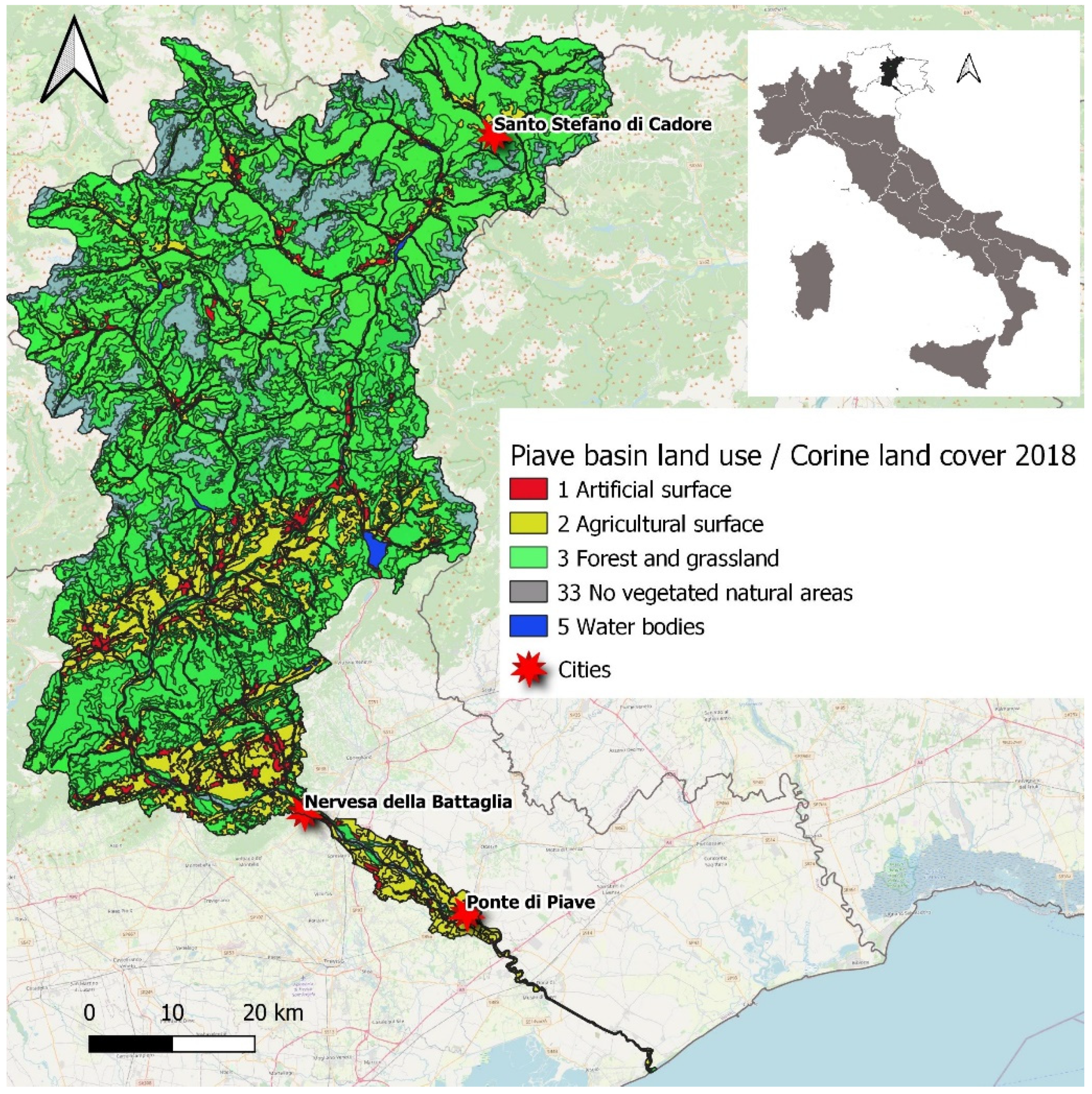
2.1. Study Site
2.2. Model
2.3. Data Sources for Model Development and Validation
- A digital elevation model (DEM), of 20 m resolution, obtained from the Italian ISPRA (Istituto Superiore per la Protezione e la Ricerca Ambientale) [75], was corrected to fill hydrological sinks and checked with the digital watercourse network to ensure routing along the specific watercourse, using QGIS 3.12 (https://www.qgis.org, accessed on 24 March 2021);
- LULC raster data (2018) were obtained from Corine Land Use Land Cover IV Level for Italy [76], at a 100 m resolution;
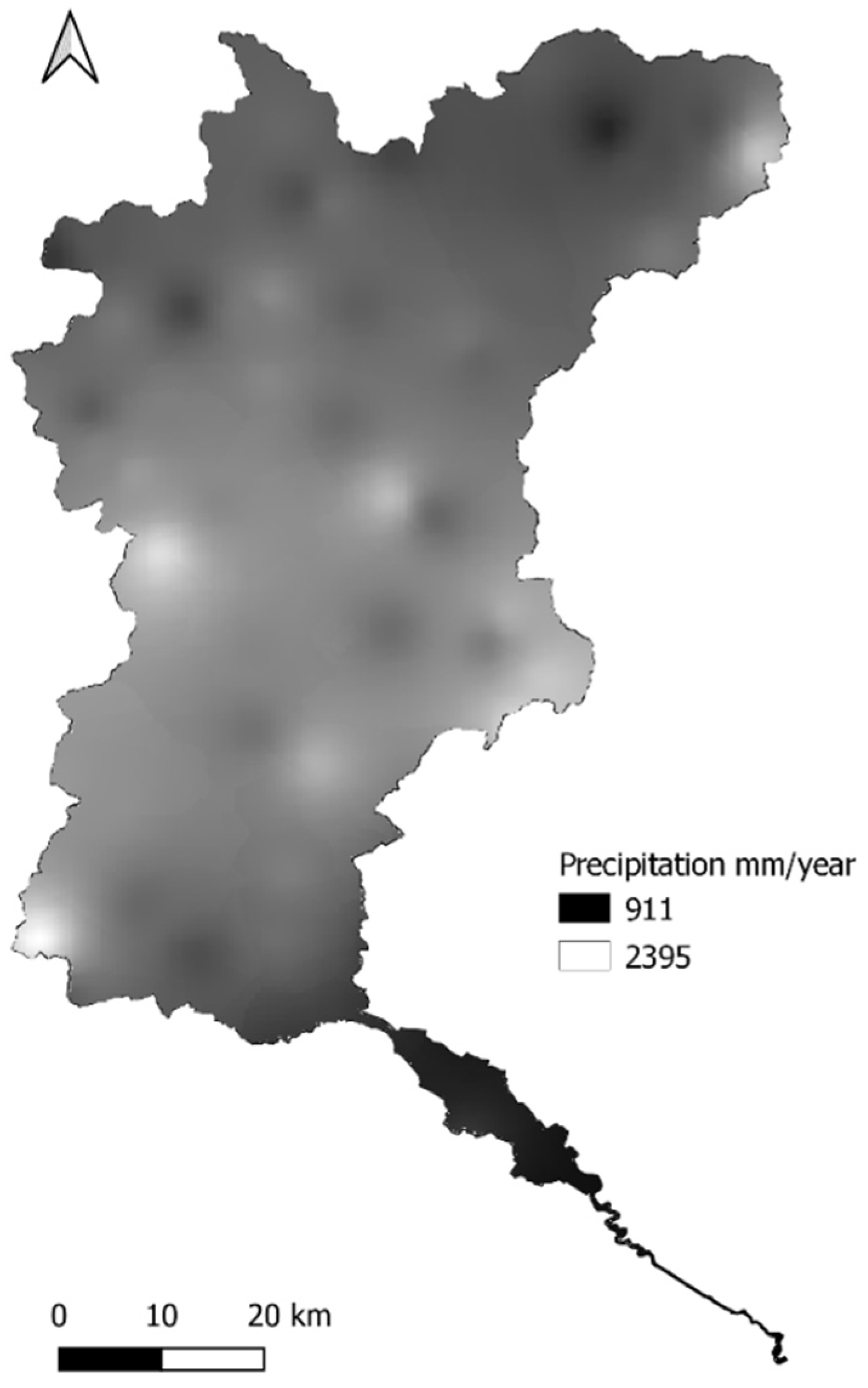
- Nutrient runoff proxies were based on raster precipitation data from 2018, provided by the river catchment authorities (Autorità di Bacino Distrettuale delle Alpi Orientali) at a 20 m resolution. These raster data were interpolated using an inverse distance weighting of information from 72 stations;
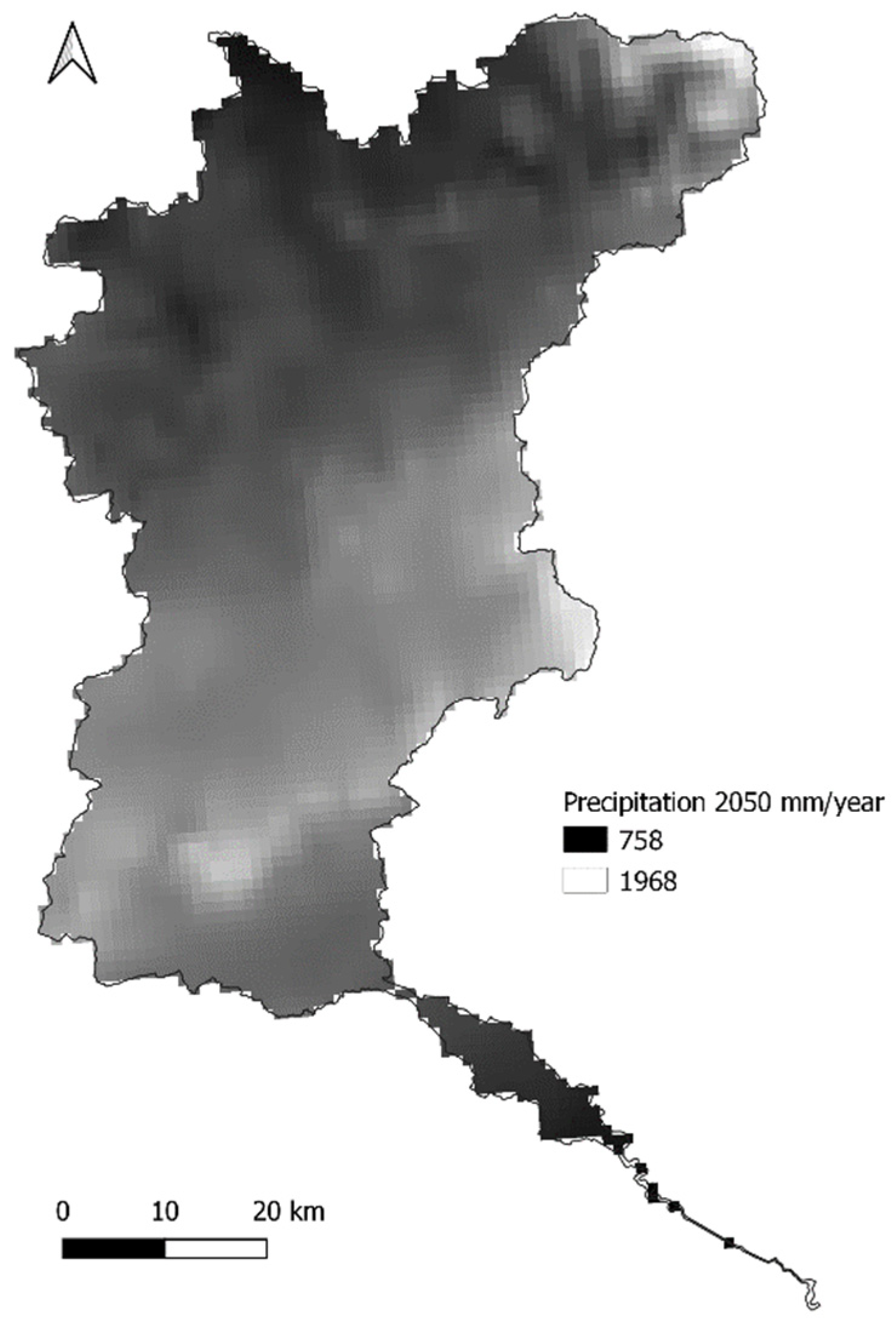
- Future Nutrient runoff proxies were based on precipitation estimates for 2050 by Deszi e al. [77] with high-resolution gridded surfaces at 1 km cell size developed in an Albers Equal Area Conic projection for Europe. Vector delineation of the watershed was obtained from the geoportal of ARPAV, relative to the Water Protection Plan 2015 (Piano di Tutela delle Acque) [78];
- The threshold value for flow accumulation, the number of upriver cells that flow into a cell before it is considered part of a river, was set to 1000, after several tests to compare the river layer output of the model to the measured river network data [79].
- Borselli’s k for the connection of the surrounding land to the river with respect to the ratio of nutrients reaching the river was set to 2 [80];
- The nutrient (N and P) sources associated with each LULC class (kg ha−1 y−1) were based on 2001 data from ARPAV for Corine LULC classes 111–243 (artificial surfaces and agricultural areas) for each municipality and scaled for relative population changes in 2020. For Corine LULC classes 3112–523 (forest and semi-natural areas and water bodies), nutrient load data were obtained from the ARPAV relative to 2018 [81]. The proportion of subsurface N, a floating-point between 0 and 1, was obtained by intersecting a Corine LULC 2018 vector layer with a groundwater infiltration potential layer [82]. In order to obtain the proportion of subsurface N, the groundwater N infiltration risk potential was compared to the protective soil capacity layer [83,84] (Table 1). For each LULC, the final subsurface_N value is weighted for the % of Corine LULC polygons per risk class and calculated as the median of all level 1 Corine LULC classes (i.e., all urban classes, all agricultural classes, all forest classes, etc.) (Table 1).
- Nitrate and phosphate concentrations were obtained through regulatory (ARPAV) and CS measurements. Quarterly ARPAV monitoring of total nitrogen and total phosphorus in four stations in the upper catchment and four sites in the lower catchment were used for model development. Data are available online at www.arpa.veneto.it/dati-ambientali/open-data/idrosfera/corsi-dacqua (accessed on 3 August 2021);
- Trained citizen scientists used the FreshWater Watch method (https://freshwaterwatch.thewaterhub.org/content/freshwater-watch-how-guide, accessed on 3 August 2021) to determine nitrate and phosphate in 12 sites in the lower catchment for model validation. Online and video training followed the standard training program of this global citizen science project [88]. Thirty-five participants in the lower catchment of Piave from Ponte di Piave to the sea collected both observation data (color, presence of algae, etc.) and semi-quantitative measurements of water quality (nitrate, phosphate, nephelometric turbidity) [89,90]. Nitrate (NO3-N) and phosphate (PO4-P) were measured in closed plastic tubes, which are designed to mix a fixed volume of water with reagents to produce increasing color values (peak absorption at 540 nm) with increasing concentration. PO4-P concentrations were estimated colourimetrically using inosine enzymatic reactions in seven specific ranges from 0.02 mg L−1 to 1.0 mg L−1 PO4-P (<0.02, 0.02–0.05, 0.05–0.1, 0.1–0.2, 0.2–0.5, 0.5–1.0, <1.0 mg/L) [91]. Nitrate–nitrogen concentrations were estimated colourimetrically using N-(1-napthyl)-ethylenediamine [92], in seven specific ranges from 0.2 mg L−1 to 10 mg L−1 NO3-N (<0.2, 0.2–0.5, 0.5–1.0, 1.0–2.0, 2.0–5.0, 5–10, >10 mg/L). The median values for each classification were used to allow for quantitative analysis. During the measurements, geo-location and time were recorded automatically using the FreshWater Watch app and transferred to the online database after validation (https://freshwaterwatch.thewaterhub.org/, accessed on 3 august 2021). Once entered, all data underwent quality control by project leaders and citizen scientists.
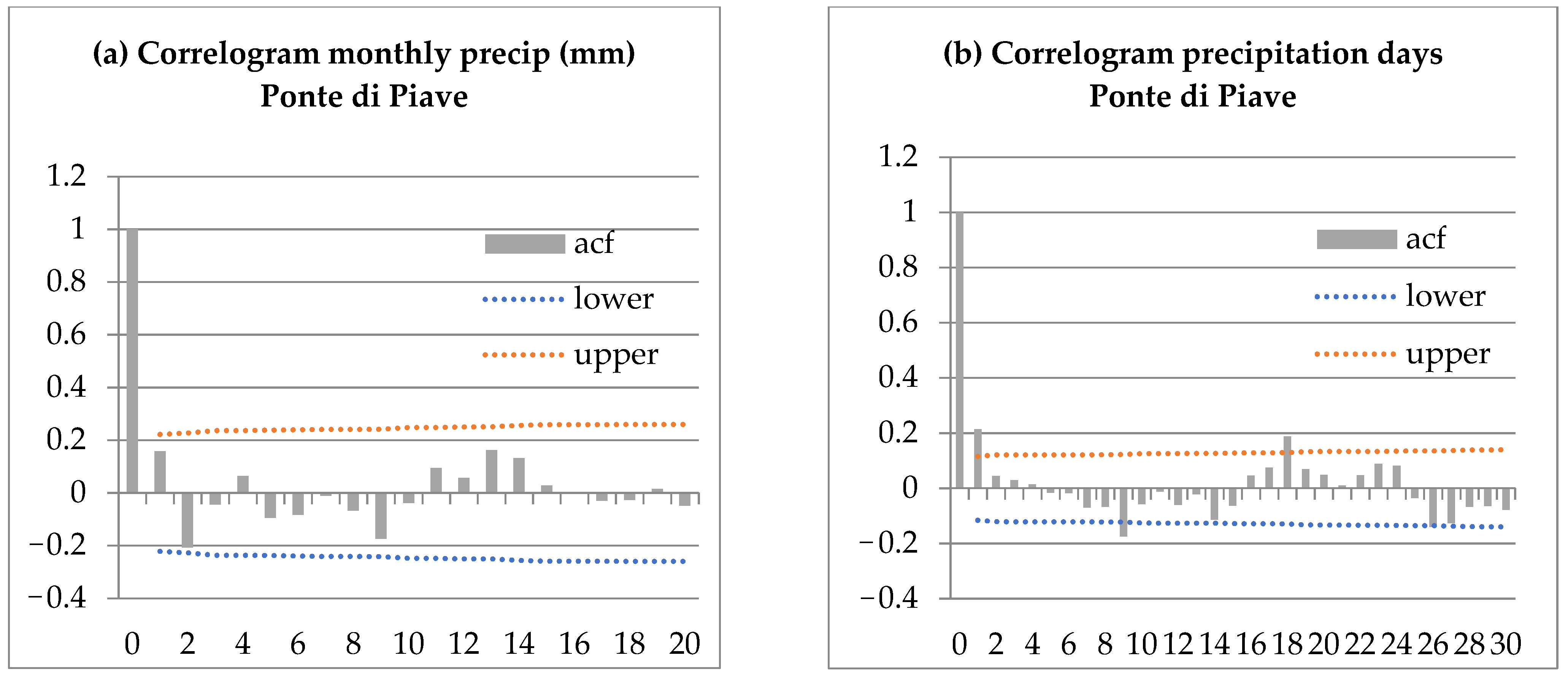
2.4. Climatic Variations
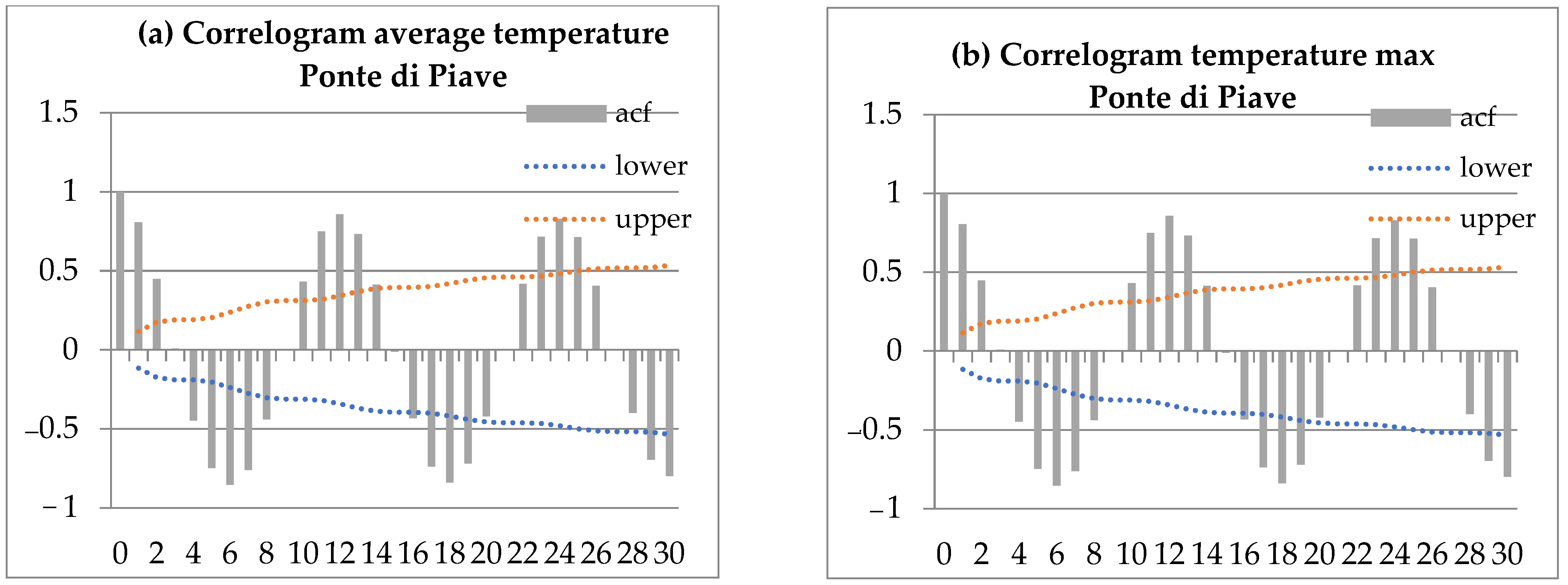
- ARPAV data of Ponte di Piave station (1995–2018) lower catchment, Santo Stefano di Cadore station (1998–2018) upper catchment [93];
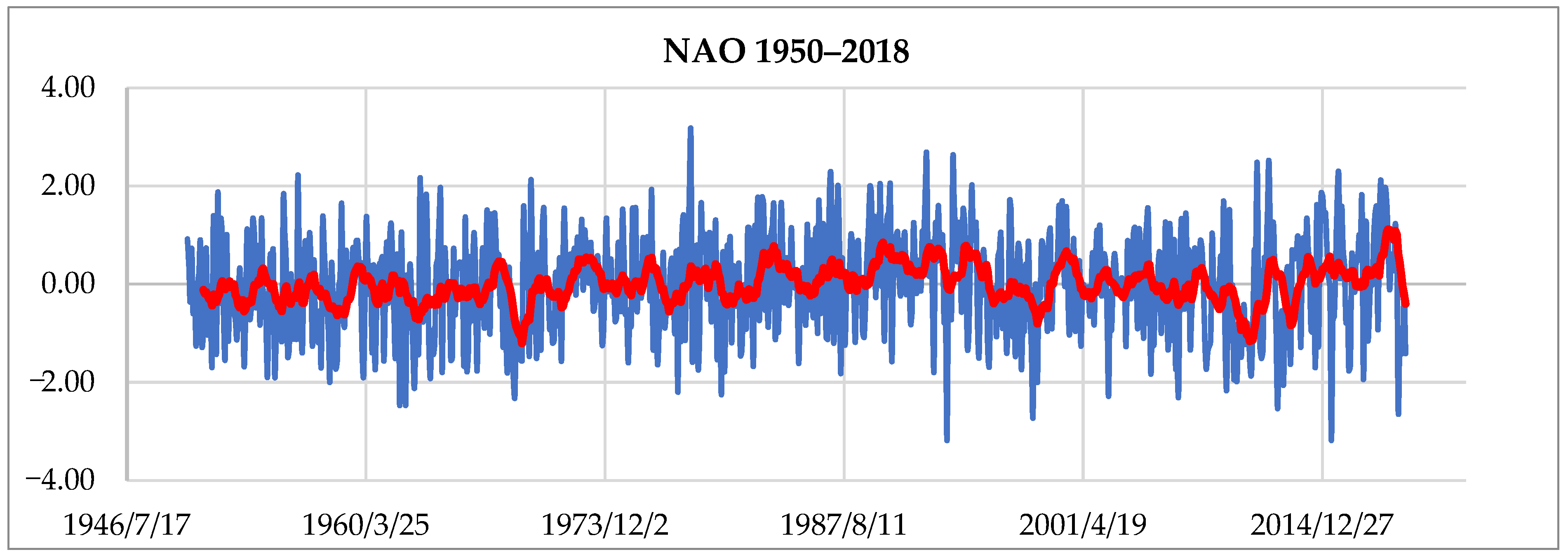
- NOAA data (National Oceanographic and Atmospheric Centre, Silver Spring, Maryland, USA) from NCEP reanalysis (1948–2018) [94];
- Global climate projections (2041–2070) [77].
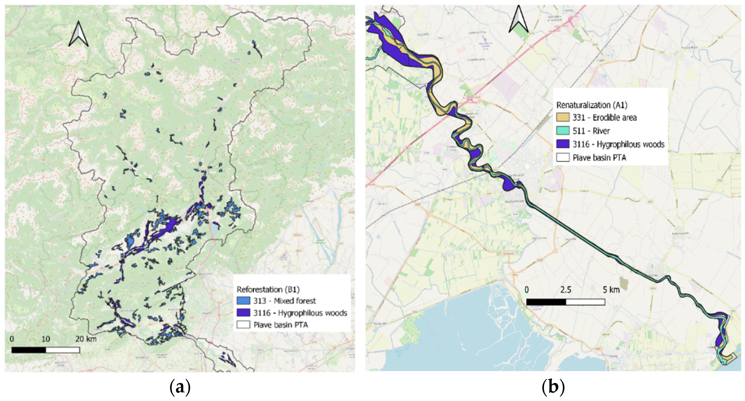
2.5. NBS Scenarios
2.6. Cost Analysis of N and P
3. Results
3.1. Climate Change
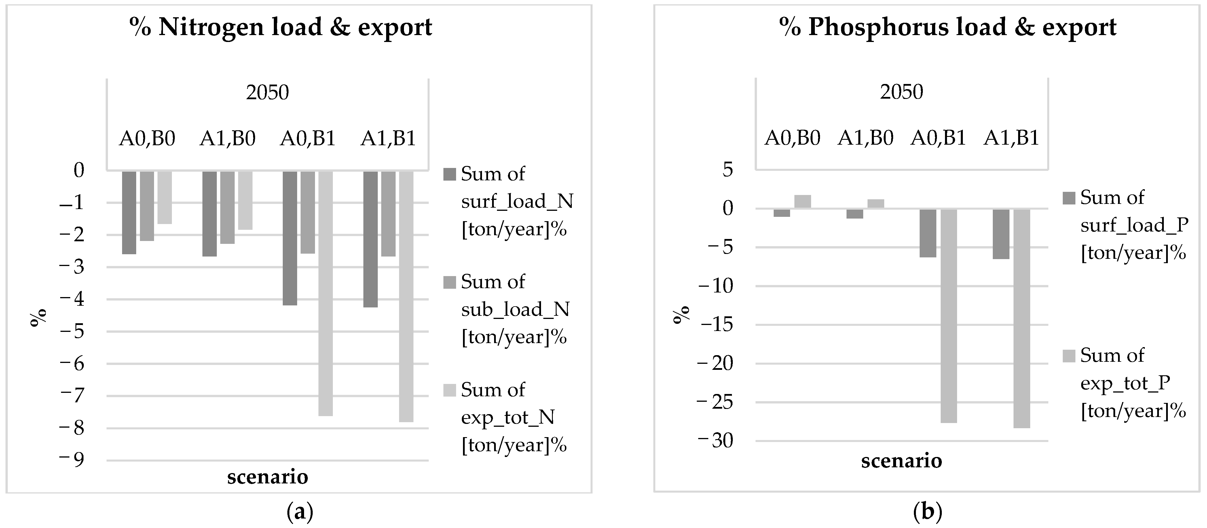
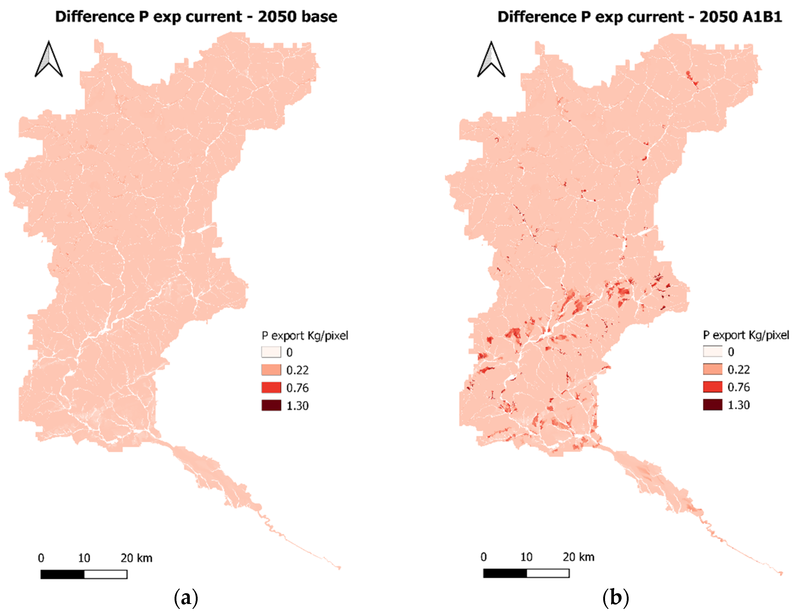
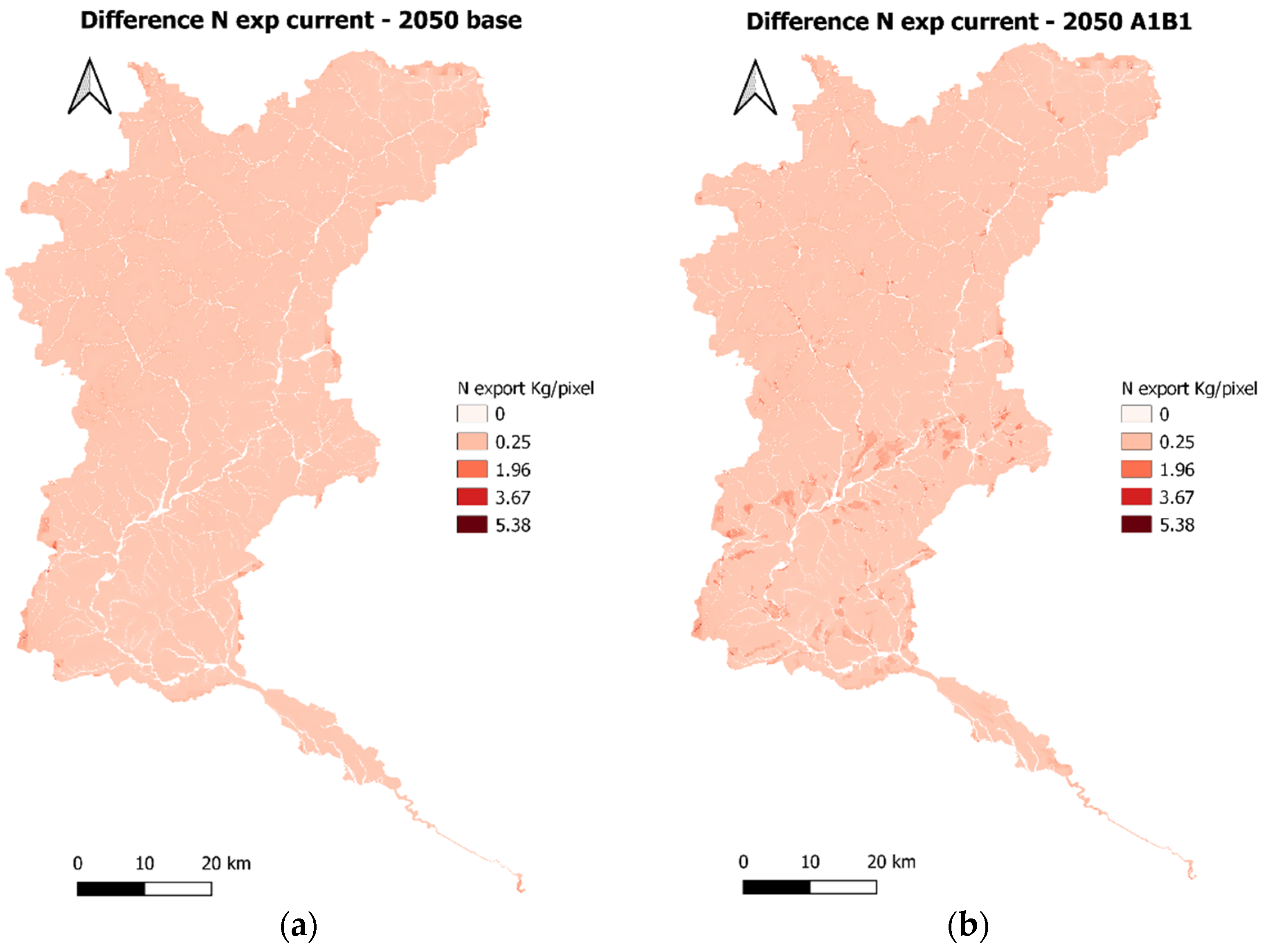
3.2. Nutrient Export
4. Discussion
4.1. Nutrient Dynamics and Distribution
4.2. ESs Evaluation of NBS
5. Conclusions
Supplementary Materials
Author Contributions
Funding
Institutional Review Board Statement
Informed Consent Statement
Data Availability Statement
Acknowledgments
Conflicts of Interest
References
- Millenium Ecosystem Assessment. Ecosystems and Human Well-Being: General Synthesis; Island Press: Washington, DC, USA, 2005. [Google Scholar]
- Costanza, R.; D‘Arge, R.; De Groot, R.; Farber, S.; Grasso, M.; Hannon, B.; Limburg, K.; Naeem, S.; O’Neill, R.V.; Paruelo, J.M.; et al. The value of the world’s ecosystem services and natural capital. Nature 1997, 387, 253–260. [Google Scholar] [CrossRef]
- Foley, J.A.; DeFries, R.; Asner, G.; Barford, C.; Bonan, G.; Carpenter, S.R.; Chapin, F.S.; Coe, M.; Daily, G.C.; Gibbs, H.K.; et al. Global consequences of land use. Science 2005, 309, 570–574. [Google Scholar] [CrossRef] [PubMed] [Green Version]
- Carpenter, S.R.; Mooney, H.A.; Agard, J.; Capistrano, D.; DeFries, R.S.; Díaz, S.; Dietz, T.; Duraiappah, A.K.; Oteng-Yeboah, A.; Pereira, H.M. Science for managing ecosystem services: Beyond the Millennium ecosystem assessment. Proc. Natl. Acad. Sci. USA 2009, 106, 1305–1312. [Google Scholar] [CrossRef] [PubMed] [Green Version]
- Sharps, K.; Masante, D.; Thomas, A.; Jackson, B.; Redhead, J.; May, L.; Prosser, H.; Cosby, B.; Emmett, B.; Jones, L. Comparing strengths and weaknesses of three ecosystem services modelling tools in a diverse UK river catchment. Sci. Total Environ. 2017, 584–585, 118–130. [Google Scholar] [CrossRef] [PubMed] [Green Version]
- Silvertown, J. A new dawn for citizen science. Trends Ecol. Evol. 2009, 24, 467–471. [Google Scholar] [CrossRef] [PubMed]
- Bonter, D.; Cooper, C.B. Data validation in citizen science: A case study from Project FeederWatch. Front. Ecol. Environ. 2012, 10, 305–307. [Google Scholar] [CrossRef]
- Bonney, R.; Shirk, J.L.; Phillips, T.B.; Wiggins, A.; Ballard, H.L.; Miller-Rushing, A.J.; Parrish, J.K. Next steps for citizen science. Science 2014, 343, 1436–1437. [Google Scholar] [CrossRef]
- Dickinson, J.L.; Shirk, J.; Bonter, D.; Bonney, R.; Crain, R.; Martin, J.; Phillips, T.B.; Purcell, K. The current state of citizen science as a tool for ecological research and public engagement. Front. Ecol. Environ. 2012, 10, 291–297. [Google Scholar] [CrossRef] [Green Version]
- Buytaert, W.; Zulkafli, Z.; Grainger, S.; Acosta, L.; Alemie, T.C.; Bastiaensen, J.; De Bièvre, B.; Bhusal, J.; Clark, J.; Dewulf, A.; et al. Citizen science in hydrology and water resources: Opportunities for knowledge generation, ecosystem service management, and sustainable development. Front. Earth Sci. 2014, 2. [Google Scholar] [CrossRef] [Green Version]
- Fritz, S.; See, L.; Carlson, T.; Haklay, M.; Oliver, J.L.; Fraisl, D.; Mondardini, R.; Brocklehurst, M.; Shanley, L.A.; Schade, S.; et al. Citizen science and the United Nations sustainable development goals. Nat. Sustain. 2019, 2, 922–930. [Google Scholar] [CrossRef]
- Njue, N.; Kroese, J.S.; Gräf, J.; Jacobs, S.; Weeser, B.; Breuer, L.; Rufino, M. Citizen science in hydrological monitoring and ecosystem services management: State of the art and future prospects. Sci. Total Environ. 2019, 693, 133531. [Google Scholar] [CrossRef]
- Pandeya, B.; Buytaert, W.; Potter, C. Designing citizen science for water and ecosystem services management in data-poor regions: Challenges and opportunities. Curr. Res. Environ. Sustain. 2021, 3, 100059. [Google Scholar] [CrossRef]
- Miller-Rushing, A.; Primack, R.B.; Bonney, R. The history of public participation in ecological research. Front. Ecol. Environ. 2012, 10, 285–290. [Google Scholar] [CrossRef]
- Theobald, E.; Ettinger, A.; Burgess, H.; DeBey, L.; Schmidt, N.; Froehlich, H.; Wagner, C.; HilleRisLambers, J.; Tewksbury, J.; Harsch, M.; et al. Global change and local solutions: Tapping the unrealized potential of citizen science for biodiversity research. Biol. Conserv. 2014, 181, 236–244. [Google Scholar] [CrossRef] [Green Version]
- McKinley, D.C.; Miller-Rushing, A.J.; Ballard, H.L.; Bonney, R.; Brown, H.; Cook-Patton, S.C.; Evans, D.M.; French, R.A.; Parrish, J.K.; Phillips, T.B.; et al. Citizen science can improve conservation science, natural resource management, and environmental protection. Biol. Conserv. 2017, 208, 15–28. [Google Scholar] [CrossRef] [Green Version]
- Kullenberg, C.; Kasperowski, D. What is citizen science? A Scientometric Meta-Analysis. PLoS ONE 2016, 11, e0147152. [Google Scholar] [CrossRef] [Green Version]
- Schröter, M.; Kraemer, R.; Mantel, M.; Kabisch, N.; Hecker, S.; Richter, A.; Neumeier, V.; Bonn, A. Citizen science for assessing ecosystem services: Status, challenges and opportunities. Ecosyst. Serv. 2017, 28, 80–94. [Google Scholar] [CrossRef]
- Raudsepp-Hearne, C.; Peterson, G.; Bennett, E.M. Ecosystem service bundles for analyzing tradeoffs in diverse landscapes. Proc. Natl. Acad. Sci. USA 2010, 107, 5242–5247. [Google Scholar] [CrossRef] [PubMed] [Green Version]
- Schröter, M.; van der Zanden, E.M.; van Oudenhoven, A.P.E.; Remme, R.P.; Serna-Chavez, H.M.; de Groot, R.S.; Opdam, P. Ecosystem services as a contested concept: A synthesis of critique and counter-arguments. Conserv. Lett. 2014, 7, 514–523. [Google Scholar] [CrossRef] [Green Version]
- Kabisch, N.; Qureshi, S.; Haase, D. Human-environment interactions in urban green spaces—A systematic review of contemporary issues and prospects for future research. Environ. Impact Assess. Rev. 2015, 50, 25–34. [Google Scholar] [CrossRef]
- Bishop, I.J.; Warner, S.; Van Noordwijk, T.C.G.E.; Nyoni, F.C.; Loiselle, S. Citizen science monitoring for sustainable development goal indicator 6.3.2 in England and Zambia. Sustainability 2020, 12, 10271. [Google Scholar] [CrossRef]
- Fraisl, D.; Campbell, J.; See, L.; Wehn, U.; Wardlaw, J.; Gold, M.; Moorthy, I.; Arias, R.; Piera, J.; Oliver, J.L.; et al. Mapping citizen science contributions to the UN sustainable development goals. Sustain. Sci. 2020, 15, 1735–1751. [Google Scholar] [CrossRef]
- Keeler, B.L.; Polasky, S.; Brauman, K.; Johnson, K.A.; Finlay, J.; O’Neill, A.; Kovacs, K.; Dalzell, B. Linking water quality and well-being for improved assessment and valuation of ecosystem services. Proc. Natl. Acad. Sci. USA 2012, 109, 18619–18624. [Google Scholar] [CrossRef] [PubMed] [Green Version]
- Pereda, O.; von Schiller, D.; García-Baquero, G.; Mor, J.-R.; Acuña, V.; Sabater, S.; Elosegi, A. Combined effects of urban pollution and hydrological stress on ecosystem functions of Mediterranean streams. Sci. Total Environ. 2020, 753, 141971. [Google Scholar] [CrossRef]
- Vigerstol, K.L.; Aukema, J.E. A comparison of tools for modeling freshwater ecosystem services. J. Environ. Manag. 2011, 92, 2403–2409. [Google Scholar] [CrossRef]
- Sharp, R.; Tallis, H.T.; Ricketts, T.; Guerry, A.D.; Wood, S.A.; Chaplin-Kramer, R.; Nelson, E.; Ennaanay, D.; Wolny, S.; Olwero, N.; et al. InVEST User Guide—InVEST + VERSION + Documentation. Available online: https://invest-userguide.readthedocs.io/en/3.5.0/ (accessed on 3 August 2021).
- Garnier, J.; Billen, G.; Lassaletta, L.; Vigiak, O.; Nikolaidis, N.P.; Grizzetti, B. Hydromorphology of coastal zone and structure of watershed agro-food system are main determinants of coastal eutrophication. Environ. Res. Lett. 2021, 16, 023005. [Google Scholar] [CrossRef]
- Lancelot, C.; Thieu, V.; Polard, A.; Garnier, J.; Billen, G.; Hecq, W.; Gypens, N. Cost assessment and ecological effectiveness of nutrient reduction options for mitigating Phaeocystis colony blooms in the Southern North Sea: An integrated modeling approach. Sci. Total Environ. 2011, 409, 2179–2191. [Google Scholar] [CrossRef] [PubMed]
- Billen, G.; Garnier, J. The Phison River plume: Coastal eutrophication in response to changes in land use and water management in the watershed. Aquat. Microb. Ecol. 1997, 13, 3–17. [Google Scholar] [CrossRef]
- McCrackin, M.L.; Muller-Karulis, B.; Gustafsson, B.G.; Howarth, R.W.; Humborg, C.; Svanbäck, A.; Swaney, D.P. A century of legacy phosphorus dynamics in a large drainage basin. Glob. Biogeochem. Cycles 2018, 32, 1107–1122. [Google Scholar] [CrossRef]
- Turner, R.E.; Rabalais, N.N. Coastal eutrophication near the Mississippi river delta. Nature 1994, 368, 619–621. [Google Scholar] [CrossRef]
- Turner, R.E.; Rabalais, N.N.; Justic’, D.; Dortch, Q. Future aquatic nutrient limitations. Mar. Pollut. Bull. 2003, 46, 1032–1034. [Google Scholar] [CrossRef]
- Cui, L.; Lu, X.; Dong, Y.; Cen, J.; Cao, R.; Pan, L.; Lu, S.; Ou, L. Relationship between phytoplankton community succession and environmental parameters in Qinhuangdao coastal areas, China: A region with recurrent brown tide outbreaks. Ecotoxicol. Environ. Saf. 2018, 159, 85–93. [Google Scholar] [CrossRef]
- Liu, X.; Beusen, A.; Van Beek, L.P.; Mogollón, J.M.; Ran, X.; Bouwman, L. Exploring spatiotemporal changes of the Yangtze River (Changjiang) nitrogen and phosphorus sources, retention and export to the East China Sea and Yellow Sea. Water Res. 2018, 142, 246–255. [Google Scholar] [CrossRef] [PubMed]
- Directive 2000/60/EC of the European Parliament and of the Council of 23 October 2000. Establishing a framework for Community action in the field of water policy. Off. J. Eur. Parliam. 2000, L327, 1–82.
- European Council. Establishing common rules for direct support schemes for farmers under the common agricultural policy and establishing certain support schemes for farmers, amending Regulations (EC) No 1290/2005, (EC) No 247/2006, (EC) No 378/2007 and repealing Regulation. Eur. Rural Dev. Policy 2009, 73, 16–99. [Google Scholar]
- Grizzetti, B.; Bouraoui, F.; Aloe, A. Changes of nitrogen and phosphorus loads to European seas. Glob. Chang. Biol. 2011, 18, 769–782. [Google Scholar] [CrossRef]
- Romero, E.; Garnier, J.; Lassaletta, L.; Billen, G.; Le Gendre, R.; Riou, P.; Cugier, P. Large-scale patterns of river inputs in southwestern Europe: Seasonal and interannual variations and potential eutrophication effects at the coastal zone. Biodegradation 2012, 113, 481–505. [Google Scholar] [CrossRef] [Green Version]
- Pistocchi, A.; Dorati, C.; Grizzetti, B.; Udias, A.; Vigiak, O.; Zanni, M. Water Quality in Europe: Effects of the Urban Wastewater Treatment Directive. A Retrospective and Scenario Analysis of Dir. 91/271/EEC; EUR 30003 EN; Publications Office of the European Union: Luxembourg, 2019; pp. 1–112. [Google Scholar] [CrossRef]
- Rabalais, N.N.; Turner, R.E.; Scavia, D. Beyond Science into Policy: Gulf of Mexico Hypoxia and the Mississippi River. BioScience 2002, 52, 129–142. [Google Scholar] [CrossRef] [Green Version]
- Turner, B.L.; Lambin, E.F.; Reenberg, A. The emergence of land change science for global environmental change and sustainability. Proc. Natl. Acad. Sci. USA 2007, 104, 20666–20671. [Google Scholar] [CrossRef] [Green Version]
- Shu, L.; Finlayson, B. Flood management on the lower Yellow River: Hydrological and geomorphological perspectives. Sediment. Geol. 1993, 85, 285–296. [Google Scholar] [CrossRef]
- Wang, H.; Yang, Z.; Saito, Y.; Liu, P.; Sun, X. Interannual and seasonal variation of the Huanghe (Yellow River) water discharge over the past 50 years: Connections to impacts from ENSO events and dams. Glob. Planet. Chang. 2006, 50, 212–225. [Google Scholar] [CrossRef]
- Ma, T.; Zhao, N.; Ni, Y.; Yi, J.; Wilson, J.P.; He, L.; Du, Y.; Pei, T.; Zhou, C.; Song, C.; et al. China’s improving inland surface water quality since 2003. Sci. Adv. 2020, 6, eaau3798. [Google Scholar] [CrossRef] [PubMed] [Green Version]
- Garnier, J.; Marescaux, A.; Guillon, S.; Vilmin, L.; Rocher, V.; Billen, G.; Thieu, V.; Silvestre, M.; Passy, P.; Raimonet, M.; et al. Ecological functioning of the Seine River: From Long-term modelling approaches to high-frequency data analysis. In Handbook of Environmental Chemistry; Science and Business Media Deutschland: Berlin, Germany, 2020; pp. 189–216. [Google Scholar] [CrossRef]
- Torrecilla, N.J.; Galve, J.P.; Zaera, L.G.; Retamar, J.F.; Álvarez, A.N. Nutrient sources and dynamics in a mediterranean fluvial regime (Ebro River, NE Spain) and their implications for water management. J. Hydrol. 2005, 304, 166–182. [Google Scholar] [CrossRef]
- Minaudo, C.; Meybeck, M.; Moatar, F.; Gassama, N.; Curie, F. Eutrophication mitigation in rivers: 30 years of trends in spatial and seasonal patterns of biogeochemistry of the Loire River (1980–2012). Biogeosciences 2015, 12, 2549–2563. [Google Scholar] [CrossRef] [Green Version]
- Passy, P.; Le Gendre, R.; Garnier, J.; Cugier, P.; Callens, J.; Paris, F.; Billen, G.; Riou, P.; Romero, E. Eutrophication modelling chain for improved management strategies to prevent algal blooms in the Bay of Seine. Mar. Ecol. Prog. Ser. 2016, 543, 107–125. [Google Scholar] [CrossRef] [Green Version]
- Desmit, X.; Thieu, V.; Billen, G.; Campuzano, F.; Dulière, V.; Garnier, J.; Lassaletta, L.; Ménesguen, A.; Neves, R.; Pinto, L.; et al. Reducing marine eutrophication may require a paradigmatic change. Sci. Total Environ. 2018, 635, 1444–1466. [Google Scholar] [CrossRef]
- Garnier, J.; Riou, P.; Le Gendre, R.; Ramarson, A.; Billen, G.; Cugier, P.; Schapira, M.; Théry, S.; Thieu, V.; Ménesguen, A. Managing the agri-food system of watersheds to combat coastal eutrophication: A land-to-sea modelling approach to the French coastal English Channel. Geosciences 2019, 9, 441. [Google Scholar] [CrossRef] [Green Version]
- Gumiero, B.; Cornelio, P.; Boz, B. Nitrogen removal by an irrigated wooded buffer area. Water Pract. Technol. 2011, 6, 1–2. [Google Scholar] [CrossRef]
- Kuglerová, L.; Ågren, A.; Jansson, R.; Laudon, H. Towards optimizing riparian buffer zones: Ecological and biogeochemical implications for forest management. For. Ecol. Manag. 2014, 334, 74–84. [Google Scholar] [CrossRef]
- Ou, Y.; Wang, X.; Wang, L.; Rousseau, A.N. Landscape influences on water quality in riparian buffer zone of drinking water source area, Northern China. Environ. Earth Sci. 2016, 75, 1–13. [Google Scholar] [CrossRef]
- De Mello, K.; Randhir, T.O.; Valente, R.A.; Vettorazzi, C.A. Riparian restoration for protecting water quality in tropical agricultural watersheds. Ecol. Eng. 2017, 108, 514–524. [Google Scholar] [CrossRef]
- Gumiero, B.; Boz, B. How to stop nitrogen leaking from a Cross compliant buffer strip? Ecol. Eng. 2017, 103, 446–454. [Google Scholar] [CrossRef]
- Sabater, S.; Butturini, A.; Clement, J.-C.; Burt, T.; Dowrick, D.; Hefting, M.; Maître, V.; Pinay, G.; Postolache, C.; Rzepecki, M.; et al. Nitrogen removal by riparian buffers along a european climatic gradient: Patterns and factors of variation. Ecosystems 2003, 6, 20–30. [Google Scholar] [CrossRef]
- Sweeney, B.W.; Bott, T.L.; Jackson, J.K.; Kaplan, L.A.; Newbold, J.D.; Standley, L.J.; Hession, W.C.; Horwitz, R.J. Riparian deforestation, stream narrowing, and loss of stream ecosystem services. Proc. Natl. Acad. Sci. USA 2004, 101, 14132–14137. [Google Scholar] [CrossRef] [PubMed] [Green Version]
- Schilling, K.E.; Jacobson, P. Effectiveness of natural riparian buffers to reduce subsurface nutrient losses to incised streams. Catena 2014, 114, 140–148. [Google Scholar] [CrossRef]
- Loiselle, S.; Cunha, D.G.F.; Shupe, S.; Valiente, E.; Rocha, L.; Heasley, E.; Belmont, P.P.; Baruch, A. Micro and macroscale drivers of nutrient concentrations in urban streams in South, Central and North America. PLoS ONE 2016, 11, e0162684. [Google Scholar] [CrossRef] [Green Version]
- Tanaka, M.O.; de Souza, A.L.T.; Moschini, L.E.; de Oliveira, A.K. Influence of watershed land use and riparian characteristics on biological indicators of stream water quality in southeastern Brazil. Agric. Ecosyst. Environ. 2016, 216, 333–339. [Google Scholar] [CrossRef]
- Saalfeld, D.T.; Reutebuch, E.M.; Dickey, R.J.; Seesock, W.C.; Webber, C.; Bayne, D.R. Effects of landscape characteristics on water quality and fish assemblages in the Tallapoosa River Basin, Alabama. Southeast. Nat. 2012, 11, 239–252. [Google Scholar] [CrossRef]
- Ding, S.; Zhang, Y.; Liu, B.; Kong, W.; Meng, W. Effects of riparian land use on water quality and fish communities in the headwater stream of the Taizi River in China. Front. Environ. Sci. Eng. 2013, 7, 699–708. [Google Scholar] [CrossRef]
- Yang, H.; Wang, G.; Wang, L.; Zheng, B. Impact of land use changes on water quality in headwaters of the Three Gorges Reservoir. Environ. Sci. Pollut. Res. 2015, 23, 11448–11460. [Google Scholar] [CrossRef]
- Zhang, X.; Liu, X.; Zhang, M.; Dahlgren, R.A.; Eitzel, M. A Review of vegetated buffers and a meta-analysis of their mitigation efficacy in reducing nonpoint source pollution. J. Environ. Qual. 2010, 39, 76–84. [Google Scholar] [CrossRef]
- Yang, W.; Liu, Y.; Ou, C.; Gabor, S. Examining water quality effects of riparian wetland loss and restoration scenarios in a southern ontario watershed. J. Environ. Manag. 2016, 174, 26–34. [Google Scholar] [CrossRef] [PubMed]
- Glibert, P.M.; Allen, J.I.; Artioli, Y.; Beusen, A.; Bouwman, L.; Harle, J.; Holmes, R.; Holt, J. Vulnerability of coastal ecosystems to changes in harmful algal bloom distribution in response to climate change: Projections based on model analysis. Glob. Chang. Biol. 2014, 20, 3845–3858. [Google Scholar] [CrossRef]
- Wåhlström, I.; Höglund, A.; Almroth-Rosell, E.; MacKenzie, B.R.; Gröger, M.; Eilola, K.; Plikshs, M.; Andersson, H.C. Combined climate change and nutrient load impacts on future habitats and eutrophication indicators in a eutrophic coastal sea. Limnol. Oceanogr. 2020, 65, 2170–2187. [Google Scholar] [CrossRef]
- Whitehead, P.G.; Wilby, R.L.; Battarbee, R.W.; Kernan, M.; Wade, A. A review of the potential impacts of climate change on surface water quality. Hydrol. Sci. J. 2009, 54, 101–123. [Google Scholar] [CrossRef]
- Garnier, J.; Ramarson, A.; Billen, G.; Théry, S.; Thiéry, D.; Thieu, V.; Minaudo, C.; Moatar, F. Nutrient inputs and hydrology together determine biogeochemical status of the Loire River (France): Current situation and possible future scenarios. Sci. Total Environ. 2018, 637–638, 609–624. [Google Scholar] [CrossRef] [PubMed] [Green Version]
- Raimonet, M.; Thieu, V.; Silvestre, M.; Oudin, L.; Rabouille, C.; Vautard, R.; Garnier, J. Landward perspective of coastal eutrophication potential under future climate change: The Seine River case. Front. Mar. Sci. 2018, 5. [Google Scholar] [CrossRef] [Green Version]
- Duan, H.; Ma, R.; Zhang, Y.; Loiselle, S.A. Are algal blooms occurring later in Lake Taihu? Climate local effects outcompete mitigation prevention. J. Plankton Res. 2014, 36, 866–871. [Google Scholar] [CrossRef] [Green Version]
- Botter, G.; Basso, S.; Porporato, A.; Rodriguez-Iturbe, I.; Rinaldo, A. Natural streamflow regime alterations: Damming of the Piave river basin. Water Resour. Res. 2010, 46. [Google Scholar] [CrossRef]
- Romero, E.; Le Gendre, R.; Garnier, J.; Billen, G.; Fisson, C.; Silvestre, M.; Riou, P. Long-term water quality in the lower Seine: Lessons learned over 4 decades of monitoring. Environ. Sci. Policy 2016, 58, 141–154. [Google Scholar] [CrossRef] [Green Version]
- ISPRA. DEM 20m—Italy. Available online: http://www.sinanet.isprambiente.it/it/sia-ispra/download-mais/dem20/view (accessed on 3 August 2021).
- ISPRA. Corine Land Cover 2018 IV livello|Uso, copertura e consumo di suolo. Available online: http://groupware.sinanet.isprambiente.it/uso-copertura-e-consumo-di-suolo/library/copertura-del-suolo/corine-land-cover/corine-land-cover-2018-iv-livello (accessed on 3 August 2021).
- Dezsi, Ş.; Mîndrescu, M.; Petrea, D.; Rai, P.K.; Hamann, A.; Nistor, M.-M. High-resolution projections of evapotranspiration and water availability for Europe under climate change. Int. J. Clim. 2018, 38, 3832–3841. [Google Scholar] [CrossRef]
- ARPAV. Bacini Idrografici del Piano di Tutela delle Acque—Geomap ARPAV. Available online: http://geomap.arpa.veneto.it/layers/geonode%3Abacinipta (accessed on 3 August 2021).
- ARPAV. Corpi idrici fluviali (Progetti di Piano, 2020)—Geomap ARPAV. Available online: http://geomap.arpa.veneto.it/layers/geonode%3Acorpi_idrici_fluviali (accessed on 3 August 2021).
- Borselli, L.; Cassi, P.; Torri, D. Prolegomena to sediment and flow connectivity in the landscape: A GIS and field numerical assessment. Catena 2008, 75, 268–277. [Google Scholar] [CrossRef]
- ARPAV. Carichi di Azoto Agricolo, da Allevamento e da Fertilizzanti—Geomap ARPAV. Available online: http://geomap.arpa.veneto.it/layers/geonode%3Acarichi_azotoagricolo (accessed on 3 August 2021).
- ARPAV. Carta del Rischio di Percolazione Dell’azoto-Geomap ARPAV. Available online: http://geomap.arpa.veneto.it/maps/270 (accessed on 3 August 2021).
- ARPAV; Giandon, P.; Carta Della Capacità Protettiva E Del Rischio Di Percolazione Dell’azoto Dei Suoli Della Pianura Veneta. Report 2016. Available online: https://www.arpa.veneto.it/temi-ambientali/suolo/file-e-allegati/documenti/minacce-di-degradazione/Cap_prot_relazione_2016.pdf (accessed on 3 August 2021).
- ARPAV. Capacità Protettiva dei Suoli—Geomap ARPAV. Available online: http://geomap.arpa.veneto.it/layers/geonode%3Acaprotsuoli (accessed on 3 August 2021).
- ARPAV. Acque sotterranee-Concentrazione di Nitrati. Available online: https://www.arpa.veneto.it/dati-ambientali/open-data/idrosfera/acque-sotterranee/acque-sotterranee-concentrazione-di-nitrati (accessed on 3 August 2021).
- Pärn, J.; Pinay, G.; Mander, Ü. Indicators of nutrients transport from agricultural catchments under temperate climate: A review. Ecol. Indic. 2012, 22, 4–15. [Google Scholar] [CrossRef]
- Mayer, P.M.; Reynolds, S.K.; McCutchen, M.D.; Canfield, T.J. Meta-analysis of nitrogen removal in riparian buffers. J. Environ. Qual. 2007, 36, 1172–1180. [Google Scholar] [CrossRef]
- FreshWater Watch Methods Manual. Available online: https://freshwaterwatch.thewaterhub.org/sites/default/files/fww-methods-manual.pdf (accessed on 3 August 2021).
- Scott, A.B.; Frost, P.C. Monitoring water quality in Toronto’s urban stormwater ponds: Assessing participation rates and data quality of water sampling by citizen scientists in the FreshWater Watch. Sci. Total Environ. 2017, 592, 738–744. [Google Scholar] [CrossRef] [PubMed]
- Thornhill, I.; Chautard, A.; Loiselle, S. Monitoring biological and chemical trends in temperate still waters using citizen science. Water 2018, 10, 839. [Google Scholar] [CrossRef] [Green Version]
- Strickland, J.D.H.; Parsons, T.R. A practical handbook of seawater analysis. Bull. Fish. Res. Board Can. 1972, 167, 405. [Google Scholar]
- Law, A.T.; Adeloju, S.B. Progress and recent advances in phosphate sensors: A review. Talanta 2013, 114, 191–203. [Google Scholar] [CrossRef]
- ARPAV. Meteo & Clim—from 1994 to 2020. Available online: https://www.arpa.veneto.it/dati-ambientali/open-data/clima (accessed on 3 August 2021).
- NOAA. NCEP/NCAR Reanalysis 1: NOAA Physical Sciences Laboratory. Available online: https://psl.noaa.gov/data/gridded/data.ncep.reanalysis.html (accessed on 3 August 2021).
- Wanner, H.; Brönnimann, S.; Casty, C.; Gyalistras, D.; Luterbacher, J.; Schmutz, C.; Stephenson, D.B.; Xoplaki, E. North Atlantic Oscillation–Concepts and Studies. Surv. Geophys. 2001, 22, 321–381. [Google Scholar] [CrossRef]
- Hurrell, J.W.; Kushnir, Y.; Ottersen, G.; Visbeck, M. An overview of the North Atlantic Oscillation. Geophys. Monogr. Ser. 2003, 134, 1–35. [Google Scholar] [CrossRef] [Green Version]
- Daly, C.; Halbleib, M.; Smith, J.I.; Gibson, W.P.; Doggett, M.K.; Taylor, G.H.; Curtis, J.; Pasteris, P.P. Physiographically sensitive mapping of climatological temperature and precipitation across the conterminous United States. Int. J. Clim. 2008, 28, 2031–2064. [Google Scholar] [CrossRef]
- Copernicus. Coperenicus (clc2018). Available online: https://land.copernicus.eu/pan-european/corine-land-cover/clc2018 (accessed on 13 April 2019).
- Picco, L.; Comiti, F.; Mao, L.; Tonon, A.; Lenzi, M. Medium and short term riparian vegetation, island and channel evolution in response to human pressure in a regulated gravel bed river (Piave River, Italy). Catena 2017, 149, 760–769. [Google Scholar] [CrossRef]
- Consorzio di Bonifica Acque Risorgive. Interventi Riqualificazione. Available online: https://www.acquerisorgive.it/ambiente/documentazione/interventi-riqualificazione/ (accessed on 3 August 2021).
- Jiang, F.; Beck, M.B.; Cummings, R.G.; Rowles, K.; Russell, D. Estimation of Costs Of phosphorus removal in wastewater treatment facilities: Construction de novo. Water Policy Work. Pap. 2004, 2004, 28. Available online: http://citeseerx.ist.psu.edu/viewdoc/download?doi=10.1.1.553.4588&rep=rep1&type=pdf (accessed on 3 August 2021).
- Strokal, M.; Kroeze, C.; Wang, M.; Bai, Z.; Ma, L. The MARINA model (Model to Assess River Inputs of Nutrients to seAs): Model description and results for China. Sci. Total Environ. 2016, 562, 869–888. [Google Scholar] [CrossRef] [Green Version]
- Bashar, R.; Gungor, K.; Karthikeyan, K.; Barak, P. Cost effectiveness of phosphorus removal processes in municipal wastewater treatment. Chemosphere 2018, 197, 280–290. [Google Scholar] [CrossRef]
- Gratziou, M.; Chrisochoidou, P. Cost analysis of wastewater nitrogen removal in Greece. Fresenius Environ. Bull. 2013, 22, 2117–2123. [Google Scholar]
- Bladé, I.; Liebmann, B.; Fortuny, D.; van Oldenborgh, G.J. Observed and simulated impacts of the summer NAO in Europe: Implications for projected drying in the Mediterranean region. Clim. Dyn. 2011, 39, 709–727. [Google Scholar] [CrossRef]
- Meehl, G.A.; Covey, C.; Delworth, T.; Latif, M.; McAvaney, B.; Mitchell, F.B.; Stouffer, R.J.; Taylor, K.E. The WCRP CMIP3 multimodel dataset: A new era in climate change research. Bull. Am. Meteorol. Soc. 2007, 88, 1383–1394. [Google Scholar] [CrossRef] [Green Version]
- Baruffi, F.; Cisotto, A.; Cimolino, A.; Ferri, M.; Monego, M.; Norbiato, D.; Cappelletto, M.; Bisaglia, M.; Pretner, A.; Galli, A.; et al. Climate change impact assessment on Veneto and Friuli plain groundwater. Part I: An integrated modeling approach for hazard scenario construction. Sci. Total Environ. 2012, 440, 154–166. [Google Scholar] [CrossRef] [PubMed]
- Stocker, T.F.; Qin, D.; Plattner, G.K.; Tignor, M.; Allen, S.K.; Boschung, J.; Nauels, A.; Xia, Y.; Bex, V.; Midgley, P.M. Ipcc, 2013: Climate change 2013: The physical science basis. In Contribution of Working Group I to the Fifth Assessment Report of the Intergovernmental Panel on Climate Change; Cambridge University Press: Cambridge, UK, 2013; Volume 1535, Available online: https://www.eea.europa.eu/data-and-maps/indicators/global-and-european-temperature-9/ipcc-2013-summary-for-policymakers-2013 (accessed on 3 August 2021).
- ARPAV. La rete idrometrica e le portate. Available online: https://www.arpa.veneto.it/temi-ambientali/idrologia/file-e-allegati/rapporti-e-documenti/idrologia-regionale/idrologia-regionale-la-rete-idrometrica (accessed on 3 August 2021).
- Redhead, J.W.; May, L.; Oliver, T.H.; Hamel, P.; Sharp, R.; Bullock, J.M. National scale evaluation of the InVEST nutrient retention model in the United Kingdom. Sci. Total Environ. 2018, 610, 666–677. [Google Scholar] [CrossRef]
- Seddon, N.; Chausson, A.; Berry, P.; Girardin, C.A.J.; Smith, A.; Turner, B. Understanding the value and limits of nature-based solutions to climate change and other global challenges. Philos. Trans. R. Soc. B Biol. Sci. 2020, 375, 20190120. [Google Scholar] [CrossRef] [PubMed] [Green Version]
- Lasanta, T.; Arnáez, J.; Pascual, N.; Ruiz, P.; Errea, M.; Lana-Renault, N. Space–time process and drivers of land abandonment in Europe. Catena 2017, 149, 810–823. [Google Scholar] [CrossRef]
- Malavasi, M.; Carranza, M.L.; Moravec, D.; Cutini, M. Reforestation dynamics after land abandonment: A trajectory analysis in Mediterranean mountain landscapes. Reg. Environ. Chang. 2018, 18, 2459–2469. [Google Scholar] [CrossRef]
- Rocchini, D.; Perry, G.L.; Salerno, M.; Maccherini, S.; Chiarucci, A. Landscape change and the dynamics of open formations in a natural reserve. Landsc. Urban Plan. 2006, 77, 167–177. [Google Scholar] [CrossRef]
- Wade, A.J.; Butterfield, D.; Whitehead, P. Towards an improved understanding of the nitrate dynamics in lowland, permeable river-systems: Applications of INCA-N. J. Hydrol. 2006, 330, 185–203. [Google Scholar] [CrossRef]
- Tasser, E.; Mader, M.; Tappeiner, U. Effects of land use in alpine grasslands on the probability of landslides. Basic Appl. Ecol. 2003, 4, 271–280. [Google Scholar] [CrossRef]
- Seeber, J.; Seeber, G. Effects of land-use changes on humus forms on alpine pastureland (Central Alps, Tyrol). Geoderma 2005, 124, 215–222. [Google Scholar] [CrossRef]
- Fox, G.A.; Purvis, R.A.; Penn, C.J. Streambanks: A net source of sediment and phosphorus to streams and rivers. J. Environ. Manag. 2016, 181, 602–614. [Google Scholar] [CrossRef] [Green Version]
- Cozzi, S.; Ibáñez, C.; Lazar, L.; Raimbault, P.; Giani, M. Flow regime and nutrient-loading trends from the largest South European Watersheds: Implications for the productivity of Mediterranean and Black Sea’s coastal areas. Water 2018, 11, 1. [Google Scholar] [CrossRef] [Green Version]
- Jabłońska, E.; Wiśniewska, M.; Marcinkowski, P.; Grygoruk, M.; Walton, C.R.; Zak, D.; Hoffmann, C.C.; Larsen, S.E.; Trepel, M.; Kotowski, W. Catchment-scale analysis reveals high cost-effectiveness of wetland buffer zones as a remedy to non-point nutrient pollution in North-Eastern Poland. Water 2020, 12, 629. [Google Scholar] [CrossRef] [Green Version]
- Spillman, C.; Imberger, J.; Hamilton, D.; Hipsey, M.; Romero, J. Modelling the effects of Po River discharge, internal nutrient cycling and hydrodynamics on biogeochemistry of the Northern Adriatic Sea. J. Mar. Syst. 2007, 68, 167–200. [Google Scholar] [CrossRef]
- IPCC. Climate Change and Land: An IPCC Special Report on Climate Change, Desertification, Land Degradation, Sustainable land Management, Food Security, and Greenhouse Gas Fluxes in Terrestrial Ecosystems. Available online: https://scholar.googleusercontent.com/scholar?q=cache:52WbLPsPDU4J:scholar.google.com/+IPCC+Climate+Change+and+Land+Report+ (accessed on 3 August 2021).


| Soil Protective Capacity Table | Assigned Risk Potential | Proportion of Subsurface_N to Surface N per Risk Class | ||
|---|---|---|---|---|
| Protection Capacity | Infiltration Flux | Loss of NO3 | Risk | Reference Values (to Be Weighted per % of LULC Polygons) |
| High | <12% | <5% | Very low | 0.05 |
| Medium high | 12–28% | 5–10% | Low | 0.075 |
| Medium low | 29–40% | 11–20% | Medium | 0.155 |
| Low | >40% | >20% | High | 0.2 |
| Piave Flow m3/s | Min | Max | Mean | SD |
|---|---|---|---|---|
| Ponte di Piave | 8.2 | 582.2 | 116 | 184.96 |
| ARPAV | Min | Max | Mean | SD | Export ARPAV [ton/year−1] |
|---|---|---|---|---|---|
| T-N mg/L | 1.19 | 2.35 | 1.62 | 0.43 | 5.75 × 10³ |
| T-P mg/L | 0.016 | 0.059 | 0.029 | 0.01 | 1.04 × 10² |
| CS | Min | Max | Mean | SD | Export CS [ton/year−1] |
|---|---|---|---|---|---|
| NO3-N mg/L | 0.1 | 7.5 | 1.37 | 0.61 | 4.48 × 10³ |
| PO4-P mg/L | 0.01 | 1.15 | 0.32 | 0.22 | 8.04 × 10² |
| Nutrient NDR Model | Export_Tot [ton/year−1] | Surface Load [ton/year−1] | Sub_Surface Load [ton/year−1] |
|---|---|---|---|
| T-N | 4.47 × 10³ | 2.99 × 10⁴ | 5.93 × 10³ |
| T-P | 5.96 × 10² | 1.14 × 10⁴ | - |
| Year | Surf_Load_P [ton/year−1] | Exp_Tot_P [ton/year−1] | Surf_Load_N [ton/year−1] | Sub_Load_N [ton/year−1] | Exp_Tot_N [ton/year−1] |
|---|---|---|---|---|---|
| Current | 1.14 × 10⁴ | 5.96 × 10² | 2.99 × 10⁴ | 5.96 × 10³ | 4.47 × 10³ |
| 2050—A0, B0 | 1.13 × 10⁴ | 6.07 × 10² | 2.91 × 10⁴ | 5.83 × 10³ | 4.39 × 10³ |
| 2050—A0, B1 | 1.07 × 10⁴ | 4.52 × 10² | 2.87 × 10⁴ | 5.80 × 10³ | 4.14 × 10³ |
| 2050—A1, B0 | 1.12 × 10⁴ | 6.04 × 10² | 2.91 × 10⁴ | 5.82 × 10³ | 4.39 × 10³ |
| 2050—A1, B1 | 1.07 × 10⁴ | 4.48 × 10² | 2.86 × 10⁴ | 5.80 × 10³ | 4.13 × 10³ |
| Euro | N Tot Ton/Year | P Tot Ton/Year |
|---|---|---|
| 7,230,000 € | 44.9 | 3.2 |
| 4,130,000 € | 27.4 | 1.47 |
| 6,600,000 € | 43.49 | 1.4 |
| 3,160,000 € | 4.9 | 0.5 |
| 825,000 € | 1.066 | 0.45 |
| 1,560,000 € | 2.14 | 0.50 |
| 2,450,000 € | 5.8 | 0.66 |
| 1,650,000 € | 4.31 | 0.66 |
| 1,440,000 € | 2.56 | 0.22 |
| 1,000,000 € | 1.08 | 0.28 |
| 2,066,000 € | 18 | 0.81 |
| 1,033,000 € | 13.94 | 1.56 |
| 3,430,000 € | 5.02 | 1.08 |
Publisher’s Note: MDPI stays neutral with regard to jurisdictional claims in published maps and institutional affiliations. |
© 2021 by the authors. Licensee MDPI, Basel, Switzerland. This article is an open access article distributed under the terms and conditions of the Creative Commons Attribution (CC BY) license (https://creativecommons.org/licenses/by/4.0/).
Share and Cite
Di Grazia, F.; Gumiero, B.; Galgani, L.; Troiani, E.; Ferri, M.; Loiselle, S.A. Ecosystem Services Evaluation of Nature-Based Solutions with the Help of Citizen Scientists. Sustainability 2021, 13, 10629. https://0-doi-org.brum.beds.ac.uk/10.3390/su131910629
Di Grazia F, Gumiero B, Galgani L, Troiani E, Ferri M, Loiselle SA. Ecosystem Services Evaluation of Nature-Based Solutions with the Help of Citizen Scientists. Sustainability. 2021; 13(19):10629. https://0-doi-org.brum.beds.ac.uk/10.3390/su131910629
Chicago/Turabian StyleDi Grazia, Francesco, Bruna Gumiero, Luisa Galgani, Elena Troiani, Michele Ferri, and Steven A. Loiselle. 2021. "Ecosystem Services Evaluation of Nature-Based Solutions with the Help of Citizen Scientists" Sustainability 13, no. 19: 10629. https://0-doi-org.brum.beds.ac.uk/10.3390/su131910629