Article

Land Use Land Cover Changes and Their Effects on Surface Air Temperature in Myanmar and Thailand

by
Khun La Yaung
1,2,
Amnat Chidthaisong
1,2,*,
Atsamon Limsakul
3,
Pariwate Varnakovida
4 and
Can Trong Nguyen
1,2
1
The Joint Graduate School of Energy and Environment, King Mongkut’s University of Technology Thonburi, Bangkok 10140, Thailand
2
Center of Excellence on Energy Technology and Environment (CEE), PERDO, Ministry of Higher Education, Science, Research and Innovation, Bangkok 10140, Thailand
3
Environmental Research and Training Center, Department of Environmental Quality Promotion Technopolis, Klong 5, Klong Luang, Pathumthani 12120, Thailand
4
KMUTT Geospatial Engineering and Innovation Center (KGEO), Department of Mathematics, Faculty of Science, King Mongkut’s University of Technology Thonburi, Bangkok 10140, Thailand
*
Author to whom correspondence should be addressed.
Sustainability 2021, 13(19), 10942; https://0-doi-org.brum.beds.ac.uk/10.3390/su131910942
Submission received: 19 August 2021 / Revised: 18 September 2021 / Accepted: 24 September 2021 / Published: 1 October 2021
(This article belongs to the Special Issue Climate Change, Land Use Change and Water Resources)

Abstract

:
Land use land cover (LULC) change is one of the main drivers contributing to global climate change. It alters surface hydrology and energy balance between the land surface and atmosphere. However, its impacts on surface air temperature have not been well understood in a dynamic region of LULC changes like Southeast Asia (SEA). This study quantitatively examined the contribution of LULC changes to temperature trends in Myanmar and Thailand as the typical parts of SEA during 1990–2019 using the “observation minus reanalysis” (OMR) method. Overall, the average maximum, mean, and minimum temperatures obtained from OMR trends indicate significant warming trends of 0.17 °C/10a, 0.20 °C/10a, and 0.42 °C/10a, respectively. The rates of minimum temperature increase were larger than maximum and mean temperatures. The decreases of forest land and cropland, and the expansions of settlements land fractions were strongly correlated with the observed warming trends. It was found that the effects of forest land converted to settlement land on warming were higher than forest conversion to cropland. A comprehensive discussion on this study could provide scientific information for the future development of more sustainable land use planning to mitigate and adapt to climate change at the local and national levels.

1. Introduction

Global warming is contributed by 90% from human activities, of which land use land cover (LULC) change is one of the major anthropogenic drivers [1]. LULC changes influence climate from local, regional, to global scales by changing the land surface characteristics and altering the physical and biogeochemical properties of the land surfaces [2]. In addition, LULC changes have also been linked to atmospheric aerosol emissions, which can modify the surface temperature through both direct and indirect effects [3]. Conversion of forest land into cropland, pasture, or grassland reduces the aerodynamic roughness of the landscape and decreases both the capture of precipitation on the canopy and root extraction. This leads to reduced evaporation and fluxes of water and latent heat from the surface to the atmosphere and subsequently increasing air temperature. The rise of land surface air temperatures nearly twice as much as the global average temperature since the pre-industrial period has partly attributed to the LULC changes [2]. Therefore, it is essential to understand the roles of LULC changes and evaluate their impacts, especially on the local and national levels where the climate could be mitigated by measures such as management of the LULC and its changes.
The effects of LULC changes are known to vary significantly among regions [3,4,5,6,7,8]. A recent sensitivity study of regional climate to land cover changes by Nayak et al. [5] demonstrated that conversion of vegetation area over eastern India resulted in a warming of ~0.2 °C/10a between 1991 and 2006. Cao et al. [4] investigated the combined effects of land cover change and urbanization on climate warming using the observation minus reanalysis (OMR) method in Beijing and concluded that the conversions of cropland to urban land have the highest warming effects. Based on this method, many researchers have evaluated the effects of LULC changes on climate change in many regions worldwide [5,7,8,9,10,11]. It has become clear that the LULC changes are among others the main drivers for local and regional temperature changes [12].
Continental Southeast Asia (SEA), especially Thailand and Myanmar, has been one of the most dynamic economic and social development regions over the past 30 years [13]. Increased built environment and infrastructure developments, especially urban expansion, hydropower dam, mining, highway road constructions, palm oil and rubber plantation, shifting cultivation and agricultural farming are examples involved changes of LULC in this region. These developments are projected to continue at a higher rate in the future [13,14]. The rapid economic development and increasing population and migration have also led to the dramatic land cover changes in this region. However, the effects of LULC changes on the temperature in SEA have not been well understood. Previous studies indicated that the mean surface air temperatures in SEA region have increased by 1 °C during the past hundred years [15]. Thailand has experienced significant warming across the country in the last four decades, and the extremes in temperature have increased [16,17]. In Myanmar, the rate of temperature increases was as high as 0.38 °C/10a during 1981–2015 [18]. In this context, it is thus important to know the contribution of LULC changes on surface air temperature trends in this region. Knowing these will help formulate policy and plan for mitigating and adapting climate change impacts at local and national scales. Accordingly, this study primarily aims to estimate the effects of LULC changes on the temperatures over Myanmar and Thailand.

2. Materials and Methods

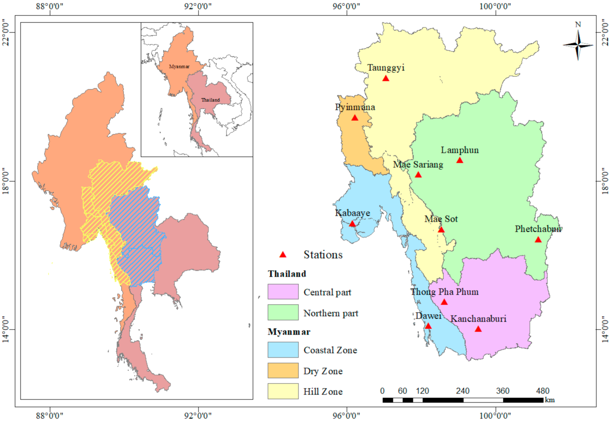
2.1. Site Description

At the beginning, this study collected the daily maximum, mean and minimum temperature from 30 observation stations in Myanmar and Thailand. However, only the data from ten meteorological stations were used in this research based on data quality and accessibility. Six stations, including Mae Sariang (MSR), Lamphun (LPH), Mae Sot (MST), Phetchabun (PCB), Thong Pha Phum (TPP) and Kanchanaburi (KCB) are located in Thailand, while the remaining four stations, namely Taunggyi (TGI), Pyinmana (PMN), Kabaaye (KBA) and Dawei (DWI) are situated in Myanmar. Myanmar is located between 9°32′ N to 28°31′ N latitude and 92°10′ E to 101°10′ longitude [19]. The physical characteristics and topography of Myanmar can be classified into three main agro-ecological zones: the central dry zone, the coastal zone, and the hilly zone [18]. On the other hand, Thailand lies in the tropical zone between latitudes 5°37′ N to 20°27′ N and longitude 97°22′ E to 105°37′ E. According to the climate pattern and meteorological conditions, Thailand can be divided into five regions, namely the northeastern, northern, central, eastern, and southern parts [20]. In general, the selected stations can be defined by three portions i.e., southern, central, and northern of the study area. Each portion of the selected stations is nearly the same in Latitude (°N). The map of the study area and the distribution of the meteorological stations are shown in Figure 1, while the detailed information of the selected meteorological stations is provided in Table 1.

2.2. Temperature Data

The observed data of daily maximum, mean, minimum temperatures during 1990–2019 were collected from the Department of Meteorology and Hydrology (DMH) of Myanmar and the Thai Meteorological Department (TMD). On the other hand, the hourly ERA5 reanalysis data were obtained from European Centre for Medium Ranges Weather Forecast (ECMWF), which provides the data from 1979 to the present. ERA5 is the latest generation of ECMWF atmospheric reanalysis published data that have been released since 2016 with better hourly temporal resolution and spatial resolution compared with the previous products of ERA-Interim [21]. At each meteorological station, the hourly ERA5 temperature data were extracted by a bilinear interpolation method [4,22]. The daily and monthly values of mean, maximum, and minimum values were then aggregated from the hourly values.
The collected raw data of the selected stations may contain inhomogeneities and discontinuities in the time series that could influence the climate trend [18,23]. Therefore, all data were processed for quality control and homogeneity checks to avoid inconsistencies [24]. The most commonly used objective approaches to check data quality before analysis include temporal and spatial outlier checks, interpolation of missing data, and homogeneity tests [25,26]. In this study, all these approaches were performed using R-based packages of RClimDex and RHtestV4. A temporal outlier was determined based on the sample distribution of each calendar month separately for each station [23]. The spatial outlier checking was determined by linear regression between the candidate stations and the nearest neighbour stations for each calendar month [25]. All outliers identified from the temporal and spatial checks were considered as the missing values, and therefore, the linear interpolation method from R programming was used to interpolate and fill in the missing values. The maximum missing data was found to be about 2% for the MST and MSR stations, while the remaining stations were less than 1%. Moreover, a homogeneity check was performed using the RHtestV4 package [26]. Based on extensive quality control and homogeneity checks, the temperature data were calculated to annual anomalies during the 30-year period (1990–2019). To ensure the reliability of the ERA5 data, these data were evaluated by comparing the anomalies with the observations, and their correlations were analyzed.

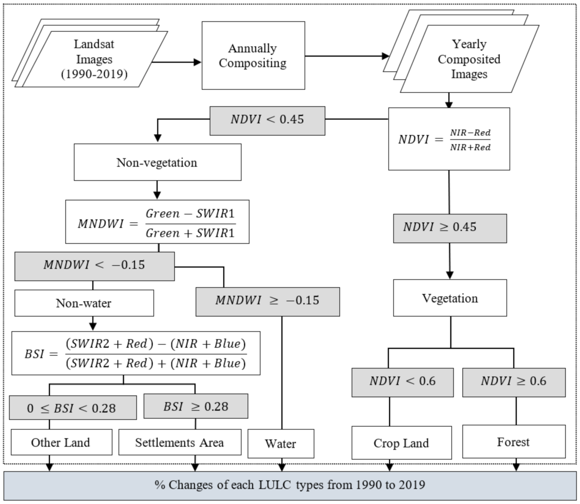
2.3. LULC Classification

2.3.1. Annual Composite Generation

LULC datasets were derived from the Landsat data, the longest and most informative source of earth observation with a medium-high spatial resolution of 30 m [27]. The thirty years (1990–2019) of Landsat surface reflectance data which have been corrected for atmospheric, reflectance, topographic, and satellite sensor effects from Google Earth Engine (GEE) were collected for this study [28]. Then, the total collected images were cleaned off clouds, cloud shadows, and pixels by using the multi-year image synthesis and cloud mask methods available in GEE to obtain the composite data [29]. The annual composite data becomes a single image per year, well suited for time series classification [28]. Finally, the composite image of each year was ready to classify LULC changes in the next steps.

2.3.2. Derivation of LULC

The classification approach used in this study is based on a decision tree algorithm for LULC patterns detection. Figure 2 illustrates the workflow of the LULC classification procedure using three spectral indices; Normalized Difference Vegetation Index (NDVI), Modified Normalized Difference Water Index (MNDWI), and Bare Soil Index (BSI). The NDVI is one of the most widely used remote sensing vegetation indices and has been widely used to identify vegetation based on spectral values [30]. The LULC was first divided into vegetated and non-vegetated areas based on the NDVI value. Forest and cropland were then separated based on their differences in vegetation fraction and growth under vegetated class. In the second step, a hybrid method was used by adding MNDWI within the non-vegetation class to separate water and non-water. The MNDWI can highlight open water features while efficiently suppressing and even removing built-up areas and vegetation and soil noises [31]. Bare land and settlements are notorious as those land cover types hard to separate due to spectral similarities [32]. Therefore, settlement areas and other land uses were separated from non-water using the BSI value. The BSI has mainly been used in forest research to distinguish bare soil and other land cover types, but has also been used for mapping and monitoring bare soil areas [33]. After assigning the index values to distinguish land cover types, the visualization was also interpreted and adjusted to reduce misclassification. The consideration of each LULC category is described in Table 2 [34].
Note: Red: visible red wavelength, Green: visible green wavelength, Blue: visible blue wavelength, NIR: near infrared, and SWIR: shortwave infrared.

2.3.3. Accuracy Assessment

Accuracy assessment was performed using historical high-resolution Google imagery obtained from Google Earth Pro software. Different satellite images collected at the corresponding time were used for accuracy assessment in this study. Specifically, the Google images in 2010, 2012, and 2019 were used for accuracy verification. The total number of verification points was determined for about 400 reference points. They were generated by the random sampling method, and the minimum number of samples of each class was at least 50 points based on the proportion of each LULC type [35,36]. It was assumed that the accuracy validation for the classification method in different satellite images should be sufficient to represent information about the overall accuracy [33]. Finally, the classification accuracy was evaluated using a confusion matrix, and this included user’s accuracy (UA), producer’s accuracy (PA), the overall accuracy (OA), and the kappa coefficient [37]. For the overall results of accuracy assessment at all stations, the minimum value of OA from this study was 80.83%, while the maximum was 87.01%, and the Kappa coefficient was found between 0.75 and 0.83. It revealed that all classified LULC maps achieved relatively high accuracy for further LULC changes analyses [35,38].

2.4. OMR Method for Temperature Trend

Reanalysis datasets are useful for analyzing rapid climate change because they incorporate in-situ measurements, remote sensing observations, and modeled findings in a data assimilation scheme [39]. However, in the data assimilation process, the reanalysis data does not use or has little surface data information, such as surface observations of temperature, moisture, and wind across the land concerning LULC changes [22,40,41]. The surface temperatures are estimated from the atmospheric values [21,42]. Therefore, temperature trends derived from reanalysis data are considered only for large-scale climate change signals resulting from greenhouse gases and atmospheric circulation, but exclude local impacts of LULC changes [22,43,44]. As a result, the reanalysis data should not be sensitives by changes of urbanization and land use effects [7,8,45]. On the other hand, the observed station data include not only local surface forcing such as the effects of LULC changes but also the large-scale atmospheric warming signal resulting from greenhouse effects, natural decadal variability, and volcanoes [5,41]. Therefore, it is able to estimate the effects of LULC changes on surface temperature changes by using a new method of OMR which was introduced by Kalnay and Cai [8]. By isolating near-surface warming from global warming using the OMR approach, which entails subtracting reanalysis data from observed temperature, it is possible to obtain a significant surface climate change signal resulting from various land cover types [4,8,46].
Based on the observation and ERA5 reanalysis data, the annual average temperature anomalies from 1990 to 2019 were calculated in this study. The annual trends of temperature anomalies were calculated using the non-parametric Man-Kendall trend test analysis method [47]. Statistical significance was reported at 95% confidence level. The magnitude of the trend was calculated using Thiel-Sen non-parametric methods based on Kendall’s tau (τ) [48]. Then, the OMR temperature trends were estimated as follows:
TOMR = Tob − Tra
where TOMR is the OMR temperature trends; Tob is the observed temperature trends and Tra is the reanalyzed temperature trends [4]. Finally, this study evaluated the contribution of each LULC type to the warming and cooling based on the correlation coefficient (r) between the OMR trends of temperatures and changes in areas of each LULC type. All correlation coefficients were tested by using a t-distribution with a 95% confidence level.

3. Results

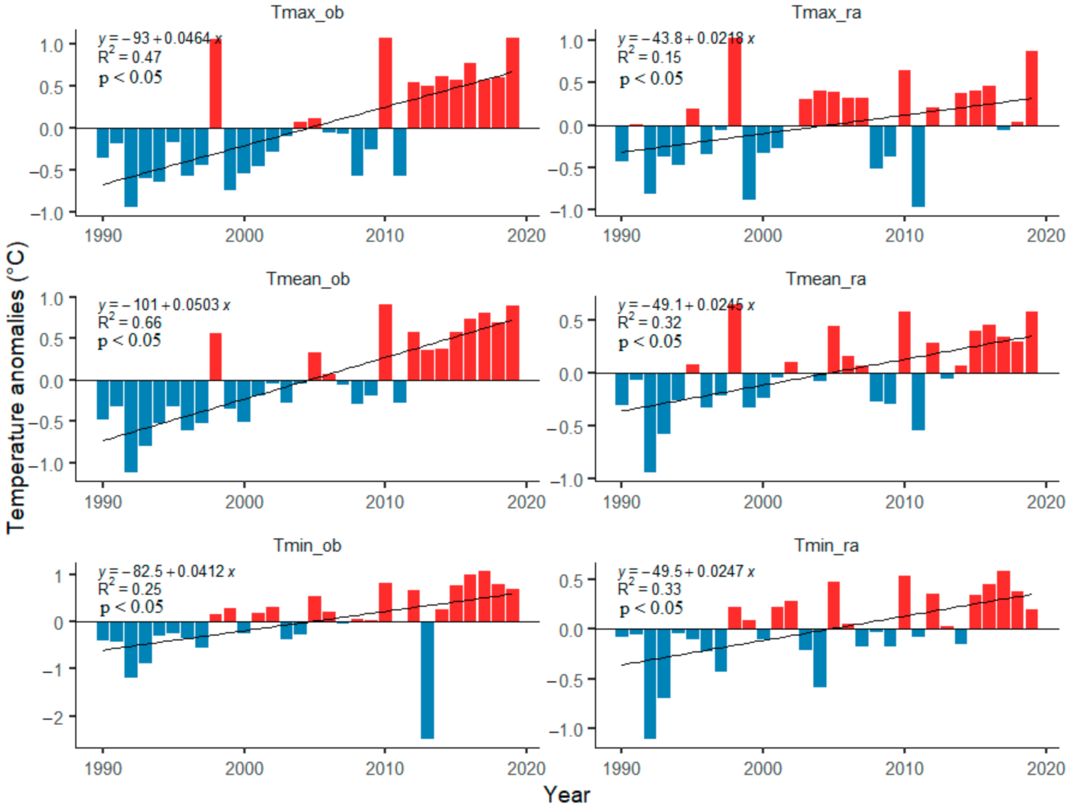
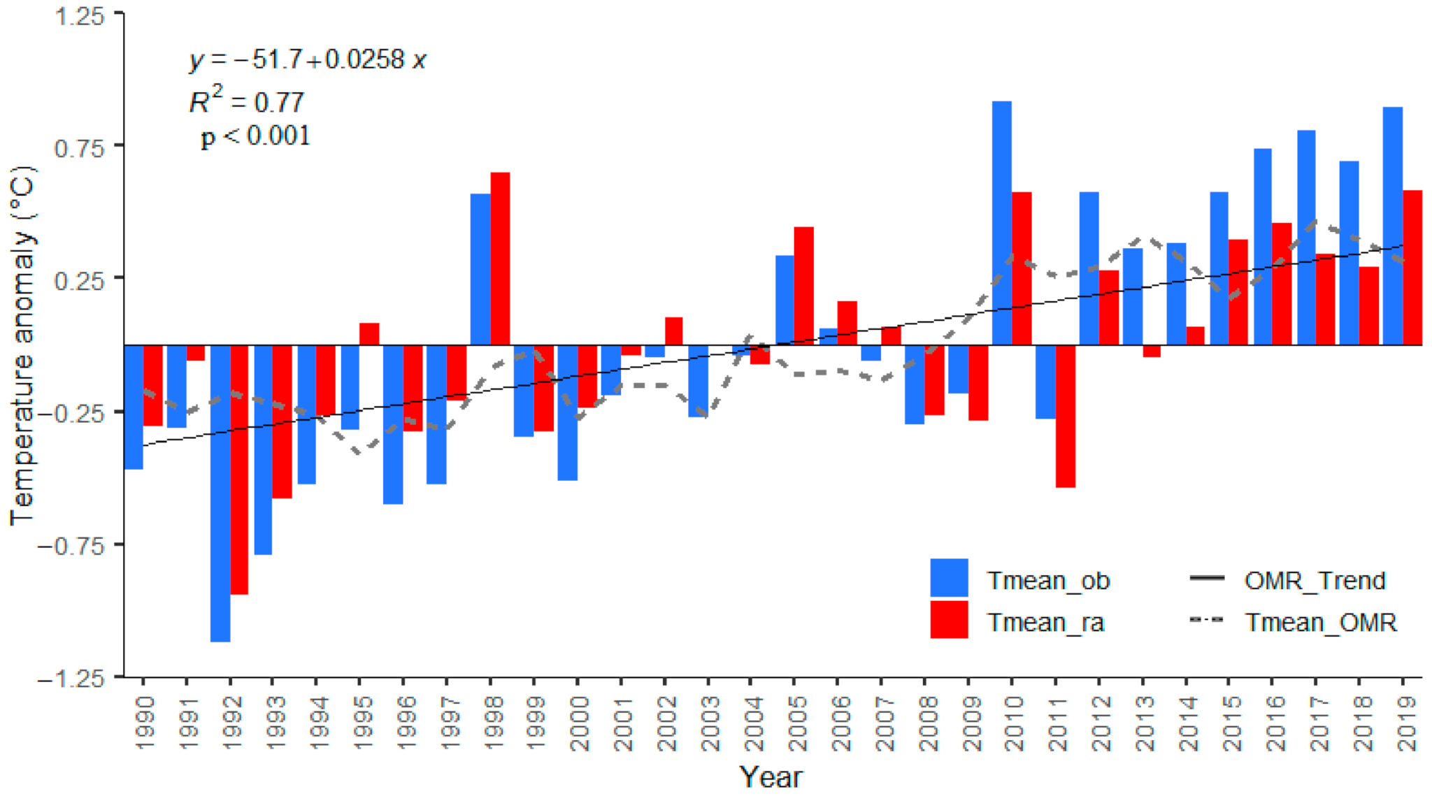
3.1. Relationship between Observation and Reanalysis Data

Generally, the reanalysis data are subject to high uncertainty because of the coarse spatial resolution and assimilation of limited observation [49,50,51]. Therefore, before using in further analysis, consistency check between reanalysis and observation data could provide a basic evaluation for the reliability of both datasets [4,50,51]. In the present study, the mean annual cycles of temperature variables (annual mean, maximum and minimum temperatures) were evaluated and correlations between the ERA5 reanalysis data and the observed data at individual stations were analyzed (Figure 3). Significant correlations were evident between the observed and ERA5 data for the interannual variability, except the minimum temperature (Tmin) for three stations of PMN, KBA and DWI. When the homogeneity test was performed, insignificant change points were detected for the observed data from these three stations. This may explain a weak correlation of Tmin between the observed and ERA5 data at these stations. The maximum and minimum correlation coefficients (r) for the annual mean temperature (Tmean) at PCB and KBA stations were 0.92 and 0.41, respectively.

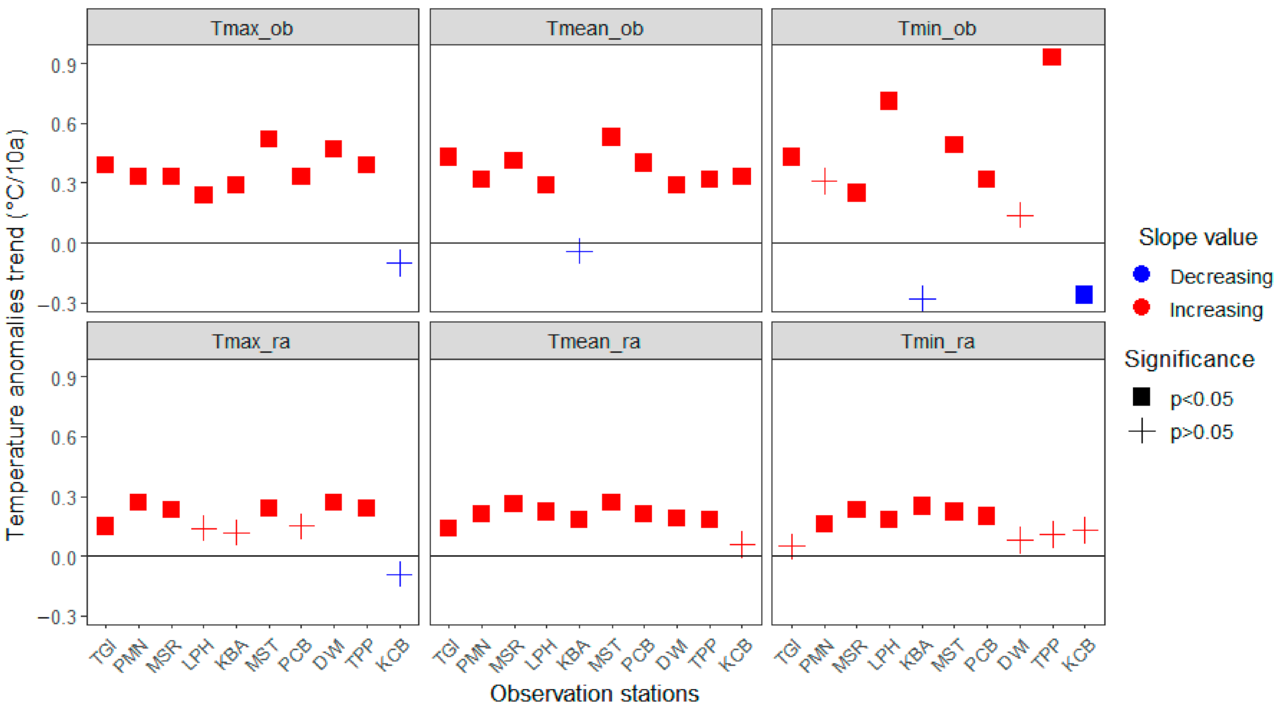
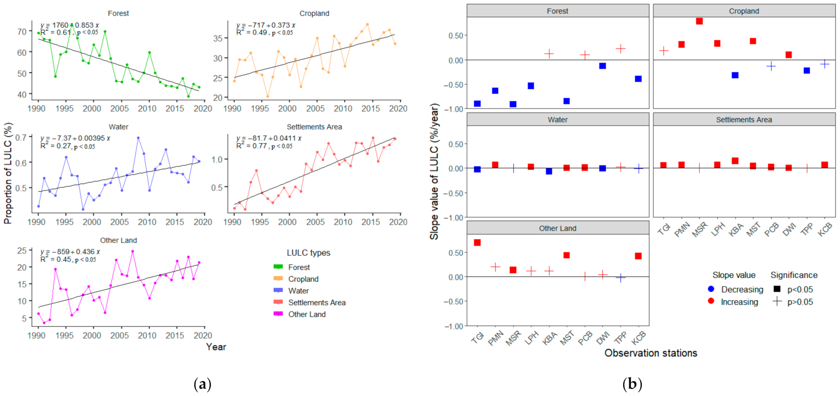
3.2. Temperature Trends

Figure 4 shows the linear trends of the observed and reanalyzed annual maximum, mean, and minimum temperatures anomalies from 1990 to 2019 at the MST station, as an example. The summary results of Mann-Kendall’s Test for all stations are shown in Figure 5. The observed annual maximum temperature (Tmax_ob) had a significant increasing trend at most stations except the KCB station. The increasing trends ranged between 0.24 and 0.52 °C/10a. For the observed mean temperature (Tmean_ob), data from all the stations indicate significant warming trends except at the KBA station. The Tmean_ob ranged between 0.29 and 0.53 °C/10a. The highest increasing trend was detected in the observed annual minimum temperature (Tmin_ob), ranging from 0.25 to 0.93 °C/10a.
The reanalyzed annual maximum temperatures (Tmax_ra) show significant trends in many stations with the range between 0.15 and 0.27 °C/10a. A significant increasing trend of the reanalyzed annual mean temperature (Tmean_ra) was found at all stations with a range between 0.14 and 0.27 °C/10a. For the reanalyzed annual minimum temperature (Tmin_ra), most of the stations show a significant increasing trend in the range of 0.16 and 0.25 °C/10a.
The highest significant increasing trend for the observed temperature was found in the minimum temperature at TPP station by 0.93 °C/10a, while KCB station shows a significant decrease by −0.26 °C/10a. On the other hand, the highest significant increasing trend of the reanalysis data was observed in the maximum temperature at DWI station by 0.27 °C/10a. It is revealed that the observed temperatures showed a higher warming trend than the reanalyzed temperatures.

3.3. Analysis of LULC Changes

3.3.1. Determination of LULC Areas to Be Included in the Analysis

Previous studies indicated that the temperature profiles recorded at a given meteorological station are mainly related to the changes of LULC within a 10 km radius around that station [52]. In order to investigate the uncertainty induced by radius size setting, various radii were tested. Therefore, to determine the land use boundary that will be included in the analysis of the relationship between LULC changes and temperature observation at a selected station, LULC changes for each 1 km radius interval up to 50 km from the meteorological station were estimated. Specifically, the changes of LULC for the initial year (1990) and final year (2019) were quantified for each 1 km increase in radius from the observed station. The results of using this approach are presented in Figure 6.
Generally, it was observed that forest land and cropland were the most dominant LULC categories for both years. The initial shift in forest areas was found around 3 km from the observation station, and its proportion around the observation station gradually increased as the distance from the station increased. The changes of cropland between two years were found around 5 km. On the other hand, the analysis revealed that the water area presented only a small LULC fraction within 50 km around the station. Water areas significantly changed from the first kilometer, except at the TGI that showed changed after 10 km. For the settlement, its areas gradually decreased with increasing distance from the station, and most of the changes between the two years were found before 30 km. Other land uses type also decreased gradually when the distance from the station increased, except at the TGI and KBA stations, where the fractions were relatively constant along 1–50 km radii.
Although a significant starting change of each LULC type between two years was found in various distances around the observation station, most of the changes were detected between 5 km and 20 km. Therefore, a 20-km radius from observation stations was set to study the relationships between LULC changes and land surface air temperature. This is well within the ranges of suggested radius (0.4 to 30 km) for the impact study of LULC on air temperatures at a given meteorological station [52,53,54].

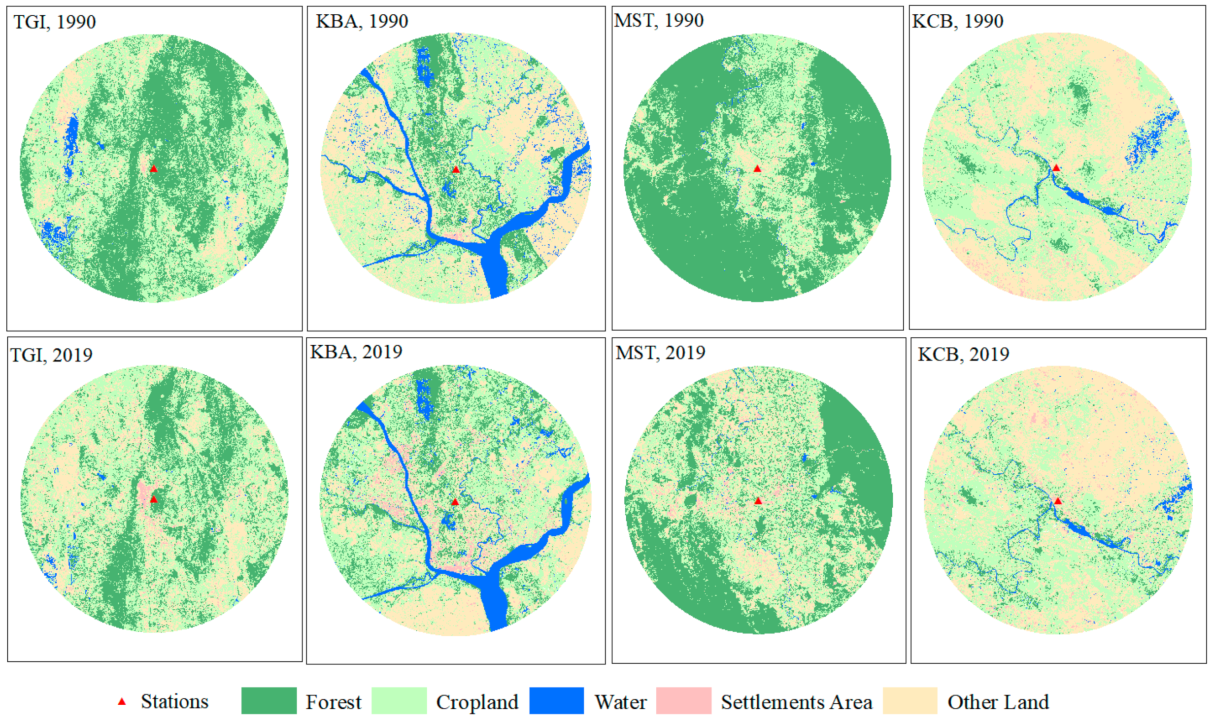
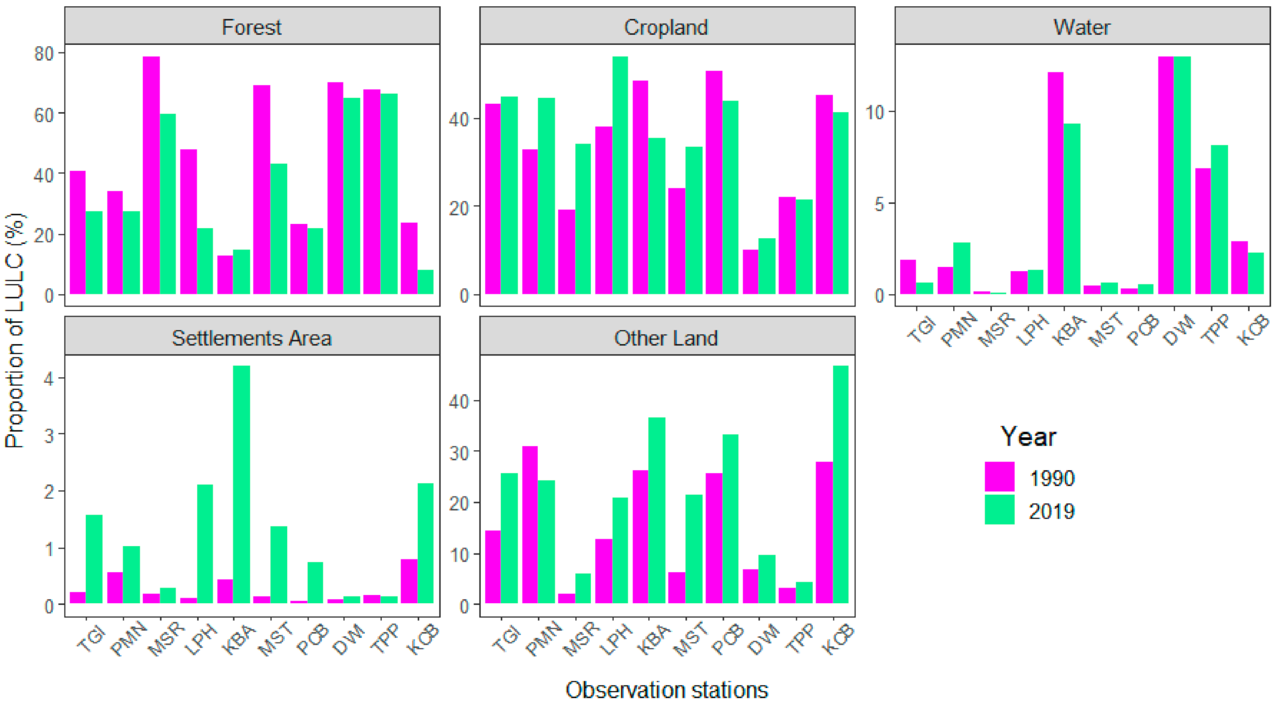
3.3.2. LULC Changes from 1990 to 2019

As discussed in the previous section, the analysis of changes in land use in the 1990–2019 period was conducted inside a 20 km radius (1256 km2) around each observation station (Figure 7). It was found that the dominant LULC types were forest land, cropland, and other land cover types for most of the stations, while water body and settlements area were not much contributed within 20 km (Figure 8). The results of long-term changes in LULC from 1990–2019 are shown in Figure 9a as an example for one typical station and in Figure 9b for every station. The forest land had the most significant decreases compared to other types of LULC at most of the stations. The decreasing range was between −0.13 and −0.92% per year. The highest decrease of forest land from 47.94% in 1990 to 21.58% in 2019 was detected at the LPH station. The MST station also had a high proportion of forest area reduction, from 69.06% in 1990 to 43.16% in 2019. For cropland, a significant increasing trend from +0.09 to +0.78% per year was detected at five stations. However, at the stations of TPP and KBA, it was decreased at the rate of −0.23 and −0.32% per year. On the other hand, cropland around the KBA station had the highest decreasing rate from 48.44% in 1990 to 35.57% in 2019, while at the LPH station, it increased from 37.93% to 54.04%.
There was not much change in the water body, partly because the percentages of water coverage were very small compared to the areas of all other lands. The ranges of water area changes were from +0.008 to +0.069% per year for some stations, and at three stations of DWI, TGI and KBA it showed a significant decrease of −0.01, −0.02 and −0.06% per year, respectively. The high rate changes of the water body was detected at the KBA station by decreasing from 12.11% to 9.30%, while at the TGI station, it declined from 1.86% to 0.58%.
At most stations, significant increases in settlements area from 1990 to 2019 were observed, with ranges from +0.001 to +0.146% per year. The highest increasing rate of settlements area was evident at the KBA and KCB stations by 0.42% and 0.80% to 4.18% and 2.13%, respectively. For other land uses type, only four stations indicated a significant increase by +0.41 to +0.69% per year. Among them, the KCB and MST stations had the highest increases from 27.96% and 6.28% in 1990 to 46.55% and 21.29% in 2019, respectively.

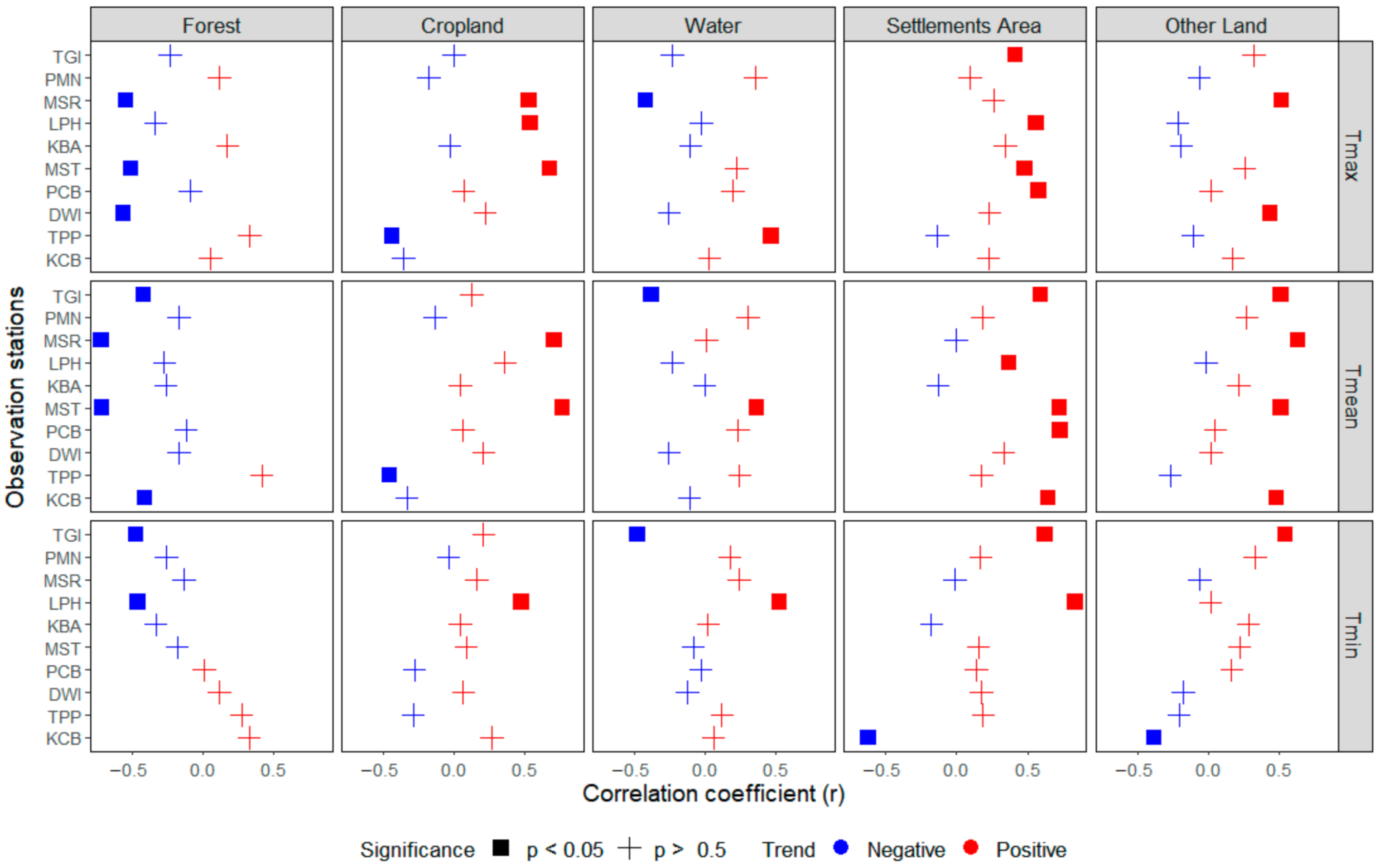
3.4. Analysis of LULC Changes Effects on Surface Air Temperature

Results reported above on variations of temperatures trends observed at stations across the study areas indicate the complexity of factors and their interactions that affect climate at a given location and area. This study has tried to understand the LULC effects on temperatures by analyzing the LULC changes and correlating them to the OMR temperatures at individual meteorological stations. The OMR trend of maximum temperature (Tmax_OMR) showed a significant increase from 1990 to 2019 at most stations with the ranges between 0.10 and 0.24 °C/10a (Figure 10), where the data were subtracted from the observed and reanalyzed values in Figure 11 indicated as an example at one station. The highest significant increasing trend in Tmax_OMR was observed at the MST station. The OMR warming trend for mean temperature (Tmean_OMR) ranged between 0.12 and 0.32 °C/10a. The highest warming trend in Tmean_OMR was found at the KCB station. A significant increase in the OMR trend of minimum temperature (Tmin_OMR) was found in some stations with ranges between 0.10 and 0.81 °C/10a. Only at the KCB station showed a significant decreasing trend by −0.43 °C/10a. Moreover, the correlation coefficients provided in Figure 12 indicate negative impacts of losing forest land and positive impacts of settlements and other land increases on the OMR trends.

4. Discussions

4.1. Contribution of LULC Changes to Maximum Temperature

The relationship between LULC changes and maximum temperature varied among the meteorological stations. It is noted that only those stations with the significant changes at a confidence level of 95% were included in the discussion here. The MSR station found the highest decreasing forest cover rate of around −9.16% per decade (Table 3). However, the warming degree here (0.15 °C/10a) was less than that was found at other stations. This could be explained by the fact that forest land was mainly converted to cropland (increased by 7.83%), and that cropland expansion is usually accompanied by cooling [4,5]. At the MST station, the forest cover loss rate of around −8.53% was lower, but the increasing rate of cropland was also lower (3.73%) than at MSR station. Here the effects of losing forest cover on warming were more obvious (0.24 °C/10a). In addition, it is noteworthy that at TPP station decreases in cropland fraction could contribute to the warming of the maximum temperature (0.16 °C/10a). At DWI station, only forest cover had a high contribution to warming. Even a small fraction of forest areas was decreased here. Settlement areas also contributed to warming temperature; the highest increasing rate of settlements area was found at LPH station of around 0.70%, but its contribution to temperature was lower than at other stations. This was because of the cooling effects of cropland expansion and waterbody, as explained above. On the other hand, the increasing rate of settlements area at TGI station was higher than at PCB station. However, its contribution to warming was lower than at PCB because of the differences between mountain and lowland regions. Therefore, based on these findings, if any other types of LULC are converted to cropland, it likely moderates the maximum temperature increases. Otherwise, the changes of forest land to any other land cover types and any land cover converted to settlements area are contributed to warming temperature. This finding is also in line with the previous research, which indicated that converting agricultural land to all land cover types and converting forest land to other land cover types contribute to warming trends, while conversion of all land cover types to agricultural land contributes to cooling trends [5,11].

4.2. Contribution of LULC Changes to Mean Temperature

Similar to the case of maximum temperature, there were cases where changes in mean temperature were related either to changes in only one type of LULC or to the combined effects from various LULC types (Table 4). These combined effects are best demonstrated at TGI stations. Here, reduction in forest and water body, increases in settlements and bare soil fractions lead together to increases in mean temperature of 0.29 °C. Remarkable warming was also observed at KCB station (0.32 °C). Decreases in the forest and increases in settlements area were also evident here at the KCB station. When comparing to MST and MSR stations where the loss rates of forest were higher than KCB and TGI, the contribution to mean temperature was less than those stations because of the higher conversion rate to cropland at MSR and MST stations. In addition, the fraction of other land uses at TGI and KCB was relatively high in comparison to others (Figure 8), and these might also contribute to higher warming here than at other stations, although a small amount of LULC changes was found at PCB, but the warming trend was higher than others because the station is located in the lowland part of northern Thailand. Here, mountains surround it and the topography therefore influences the local temperature as observed in this study. The dry season is also longer (October to April) than others [55,56].

4.3. Contribution of LULC Changes to Minimum Temperature

The estimated changes of minimum temperature induced by LULC changes are provided in Table 5, which were only three stations where LULC changes were significantly correlated with minimum temperature trends. The strongest increase in minimum temperature was found at LPH station. Here the contribution of forest land conversion to other LULC categories was 0.53 °C/10a. However, the highest rate of forest changes was found at TGI station, but the contribution to minimum temperature was lower than LPH station by 0.14 °C/10a. In detail, the fraction of other lands, especially bare soil, was high, which might reduce the night-time temperature or minimum temperature because the most daily minimum temperature is happening at night. In addition, this study noticed a significant increase in bare soil fraction around 4.18% at KCB station. Here minimum temperature was decreased by −0.43 °C/10a. The cooling effects of bare soil to minimum temperature could be related to night-time radiative cooling, and due to low humidity in areas with bare soil can produce large temperature drops [57]. Broadbent et al. [58] also reported that irrigation of the extremely dry areas (bare soil) could produce large cooling effects because of the bare soil’s great evaporative cooling potential. Besides, paddy fields were mainly cultivated around KCB station, accounting for about 50% of all cropland fractions found in this study [59]. This could also contribute to the cooling at KCB through such evaporative cooling.

4.4. Effects of LULC on Regional Temperature Changes

The rapid socio-economic developments such as increasing infrastructure development in Myanmar and Thailand have led to dramatic land cover changes, mainly deforestation and urbanization [13]. In addition, extreme climate episodes such as extremely high temperatures have been observed in recent years [18,60]. However, comprehensive investigation on the characteristics of changes and the contribution from LULC changes to surface air temperature in this region is still limited. Therefore, this study assessed the changes of near-surface air temperatures in association with the LULC changes.
As indicated at various station sites and temperature parameters, this study found changes in temperatures and LULC during 1990–2019 resulted in different rates of warming and cooling across the study area. The main findings of OMR trends on the averages of maximum, mean, and minimum temperatures were the increases with the rates of 0.17, 0.20, and 0.42 °C/10a, respectively. Overall, this study revealed that the rates of minimum temperature changes in most of the stations were higher than the maximum temperatures. This study suggests that the temperature changes are related to deforestation and urbanization. Alterations of the land surface through LULC changes has resulted in higher absorption of heat during daytime and this subsequently is released during night-time. Normally, the daily minimum temperature is recorded during night-time, which night-time atmospheres are typically more statically stable than daytime [61]. In addition, at night-time, the difference sensible heat flux is relatively small, and thus the surface air temperature largely depends on the ground heat release [62]. As a result, this research revealed that the minimum temperature was two times warmer than maximum temperature.
The dominant modes of LULC changes were decreases in forest cover, increases in cropland and settlement areas at most of the studied stations. However, the rate of temperature increases induced by forest changes largely depended on the types of LULC to which forest land was converted. For example, the changes of forest to cropland and forest to settlement areas varied in their contributions to temperature trends. It was noticed that the changes of forest land to settlement areas caused the higher warming than the changes of forest to cropland by approximately 0.10 °C/10a. These findings were consistent with the previous studies that explained the conversions of agricultural and forest land to all other land cover types contributed to warming trends, while conversions of all land cover types to agricultural land contributed to cooling trends [11]. Nayak et al. [5] also reported that conversion of small vegetation (e.g., shrub, grassland, and green patches on bare land) to forest and agriculture led to a cooling trend, but conversion of agricultural land to bare soil contributed to the warming trend. Our findings are consistent with those explored by Cao et al. [4] that cropland changes to urban areas showed the highest warming effects. According to the biophysical characteristics, the conversion of forest to other land cover types reduced the uptake of moisture by the canopy and roots. Thus, these changes tend to reduce evaporation and then affect the fluxes of moisture and latent heat from the surface to the atmosphere, leading to an increase in temperature near the surface [4,7,11,63,64].
In fact, LULC change is highly dynamic during the development for residential areas and food production in both agricultural countries such as Thailand and Myanmar. Yet, developments may weigh insightfully about which conversions (i.e., area and land use type) should be considered to minimize the effects on local temperature changes. It is obvious that natural forest needs to be maintained and even conserved to keep the diverse benefits or ecosystem service flows, which are essential for both nature, hazard prevention, and climate regulation as mentioned above.

4.5. Research Limitations and Way Forward

Analyzed results and discussions above indicated that there are a few points that may worth further consideration. Firstly, the OMR interpretation may be limited due to interpolation method inaccuracies and non-climatic biases [5,65]. However, the OMR method has the advantages such as the ability to separate the effects of LULC changes on regional climate. Because there is no simple approach to separate the effects of LULC changes on surface temperature from other drivers, OMR method is still widely used. The OMR-based studies have showed robustness by quantifying climate variability and the influence of LULC changes on surface temperature trends [4,5,8,11,65]. It is recommended that more research is needed at different station sites (Myanmar and Thailand) to investigate and compare the robustness of LULC change influences on temperature trends by using different approaches.
Secondly, our results indicated that using decision tree technique in GEE platform for classification of LULC is also quite satisfying and produces good results. Although there was a small issue with misclassified pixels of urban land and bare soil due to spectral similarities and using of a 30 m spatial resolution satellite data, but the overall capability of GEE to perform the classification is still high. It is also suggested for future research to investigate the LULC changes with other classification algorithms such as random forest, support vector machine, for better accuracy. Besides, Google Earth Pro was used to check the accuracy assessment in this study. However, for future studies, it is recommended to perform field data collection of ground truth points for validation of the accuracy.
Lastly, this study could analyze only ten sites of meteorological station and could focus only on surface air temperature aspects. Further studies should aim to include numbers of the station sites across the regions. Such studies may also investigate the changes of LULC effects on other climate parameters such as relative humidity, wind, and precipitation in order to improve our understanding of LULC effects on local climate conditions and patterns at the same sites used in the current study. This is important because the changes of LULC not only affect temperature but also other climate parameters in the observation station [3,66,67,68,69]. In addition, the different time scales should be examined in future work to capture dynamics of LULC and climate parameters in different seasons (e.g., wet and dry seasons).

5. Conclusions

This study investigated the relationships between LULC changes and near-surface air temperature trends from 1990 to 2019 over the major regions in Myanmar and Thailand. The analysis was based on the OMR method. The results obtained in this study indicated that although there were variations in temperature trends among meteorological stations, such variations could be explained by LULC patterns and LULC changes around the stations. The key findings are summarized as follows:
  • The changes of LULC inside a 20 km radius of the selected observation stations changed significantly, as evident from the loss of forest land and increases in cropland and settlements.
  • As a result, the average surface air temperature during 1990–2019 was warmer by 0.17 °C, 0.20 °C, ad 0.42 °C/10a in the maximum, mean, and minimum temperatures, respectively.
  • The rate of minimum temperature increasing is higher than mean and maximum temperatures. However, the mean and maximum temperatures at most of the stations showed significantly increasing trends than minimum temperature.
  • Overall analysis indicates that the reduction of areas under vegetation types (forest and cropland) and expansion of settlements area in most of stations were strongly correlated to temperature warming.
  • The effects of forest cover converted to urban land on temperatures are higher than the effects of forest cover changed to cropland.
These findings on the relationships between LULC changes and temperatures suggested that in Myanmar and Thailand, where LULC changes have been rapid in recent years, the effective management of LULC may be possible to mitigate warming of the local near surface air temperature. Additionally, to improve our understanding of the interactions between LULC changes and climate, future studies should include more observed stations available in the whole region, and more climatic parameters such as precipitation, relative humidity, and wind.

Author Contributions

Conceptualization, K.L.Y. and A.C.; methodology, K.L.Y. and A.C.; software, K.L.Y. and C.T.N.; validation, K.L.Y.; formal analysis, K.L.Y., C.T.N. and A.C; writing—original draft preparation, K.L.Y.; writing—review and editing, K.L.Y., A.C., A.L., P.V. and C.T.N.; supervision, A.C. All authors have read and agreed to the published version of the manuscript.

Funding

The research and studentship of K.L.Y. were supported by the Thailand scholarship (Year 2019) from the Office of the Higher Education Commission (OHEC), Ministry of Higher Education, Science, Research and Innovation (MHESI) and King Mongkut’s University of Technology Thonburi (KMUTT) for M.Sc. program (No.: MHESI 0225.5/1440) at the Joint Graduate School of Energy and Environment (JGSEE), KMUTT. Parts of this study were supported by the Program Management Unit for Human Resources & Institutional Development, Research, and Innovation, NXPO [grant number B16F630087].

Institutional Review Board Statement

Not applicable.

Informed Consent Statement

Not applicable.

Data Availability Statement

Not applicable.

Acknowledgments

The authors are grateful for support from OHEC, JGSEE, and Centre for Climate Change Technology and Innovation, King Mongkut’s University of Technology Thonburi (KMUTT). Special thanks to the data providers of GEE platform, Google Earth, ECMWF, TMD (via. Charoon Laohalertchai, Thailand) and DMH (Myanmar). Our gratitude extends to Kyu Kyu Sein and Nang Phyu Phwe for data collection in Myanmar. Thanks to Mana Raj Rai for sharing knowledge on data analysis. We would like to thank the reviewers for providing valuable feedback and suggestions.

Conflicts of Interest

The authors declare no conflict of interest.

References

  1. Qu, F.; Cui, X.; Yan, H.; Ma, E.; Zhan, J. Impacts of land cover change on the near-surface temperature in the North China plain. Adv. Meteorol. 2013, 2013, 1–12. [Google Scholar] [CrossRef]
  2. IPCC. Summary for policy maker. In Climate Change and Land: An IPCC Special Report on Climate Change, Desertification, Land Degradation, Sustainable Land Management, Food Security, and Greenhouse Gas Fluxes in Terrestrial Ecosystems; Shukla, P.R., Skea, J., Buendia, E.C., Masson-Delmotte, V., Pörtner, H.-O., Roberts, D.C., Zhai, P., Slade, R., Connors, S., Diemen, R., et al., Eds.; Intergovernmental Panel on Climate Change: Geneva, Switzerland, 2019; ISBN 978-92-9169-154-8. [Google Scholar]
  3. Gogoi, P.P.; Vinoj, V.; Swain, D.; Roberts, G.; Dash, J.; Tripathy, S. Land use and land cover change effect on surface temperature over Eastern India. Sci. Rep. 2019, 9, 1–10. [Google Scholar] [CrossRef] [Green Version]
  4. Cao, W.; Huang, L.; Liu, L.; Zhai, J.; Wu, D. Overestimating impacts of urbanization on regional temperatures in developing megacity: Beijing as an example. Adv. Meteorol. 2019, 2019, 1–15. [Google Scholar] [CrossRef]
  5. Nayak, S.; Mandal, M. Examining the impact of regional land use and land cover changes on temperature: The case of Eastern India. Spat. Inf. Res. 2019, 27, 601–611. [Google Scholar] [CrossRef]
  6. Nayak, S.; Maity, S.; Singh, K.S.; Nayak, H.P.; Dutta, S. Influence of the changes in land-use and land cover on temperature over Northern and North-Eastern India. Land 2021, 10, 52. [Google Scholar] [CrossRef]
  7. Lim, Y.K.; Cai, M.; Kalnay, E.; Zhou, L. Observational evidence of sensitivity of surface climate changes to land types and urbanization. Geophys. Res. Lett. 2005, 32, 1–4. [Google Scholar] [CrossRef] [Green Version]
  8. Kalnay, E.; Cai, M. Impact of urbanization and land-use change on climate. Nature 2003, 423, 528–531. [Google Scholar] [CrossRef]
  9. Nuñez, M.N.; Ciapessoni, H.H.; Rolla, A.; Kalnay, E.; Cai, M. Impact of land use and precipitation changes on surface temperature trends in Argentina. J. Geophys. Res. Atmos. 2008, 113, 1–11. [Google Scholar] [CrossRef] [Green Version]
  10. Nayak, S.; Mandal, M. Impact of land use and land cover changes on temperature trends over India. Land Use Policy 2019, 89, 104238. [Google Scholar] [CrossRef]
  11. Fall, S.; Niyogi, D.; Gluhovsky, A.; Pielke, R.A.; Kalnay, E.; Rochon, G. Impacts of land use land cover on temperature trends over the continental United States: Assessment using the North American Regional Reanalysis. Int. J. Climatol. 2010, 30, 1980–1993. [Google Scholar] [CrossRef] [Green Version]
  12. Nguyen, C.T.; Nguyen, D.T.H.; Phan, D.K. Factors affecting urban electricity consumption: A case study in the Bangkok Metropolitan Area using an integrated approach of earth observation data and data analysis. Environ. Sci. Pollut. Res. 2021, 28, 12056–12066. [Google Scholar] [CrossRef]
  13. Yasmi, Y.; Durst, P.; Haq, R.U.; Broadhead, J. Forest Change in the Greater Mekong Subregion (GMS): An Overview of Negative and Positive Drivers; The Food and Agriculture Organization of the United Nations (FAO): Bangkok, Thailand, 2017; ISBN 9789251099117. [Google Scholar]
  14. Pielke, R.A.; Pitman, A.; Niyogi, D.; Mahmood, R.; McAlpine, C.; Hossain, F.; Goldewijk, K.K.; Nair, U.; Betts, R.; Fall, S.; et al. Land use/land cover changes and climate: Modeling analysis and observational evidence. WIREs Clim. Chang. 2011, 2, 828–850. [Google Scholar] [CrossRef]
  15. Kiguchi, M.; Takata, K.; Hanasaki, N.; Archevarahuprok, B.; Champathong, A.; Ikoma, E.; Jaikaeo, C.; Kaewrueng, S.; Kanae, S.; Kazama, S.; et al. A review of climate-change impact and adaptation studies for the water sector in Thailand. Environ. Res. Lett. 2021, 16, 2–33. [Google Scholar] [CrossRef]
  16. Limjirakan, S.; Limsakul, A. Observed trends in surface air temperatures and their extremes in Thailand from 1970 to 2009. J. Meteorol. Soc. Japan 2012, 90, 647–662. [Google Scholar] [CrossRef] [Green Version]
  17. Kachenchart, B.; Kamlangkla, C.; Puttanapong, N.; Limsakul, A. Urbanization effects on surface air temperature trends in Thailand during 1970–2019. Environ. Eng. Res. 2020, 26, 200378. [Google Scholar] [CrossRef]
  18. Sein, K.K.; Chidthaisong, A.; Oo, K.L. Observed trends and changes in temperature and precipitation extreme indices over Myanmar. Atmosphere 2018, 9, 477. [Google Scholar] [CrossRef] [Green Version]
  19. DMH. Myanmar Climate Report; Department of Meteorology and Hydrology (DMH), Ministry of Transport and Communication: Naypyitaw, Myanmar, 2017.
  20. TMD. The Climate of Thailand. Available online: https://www.tmd.go.th/en/downloads.php (accessed on 18 May 2021).
  21. Hersbach, H.; Bell, B.; Berrisford, P.; Hirahara, S.; Horányi, A.; Muñoz-Sabater, J.; Nicolas, J.; Peubey, C.; Radu, R.; Schepers, D.; et al. The ERA5 global reanalysis. Q. J. R. Meteorol. Soc. 2020, 146, 1999–2049. [Google Scholar] [CrossRef]
  22. Wang, M.; Yan, X. A comparison of two methods on the climatic effects of urbanization in the Beijing-Tianjin-Hebei metropolitan area. Adv. Meteorol. 2015, 2015, 352360. [Google Scholar] [CrossRef]
  23. Eischeid, J.K.; Baker, C.B.; Karl, T.R.; Diaz, H.F. The quality control of long-term climatological data using objective data analysis. J. Appl. Meteorol. 1995, 34, 2787–2795. [Google Scholar] [CrossRef] [Green Version]
  24. De Jonge, E.; Loo, M.V.D. An Introduction to Data Cleaning with R; Statistics Netherlands: The Hague, The Netherland, 2013; ISBN 1572-0314.
  25. Feng, S.; Hu, Q.; Qian, W. Quality control of daily meteorological data in China, 1951–2000: A new dataset. Int. J. Climatol. 2004, 24, 853–870. [Google Scholar] [CrossRef]
  26. Wang, X.L.; Feng, Y. RHtests V4 User Manual; Climate Research Division Atmospheric Science and Technology Directorate Science and Technology Branch, Environment Canada Toronto: Toronto, ON, Canada, 2013. [Google Scholar]
  27. Viana, C.M.; Girão, I.; Rocha, J. Long-term satellite image time-series for land use/land cover change detection using refined open source data in a rural region. Remote Sens. 2019, 11, 1104. [Google Scholar] [CrossRef] [Green Version]
  28. Xie, Z.; Phinn, S.R.; Game, E.T.; Pannell, D.J.; Hobbs, R.J.; Briggs, P.R.; McDonald-Madden, E. Using Landsat observations (1988–2017) and Google Earth Engine to detect vegetation cover changes in rangelands—A first step towards identifying degraded lands for conservation. Remote Sens. Environ. 2019, 232, 1–16. [Google Scholar] [CrossRef]
  29. Hu, Y.; Dong, Y. Batunacun An automatic approach for land-change detection and land updates based on integrated NDVI timing analysis and the CVAPS method with GEE support. ISPRS J. Photogramm. Remote Sens. 2018, 146, 347–359. [Google Scholar] [CrossRef]
  30. Patil, A.S.; Panhalkar, S.S.; Bagwan, S.; Bansode, S. Impact of land use land cover change on land surface temperature using geoinformatics techniques. Int. J. Res. Anal. Rev. 2018, 5, 550–559. [Google Scholar] [CrossRef] [Green Version]
  31. Xu, H. Modification of normalised difference water index (NDWI) to enhance open water features in remotely sensed imagery. Int. J. Remote Sens. 2006, 27, 3025–3033. [Google Scholar] [CrossRef]
  32. Nguyen, C.T.; Chidthaisong, A.; Kieu Diem, P.; Huo, L.-Z. A modified bare soil index to identify bare land features during agricultural fallow-period in Southeast Asia using Landsat 8. Land 2021, 10, 231. [Google Scholar] [CrossRef]
  33. Diek, S.; Fornallaz, F.; Schaepman, M.E.; de Jong, R. Barest pixel composite for agricultural areas using Landsat time series. Remote Sens. 2017, 9, 1245. [Google Scholar] [CrossRef] [Green Version]
  34. IPCC. Intergovernmental Panel on Climate Change: Good Practice Guidance for Land Use, Land-Use Change and Forestry; Penman, J., Gytarsky, M., Hiraishi, T., Krug, T., Kruger, D., Pipatti, R., Buendia, L., Miwa, K., Ngara, T., Tanabe, K., et al., Eds.; Institute for Global Environmental Strategies (IGES) for the IPCC: Hayama, Japan, 2003; ISBN 4887880030. [Google Scholar]
  35. Alawamy, J.S.; Balasundram, S.K.; Hanif, A.H.M.; Sung, C.T.B. Detecting and analyzing land use and land cover changes in the region of Al-Jabal Al-Akhdar, Libya using time-series Landsat data from 1985 to 2017. Sustainability 2020, 12, 4490. [Google Scholar] [CrossRef]
  36. Stehman, S.V. Sampling designs for accuracy assessment of land cover. Int. J. Remote Sens. 2009, 30, 5243–5272. [Google Scholar] [CrossRef]
  37. Sarkar, A. Accuracy assessment and analysis of land use land cover change using geoinformatics technique in Raniganj Coalfield Area, India. Int. J. Environ. Sci. Nat. Resour. 2018, 11, 25–34. [Google Scholar] [CrossRef]
  38. Fleiss, J.L.; Levin, B.; Paik, M.C. The Measurement of Interrater Agreement. In Statistical Methods for Rates and Proportions, 3rd ed.; John Wiley & Sons: Hoboken, NJ, USA, 2004; ISBN 0471526290. [Google Scholar]
  39. Yu, Y.; Xiao, W.; Zhang, Z.; Cheng, X.; Hui, F.; Zhao, J. Evaluation of 2-m air temperature and surface temperature from ERA5 and ERA-I using buoy observations in the arctic during 2010–2020. Remote Sens. 2021, 13, 2813. [Google Scholar] [CrossRef]
  40. Chao, L.; Huang, B.; Yuanjian, Y.; Jones, P.; Cheng, J.; Yang, Y.; Li, Q. A new evaluation of the role of urbanization to warming at various spatial scales: Evidence from the Guangdong-Hong Kong-Macau region, China. Geophys. Res. Lett. 2020, 47, e2020GL089152. [Google Scholar] [CrossRef]
  41. Lim, Y.K.; Cai, M.; Kalnay, E.; Zhou, L. Impact of vegetation types on surface temperature change. J. Appl. Meteorol. Climatol. 2008, 47, 411–424. [Google Scholar] [CrossRef] [Green Version]
  42. Yang, X.C.; Zhang, Y.L.; Liu, L.S.; Zhang, W.; Ding, M.J.; Wang, Z.F. Sensitivity of surface air temperature change to land use/cover types in China. Sci. China Ser. D Earth Sci. 2009, 52, 1207–1215. [Google Scholar] [CrossRef]
  43. Wang, J.; Feng, J.; Yan, Z.; Qiu, Y.; Cao, L. An analysis of the urbanization contribution to observed terrestrial stilling in the Beijing-Tianjin-Hebei region of China. Environ. Res. Lett. 2020, 15, 034062. [Google Scholar] [CrossRef]
  44. Dee, D.P.; Uppala, S.M.; Simmons, A.J.; Berrisford, P.; Poli, P.; Kobayashi, S.; Andrae, U.; Balmaseda, M.A.; Balsamo, G.; Bauer, P.; et al. The ERA-Interim reanalysis: Configuration and performance of the data assimilation system. Q. J. R. Meteorol. Soc. 2011, 137, 553–597. [Google Scholar] [CrossRef]
  45. Wang, J.; Tett, S.F.B.; Yan, Z. Correcting urban bias in large-scale temperture records in China, 1980–2009. Geophys. Res. Lett. 2017, 44, 401–408. [Google Scholar] [CrossRef] [Green Version]
  46. Wang, Q.; Riemann, D.; Vogt, S.; Glaser, R. Impacts of land cover changes on climate trends in Jiangxi province China. Int. J. Biometeorol. 2014, 58, 645–660. [Google Scholar] [CrossRef]
  47. Mann, H.B. Non-Parametric test against trend. Econometrica 1945, 13, 245–259. [Google Scholar] [CrossRef]
  48. Sen, P.K. Estimates of the regression coefficient based on Kendall’s tau. J. Am. Stat. Assoc. 1968, 63, 1379–1389. [Google Scholar] [CrossRef]
  49. Durai, V.R.; Bhradwaj, R. Evaluation of statistical bias correction methods for numerical weather prediction model forecasts of maximum and minimum temperatures. Nat. Hazards 2014, 73, 1229–1254. [Google Scholar] [CrossRef]
  50. Bhattacharya, T.; Khare, D.; Arora, M. Evaluation of reanalysis and global meteorological products in Beas river basin of North-Western Himalaya. Environ. Syst. Res. 2020, 9, 1–29. [Google Scholar] [CrossRef]
  51. Alidoost, F.; Stein, A.; Su, Z. The use of bivariate copulas for bias correction of reanalysis air temperature data. PLoS ONE 2019, 14, e0216059. [Google Scholar] [CrossRef] [PubMed] [Green Version]
  52. Gallo, K.P.; Easterling, D.R.; Peterson, T.C. The influence of land use/land cover on climatological values of the diurnal temperature range. J. Clim. 1996, 9, 2941–2950. [Google Scholar] [CrossRef] [Green Version]
  53. Steinke, V.A.; de Melo, L.A.M.P.; Melo, M.L.; da Franca, R.R.; Lucena, R.L.; Steinke, E.T. Trend analysis of air temperature in the Federal District of Brazil: 1980–2010. Climate 2020, 8, 89. [Google Scholar] [CrossRef]
  54. Quiñones, A.J.P.; Cordoba, B.C.; Gutierrez, M.R.S.; Keller, M.; Hoogenboom, G. Radius of influence of air temperature from automated weather stations installed in complex terrain. Theor. Appl. Climatol. 2019, 137, 1957–1973. [Google Scholar] [CrossRef]
  55. Choenkwan, S.; Fox, J.M.; Rambo, A.T. Agriculture in the mountains of Northeastern Thailand: Current situation and prospects for development. Mt. Res. Dev. 2014, 34, 95–106. [Google Scholar] [CrossRef]
  56. Kaewkrom, P.; Thummikkaphong, S.; Somnoumtad, T. Population ecology of some important palm species in Phetchabun Province. Kasetsart J.-Nat. Sci. 2007, 41, 407–413. [Google Scholar]
  57. Shen, X.; Liu, B.; Lu, X. Effects of land use/land cover on diurnal temperature range in the temperate grassland region of China. Sci. Total Environ. 2017, 575, 1211–1218. [Google Scholar] [CrossRef] [PubMed]
  58. Broadbent, A.M.; Coutts, A.M.; Tapper, N.J.; Demuzere, M. The cooling effect of irrigation on urban microclimate during heatwave conditions. Urban Clim. 2018, 23, 309–329. [Google Scholar] [CrossRef]
  59. Santiphop, T.; Shrestha, R.P.; Hazarika, M.K. An analysis of factors affecting agricultural land use patterns and livelihood strategies of farm households in Kanchanaburi Province, Thailand. J. Land Use Sci. 2012, 7, 331–348. [Google Scholar] [CrossRef]
  60. Limsakul, A.; Singhruck, P. Long-term trends and variability of total and extreme precipitation in Thailand. Atmos. Res. 2016, 169, 301–317. [Google Scholar] [CrossRef]
  61. Hua, L.J.; Ma, Z.G.; Guo, W.D. The impact of urbanization on air temperature across China. Theor. Appl. Climatol. 2008, 93, 179–194. [Google Scholar] [CrossRef]
  62. Xiao, Z.; Wang, Z.; Pan, W.; Wang, Y.; Yang, S. Sensitivity of extreme temperature events to urbanization in the pearl river delta region. Asia-Pacific J. Atmos. Sci. 2019, 55, 373–386. [Google Scholar] [CrossRef]
  63. Niu, X.; Tang, J.; Wang, S.; Fu, C. Impact of future land use and land cover change on temperature projections over East Asia. Clim. Dyn. 2019, 52, 6475–6490. [Google Scholar] [CrossRef] [Green Version]
  64. Betts, R.A. Biogeophysical impacts of land use on present-day climate: Near-surface temperature change and radiative forcing. Atmos. Sci. Lett. 2001, 2, 39–51. [Google Scholar] [CrossRef]
  65. Wang, J.; Yan, Z.; Feng, J. Exaggerated effect of urbanization in the diurnal temperature range via “Observational minus Reanalysis” and the physical causes. J. Geophys. Res. Atmos. 2018, 123, 7223–7237. [Google Scholar] [CrossRef]
  66. Paul, S.; Ghosh, S.; Oglesby, R.; Pathak, A.; Chandrasekharan, A.; Ramsankaran, R. Weakening of Indian summer monsoon rainfall due to changes in land use land cover. Sci. Rep. 2016, 6, 1–10. [Google Scholar] [CrossRef] [PubMed] [Green Version]
  67. Li, J.; Zheng, X.; Zhang, C.; Chen, Y. Impact of land-use and land-cover change on meteorology in the Beijing-Tianjin-Hebei region from 1990 to 2010. Sustainability 2018, 10, 176. [Google Scholar] [CrossRef] [Green Version]
  68. Li, Y.; Chen, Y.; Li, Z. Effects of land use and cover change on surface wind speed in China. J. Arid Land 2019, 11, 345–356. [Google Scholar] [CrossRef] [Green Version]
  69. Lai, A.; Liu, Y.; Chen, X.; Chang, M.; Fan, Q.; Chan, P.; Wang, X.; Dai, J. Impact of land-use change on atmospheric environment using refined land surface properties in the Pearl River Delta, China. Adv. Meteorol. 2016, 2016. [Google Scholar] [CrossRef] [Green Version]
Figure 1. The study areas and distribution of selected meteorological stations in Myanmar and Thailand.
Sustainability 13 10942 g001
Figure 2. The designed framework of LULC classification. Thresholding values for each spectral index were obtained from a combination of the thresholding method and image interpretation.
Sustainability 13 10942 g002
Figure 3. Correlation between the observed temperature anomalies and the reanalyzed temperature anomalies in selected meteorological observation stations of Myanmar and Thailand. All correlations with a significance at the 95% confidence levels are indicated as single asterisk (*).
Sustainability 13 10942 g003
Figure 4. Observed and reanalyzed annual maximum (Tmax_ob, Tmax_ra), mean (Tmean_ob, Tmean_ra) and minimum temperature (Tmin_ob, Tmin_ra) anomalies at MST station from 1990 to 2019.
Sustainability 13 10942 g004
Figure 5. Summary results of Mann-Kendall Trend test on maximum (Tmax), mean (Tmean) and minimum (Tmin) temperatures of the observed (ob) and reanalyzed (ra) data at all selected stations in Myanmar and Thailand.
Sustainability 13 10942 g005
Figure 6. Proportion of LULC density along the distance 0–50 km away from observation station in 1990 and 2019 at five selected stations. (Note: pink and green lines represent proportion of LULC in 1990 and 2019, respectively. Vertical lines represent the distance where land cover at most stations changed before 20 km).
Sustainability 13 10942 g006
Figure 7. The spatial distribution changes of LULC inside a 20-km radius (1256 km2) at four typical stations where dramatic LULC changes in the year of 1990 and 2019 were detected.
Sustainability 13 10942 g007
Figure 8. Bar plots show LULC proportion around each observed station in 1990 and 2019.
Sustainability 13 10942 g008
Figure 9. (a) An example of annual changes of LULC in different land cover types at MST stations over the past 30 years; and (b) summary of annual trends for all stations over the same period.
Sustainability 13 10942 g009
Figure 10. The statistical results of Mann-Kendall’s test on the anomalies trends of OMR for maximum, mean, and minimum temperature.
Sustainability 13 10942 g010
Figure 11. An example of observation and reanalysis time series on annual mean temperature anomalies (bar chart) and OMR values (line graph) at MST station from 1990 to 2019.
Sustainability 13 10942 g011
Figure 12. Correlation coefficients between proportion of different LULC categories and the OMR trends (Tmax, Tmean, and Tmin) during 1990 to 2019.
Sustainability 13 10942 g012
Table 1. The detailed information of selected meteorological stations included in the current study [19,20].
Stations CodeStations NameLatitude (°N)Longitude (°E)Elevation (m)Geographical Location
Myanmar
48057Taunggyi (TGI)20.4797.031436Hill
48074Pyinmana (PMN)19.4396.13101Dry
48097Kabaaye (KBA)16.4696.1020Coastal
48108Dawei (DWI)14.0698.1316Coastal
Thailand
48325Mae Sariang (MSR)18.1797.93211Northern
48329Lamphun (LPH)18.5799.03296Northern
48375Mae Sot (MST)16.6798.55196Northern
48379Phetchabun (PCB)16.43101.15114Northern
48421Thong Pha Phum (TPP)14.7598.63104Central
48450Kanchanaburi (KCB)14.0299.5328Central
Table 2. Description of LULC classes in this study.
LULC ClassesDescription
Forest All the land is covered with woody vegetation.
CroplandArable and tillage land, and grass land.
WaterLand is covered or saturated by water for all or part of the year.
Settlements AreaAll developed land, including transportation infrastructure and human settlements of any size.
Other LandBare soil, rock, and all unmanaged land areas that do not fall into any of the other four categories.
Table 3. Maximum temperature changes induced by LULC Changes.
StationsChanges of LULC (%/10a)Tmax_OMR (°C/10a)
ForestCroplandWaterSettlements AreaOther Land
TGI−9.103.09−0.250.54 *6.950.15
MSR−9.16 *7.83 *−0.010.021.32 *0.15
LPH−5.373.28 *0.280.70 *1.150.10
KBA1.21−3.23−0.661.461.220.15
MST−8.53 *3.73 *0.040.41 *4.360.24
PCB0.99−1.300.080.19 *0.040.23
DWI−1.34 *0.95−0.100.010.480.19
TPP1.21−2.28 *0.200.01−0.240.16
* Indicates significant correlation between LULC changes and Tmax_OMR trend at a meaningful level of 95%.
Table 4. Quantitative results of mean temperature changes induced by LULC Changes.
StationsChanges of LULC (%/10a)Tmean_OMR (°C/10a)
ForestCroplandWaterSettlements AreaOther Land
TGI−9.10 *3.09−0.25 *0.54 *6.95 *0.29
MSR−9.16 *7.83 *−0.010.021.32 *0.16
MST−8.53 *3.73 *0.04 *0.41 *4.36 *0.25
PCB0.99−1.300.080.19 *0.040.24
DWI−1.340.95−0.100.010.480.12
TPP1.21−2.28 *0.200.01−0.240.15
KCB−3.93 *−0.08−0.080.67 *4.18 *0.32
* Indicates significant correlation between LULC changes and Tmean_OMR trend at a meaningful level of 95%.
Table 5. Quantitative results of minimum temperature changes induced by LULC Changes.
StationChanges of LULC (%/10a)Tmin_OMR (°C/10a)
ForestCroplandWaterSettlements AreaOther Land
TGI−9.10 *3.09−0.25 *0.54 *6.95 *0.39
LPH−5.37 *3.28 *0.28 *0.70 *1.150.53
MST−8.533.730.040.414.360.28
PCB0.99−1.300.080.190.040.10
TPP1.21−2.280.200.01−0.240.81
KCB−3.93−0.08−0.080.67 *4.18 *−0.43
* Indicates significant correlation between LULC changes and Tmin_OMR trend at a meaningful level of 95%.
Publisher’s Note: MDPI stays neutral with regard to jurisdictional claims in published maps and institutional affiliations.

