Application of Macroscopic Fundamental Diagram under Flooding Situation to Traffic Management Measures

Abstract

Bangkok, Thailand is prone to flooding after heavy rain. Many road sections become impassable, causing severe traffic congestion and greatly impacting activities. Optimal vehicle management requires the knowledge of flooding impact on road traffic conditions in specific areas. A method is proposed to quantify urban flood situations by expressing traffic conditions in specific ranges using the concept of macroscopic fundamental diagram (MFD). MFD-based judgement allows for a road manager to understand the current traffic situation and take appropriate traffic control measures. MFD analysis identified traffic flow–density and density–velocity relationships by using the shape of the estimated MFD travel time-series plots. Then, results were applied to develop a traffic model with vehicle-flow parameters as a measuring method for road-network performance. The developed model improved road-network traffic-flow performance under different flood conditions. A method is also presented for traffic management evaluation on the assumption that flooding occurs.

1. Introduction

Global climate change has induced rainfall extremes in terms of frequency, duration, pattern, and intensity in many cities of developing countries [1]. As a result, urban flooding is one of the major challenges due to intensified rainfall events and inadequate urban engineering infrastructures [2,3]. For example, in the Bangkok metropolitan region (BMR), average total annual rainfall measured by the Thai Meteorological Department exceeded 2000 mm and caused road floods. In the BMR, maximal road flood depths are recorded by detectors installed to monitor flood conditions on roads and tunnels, and collect cumulative average rainfall measurements. When average rainfall accumulated at less than 60 mm/h, 14 flooded areas occurred, while rainfall at over 60 mm/h produced 56 flooded areas, which negatively impacted everyday activities [4]. Drivers modify their travel patterns by taking alternative routes, leaving for destinations at different times or canceling the trip altogether. To better understand and minimize the traffic impact of different flood conditions, flood-related data must be integrated with road usage statistics.

The development and implementation of strategies that minimize the effects of adverse flood conditions require comprehensive knowledge of how flood events impact traffic operations, and how best to assess flood-related effects for a given scenario. Previous research integrated flood simulation with traffic analysis to model different viewpoints of the interplay between these two spatiotemporal phenomena [5]. This integration was used to build a road-network model to assign trip paths, consider the effects of road closures, and evaluate travel delays and vehicle volume redistribution in a given flash-flood scenario by considering the influence of floods on mobility, mainly focusing on severe flood conditions. The relationship between flood events and traffic operations was assessed by a traffic simulation model that could handle complex roadway geometrics, traffic control devices, and vehicle configurations.

However, if key parameters within a traffic model could be changed under various flood conditions, this would greatly assist in developing improved flood-responsive traffic management strategies. The MFD or the relationship between traffic density and traffic variables [6] was determined to assess the service level of the road network and serve as a vehicular access control measure in urban areas with complex road networks [7,8]

MFD determinants as the dynamic nature of traffic flow in urban networks were copiously studied [9,10,11,12,13]. Suwanno et al. [14] used precipitation intensity and the number of nonrainy days with Bluetooth-enabled traffic data installed at junctions to analyze the main MFD parameters decreasing in each rain condition. These parameters were applied to the delay function of the static traffic model to measure traffic efficiency. Results showed that increased traffic concentration had significant impact on the flow characteristics of the static traffic model of an urban road network. However, the intensity of the rain affected the shape of the MFD as a weak correlation factor because rainfall alone does not consider fast flow paths and areas where deep puddles completely block the roads. Moreover, using Bluetooth data collection in previous work showed a lack of transportation mode in upstream and downstream traffic, which is able to cut the outlier from only abnormal speed. Probe data are utilized in this study to eliminate this imprecision of the data of mode of transportation and driving speed.

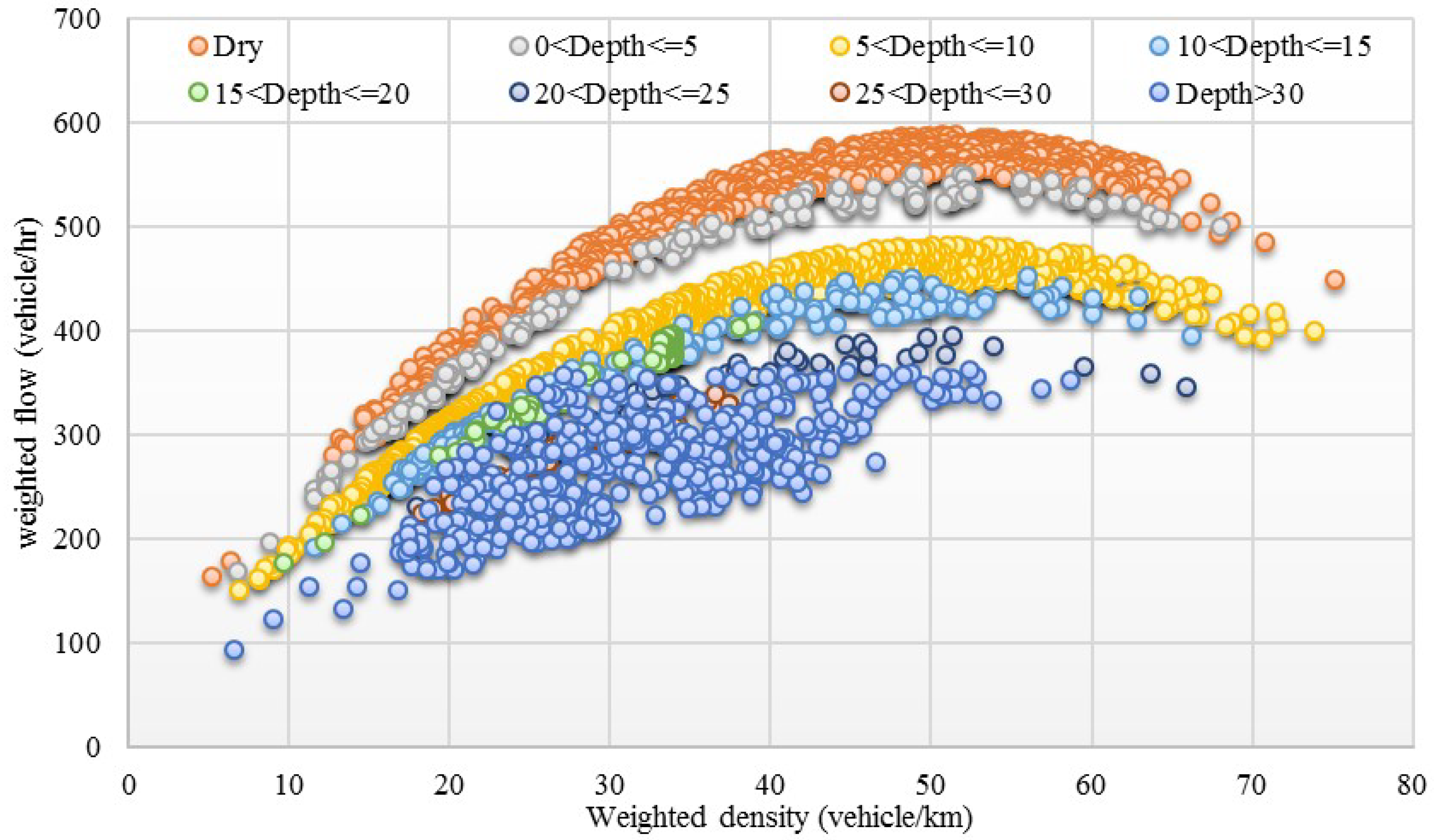
Using the MFD concept, the volume–density relationship of a large network was used to generate a performance diagram and evaluate traffic-flow characteristics. As mentioned by Knoop and Hoogendoorn [15], the Greenshields relationship was used to estimate MFD parameters for road surfaces under varying flood depths. A road-network model was then built to determine optimal travel routes by considering how the effects of road degradation impacted travel delays and vehicle distribution in a given road flood.

An accurate assessment of the impact of different flood conditions on MFD shape has not been previously undertaken for large road networks. The development of empirical relationships between depth of floodwater and vehicle speed reduction cannot analyze impact at the network macroscale that requires the relevant parameters of speed, flow, and density. To resolve this problem, changes in MFD parameters with flood conditions were assessed, and results were applied to generate a traffic model to analyze impact on the whole network. However, this study only considered MFD shape comparisons for a single reservoir. Future investigations should examine flow exchanges in multireservoirs to assess the principle of MFD-based modeling over multiple regions. The main idea is to protect a given area by limiting inflow at its periphery to maintain maximal throughput. In practice, inflow limitation can be achieved by tuning traffic-light timings or road pricing.

2. Data Collection and Extraction

The case study was for the Sukhumvit district, located in the eastern suburban area of Bangkok. This area has high flood risk because it is flat, and the gravity discharge of stormwater takes time. Pumps are used to move water to the main drainage system [16,17].To construct the MFD, taxi data that were collected during 2019 were used as open data (historical raw vehicles and mobile probe data in Thailand) provided by [18]. Data from 5 a.m. to 12 a.m. on weekdays were included in the study with no freeway transport. Only taxis probes occupied by passengers were considered because they reflected the behavior of regular vehicles. In total, 78,078 taxis were recorded as registered in Bangkok in March 2019 [19], and a taxi penetration rate per day of 22.45% was used to estimate the MFDs [20]. The road flood monitoring system monitors flood conditions on roads and underpasses in the Bangkok area [19]. The system collects data at 5-minute intervals. The MS SQL database stores the data for a long time period, making it a very useful tool for road-flood forecasting. A total of 94 sensors were installed on important roads throughout urban Bangkok, with 8 sensors in tunnels to measure and display real-time flood graphs.

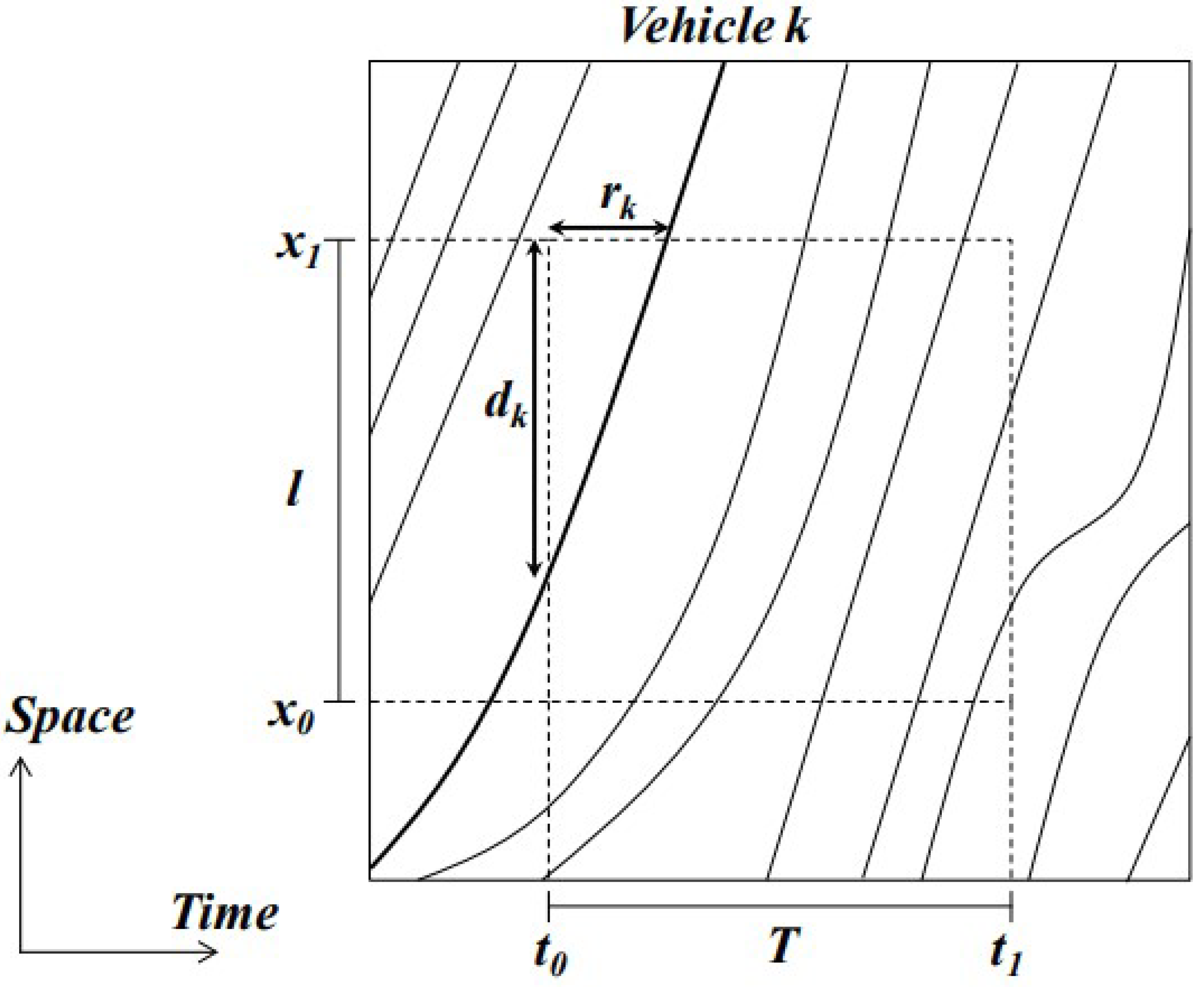
This study estimated the MFD using vehicle trajectories from taxi probes that covered the Bangkok area. A taxi characteristically drives randomly with wide distribution, and the destination is determined by the passengers. This conforms to the characteristics of resident travel and reports their locations as timestamps at every uplink interval. Taxi trajectories were reconstructed on a time–space diagram as shown in Figure 1.

For vehicle trajectories, formulae from Edie’s definitions [21] based on time–space diagram presented in Figure 1 were used to extract average flow (${\overline{q}}_i$) (Veh/h), average density $\overline{k}$ (Veh/km), and average speed $\overline{s}$ (km/h) in the network to obtain the MFD for a rectangular region in time and space with dimensions of length of time intervals (T) and total length of all roads in the network (L). Flow and density were defined on the basis of total distance travelled ($TD{T}_i^{\prime }$) and total time spent ($TT{S}_i^{\prime }$), as shown below for section i.

$$TD{T}_i^{\prime }=\sum _i{d}_{i,k},TT{S}_i^{\prime }=\sum _i{r}_{i,k}$$

(1)

where,

• $d_{i,k}$: distance traveled by vehicle k in section I, and
• $r_{i,k}$: time spent by vehicle k in section i.

Then, flow and density are defined as

$$q_i^{\prime }=\frac{TT{S}_i^{\prime }}{n_i{l}_{i}T},k_i^{\prime }=\frac{TD{T}_i^{\prime }}{n_i{l}_{i}T}$$

(2)

where,

• $q_i^{\prime }$: flow by a vehicle in section i,
• $k_i^{\prime }$: density by a vehicle in section i,
• $n_i$: number of lanes in section i, and
• $l_i$: length of section i.

The flow and density of full traffic are estimated as

$$q_i=\frac{q_i^{\prime }}{X_i},k_i=\frac{k_i^{\prime }}{X_i}$$

(3)

where

• $X_i$: proportion of the number of taxis to full traffic counts in section i.

Lastly, the area average flow (Q) and density (K) are calculated by averaging section variables across an area according to the following equations.

$$Q=\sum _i\frac{q_i{l}_i}{l_i},K=\sum _i\frac{k_i{l}_i}{l_i}$$

(4)

3. MFD Model Results

The relationships in Figure 2 show the MFD shape as a change in the traffic operation of networks under different flood levels. The traffic situation in this area in Thailand is critical traffic jams. Probe data show that average traffic speed is normally about 30 km/h, which generates the maximal traffic volume of about 600 veh/lane/h in dry road conditions. Varying degrees of impact make the MFD shape change, and scatters occur. Dry conditions have different degrees of impact on the stability and certainty of the road network. Flood levels of less than 5 cm only slightly affected the MFD shape change, with clear differences in the MFD shape change for flood levels from 5 to 20 cm. Flood levels exceeding 30 cm had a greater effect on the discrete shape of the MFD. According to the speed–flow–density relationship, flow is the product from speed and density, and can be found from the number of vehicle passing on the reference point. Therefore, flow can be zero when speed and density or both are zero. Density increases to the maximum, which means that vehicles are not moving past the reference point. Thus, flow is decreased after density becomes high.

Table 1. Equation of macroscopic traffic variables.

Depth (cm)	Density-Flow
	Equation	${\mathit{R}}_{\mathit{square}}$
Dry	$y=-0.1968x^2+20.283x+47.39$	0.97
(0, 5]	$y=-0.181x^2+18.749x+51.92$	0.95
(5, 10]	$y=-0.1582x^2+16.342x+41.38$	0.93
(10, 20]	$y=-0.1437x^2+14.988x+43.54$	0.92
(20, 30]	$y=-0.1271x^2+13.528x+18.90$	0.90

shows equations describing the relationships between macroscopic traffic variables under different flooding depths. The R-squared value represents a discrete change in MFD under flood depth. R-squared decreases as flood depth increases, causing continuity to decrease. For smaller R-squared values, MFD shows more discrete changes.

The equation relation in Table 1 was obtained by analyzing and fitting Greenshields’s parameters [6] to represent and evaluate the traffic states of the study network, such as free flow velocity ($u_f$), maximal capacity ($q_c$), and maximal density ($k_j$). Results of the key traffic-flow parameters are presented in

Table 2. Equation of macroscopic traffic variables.

Depth (cm)	Free Flow Speed (km/h)		Maximal Flow (veh/h)		Jam Density (veh/km)
	Value	% Change	Value	% Change	Value	% Change
Dry	36	-	750	-	122	-
(0, 5]	33	−8.3	538	28.3	122	0
(5, 10]	29	−19.4	464	−38.1	126	3.2
(10, 20]	26	−27.7	434	−42.1	121	−0.8
(20, 30]	25	−30.5	378	−49.6	129	+5.7

.

4. Development of the Traffic Model

A dynamic traffic assignment (DTA) model implements a dynamic user equilibrium in the time-dependent nature of demand and network characteristics to produce more realistic traffic conditions on a large scale. Mesoscopic models, on the other hand, capture traffic dynamics in less detail, but are faster and easier to apply and calibrate than microscopic models are. Therefore, they are most suitable for modelling large networks, while microscopic models are usually applied to smaller areas [22].

This study considered a mesoscopic traffic simulation as a dynamic equilibrium-based model to determine a balance between large-scale low-level details in macromodels, and small-scale high-fidelity in micromodels [23]. This model can capture traffic-queue build-up and dissipation across lanes through upstream intersections caused by traffic controls (signals or signs), flow capacity, and lane-changing behavior [23,24,25,26] to generate and track individual vehicles or packets of vehicles. The model assesses the movement of these vehicles according to macroscopic relationships as speed, density, and flow, and considers queuing and spillback due to subject link capacity and downstream link queuing capacity.

Vehicles are simulated at the microscopic level to determine path costs. In these models, the planner specifies the level of detail for vehicles, time, and network inputs. The mesoscopic model consists of the three main elements of traffic demand, network definition, and traffic controls. Traffic demand is represented by a time-dependent origin–destination (OD) matrix for each class of modeled vehicles. The representation of the road network is at the level of individual lanes and includes the definition of turn pockets. The permitted lanes for each intersection movement and lane prohibitions by vehicle class are specified where necessary. The network definition does not require lane width or detailed intersection geometry, such as a turning radius. Traffic controls contain all relevant information regarding the different signaling plans on the intersections.

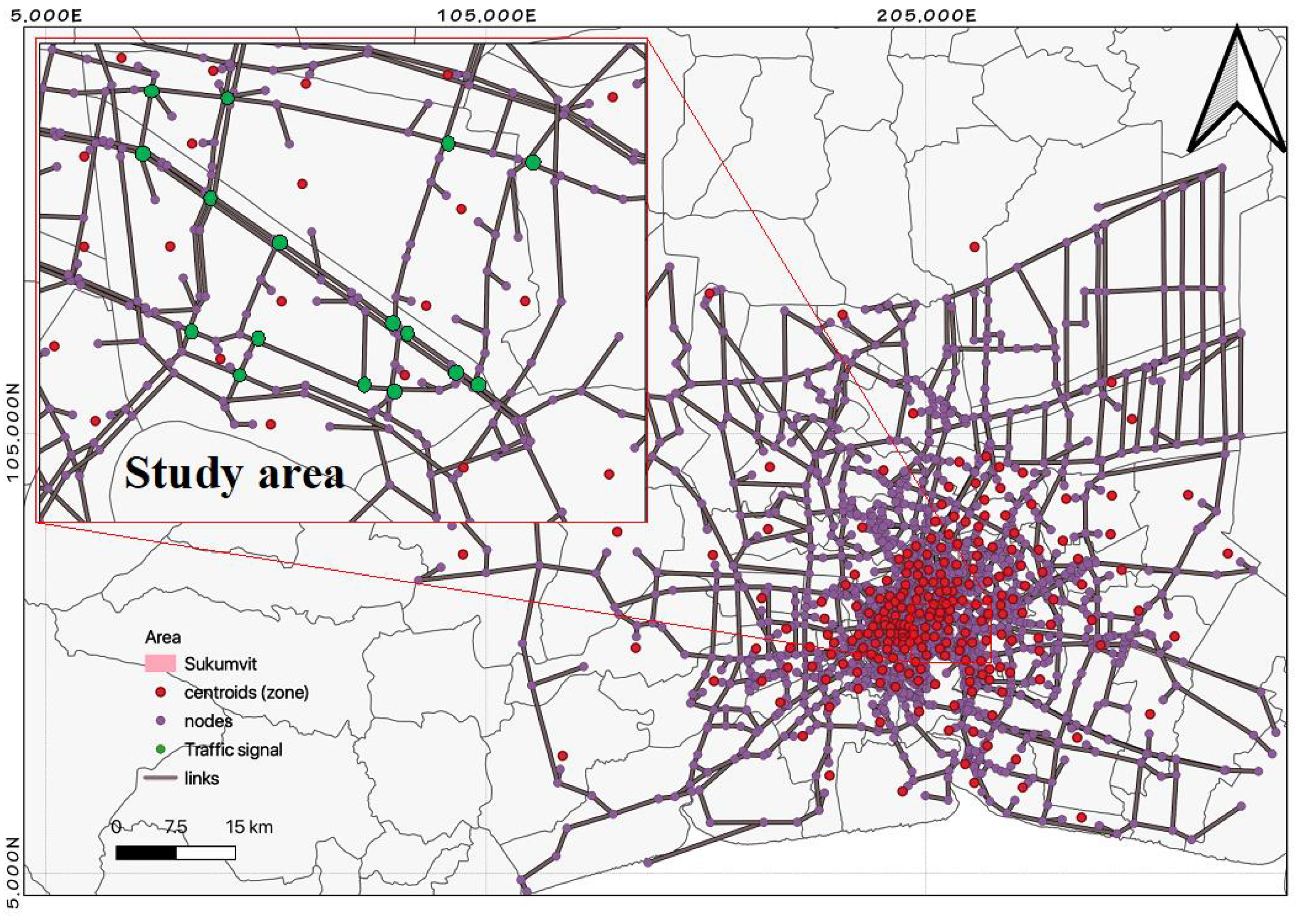
However, the existing Bangkok traffic model, developed in 2017 and called the extended Bangkok urban model (eBUM), is a macroscopic traffic model, developed by the Office of Transport, Traffic Policy, and Planning [27]. Before applying the eBUM model to analyze and forecast transport and traffic situations in the mesoscopic traffic model, we updated the traffic model in 2019 with the most relevant current traffic conditions by using a four-step method. Then, we extracted the road network for the case study of the Sukhumvit area from the updated eBUM model and imported it into a baseline scenario as a new database. The matrix resulting from the transversal assignment was also imported into the new database and used as the demand assigned in the subarea scenario to perform the requisite adjustments. The subarea model consisted of 88 zones, 207 nodes, 766 links, and 16 traffic signals, as shown in Figure 3.

This subarea network was the base scenario for the dynamic model debugging and calibration process. The models simulated the peak hour at full demand, with half an hour for the network to warm up and another half an hour to cool down after peak, with 80% of the peak-hour demand. Vehicles in the model were of the private car class. The model was run with a maximum of 200 iterations and a 1% relative gap. A 15-min assignment interval, equivalent to 8 intervals for each assigned OD matrix, was used. Up to 20 paths were searched in one assignment interval. Simulation results were collected every 15 min after the warm-up period for one hour.

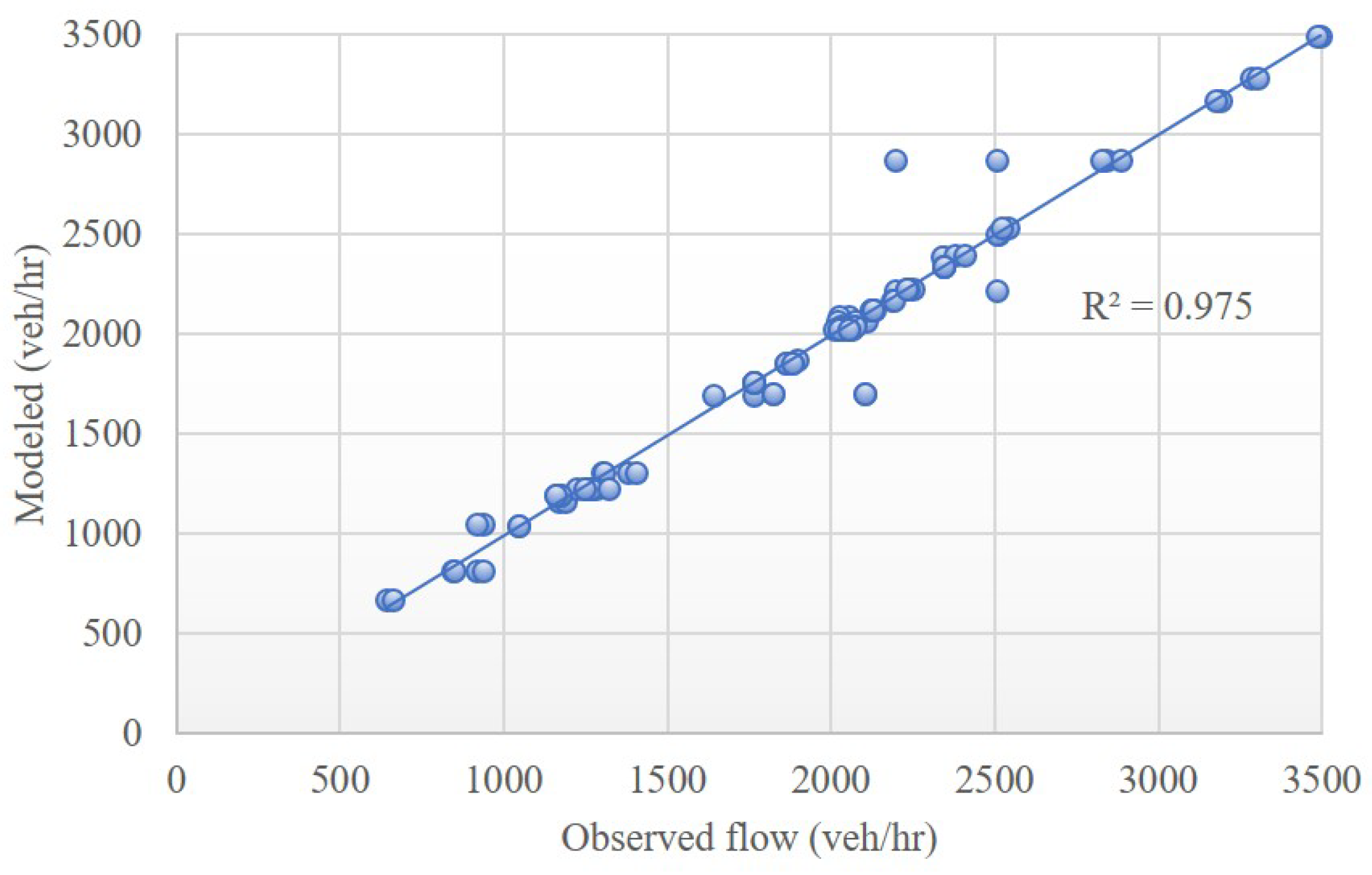
In a DTA model, a relative gap of less than 2% is considered to be good, but is not easily achieved in highly congested networks (Chiu et al., 2010). However, the relative gap only gives an idea of the stability of the current solution and does not quantify the solution with respect to the underlying equilibrium (user-optimal) objective; this indicates that the algorithm is no longer improving the results, but does not indicate how well the final solution satisfies the desired objective of equilibrating travel times on alternative paths. Calibration is required to ensure that the model can replicate traffic volumes, travel times, and other travel patterns in the network. This process involves the calibration of both the demand and supply parts of the model. This was achieved by using model volumes and observed counts at the important road segments in the network.

Figure 4 shows a scatterplot graph that compares model flow and observed flow for the morning peak hours between 7:30 and 8:30. Results indicated that the model was well-calibrated, with $R^2$ of 0.975.

Network simulation results are based on link results aggregated to totals or averages for the entire network, as shown in

Table 3. Network results of the base scenario.

Base Scenario	7:30–7:45	7:45–8:00	8:00–8:15	8:15–8:30
In count (vehicle)	21,414	21,106	20,469	20,773
Out count (vehicle)	19,585	19,087	18,735	18,774
Vehicle hours traveled (VHT)	2620	3076	3529	3833
Vehicle kilometers traveled (VKT)	92,735	91,913	91,662	90,809

, ‘In count’, we measured the number of vehicles that entered the physical space of the network and passed the entrance connectors during the time interval. ‘Out count’ measured the number of vehicles that exited the physical space of the network during the time interval and exited from the exit connectors, and VHT measured the total vehicle hours of travel during the time interval inside the network. This measure did not include waiting time on virtual links, while VKT measured total vehicle kilometers traveled during the interval. As with VHT, this does not include vehicles on virtual links.

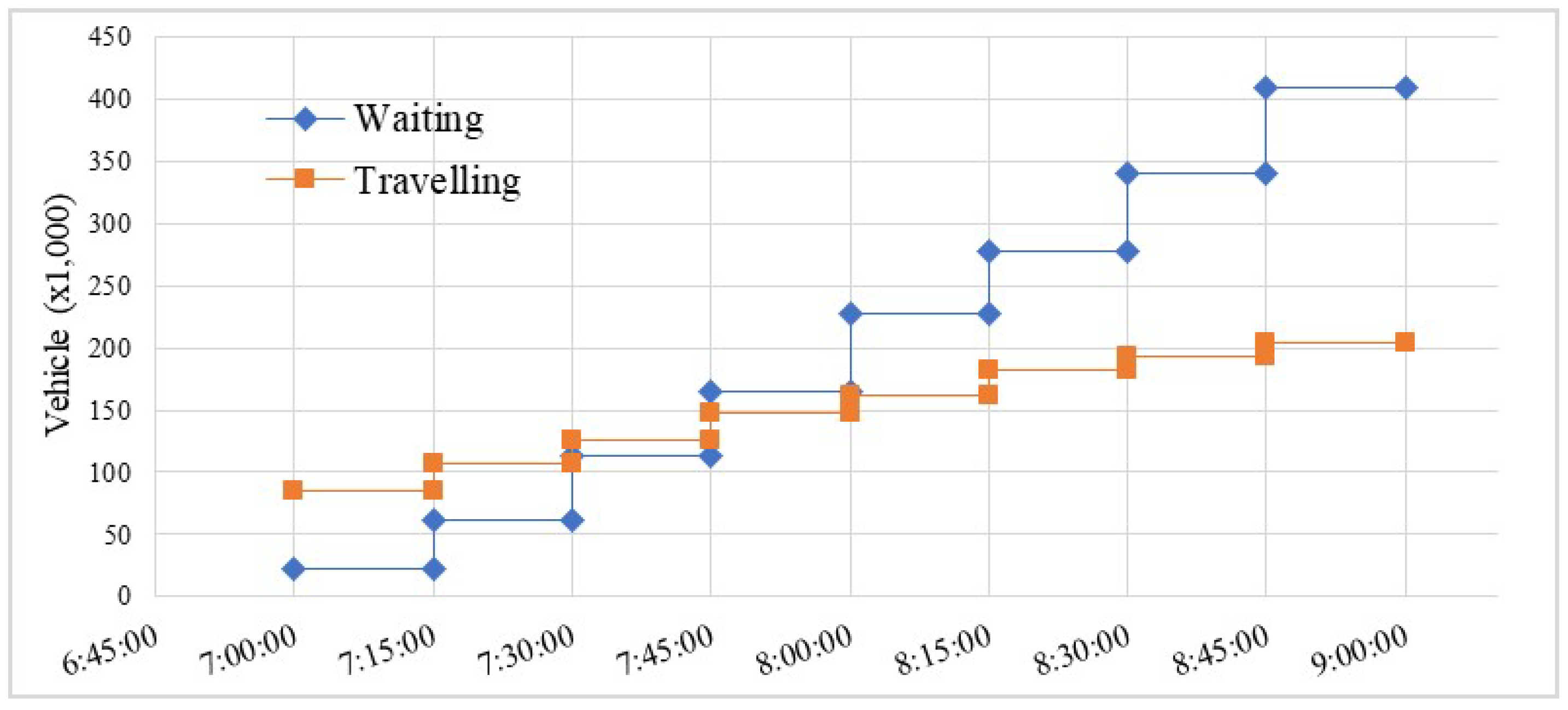
Figure 5 shows the relevant outputs as the number of vehicles waiting to enter the network and the number of vehicles remaining in the network at the end of the simulation. The blue line changed suddenly at the third interval (7:45), reflecting the start of the peak-hour interval until after the last peak interval demand. Over 25,000 vehicles were waiting to enter the road network. These vehicles were stuck on virtual links and could not enter the road network to complete their trips.

Application of MFD Parameters to the Traffic Model

THe systematic consideration of the influence of patterns in a supply and demand structure on a global scale is a requisite for the successful and effective transfer of policy interventions between networks with different structures. Thus, the influence of supply and demand on traffic conditions was investigated. Demand was assessed as the magnitude and distribution of movements of travelers between different locations when aggregated across the geographical area served by a network. The main study interest concerned the performance of the transport system when placed under extreme pressure as an average weekday morning peak period for private cars and assumed that modal travel behavior did not change much during road floods. Supply was assessed as physical infrastructure, composed of roads and intersections, and the capacity to efficiently facilitate the movements of travelers by systematically changing input MFD parameters. Flood depths are displayed in

Table 4. Traffic parameters in traffic model according to flood levels.

Flood Depth (cm)	Remain Performance (%)
	Free Flow Speed	Maximal Flow	Jam Density
0–5	0.92	0.72	1.00
5–10	0.81	0.62	1.00
10–20	0.72	0.58	0.99
20–30	0.69	0.50	1.06

. Maximal flood depth was considered to be 30 cm.

A mesoscopic model was used with three components of traffic flow, as shown below [25]. (1) Car-following models describe the steady-state properties of traffic on a roadway. Steady-state properties can be observed when traffic is moving at a constant speed, and thus also at a constant flow and density. (2) Gap acceptance is the amount of time available for a lower-priority vehicle to execute its movement and clear the point of conflict with a higher-priority vehicle. The relative wait is the difference between the delay that two vehicles incur at an intersection (not including delays due to red traffic signals) as the next vehicles to exit by their respective lanes. This delay is the amount of time spent waiting for acceptable gaps in higher-priority movements. (3) Lane changing is the movement of vehicles on individual lanes of a roadway. How drivers utilize the lanes on the road can significantly impact delays and how these delays propagate through the network. Vehicle trajectories within links are implicitly modeled. Each driver must choose the lane by which to enter and exit a link just before actually arriving at the link. Once onto the link, the choice cannot be reconsidered. The rules used to model drivers’ lane-choice behaviors are complex, combining a look-ahead procedure with local lane-choice rules. The look-ahead feature captures the behavior of drivers familiar with the roadway and recurrent congestion patterns along their usual paths.

Following the above, the application of the parameters in Table 4 that define the supply part of the car-following model, which can vary, are response time and relative length, as shown in Equation (5). The effective length (L) of a vehicle as a predefined value was set to be 6.25 m, while the driver’s response time (R) was set at 1.25 s [25], both the microscopic traffic parameters of this model. Any modifications to these two parameters results in a change in the jam density and maximal flow rate of each link. Free-flow speed is the other important component that defines the capacity of the links, and the set values were modified according to flood levels.

$$x_f\left(t\right)=\min [(x_f(t-R)+v_{free}\times R),(x_l(t-R)-L)]$$

(5)

where,

• $x_f\left(t\right)$: position of the following vehicle at time t;
• $x_l\left(t\right)$: position of the leading vehicle at time t;
• $v_{free}$: free speed of the roadway,
• L: effective length of the following vehicle; and
• R: response time of the following vehicle.

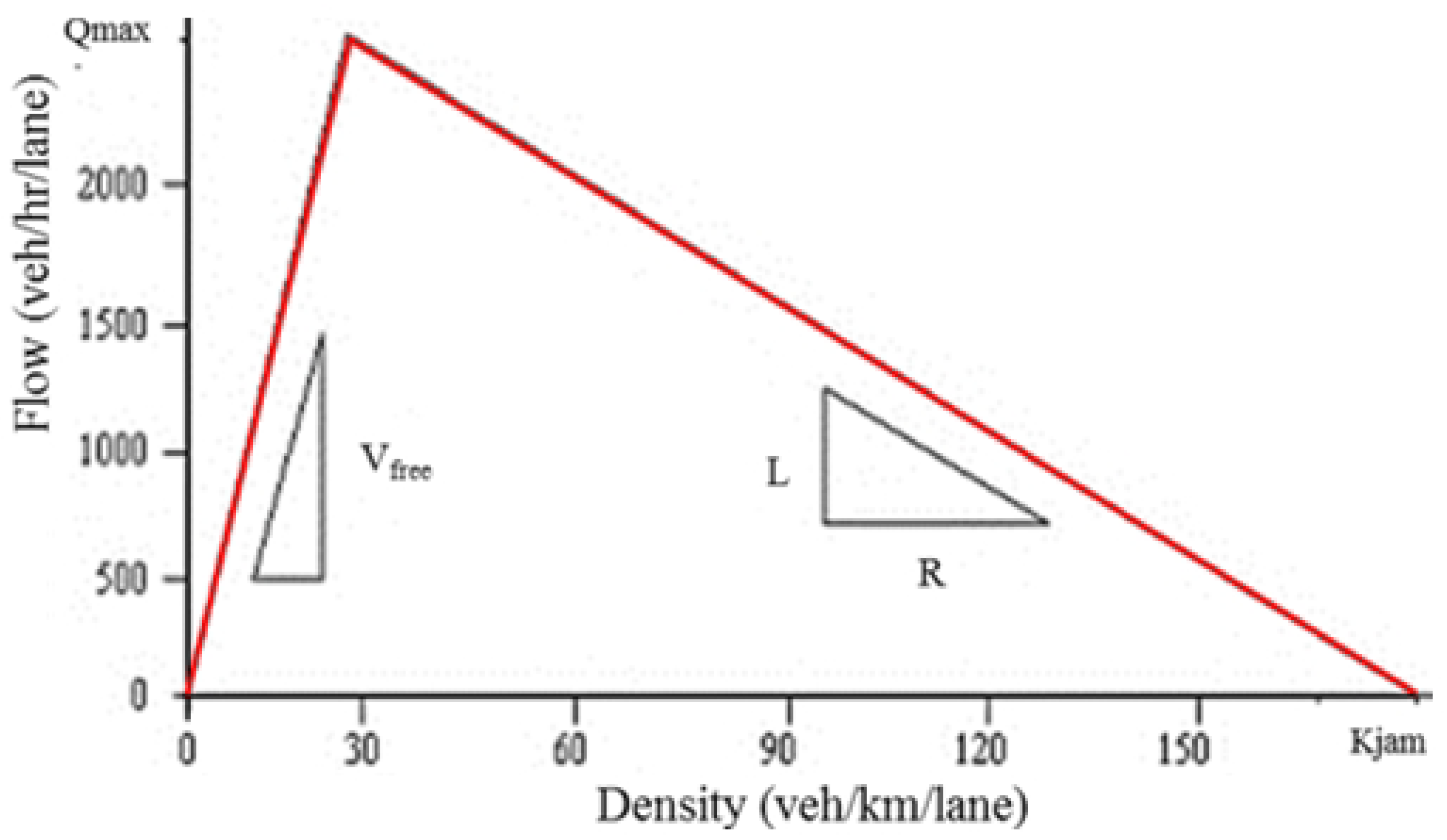
For the mesoscopic traffic model, a triangular diagram was chosen. This can be described by only three parameters, thereby minimizing the required input data. The triangular diagram is presented in Figure 6 below.

Values of the three macroscopic traffic-flow parameters for a specific vehicle type and a specific roadway can be determined from the free-flow speed of the link, the effective length (L), and response time (R) of the vehicle type, as shown in Equation (6) below.

$$Q_{\max }=\frac{1}{\left(R+\frac{L}{v_{free}}\right)},K_{jam}=\frac{1}{L},v_{wave}=\frac{L}{R}$$

(6)

where,

• $Q_{\max }$: maximal possible flow rate (veh/h/lane);
• $K_{jam}$: jam density (veh/hm/lane); and
• $v_{wave}$: speed (km/h) at which shock waves move through a platoon of traffic against the direction of flow, for a specific vehicle type.

VKT and VHT during the peak hour were selected as the two major performance measures. VKT is regarded to be a benchmark of network utilization, i.e., how much traffic can be served in the system. When demand increased, more vehicles traveled in the network and VKT increased; however, in the peak hour, this did not hold because VKT and VHT were determined by vehicles that had completed their trips. Due to network congestion, the number of exited vehicles (vehicles that had been served) stabilized when the system throughput reached capacity, while demand continued to increase.

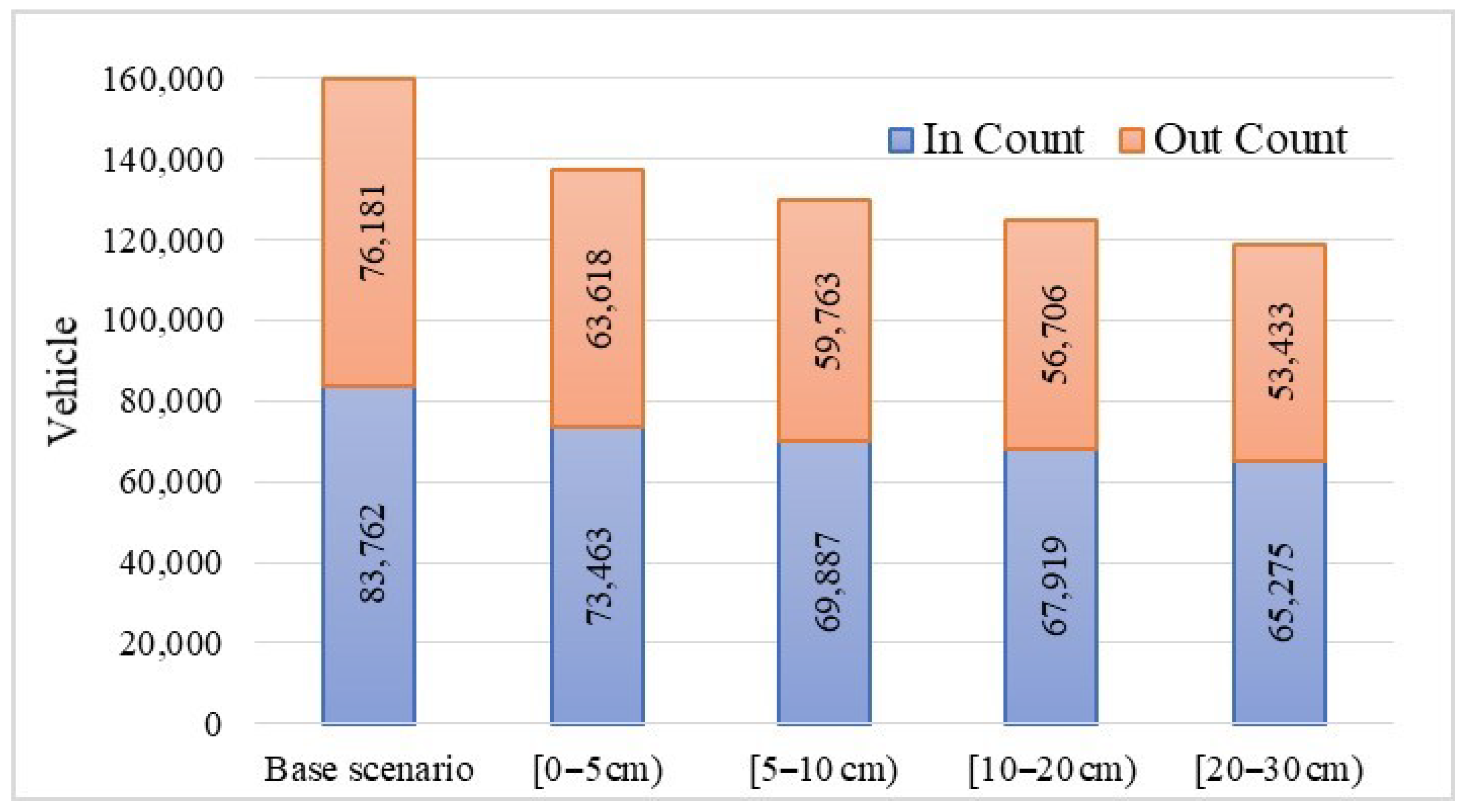
Figure 7 shows the number of vehicles entering and exiting from the network. The number of vehicle entries and exits in flooding scenarios shows a decrease from the baseline scenario to the high-depth scenario. This occurs because the number of trips by entering vehicles reduces, while for exiting vehicles, congestion in the network was high, and vehicle movement decreased. Most of the vehicles could not reach their destination on time.

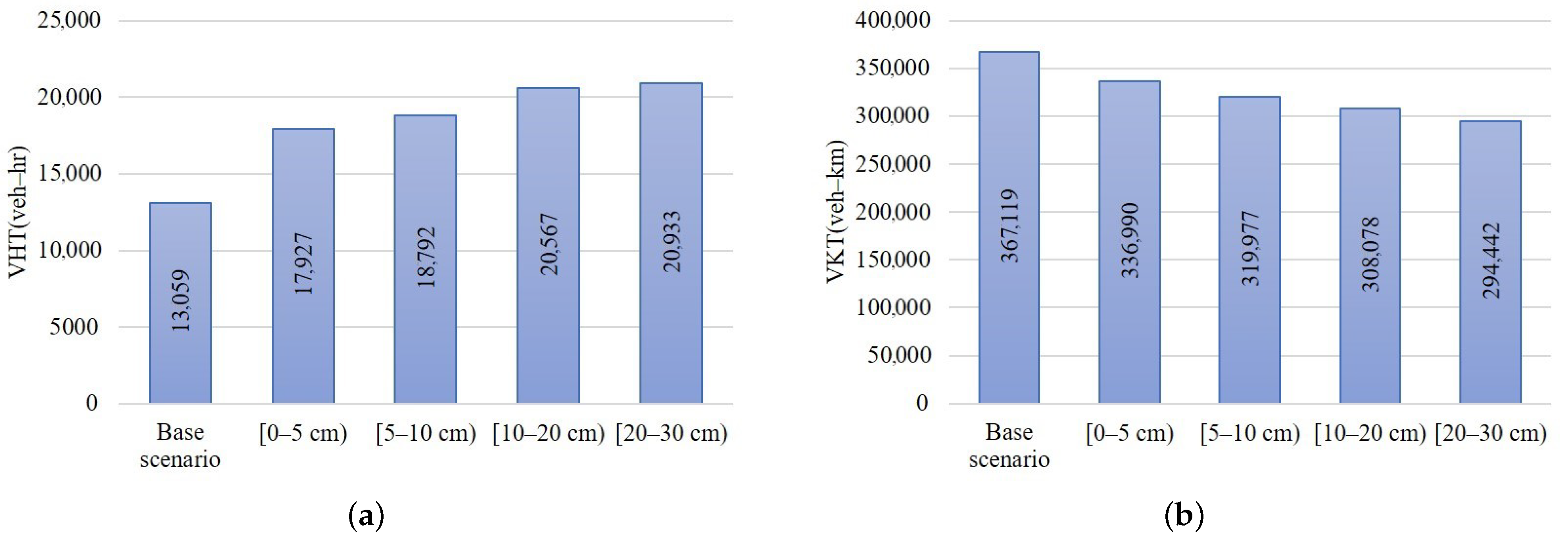
Figure 8 compares the base scenario (dry situation) and flood scenarios. The network indicator evaluation clearly explains that, when floods occur, VHT (Figure 8) increases, and VKT (Figure 8b) in the network decreases because the number of vehicles entering and exiting the network decreases.

5. Traffic Management during Flooding

The base dry scenario, and the highest flood of 20–30 cm scenario, both with and without traffic management measures, were simulated in the model. Results were compared to investigate the improvement of road-network performance after the implementation of traffic management measures for (1) an optimized signal system management, and (2) when traffic demand on arterial roads was induced onto the expressways. Road link performance in the study area was also evaluated.

5.1. Optimization of Signal System Management

The optimization of signal system management by synchronizing multiple signalized intersections generates a “green wave”, allowing for platooning vehicles to travel along the arterial road with minimal or no stops [28]. Synchronizing provides incentives for vehicles on arterial roads to speed and catch up with the platoon, so that they can pass through the intersection without any stops [29].

This study considered the mesoscopic model (Dynameq) that can model different intersection controls. Dynameq allows for signal offsets as inputs and provides improved computational efficiency compared to a microscopic model in a regional network. This is particularly important for simulation-based DTA. However, Dynameq has no program packet to cater for multiple coordinated intersections. Therefore, the microsimulation model (Vissim) was used to design a working layout for junction and traffic-signal design, and coordinate signal timings for Dynameq. The Dynameq model was used to evaluate how traffic was assigned to the local road network, considering delays as a result of flooding. Results of traffic flows and signal groups at each signalized node were input into the Vissim model to attain coordinated signal timings, which were then fed back into the Dynameq model to produce a final set of traffic flows for the network.

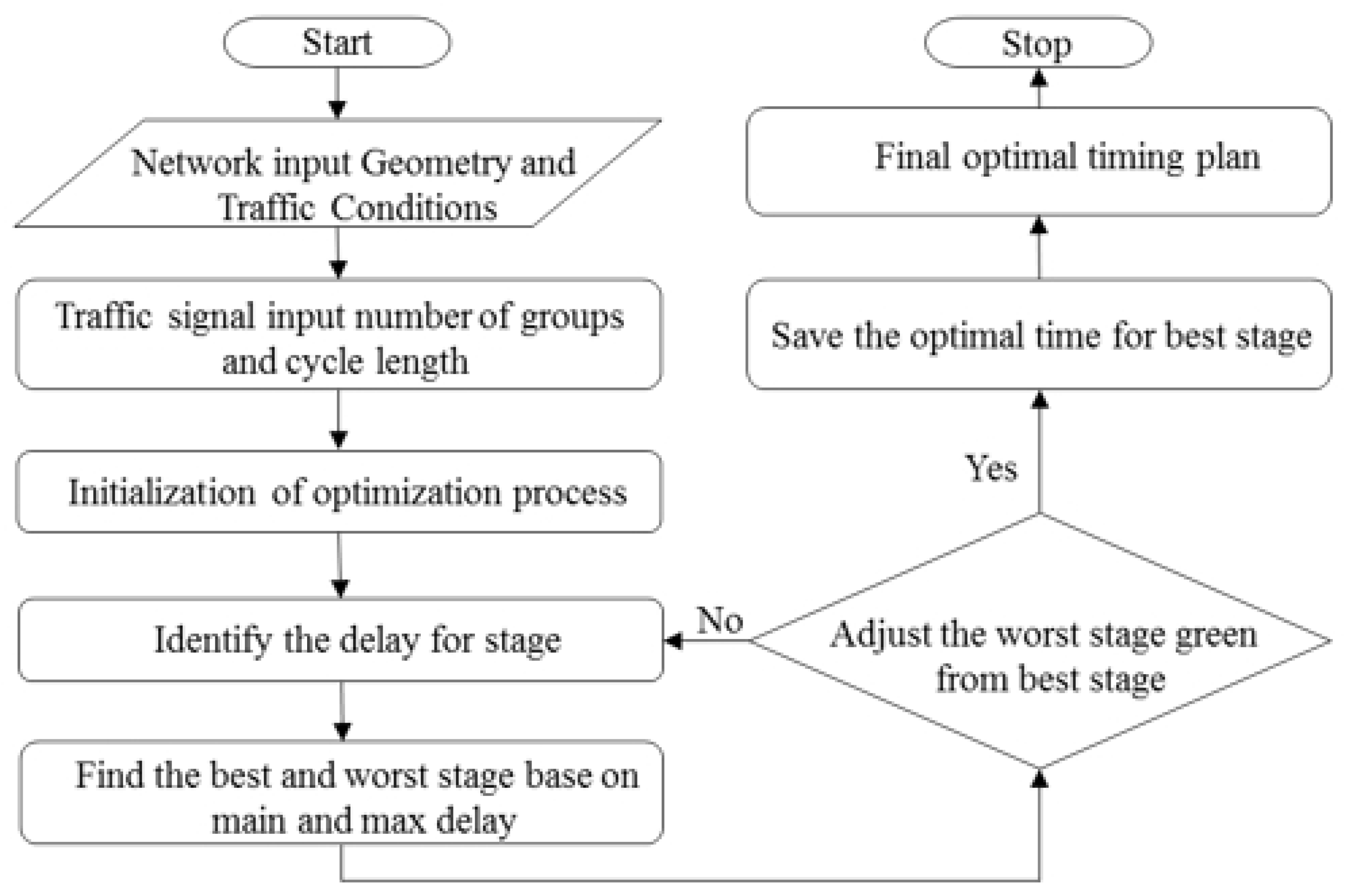
Figure 9 Vissim output using genetic algorithms for signal timing optimization for delay minimization [30,31]. Average delay of all vehicles passing through the signal heads at the intersection can be automatically determined from the node evaluation in Vissim. To optimize the signal stages, the highest delay times in all the stages were determined. Stages with minimal and maximal times were adopted as the best and worst stages. The worst stages’ green time was adjusted by deducting the time from the best stage. If the time could not be deducted from the best stage, the next best stage was selected for deduction. Similarly, the remaining stages were optimized for signal timing.

5.2. Use of Elevated Metropolitan Expressway with Free Tolls

The concept of an expressway with free tolls during flooding was suggested by [32] as an application of the MFD congestion pricing strategy (generalized cost) to improve mobility and relieve congestion in cities by reducing delays and the length of the rush hour. The DTA solution refers to assignments being in approximate equilibrium, where each driver attempts to minimize travel time or generalized cost, including intersection delays (total cycle time) and link cost as an operating cost including fuel cost and driving cost (value of time) multiplied by the time in the network to arrive at an operating cost. We added a perception penalty to the generalized cost for each road type, while the toll penalty was only used in scenarios that included congestion pricing. The toll penalty was calculated by dividing the toll cost assigned to a link by the assumed value of time to achieve a time cost in seconds of paying a toll. To be consistent with the dynamic model, the current model assumed that the value of time (fuel+distance cost, FC) was 86 s per km [27]. Trips were assigned to the network using the generalized cost (GC) Equation (7).

$$GC=P_{time}+LP+RP+Toll$$

(7)

where,

• $P_{time}$: generalized cost for movements;
• $LP$: left-turn penalty (10 s);
• $RP$: right-turn penalty (30 s);
• $FP$: facility penalty (fuel and distance cost);
• $Toll$: toll penalty.

Generalized cost in the expressway for this scenario is the same as another road type that provides a simplified description of travelers’ choices the effect of flood in their decisions to improve the city’s mobility. If the free toll is implemented during floods, road users are likely to take an elevated road instead of a road with the possibility of flooding. Therefore, the implementation of the free toll improves network performance and ensures the unobstructed flow of vehicles during floods.

5.3. Results of Traffic Management

The simulation period to evaluate how vehicles entered and exited the network during floods covered only peak hours. The numbers of vehicles entering and exiting, as shown by the model, were consistent for all scenarios.

Dry-scenario results in

Table 5. Result dry scenario.

		Traffic Management Measures
Performance Criteria	Scenario	(1)		(2)		(1 + 2)
		Value	Change %	Value	Change %	Value	Change %
In count (vehicle)	83,767	88,238	+5.34	83,638	−0.15	88,054	+5.10
Out count (vehicle)	76,181	81,466	+6.94	77,230	+1.38	80,542	+5.72
Waiting (vehicle)	77,529	158,333	+104.22	188,658	+143.34	166,236	+144.42
Travelling (vehicle)	61,552	168,006	+172.95	188,009	+205.45	172,573	+180.37
VHT (hour)	13,059	12,483	−4.41	14,354	+9.92	12,898	−1.23
VKT (kilometer)	367,119	431,079	+17.42	387,222	+5.48	419,080	+14.15

were assessed with traffic management measures. The elevated metropolitan expressway with free tolls (1) showed a slight change in the number of vehicles entering (in count) and exiting (out count) the road network by 5.34 and 6.94, respectively, but almost no change in optimizing the signals (2). However, the total number of vehicles in the network at the end of the interval (traveling) showed a high increase in all three measures. VHT increased in optimizing the signals (2) by 9.92%, as the in count was allocated to travel at intersections to minimize delays in the overall road network.

Table 6. Result of traffic management measures with flood scenario.

		Traffic Management Measures
Performance Criteria	Scenario	(1)		(2)		(1 + 2)
		Value	Change %	Value	Change %	Value	Change %
In count (vehicle)	65,275	68,862	+5.50	76,380	+17.01	81,333	+24.60
Out count (vehicle)	53,433	56,755	+6.22	65,612	+22.79	73,768	+38.06
Waiting (vehicle)	139,694	133,686	−4.30	91,242	−34.68	82,559	−40.90
Travelling (vehicle)	100,768	95,303	−5.42	85,720	−14.93	70,756	−29.78
VHT (hour)	20,934	19,538	−6.67	17,719	−15.36	15,209	−27.35
VKT (kilometer)	294,442	335,757	+14.03	343,741	+16.74	383,872	+30.37

shows the results of traffic management measures during flooding with the improved effectiveness of the flood depth of 20–30 cm scenario. Using the elevated metropolitan expressway with free tolls (1) showed a slight increase in the number of vehicles entering and exiting the road network, thus slightly improving VHT as vehicles chose alternative routes. By optimizing the signals (2), the number of vehicles exiting the network increased by 22% and improved VHT by a 15% reduction.

Overall, network efficiency in the dry scenario improved when traffic measures were taken, and there was only an increased VHT for optimization of the signal measures. In the flood scenario, the optimization of the signal condition showed better results than those of the use of the elevated metropolitan expressway with free tolls. Signal optimization impacted the overall network, whereas the use of the elevated metropolitan expressway with free tolls applied only to limited roads (expressway). When the elevated metropolitan expressway with free tolls and the optimization of the signal network were applied together (1 + 2), the number of vehicles exiting the network or completing trips increased by 38%, VHT decreased by 27%, and VKT increased by 30%. Overall, a substantial improvement in the network was achieved.

Results showed that VKT after applying traffic management measures by all vehicles showed improved performance of the whole network. VHT was reduced with a higher vehicle out count. The decrease in VHT indicated a better traffic situation. Similar to VHT, VKT is a meaningless criterion to reflect the change in traffic demand. Nevertheless, when combined with VHT, VKT indicated the extent to which drivers changed their route choices, and this affected network performance. Sometimes, other criteria such as average speed and delay are considered. However, evaluation results are mostly represented by travel time and travel distance.

6. Conclusions and Discussion

This study filled the research gap in three outstanding issues. First, previous work applied theaverage rainfall by using the whole area data. However, this study worked on a more specific area that considered the water depth on that road network. Second, using Bluetooth data in previous work provided the lack of transportation mode in upstream and downstream traffic, and outlier data can be cut from only abnormal speed, but probe data in this study can be represented as passenger cars and were updated every one minute. Lastly, previous work was performed as a traditional static model to evaluate the time effect from rise of rainfall. Therefore, this study used a dynamic model to solve the actual traffic problem.

(1)

MFD captures the relationships between average of flow and density characteristics, and plays an essential role in traffic-flow theory and transportation engineering. The MFD shape changed as a result of the network traffic operation under different flood levels. Varying degrees of impact induced the MFD shape change, and scatter occurred compared with in the dry conditions. Flood levels exceeding 30 cm had a greater effect on the discreteness of the MFD. The equation (in Table 1) presenting the relationships under different flooding depths indicated that the R-squared value reduced as flood depth increased, while continuity decreased. When assessing the MFD key parameters (in Table 2), an increase in flood conditions caused a reduction in free flow speed of −8.3%, −19.4%, −27.7%, and −30.5%, respectively, while the maximal flow of the network reduced by −28.3%, −38.1%, −42.1% and −49.6%, respectively, with density slightly reduced.

(2)

This study used a mesoscopic model that could simulate the movements of individual vehicles along roadway links using macroscopic traffic flow relations (free-flow speed, maximal flow, and jam density). These values were defined according to the remaining efficiency of the road network at each flood condition. Results offer a novel view of dynamic traffic conditions and provide rational scenario comparisons that are only possible with an equilibrium-based solution. Analysis of the impact of floods on traffic conditions used a calibrated mesoscopic traffic model as a baseline and introduced a flood scenario (20–30 cm). Tests on network indicators VKT and VHT were conducted to investigate the impact of perturbations of input parameters over the simulation results. VKT in the network decreased as flood depth increased because the number of vehicles entering and exiting the network decreased; thus, floods greatly impacted traffic behavior.

(3)

Two traffic management measures were selected to analyze their effects on network performance. The elevated metropolitan expressway with free tolls was appropriate to operate in a dry scenario because the generalized cost function used for path building was modified to reduce the perceived travel time on locals and collectors. In the flood scenario (20–30 cm), as in the present critical scenario, results indicated that theroad network performance of the whole network improved. Optimizing the signal control system improved network performance more than the expressway with free tolls in VHT and more than 2% in VKT did. However, combining the two measures for traffic management improved network performance by more than 27% in VHT and 30% in VKT compared to the critical scenario.