Article

Applying Spatial Analysis to Create Modern Rich Pictures for Grassland Health Analysis

by
Fabiellen C. Pereira
1,2,*,
Carol M. S. Smith
2,3,
Thomas M. R. Maxwell
1,2,
Stuart M. Charters
2,4,
Chris M. Logan
1,2,
Mitchell Donovan
5,
Sadeepa Jayathunga
6 and
Pablo Gregorini
1,2
1
Department of Agricultural Science, Faculty of Agriculture and Life Sciences, Lincoln University, Lincoln 7674, New Zealand
2
Centre of Excellence Designing Future Productive Landscapes, Lincoln University, Lincoln 7674, New Zealand
3
Department of Soil & Physical Sciences, Faculty of Agriculture and Life Sciences, Lincoln University, Lincoln 7674, New Zealand
4
School of Landscape Architecture, Faculty of Environment, Society and Design, Lincoln University, Lincoln 7674, New Zealand
5
AgResearch Limited Invermay Agricultural Centre, Puddle Alley, Private Bag 50014, Mosgiel 9053, New Zealand
6
Scion, 49 Sala Street, Private Bag 3020, Rotorua 3046, New Zealand
*
Author to whom correspondence should be addressed.
Sustainability 2021, 13(20), 11535; https://0-doi-org.brum.beds.ac.uk/10.3390/su132011535
Submission received: 27 August 2021 / Revised: 1 October 2021 / Accepted: 13 October 2021 / Published: 19 October 2021

Abstract

:
Grasslands are complex and heterogeneous ecosystems, and their health can be defined by the cumulative ability of their components to evolve, adapt, and maintain their integrity in the presence of stress/disturbance and provide ecosystem services. Herein, a design approach is used to generate alternative and multifunctional pastoral livestock production systems that enhance grassland health. As a way of understanding the complexity of grasslands and initiating the design process using systems thinking, rich pictures emerge as a useful method. As rich pictures are subjective views, geographic information systems (GIS) could be applied to improve the veracity of their outcomes, as both techniques are forms of an analytical process. This paper reports the application of GIS to a case study of a high-country farm to generate and combine different thematic maps to create a modern rich picture. The rich picture is a combination of remote sensing data (altitude, slope, aspects, and the Normalized Difference Vegetation Index (NDVI)), and on-the-ground data (plant species distribution and diversity and soil chemical, biological, and physical parameters). Layers were combined using a multi-criteria evaluation (MCE) based on the analytical hierarchy process (AHP) to create a final rich picture. The results highlight dissimilarities in perceptions of what underpins ‘grassland health’ between researchers in different fields and with different perspectives. The use of GIS produced a modern rich picture that enhanced the understanding of grassland health and allowed for the identification of gaps, values, and possibilities for future research work.

1. Introduction

Pastoral livestock production systems are facing adjustment requirements to evolve continually as adaptive systems and ensure the sustainability of grazing ecosystems. These requirements are based primarily on food production, but also include the need for responding to growing public concerns regarding their negative environmental footprint (degradation of natural resources, greenhouse gas emissions, biodiversity loss, etc.) that affects the provision of grassland ecosystem services and, in turn, threatens the stability of farming systems. This context calls for the introduction of new practices in farming systems and the use of design techniques to create alternative and more sustainable pastoral livestock production systems that can attend to multiple and pre-defined demands [1,2,3].
A design approach for creating alternative and multipurpose farming systems is well suited as it uses current knowledge and/or creates new knowledge [3] to generate means, methods, and products [4] that will be put in action to transform a specific situation [5] and attain specific predefined goals [4]. An explorative approach is essential in this process as a starting point to analyze the current situation of a system, identify gaps within it, and apply available knowledge to set goals and evaluate possible alternatives to meet them while still considering the constraints of available resources [3,6].
Pastoral livestock production systems are placed within grassland ecosystems, involving natural environments, social networks, cultural features, and multiple areas of expertise (e.g., geography, agronomy, animal physiology, and agroecology). Grasslands are heterogeneous environments in which temporal and spatial scale plays an important role in landscape patterns and ecosystem processes [7]. Heterogeneity in this context is referred mainly to the variability in vegetation structure, composition, density, and biomass across the space [7], with each vegetation type having different growth patterns and responding to environmental factors in different ways, and thus diversely affecting the system and making it complex and dynamic. The understanding of how those systems behave and their nature is paramount to create alternative and multifunctional systems, as their dynamism and complexity mean that any intervention may lead to uncertain outcomes and unpredictable collateral effects that are not always desired [8]. As an example, the increased productivity of a farm due to the inclusion of a new crop variety may be followed by a decline in yield due to pests and disease incidence [9], or increased global temperature due to greenhouse gas emissions resulting from the intensification of livestock; this is also a factor that can cause pollinator populations to decline, in addition to pesticide use and habitat loss [10], as well as its unknown effects on pasture availability and composition from increased stock density. Therefore, a more integrative and systematic perspective in this explorative process towards the agricultural context is required to uncover the multiple services and purposes that grassland landscapes are capable of offering [11].
Systems thinking theory fundamentals could facilitate comprehension of the complexity and dynamism of pastoral livestock production systems by providing an overview of their components, associations, and processes [12], thus contributing to the explorative approach in the design of alternative and multifunctional systems. As a systems thinking tool, rich pictures would trigger the analytical visualization of the current situation of pastoral livestock production systems. Rich pictures attempt to capture everything to be perceived as a part of the case, including interconnections, subjective elements, and non-linear structures [13]. Rich pictures facilitate research translation by improving the timeliness and relevance of research questions [14], and they could therefore help in the framework construction for designing alternative pastoral livestock production systems by depicting potential issues that designers should focus on and the potential implications of any action taken.
Rich pictures are usually drawn by several hands with no formal rules to raise debates within a group of people, and they represent different points of view from stakeholders’ perspectives [15]. They are a free-form type of diagrammatic representation used as a facilitating tool in an analytical situation [16]. However, rich pictures are soft modelling tools from soft systems methodology, which means that they do not concretely represent external reality but instead personal views [14,17]. As a way of enhancing a rich picture, we propose the use of technology and spatial data analysis to create a more realistic rich picture. This approach would consolidate and better represent the components and outcomes of management and ecosystem processes occurring within pastoral livestock production systems that handmade drawings, otherwise, could not measure or capture.
Technology and spatial data analysis bring precision into farming systems [18]. As an example, geographic information systems (GIS) have been an important technological tool in landscape visualization by creating virtual ‘pictures’ with mapped information and simulating reality under a particular set of assumptions [19,20]. Some advantages of GIS are the integration and interactive visualization of different spatial data layers created from various spatial analysis techniques for the decision-making process [19], such as identifying suitable areas for specific plant species growth [21], susceptibility of specific spatial occurrences (landslides susceptibility, [22]), and suitability for land use [23]. Although assumptions should be made by experts for the creation and integration of layers, the decision-making process is based on the final map. The addition of the rich picture concept would enhance experts’ participation, discussion, and decision making during the process of creating the maps, potentially affecting the final product.
Using GIS to create a rich picture could advance understanding of how grassland components and their features are related and how this interaction characterizes pastoral livestock production systems, facilitating the explorative approach in the design process. Therefore, this paper reports the application of spatial analysis (GIS) to a high-country farm to generate and combine different thematic maps to create a novel and modern, rich picture as a starting diagnostic in a design process for enhanced grassland health.

1.1. Background

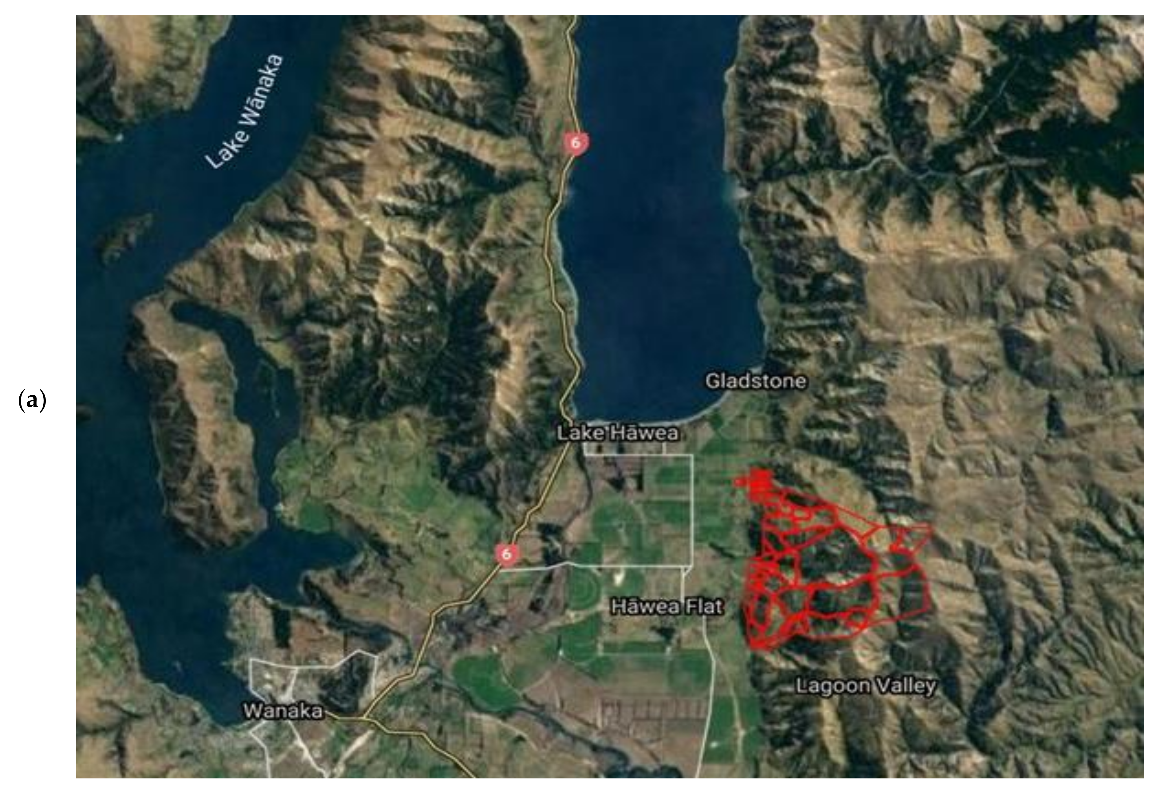
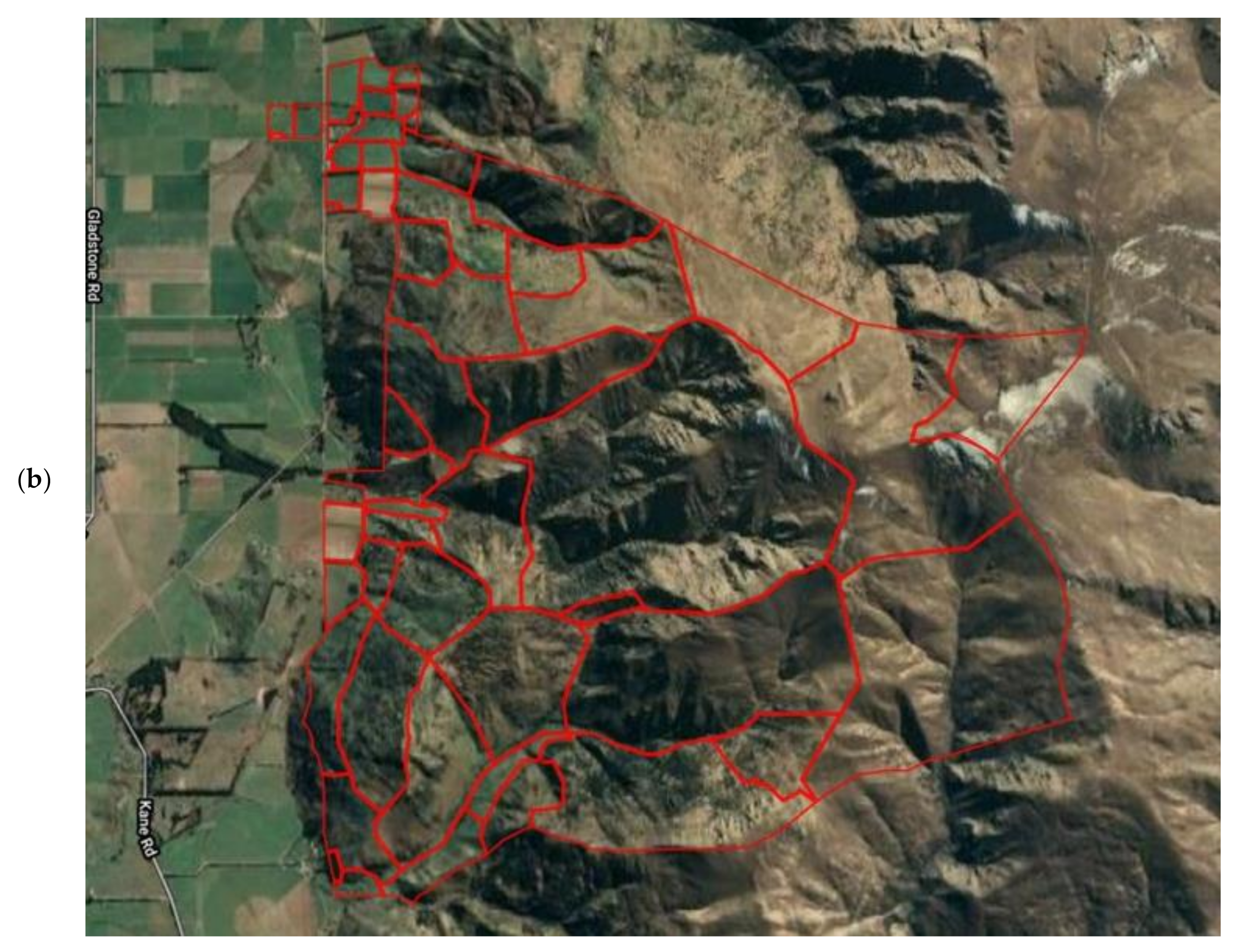
1.1.1. Designing Future Productive Landscapes and the Case Study of Lincoln University’s Mount Grand Station

The case study for this research is the Lincoln University high-country farm of Mount Grand Station (LUMGS). The station is located on the eastern wall of the upper Clutha valley in the Lindis ecological district of the South Island, New Zealand (NZ) (See Figure 1). The total area of the station is 2131 ha, of which 1602 ha is used as a pastoral system, while the remainder is a conservation area. Around 7% of the area is flat, while the remainder is steep hill country. The annual rainfall average is 703 mm and the annual mean temperature is 10.6 °C (17.25 °C in summer and 2.25 °C in winter) [24,25].
The farm contains around 3000 Merino sheep, which are split into small groups distributed across the total area at different times of the year, according to seasonality. Groups vary between 50 and 650 animals depending on the paddock area. Most of the paddocks used are in low- to middle-altitude areas (<900 m) while some upper paddocks (<1100 m) have not been used in the last four years. The grazing time in each paddock depends on pasture availability, weather conditions, and the productivity stage of animals (e.g., lambing, weaning), and varies between two and five months.
The station is a case study for a design project from the Centre of Excellence in Designing Future Productive Landscapes at Lincoln University. The design approach implies the construction of a framework, where strategies, methods, and kernel theories are used to achieve a known goal [4]. Therefore, this requires a clear definition of grassland health and how to assess it in order to meet the goal of enhancing it.

1.1.2. Grassland Health

We have defined grassland health as the ability of soils, microorganisms, flora, and fauna (including humans and grazing animals) present in the system to evolve, adapt, and maintain their integrity in the presence of natural or human-caused stress/disturbance and provide essential components to sustain ecosystems. Grassland ecosystems provide ecosystem services, which are all the ecosystem functions and products that benefit and meet the needs of human survival, life, and well-being, including soil protection from erosion [20], the provision of food and water, pollination, regulation of climate, water and air, primary production, nutrient cycling, and aesthetic/cultural values [26,27,28]. These services vary between different physical environments, grassland types, and their degree of intactness and adaptation in response to biogeographic events and cultural–historical evolutive processes over time and space [29,30]. In the LUMGS context, the understanding of its physical features and its current vegetation community pattern and structure as a consequence of its evolutionary process is, therefore, paramount to defining and assessing its grassland health.
With a clear and defined objective, an explorative analysis to evaluate the current context and set a plan of actions is the starting point in the design process. Accordingly, the current grassland health and condition of LUMGS should be assessed. As grasslands are complex environments, as seen by our complex and holistic definition, to establish an assessment of its health, we applied a systems thinking theory as a holistic approach to enhance our understanding of how components and processes within temperate grasslands interact and define the health condition of LUMGS.

1.1.3. Rich Pictures and GIS

Rich pictures, as systems thinking tools, are ideal for identifying opportunities for change to occur, as they work as an analytical method that aims at capturing as much information as possible to enhance the understanding of complex/messy situations [17,31]. By recognizing the processes underway, rich pictures help in the identification of priorities, current and potential issues, and future actions towards a specific context [32]. The outcome of rich pictures, therefore, signals further approaches and research tools and directs possible improvements [17,31]. As an alternative to rich pictures, GIS, an analytical method, has been contributing to farming systems with decision-making support capabilities by providing valuable information through the creation of virtual maps and insights about a particular environment [19]. Furthermore, the use of GIS has been reported to address cultural and traditional values and concepts [21] and embed community participation [33], as in rich pictures.
Rich pictures are a structureless and rule-less way of communication that produce multi-perspective representations and models of complex systems [32], while GIS produces virtual pictures [19] that allow for the assessment and critical evaluation of landscapes [34]. Therefore, as we seek an enhanced understanding of complex environments to initialize the design process, we applied GIS for the creation of our rich picture. The use of GIS is aimed at adding realistic information for the components and design process of LUMGS to enrich the informative value of the rich picture, thus facilitating the explorative analysis. As both rich picture and GIS require a methodology accounting for different perspectives and concepts, we used multi-criteria evaluation (MCE) to combine the different virtual maps and contemplate the community participation principles of handmade rich pictures. The next section will describe how the rich picture was created (Figure 2).

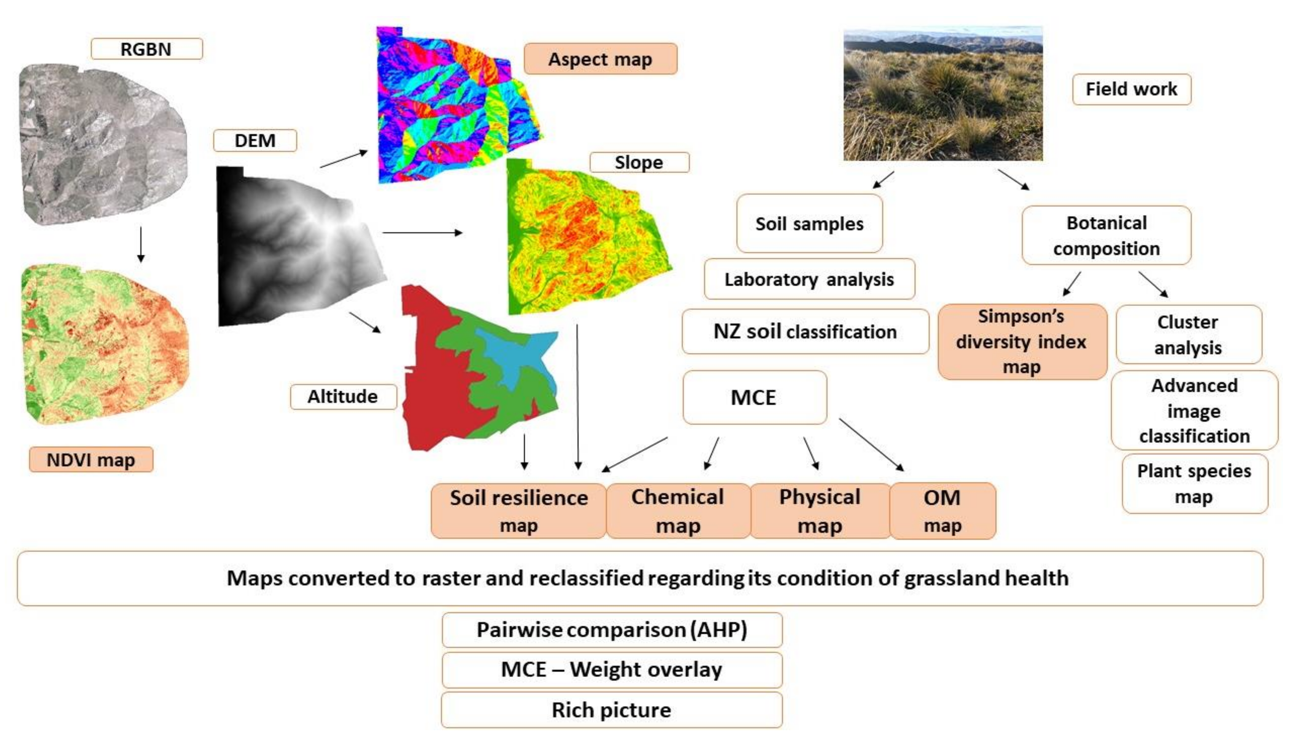
2. Materials and Methods
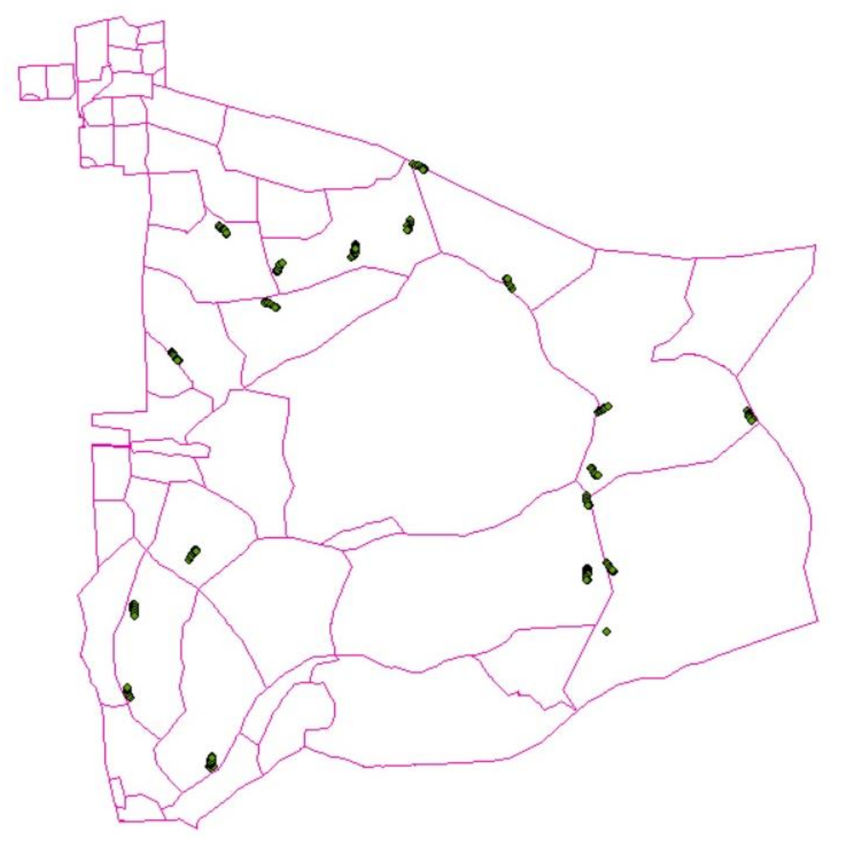
2.1. Rich Picture

The rich picture was built through a combination of remote sensing data and on-the-ground data with ArcGIS/Arcmap 10.7.1® software depicting vegetation and soil characteristics as a means of indicating the health condition of vegetation and topographic features at LUMGS based on our previous holistic definition about grasslands health. A high-resolution base dataset of LUMGS was captured (flying at 1550 m) for Summer 2020 in terms of RGBN 16 bit (Red, Green, Blue, NIR) multispectral imagery at 12.5 cm of ground sampling distance and light detection and ranging (LIDAR) to generate digital elevation models (DEM) and digital terrain models (DTM). A DEM is a representation of the topographic surface, and a DTM augments a DEM by including vector features of the natural terrain [35].
The DEM/DTM were used to generate topographic layers, providing altitude, slope, and aspects, and the RGBN image was used for the Normalized Difference Vegetation Index (NDVI) of the area. Slope and NDVI have already been used as remote sensing assessment tools of grassland health in other studies, with slope as a limiting factor on ecosystem resilience and NDVI as an ecosystem vigor indicator [36,37]. Vigor is an ecological indicator of primary ecosystem productivity over time and space [38], used to assess grassland health [39], and it can be assessed through NDVI as it represents the amount of green vegetation in an ecosystem [38]. The NDVI (Equation (1)) is generated from measurements of spectral reflectance obtained in the visible red band and the near-infrared band [34].
NDVI = NIR RED NIR + RED
Aspect indicates the orientation of a slope to the sun, therefore suggesting the level of incident sunlight radiation on it, while altitude is a highly influential topographic attribute on the abiotic factors of an environment [40]. Aspects and altitude determine the microclimate of an area, and thus play an important role in vegetation patterns of productivity, species composition and biodiversity [41,42,43], and soil chemical, physical, and biological parameters [44,45,46], all of which are essential attributes used to assess grassland health, especially in a highly heterogeneous environment such as LUMGS.

2.1.1. Botanical Composition

On-the-ground data collection during summer (December 2020 and January 2021) to detail the botanical composition, vegetative cover, and soil condition of hill country grassland areas was conducted to validate vegetation and soil historical data of LUMGS, based on the literature provided by Duncan et al. (1997). Data sampling occurred in areas classified as ‘hill country low-producing grassland’ according to the new vegetation classification map of LUMGS created by the Centre of Excellence (unpublished data). Other vegetation areas of LUMGS also include grassland ecosystem components (such as shrubs, exotic forest, high producing grassland, Kanuka), but because they were dominated by other kinds of vegetation (specific shrubs or trees), they were categorized differently. The decision for taking samples only in the areas classified as ‘hill country low-producing grassland’ was taken to ease and reduce the amount of field work, due to time and financial limitations. These areas were subdivided into three categories: high altitude (>1100 m), mid-altitude (900–1100 m), and low altitude (<900 m). Sample points were collected from each of the three categories (Figure 3).
Aspects of the area were also considered and registered in every sampling point, in which we classified three categories: Sunny aspect—considering north, northeast, and northwest face; moderate sunny aspect—considering west and east faces; and shady aspect—considering south, southeast, and southwest hillside faces. Transects of 100 m were randomly positioned six times in each category of altitude, and five (1 × 1 m) quadrats equally distributed over each transect were visually evaluated to register the absolute cover percentage of species present in each quadrat. The cover percentage was then used to calculate the absolute frequency, relative frequency, and value of abundance index of species according to Ellenberg and Mueller-Dombois (1974 [47]). Furthermore, Simpson’s diversity index [48] was calculated as:
D = 1   n n 1 N N 1
where n is the number of individuals from the same species and N is the total number of all individuals. Both indices were calculated for each altitude considered for sampling.
The botanical composition resulted in more than 40 different species, including grasses, legumes, herbs, and shrubs. However, we listed only species that had an importance value that considers relative frequency and cover higher than five (Table 1). Some species were found at all altitudes, but with different importance values, indicating different abundance or frequency. Most of the species were also reported by Duncan et al., (1997), the database used to design the methodology of the current study.
The Simpson’s diversity index was calculated as 0.91, 0.89, and 0.88 for low, mid, and high altitudes, respectively. A higher value (closer to one) of Simpson’s diversity index indicates a more taxonomically diverse environment. Landscape diversity and richness and vegetation coverage are indicators of the level of organization of an ecosystem [36], an important ecological indicator of grassland health that is related to the biodiversity of components and their interactions [38,39]. The diversity of plants is also positively associated with increased biomass production, which is an important ecosystem function in grasslands and a parameter that indicates vigor, besides triggering biotic processes that promote multifunctionality and assure better integrity, stability, and resilience of ecosystems [49,50,51]. Therefore, the diversity index is a good indicator of grassland health condition, and our range suggests high diversity in all altitudes, being an essential parameter to be considered in our explorative analysis.
Sampling points were georeferenced with a GPS (GPSMAP 76S Garmin, 3 m) and imported to ArcGIS/Arcmap 10.7.1® software. Botanical data were submitted to a principal coordinate analysis developed for the matrix of species cover composition using the Bray–Curtis method to understand the degree of similarity between the unit samples (quadrats) regarding the cover composition of species. The average linkage method was used for the hierarchical cluster analysis using the vegan package [52] on R software version 3.4.0 [53].
The cluster analysis (Figure 4) resulted in four groups of unit samples (quadrats) that presented similarities, and each group was represented by significant species; these are different from the ones selected with importance values higher than five.
The cluster analysis resulted in a low sum of axis, which was not desirable. However, we aimed to use this methodology to propose new tools to illustrate the distribution of the most abundant plants in LUMGS, and we acknowledge that this methodology should be improved in future works. Alternatively, other types of cluster analysis could have been performed, or a higher number of samplings could increase the accuracy of the analysis. However, as we were satisfied with the groups that resulted from the analysis, we used the results to demonstrate and propose the methodology and provide us with an idea of plant distribution in LUMGS.
Based on this result and the results from the value of abundance index of species, advanced image classification methods (machine learning and object/pixel-based classification) from Arcmap were used to create a map depicting the most abundant plant species and its distribution across the classes of low-producing grassland of LUMGS. Significant species from cluster analysis results were drawn as polygons over pixels values of the RGBN image to create a training dataset (signature file). The training dataset was used to train a machine learning model in the support vector machine learning and apply it to recognize patterns in the area in terms of species distribution. The support vector machine learning tool is a supervised learning method based on statistical learning theory [54]. The classify raster tool was used to extrapolate this information over the whole area. The map was created based on fieldwork and pixel-based classification in Arcmap. Ground proof was not attained due to the small size of quadrats and GPS accuracy, but the distribution of species across the area corresponded to the results of botanical composition performed on the ground, regarding species abundancy in each altitude according to Duncan et al. (1997).

2.1.2. Soil Analysis

Soil is a key component in grasslands and plays a vital role in ecosystem processes, influencing its vigor, organization, and resilience, the three ecological indicators that determine grassland health [36]. Vigor and organization were previously defined, whereas resilience is the system capacity in maintaining its structure and function in the presence of stress [38,39]. Soil resilience definition follows the same concept and is related to the term sustainability due to its multifunction [55].
The influence of soil on ecological indicators depends on the ability of its single properties and its process to interact and perform soil functions, therefore determining its health [56,57]. Several attributes/indicators have been used to assess soil health. Bearing in mind that soil has chemical, physical, and biological components, we have selected soil indicators carefully covering those three areas to represent its health [57].
Soil samples were taken from the same areas and sample points as vegetation composition evaluation. For chemical and biological attributes, samples were taken by using a quick test auger to sample 0–10 cm depth, which were analyzed at Lincoln University. Subsamples were broken up, air-dried, and ground to pass through a 2 mm sieve for further soil analysis.
The moisture content of air-dried samples was determined gravimetrically by drying at 105 °C for 8–24 h. A moisture factor was applied in calculations of the results to convert air-dried results to an over-dry basis. Soil pH and electrical conductivity were determined in a 1:2.5 soil:solution ratio according to the procedure developed by NZ Soil Bureau for NZ soils [58].
The organic C and total N of soil were measured by using an Elementar Vario-Max CN Elemental Analyzer. Soil samples were combusted at 900 °C in an oxygen atmosphere and any elemental carbon and nitrogen were converted into CO2, N2, and NOx. NOx was subsequently reduced to N2. These gases were then passed through a thermal conductivity (TC) cell to determine CO2 and N2. The Olsen P method was used to determine soil phosphorus (P) fertility on a 0.5 M NaHCO3 (pH 8.5) extraction using a spectrophotometer [58,59].
A simple single-extraction procedure with ammonium acetate solution was used to measure exchangeable cations in soil (Ca, Mg, K and Na). Soil sulphate sulfur (S) and extractable organic sulfur on soil surfaces were measured by extraction with potassium phosphate (KH2PO4) solution from fresh soil samples [60]. Soil particles’ size distribution was manually calculated for the determination of soil texture. The stability of an aggregate test was not conducted, as samples presented a lack of structure and no aggregates; therefore, the analysis was unfeasible.
Aluminum cores (99 mm internal diameter and 75 mm high) were used to collect soil samples for determining physical parameters of field capacity, microporosity, and bulk density. Undisturbed soil cores were saturated and equilibrated at −10 kPa on tension tables and results were calculated from oven-dry weights.
Statistical analyses for soil results were performed in R [53] using R package lme4 [61]. Multiple linear regression was used to analyze the effect of different altitudes and aspects on soil parameters (pH, N, K, extractable organic S, electric conductivity, C/N ratio, Ca, moisture, exchangeable cations, C, P, S, Mg, field capacity, bulk density, porosity, macroporosity, volumetric water content, and water-filled pore space). Model assumptions were adjusted graphically for normal distribution and homoscedasticity of the residuals. P values were obtained by Wald X2 test type II (p < 0.05 or p < 0.01). Volumetric water content and water-filled pore space were submitted to the Kruskal test, a non-parametric test, as the data did not show a normal distribution even after logarithmic or square root transformation.
Regardless of whether soil parameters were affected by altitude or aspect, the chemical results (pH, N, K, extractable organic S, electric conductivity, C/N, Ca, exchangeable cations, C, P, and Mg) were contrasted with value ranges for NZ soil [58] to create the layers for the rich picture, and most of the parameters were framed in the same classification (Table 2). The remaining parameters were compared with the literature values.
Considering that soil parameters affect soil health collectively, and that evaluating them as individual factors would lead to a flawed conclusion about the health condition of a complex system, parameters were integrated by using MCE to produce four soil maps: a resilience map (slope, erosion susceptibility, altitude, pH, C, P, electric conductivity, and exchangeable cations), a chemical map (extractable organic S, C/N, N, exchangeable cations, Ca, Mg, K, Na), a physical map (bulk density, field capacity, porosity, macroporosity, volumetric water content, and water-filled pore space), and a map that depicted organic matter content. The categorization of the parameters into the maps was defined by the authors. Maps were created by classifying polygons, drawn at each altitude, according to the classification of each parameter.

2.1.3. Multi-Criteria Evaluation

Each map layer (soil layers, topographic layers—aspects and NDVI, and diversity index layer) was converted to a raster layer in Arcmap and classified, using reclassify tool, into one of three grassland health condition categories for sustained pastoral livestock production systems (low, moderate, or adequate condition to sustain pastoral livestock production systems, Figure 5). The categories were a range of values attributed to each of the parameters defined along with three workshops covering 15 researchers/experts on soil, vegetation/biodiversity, production systems, and existing systems. Then, an MCE was performed, using a weight overlay tool, to combine GIS layers using weightings derived from pairwise comparison matrices performed by a group of six experts from the research group, following the analytical hierarchy process (AHP) described by Saaty (1980 [62]).
We applied MCE to hierarchically combine criteria/attributes (each layer) based on each individual perspectives. We used this approach as traditional rich pictures are free-hand drawings made by a group of people with a goal in mind that aims at depicting their perspectives concerning a specific context. The group of six people was small and purposefully selected as the creation of rich pictures is agreed to work better in the context of a small number of people [14,15]. Moreover, the group must be aware of the theme to be investigated in order to determine its constituents [63]. Therefore, this process was run with an overall goal in mind—assessing the current health condition of LUMGS grassland, in which attributes were weighted for importance before combination according to individual knowledge of each expert (see a similar process in [21,34]). The MCE yielded a single hierarchically overlaid map representing grouped criteria to satisfy the goal according to experts’ perspectives. The map was then converted to a browser-run 3D map in ArcScene, thus creating a 3D rich picture of LUMGS illustrating areas as having low—pink color, or moderate health condition—green color. (Video S1: 3D rich picture of LUMGS).
As soft modelling tools, there are not definite or unique problem definitions in rich pictures but instead personal perspectives [17]. A rich picture is a physical drawing that encourages debate and offers shared thinking to improve people’s understanding from their different perspectives towards a complex context [32]. Therefore, rich pictures are not supposed to be validated but judged by their creators regarding whether they meet the goal behind their creation, which is the reason why the group of people should be small, and purpose selected [14,15]. To attend to the principles of a traditional rich picture, the final rich picture was evaluated by the same group of people that created it, as a means to ensure those goals were satisfied. Rich pictures are a product of discussion within groups in workshops or meetings. Therefore, the MCE was performed more than once, creating different ranks and different rich pictures. After each outcome from the AHP and MCE, meetings were taken to evaluate the importance of each layer for assessing grassland health and the value (factor of influence) attributed to it. This exercise raised discussions about the definition of grassland health, which was reviewed several times, and about the attributes that led the group to redo the pairwise comparison, bearing in mind the previous discussions. Ultimately, the final rich picture is the result that better satisfied the goal of assessing the current health condition of LUMGS based on the group of experts who created it.

3. Results

Results from soil particle size distribution characterized the soil texture of LUMGS as silt loam. Although this parameter was not inputted to the rich picture, it contributes to understanding the condition of soil and vegetation in the area, as it affects many of the chemical and physical parameters of soils [64]; including susceptibility to erosion and ability to support a vegetation community, and the abundance and variety of plants [65]. The same is true of soil classification, (Figure 6), which is predominantly composed of brown (upland slopes) and Pallic (loess parent material) soils [66], according to Hewitt (1998 [67]). Brown soils, according to Landcare Research [66], cover a great extent of NZ soils and occur in places where summer drought is not common and that are not waterlogged in winter. They are relatively stable with good biological activity but have low to moderate base saturation. Pallic soils, on another hand, do not cover a large part of NZ soils and occur in dry parts of the country. They are susceptible to erosion, have medium to high nutrient content and base saturation, but a low concentration of organic matter. Pallic soils tend to be more compact and require more land management attention from farmers, especially during wet conditions, while brown soils are better structured and are more resistant to treading damage [20,68]. Knowledge of soil classification and soil type is essential to understand the results of the analysis performed in this study, so as to relate it with vegetation tendencies. Having this information not only contributes to explaining the current situation of LUMGS but also provides a direction for possible actions to be taken for the enhancement of grassland health under livestock production systems.
The influence of altitude and aspect features on soil parameters is shown in Table 3. Altitude was a factor of influence for most of the chemical parameters, while aspect was only significant for pH, soil moisture, and C/N ratio, where interaction with altitude was observed. At high altitude, pH was similar for all the aspects and mid-altitude—shady aspect and low altitude—sunny aspect (5.02). At low altitude, moderate sunny and shady aspects, and mid-altitude—sunny and moderate sunny aspects, pH was 5.32. Moisture content was lower at low altitude regardless of aspect (22.42%), it was higher for mid- and high altitude, for shady aspect in mid-altitude, and for moderate sunny aspect (43.08%), with intermediate values at high altitude, moderate sunny and sunny aspects, and mid-altitude, sunny aspect (31.06%). The ratio of C/N at high altitude was the same for all aspects and mid-altitude moderate sunny and shady aspects (14.65). This ratio was lower for the sunny aspect at mid-altitude (13.08) and even lower for all aspects at low altitude (10.86).
Although some parameters were different according to altitude or aspect, soil layers were created based on the range of values for each altitude according to NZ soil classification and the literature, as previously stated.
The distribution of plant species at LUMGS is illustrated in Figure 7. This map was not included in the creation of the rich picture per se but adds valuable information to the rich picture outcome and the design process.
The pairwise comparison result with the weights for each criterion/attribute is shown in Table 4. According to the combined individual perspectives from six experts, soil resilience is the most influential criterion for assessing grasslands health, while the least influential criterion is physical parameters of soil.
The relative importance of each criterion for defining and assessing grassland health, according to the MCE results, derived a map characterizing the grassland condition of LUMGS as a low or moderate health condition (Figure 8). The map suggests that most of the area (97.7%) is considered as having a moderate health condition of grasslands, with a small proportion (2.3%) of the area being considered as having low or no area considered to be in good health.

4. Discussion

These results are dependent upon the weight of influence of each criterion/layer inputted to the creation of the map, and how each criterion/layer (either as a result of spatial analysis or fieldwork) is categorized in a grassland health condition range. The categories were defined by consulting experts and the literature, while the relative importance of each criterion was decided by the group of six people. During the process, individual layers were discussed and modified until an agreement within the group was achieved. As more discussion and participatory involvement occurred, the perspectives towards the rich picture became more critical, and different perspectives provided different influences for different parameters, thus producing different maps. This is the ultimate reason why rich pictures should be made by a group of people with different perspectives, as an attempt at capturing and representing a context viewed by different points is vital.
Based on this, the result of evaluating the grassland health condition of LUMGS is mainly a consequence of the topographic context of the station (slope, elevation, aspect), which has a high influence on vegetation and soil parameters. Besides this, the grazing management on the station has a great impact on soil–plant interactions, with further consequences for grassland health. However, grazing management effects will not be discussed in this work. The rich picture is the starting point for a design project that aims to enhance grassland health and indicates the current condition of LUMGS for the planning of further actions that will consider grazing management.
Our rich picture compiles soil, topographic, and vegetation parameters, which are key components of grasslands that further affect ecosystem processes. Understanding their interaction on ecosystem services contributes to defining grassland health. However, uncertainties and gaps caused by data availability constraints must be acknowledged.
We are aware that, given the previous definition of grasslands health, some parameters are missing. As a complex system, components and processes are related, so available information used in this work can indicate and provide insights about other components and processes that take place in grasslands that define their health. However, measurements that assess and inform other grassland components and processes, such as microorganisms and fauna, were not collected. We strongly suggest the addition of these measurements in future work to achieve a more holistic view of grassland health. In addition, the use of other indices, when possible, would increase the accuracy and representativeness of the rich picture. For instance, we used NDVI as a vegetation index, but other studies [69] report that the Leaf Area Index (LAI) is more suitable for assessing grassland health.
The topographic layers were derived from a high-resolution raster DEM, from which analysis covered the whole station. However, soil and vegetation parameter layers resulted from a small number of samples collected on the ground, which, despite representing the area, did not cover it all. As the sampling was based on different altitudes, most of the layers were also categorized by altitude, tending to a generalization. This happens for soil data specifically, which is the most abundant database in our rich picture, with soil resilience being the most influential criterion in the overlay process. Furthermore, most of the soil results were classified in the same category (see Table 2), contributing even more to generalized/homogeneous layers. Hence, the final map is generalized and predominantly classified as a moderate health condition. In future work, a higher number of on-the-ground samplings to embrace the whole area should be considered, as should the employment of a different sampling method.
The low-producing grassland map provides us with the most common and abundant plant species to be found in each area of the station. Sampling points and strategy were the same as for soil data, and, therefore, follow the same constraints and recommendations. However, a different methodology in Arcmap was used and we managed to extrapolate the information beyond the altitude boundary, producing a heterogeneous map, which depicted the vegetation community of LUMGS during the summer season. When contrasted with other layers, such as NDVI and diversity index, the map provides valuable information on grassland health condition. This information can be contrasted with the grazing management of farm and land-use historical data to create associations between attributes that enhance the characterization of LUMGS. Moreover, by knowing the vegetation distribution of the area, designers can further work on researching the feeding value, primary production, and ecological function of those plants as one tool of grazing management by matching the available feed on offer and grazing ruminants’ requirements. This knowledge contributes to a better understanding of the possible consequences of any actions on time and space scales, which contribute to the estimation of tendencies. Picturing tendencies is paramount before taking any action, especially in a complex and spatiotemporal dynamic system, where a change in one part of the system affects another part (ceteris imparibus, [70]). The creation of a map is a fast and low-cost option to estimate and describe the vegetation community in a specific area as a design tool for designing pastoral livestock production systems, especially in a large area that requires a high number of samplings, and in a time- and resource-constrained context. Because the map is based on a small number of samplings, it is only a representation of some of the plant species present in LUMGS; therefore, we suggest a higher number of samples for a more accurate map, and sampling along the seasons of the year to represent the temporal distribution of species.
As rich pictures are subjective views and do not aim at concretely representing an external reality, they should not be validated but instead promote a highly interpretive exercise with people [14] and empower the level of discussion about a situation [31]. Therefore, judgment regarding whether the rich picture is correct is negated and an analysis of the alignment between the rich picture and the aim of creating it should be made instead. As part of a design project, goals and objectives are required to be defined at an initial stage, and an explorative approach should be taken to analyze what is happening at the present stage and what should be performed or changed to achieve said goals. Rich pictures are a gold standard in this process, as they are a waypoint towards a goal, emerging as the beginning step of a process [16]. In our context, the rich picture would be a starting point in the design process to characterize the grassland health condition of LUMGS and provide an identification of the issues to be solved. Therefore, we should reach a conclusion regarding whether the rich picture is a good starting point for an explorative analysis of LUMGS towards the design process of alternative multifunctional pastoral livestock production systems.
By integrating data provided by GIS, field data and historical data of a landscape can yield several outputs that better illustrate the grassland health condition of LUMGS, thus addressing the issues that need to be solved. The use of GIS enabled the extrapolation of on-the-ground data and derived true topographic and satellite information that could not be easily measured by other means. In a large and heterogeneous area such as LUMGS, expanding fieldwork for the whole area or applying common practices of measurements is time and resource consuming, so GIS plays an important role in providing valuable and real information in a short time. The approach used for fieldwork may have neglected the heterogeneity of the area, and empirical validation with GIS provides the ultimate validation of extrapolated soil and plant species distribution results.
In addition to integrating different data sources, the analysis of parameters in isolated ways could lead to misinterpretations, as parameters affect each other and their meaning when visualized as a set of factors. All the information was put together in GIS using a weight overlay technique to create the rich picture. The use of MCE facilitated the integration of knowledge as it combined attributes based on perspectives from people, which is one requirement of rich pictures—depicting points of view [16]. Therefore, our modern rich picture is a combination of data and a combination of points of view, just like handmade rich pictures, with the addition of real information depicted through GIS inputs, which we are not able to show by manually drawing them; thus, we enhanced the information provided by the picture and develop current understandings regarding the current health condition of LUMGS.
Despite these constraints, the process of creating the rich picture and the final map promoted a highly interpretive exercise in our group, raising debates and discussions about the definition and assessment of grassland health. As the aim of creating a modern rich picture is to trigger the design process to enhance the grassland health of LUMGS, which will be conducted by the same group of people, this exercise was valuable in terms of enriching comprehension and critical thinking, considering several areas of expertise on grasslands and livestock production science, and facilitating the identification, understanding, and planning of what and how grassland components interact and affect the ecosystem in which they are embedded.
The application of spatial analysis to create the modern rich picture depicted here is a demonstration of a new methodology to assess grassland health condition. It is important to note that the variables, tools, and analysis taken to combine methods and build the methodology may vary for different contexts and goals. As in design projects, the available time and budget must be considered before any planning, and the approach taken here should also be adjusted for specific project boundaries. As this approach is innovative, further suggestions in future studies on how to make it more feasible, realistic, and applicable for grassland analysis are expected in the future.

5. Conclusions

Applying spatial analysis to LUMGS yields several layers addressing different attributes that describe the vegetation and soil characteristics of the station. The integration of those layers enabled the creation of a single map, and the use of MCE was shown to be an effective way to integrate individual information considering different perspectives. The final overlaid map results from a combination of concrete data that represent the essential components of grasslands (vegetation and soil), points of view of experts used to classify each layer, and the integration of both, which illustrates how components are related. Therefore, it depicts the grassland health condition of LUMGS as rich pictures made by hand would do, but with real data to better spatially represent grassland components by using GIS, thus creating a modern and sophisticated rich picture.

Supplementary Materials

The following are available online at https://0-www-mdpi-com.brum.beds.ac.uk/article/10.3390/su132011535/s1, Video S1: 3D rich picture of LUMGS.

Author Contributions

F.C.P. contributed to the concept of this work in consultation with all co-authors. F.C.P. wrote the manuscript and all co-authors contributed to the review and edition. C.M.S.S., T.M.R.M., S.M.C., C.M.L., M.D., S.J. and P.G. contributed to discussions on grassland health, the results of performed analysis and individual maps, categorization of parameters, and implications for the rich picture. All authors have read and agreed to the published version of the manuscript.

Funding

This research was funded by the Centre of Excellence, Designing Future Productive Landscapes, Lincoln University (4350 AGLS—INT 4908 AGLS—113043), and by the John Barnes Postgraduate Scholarship from Lincoln University.

Institutional Review Board Statement

Not applicable.

Informed Consent Statement

Not applicable.

Acknowledgments

The authors acknowledge the assistance of Renata Evangelista de Oliveira and Jozivaldo Prudêncio Gomes de Morais on the fieldwork design and the assistance of Leonardo Rescia, Richard McNeilly, and Nadia McNeilly on the data sampling. Thanks to Leanne Hassall and Neil Smith for assisting on soil analysis and thanks to Crile Doscher for helping with GIS techniques.

Conflicts of Interest

The authors declare no conflict of interest.

References

  1. Duru, M.; Therond, O.; Fares, M.H. Designing agroecological transitions. A review. Agron. Sustain. Dev. 2015, 35, 1237–1257. [Google Scholar] [CrossRef] [Green Version]
  2. Thompson, J.; Scoones, I. Addressing the dynamics of agri-food systems: An emerging agenda for social science research. Environ. Sci. Policy 2009, 12, 386–397. [Google Scholar] [CrossRef]
  3. Martin, G.; Martin-Clouaire, R.; Duru, M. Farming system design to feed the changing world. A review. Agron. Sustain. Dev. 2012, 33, 131–149. [Google Scholar] [CrossRef] [Green Version]
  4. Walls, J.G.; Widmeyer, G.R.; El Sawy, O.A. Building an information system design theory for vigilant EIS. Inf. Syst. Res. 1992, 3, 36–59. [Google Scholar] [CrossRef]
  5. Lacombe, C.; Couix, N.; Hazard, L. Designing agroecological farming systems with farmers: A review. Agric. Syst. 2018, 165, 208–220. [Google Scholar] [CrossRef]
  6. Stankey, G.H.; Bormann, B.T.; Ryan, C.; Shindler, B.; Sturtevant, V.; Clark, R.N.; Philpot, C. Adaptive management and the Northwest Forest Plan: Rhetoric and reality. J. For. 2003, 101, 40–46. [Google Scholar]
  7. Fuhlendorf, S.D.; Engle, D.M. Restoring heterogeneity on rangelands: Ecosystem management based on evolutionary grazing patterns: We propose a paradigm that enhances heterogeneity instead of homogeneity to promote biological diversity and wildlife habitat on rangelands grazed by livestock. BioScience 2001, 51, 625–632. [Google Scholar]
  8. Behnke, R.H.; Scoones, I. Rethinking Range Ecology: Implications for Rangeland Management in Africa; International Institute for Environment and Development: London, UK, 1992. [Google Scholar]
  9. Conway, G.R. Agroecosystem analysis. Agric. Adm. 1985, 20, 31–55. [Google Scholar] [CrossRef]
  10. Kline, O.; Joshi, N.K. Mitigating the effects of habitat loss on solitary bees in agricultural ecosystems. Agriculture 2020, 10, 115. [Google Scholar] [CrossRef] [Green Version]
  11. Rizzo, D.; Marraccini, E.; Lardon, S.; Rapey, H.; Debolini, M.; Benoît, M.; Thenail, C. Farming systems designing landscapes: Land management units at the interface between agronomy and geography. Geogr. Tidsskr. Dan. J. Geogr. 2013, 113, 71–86. [Google Scholar] [CrossRef]
  12. Banson, K.E.; Nguyen, N.C.; Bosch, O.J.H. A Systems Thinking Approach to the Structure, Conduct and Performance of the Agricultural Sector in Ghana. Syst. Res. Behav. Sci. 2018, 35, 39–57. [Google Scholar] [CrossRef]
  13. Armson, R. Growing Wings on the Way; Triarchy Press: Bridport, UK, 2011. [Google Scholar]
  14. Conte, K.P.; Davidson, S. Using a ‘rich picture’ to facilitate systems thinking in research coproduction. Health Res. Policy Syst. 2020, 18, 14. [Google Scholar] [CrossRef] [PubMed]
  15. Bell, S.; Berg, T.; Morse, S. Towards an Understanding of Rich Picture Interpretation. Syst. Pract. Action Res. 2019, 32, 601–614. [Google Scholar] [CrossRef] [Green Version]
  16. Bell, S.; Morse, S. How People Use Rich Pictures to Help Them Think and Act. Syst. Pract. Action Res. 2012, 26, 331–348. [Google Scholar] [CrossRef] [Green Version]
  17. Shongwe, M.I. A Systems Thinking Approach to Investigating Complex Sugarcane Supply and Processing Systems: Integrating Rich Pictures and Bayesian Networks. Syst. Pract. Action Res. 2017, 31, 75–85. [Google Scholar] [CrossRef]
  18. An, K.; Xie, G.D.; Leng, Y.F.; Xiao, Y. Design of farmland GIS for precision agriculture. Chin. Geogr. Sci. 2003, 13, 20–24. [Google Scholar] [CrossRef]
  19. Nath, S.S.; Bolte, J.P.; Ross, L.G.; Aguilar-Manjarrez, J. Applications of geographical information systems (GIS) for spatial decision support in aquaculture. Aquac. Eng. 2000, 23, 233–278. [Google Scholar] [CrossRef]
  20. Donovan, M.; Monaghan, R. Impacts of grazing on ground cover, soil physical properties and soil loss via surface erosion: A novel geospatial modelling approach. J. Environ. Manag. 2021, 287, 112206. [Google Scholar] [CrossRef] [PubMed]
  21. Moore, A.; Johnson, M.; Lord, J.; Coutts, S.; Pagan, M.; Gbolagun, J.; Hall, G.B. Applying spatial analysis to the agroecology-led management of an indigenous farm in New Zealand. Ecol. Inform. 2016, 31, 49–58. [Google Scholar] [CrossRef]
  22. Su, Q.; Zhang, J.; Zhao, S.; Wang, L.; Liu, J.; Guo, J. Comparative assessment of three nonlinear approaches for landslide susceptibility mapping in a coal mine area. ISPRS Int. J. Geo-Inf. 2017, 6, 228. [Google Scholar] [CrossRef] [Green Version]
  23. Van der Merwe, J.H. GIS-aided land evaluation and decision-making for regulating urban expansion: A South African case study. GeoJournal 1997, 43, 135–151. [Google Scholar] [CrossRef]
  24. Maxwell, T.M.; Moir, J.L.; Edwards, G.R. Grazing and soil fertility effect on naturalized annual clover species in New Zealand high country. Rangel. Ecol. Manag. 2016, 69, 444–448. [Google Scholar] [CrossRef]
  25. Duncan, R.; Lucas, D.; Palmer, C. Mt Grand Station: Baseline Survey for Vegetation and Soils; Department of Plant Sciences, Lincoln University: Lincoln, New Zealand, 1997. [Google Scholar]
  26. Zhao, Y.; Liu, Z.; Wu, J. Grassland ecosystem services: A systematic review of research advances and future directions. Landsc. Ecol. 2020, 35, 793–814. [Google Scholar] [CrossRef]
  27. Sala, O.E.; Yahdjian, L.; Havstad, K.; Aguiar, M.R. Rangeland Ecosystem Services: Nature’s Supply and Humans’ Demand. In Rangeland Systems; Springer: Cham, Switzerland, 2017; pp. 467–489. [Google Scholar]
  28. White, R.P.; Murray, S.; Rohweder, M.; Prince, S.D.; Thompson, K.M. Grassland Ecosystems; World Resources Institute: Washington, DC, USA, 2000; p. 81. [Google Scholar]
  29. O’Connor, K.F. Stability and instability of ecological systems in New Zealand mountains. Mt. Res. Dev. 1984, 4, 15–29. [Google Scholar] [CrossRef]
  30. Mark, A.F.; Barratt, B.I.; Weeks, E.; Dymond, J.R. Ecosystem services in New Zealand’s indigenous tussock grasslands: Conditions and trends. In Ecosystem Services in New Zealand—Conditions and Trends; Manaaki Whenua Press: Lincoln, New Zealand, 2013; pp. 1–33. [Google Scholar]
  31. Reynolds, M.; Holwell, S. Systems Approaches to Making Change: A Practical Guide; Springer Nature: Basingstoke, UK, 2020. [Google Scholar]
  32. Bell, S.; Berg, T.; Morse, S. Rich Pictures: Sustainable Development and Stakeholders—The Benefits of Content Analysis. Sustain. Dev. 2016, 24, 136–148. [Google Scholar] [CrossRef] [Green Version]
  33. Weiner, D.; Harris, T.M.; Craig, W.J. Community Participation and Geographic Information Systems; CRC Press: Boca Raton, FL, USA, 2002; pp. 29–42. [Google Scholar]
  34. Das, A.C.; Noguchi, R.; Ahamed, T. Integrating an Expert System, GIS, and Satellite Remote Sensing to Evaluate Land Suitability for Sustainable Tea Production in Bangladesh. Remote Sens. 2020, 12, 4136. [Google Scholar] [CrossRef]
  35. GIS Geography. Available online: https://gisgeography.com/dem-dsm-dtm-differences/ (accessed on 15 July 2021).
  36. Xu, D.; Guo, X. Some insights on grassland health assessment based on remote sensing. Sensors 2015, 15, 3070–3089. [Google Scholar] [CrossRef] [Green Version]
  37. Chen, Z.; Yin, Q.; Li, L.; Xu, H. Ecosystem health assessment by using remote sensing derived data: A case study of terrestrial region along the coast in Zhejiang province. In Proceedings of the 2010 IEEE International Geoscience and Remote Sensing Symposium, Honolulu, HI, USA, 25–30 July 2010; pp. 4526–4529. [Google Scholar]
  38. Rapport, D.J.; Costanza, R.; McMichael, A.J. Assessing ecosystem health. Trends Ecol. Evol. 1998, 13, 397–402. [Google Scholar] [CrossRef]
  39. Costanza, R. Toward an operational definition of ecosystem health. Ecosyst. Health New Goals Environ. Manag. 1992, 239, 269. [Google Scholar]
  40. Sundqvist, M.K.; Sanders, N.J.; Wardle, D.A. Community and ecosystem responses to elevational gradients: Processes, mechanisms, and insights for global change. Annu. Rev. Ecol. Evol. Syst. 2013, 44, 261–280. [Google Scholar] [CrossRef] [Green Version]
  41. Pérez, C.A.; Frangi, J.L. Grassland biomass dynamics along an altitudinal gradient in the Pampa. Rangel. Ecol. Manag. J. Range Manag. Arch. 2000, 53, 518–528. [Google Scholar] [CrossRef]
  42. Coble, D.W.; Milner, K.S.; Marshall, J.D. Above-and below-ground production of trees and other vegetation on contrasting aspects in western Montana: A case study. For. Ecol. Manag. 2001, 142, 231–241. [Google Scholar] [CrossRef]
  43. Yang, J.; El-Kassaby, Y.A.; Guan, W. The effect of slope aspect on vegetation attributes in a mountainous dry valley, Southwest China. Sci. Rep. 2020, 10, 16465. [Google Scholar] [CrossRef]
  44. Imeson, A.C.; Lavee, H. Soil erosion and climate change: The transect approach and the influence of scale. Geomorphology 1998, 23, 219–227. [Google Scholar] [CrossRef]
  45. Kumar, M.; Kumar, S.; Sheikh, M.A. Effect of altitudes on soil and vegetation characteristics of Pinus roxburghii forest in Garhwal Himalaya. J. Adv. Lab. Res. Biol. 2010, 1, 130–133. [Google Scholar]
  46. Xue, R.; Yang, Q.; Miao, F.; Wang, X.; Shen, Y. Slope aspect influences plant biomass, soil properties and microbial composition in alpine meadow on the Qinghai-Tibetan plateau. J. Soil Sci. Plant Nutr. 2018, 18, 1–12. [Google Scholar] [CrossRef]
  47. Ellenberg, D.; Mueller-Dombois, D. Aims and Methods of Vegetation Ecology; Wiley: New York, NY, USA, 1974. [Google Scholar]
  48. Simpson, E.H. Measurement of diversity. Nature 1949, 163, 688. [Google Scholar] [CrossRef]
  49. Hallett, L.M.; Stein, C.; Suding, K.N. Functional diversity increases ecological stability in a grazed grassland. Oecologia 2017, 183, 831–840. [Google Scholar] [CrossRef] [PubMed]
  50. Allan, E.; Manning, P.; Alt, F.; Binkenstein, J.; Blaser, S.; Bluthgen, N.; Bohm, S.; Grassein, F.; Holzel, N.; Klaus, V.H.; et al. Land use intensification alters ecosystem multifunctionality via loss of biodiversity and changes to functional composition. Ecol. Lett. 2015, 18, 834–843. [Google Scholar] [CrossRef] [PubMed]
  51. Milestad, R.; Dedieu, B.; Darnhofer, I.; Bellon, S. Farms and farmers facing change: The adaptive approach. In Farming Systems Research into the 21st Century: The New Dynamic; Springer: Dordrecht, The Netherlands, 2012; pp. 365–385. [Google Scholar]
  52. Oksanen, J.; Blanchet, F.G.; Friendly, M.; Kindt, R.; Legendre, P.; McGlinn, D.; Minchin, P.R.; O’hara, R.B.; Simpson, G.L.; Solymos, P.; et al. Package ‘vegan’. Community Ecol. Package Version 2013, 2, 1–295. [Google Scholar]
  53. The R Core Team. R: A Language and Environment for Statistical Computing; R Foundation for Statistical Computing: Vienna, Austria, 2018. [Google Scholar]
  54. Vapnik, V.N. Statistical Learning Theory; John Wiley & Sons: New York, NY, USA, 1998. [Google Scholar]
  55. Ludwig, M.; Wilmes, P.; Schrader, S. Measuring soil sustainability via soil resilience. Sci. Total Environ. 2018, 626, 1484–1493. [Google Scholar] [CrossRef]
  56. Lavelle, P.; Decaëns, T.; Aubert, M.; Barot, S.; Blouin, M.; Bureau, F.; Margerie, P.; Mora, P.; Rossi, J.P. Soil invertebrates and ecosystem services. Eur. J. Soil Biol. 2006, 42, S3–S15. [Google Scholar] [CrossRef]
  57. Bünemann, E.K.; Bongiorno, G.; Bai, Z.; Creamer, R.E.; De Deyn, G.; de Goede, R.; Fleskens, L.; Geissen, V.; Kuyper, T.W.; Mäder, P.; et al. Soil quality—A critical review. Soil Biol. Biochem. 2018, 120, 105–125. [Google Scholar] [CrossRef]
  58. Blakemore, L.C.; Searle, P.L.; Daly, B.K. Methods for chemical analysis of soils. In NZ Soil Bureau Scientific Report 80; NZ Soil Bureau: Wellington, New Zealand, 1987. [Google Scholar]
  59. Olsen, S.R. Estimation of Available Phosphorus in Soils by Extraction with Sodium Bicarbonate (No. 939); US Department of Agriculture: Washington, DC, USA, 1954.
  60. Watkinson, J.H.; Kear, M.J. Sulfate and mineralisable organic sulfur in pastoral soils of New Zealand. I. A quasi equilibrium between sulfate and mineralisable organic sulfur. Soil Res. 1996, 34, 385–403. [Google Scholar] [CrossRef]
  61. Bates, D.; Mächler, M.; Bolker, B.; Walker, S. Fitting linear mixed-effects models using lme4. arXiv 2014, arXiv:1406.5823. [Google Scholar]
  62. Saaty, T. The Analytic Hierarchy Process; McGraw-Hill: New York, NY, USA, 1980. [Google Scholar]
  63. Teddlie, C.; Yu, F. Mixed methods sampling: A typology with examples. J. Mix. Methods Res. 2007, 1, 77–100. [Google Scholar] [CrossRef]
  64. Hugelius, G.; Tarnocai, C.; Broll, G.; Canadell, J.G.; Kuhry, P.; Swanson, D.K. The Northern Circumpolar Soil Carbon Database: Spatially distributed datasets of soil coverage and soil carbon storage in the northern permafrost regions. Earth Syst. Sci. Data 2013, 5, 3–13. [Google Scholar] [CrossRef] [Green Version]
  65. Mosaffaei, Z.; Jahani, A.; Chahouki, M.A.Z.; Goshtasb, H.; Etemad, V.; Saffariha, M. Soil texture and plant degradation predictive model (STPDPM) in national parks using artificial neural network (ANN). Modeling Earth Syst. Environ. 2020, 6, 715–729. [Google Scholar] [CrossRef]
  66. Landcare Research. New Zealand Soil Classification (NZSC). Available online: https://soils.landcareresearch.co.nz/describing-soils/nzsc/ (accessed on 16 June 2021).
  67. Hewitt, A.E. New Zealand Soil Classification; Landcare Research 362 Science Series, No. 1; Manaaki Whenua Press: Lincoln, New Zealand, 1998. [Google Scholar]
  68. Drewry, J.J.; Littlejohn, R.P.; Paton, R.J. A survey of soil physical properties on sheep and dairy farms in southern New Zealand. N. Z. J. Agric. Res. 2010, 43, 251–258. [Google Scholar] [CrossRef] [Green Version]
  69. Guo, X.; Zhang, C.; Wilmshurst, J.F.; Sissons, R. Monitoring grassland health with remote sensing approaches. Prairie Perspect. 2005, 8, 11–22. [Google Scholar]
  70. Schiere, J.B.; Grasman, J. Agro-ecosystem health: Aggregation of systems in time and space. In Proceedings of the Seminar on Agro-Ecosystem Health, Wageningen, The Netherlands, 26 September 1996; Volume 26, pp. 22–36. [Google Scholar]
Figure 1. The geographic location of Lincoln University Mount Grand Station (LUMGS) (a) and paddock boundary lines (b).
Sustainability 13 11535 g001aSustainability 13 11535 g001b
Figure 2. Illustrative diagram of the process of using spatial analysis to create modern rich pictures that enhance the understanding and analysis of grassland health. RGBN: red, green, blue, NIR multispectral imagery, NDVI: Normalized Difference Vegetation Index, DEM: digital elevation models, MCE: multi-criteria evaluation.
Sustainability 13 11535 g002
Figure 3. Sampling points distributed according to altitude to detail the botanical composition, vegetative cover, and soil condition of hill country grassland areas of LUMGS.
Sustainability 13 11535 g003
Figure 4. Principal coordinate analysis (PCoA) of Bray–Curtis distance matrix showing the distribution of plant species resulted from the botanical composition by its vegetation cover in four groups: Group 1: Arrhenatherum.elatius, Geranium molle, Vicia Sativa. Group 2: Anthoxanthum odoratum, Bromus diandrus, Dactylis glomerata, Lolium perene. Group 3: Anisotome flexuosa, Celmisia lyalli, Dracophyllum pronun, Gaultheria depressa, Hieracium lepidulum, Poa cita. Group 4: Aciphylla aurea, Chionochloa rigida, Hieracium pilosella, Trifolium repens.
Sustainability 13 11535 g004
Figure 5. Raster layers representing criteria maps of LUMGS, and their respective value of influence (%) in assessing grassland health, according to analytical hierarchy process (AHP), used to create a modern rich picture in Arcmap: (a) soil resilience map (slope, erosion susceptibility, altitude, pH, C, P, electric conductivity, and exchangeable cations)—25.6%; (b) soil chemical map (extractable organic S, C/N, N, exchangeable cations, Ca, Mg, K, Na)—11.3%; (c) soil physical map (bulk density, field capacity, porosity, macroporosity, volumetric water content, and water-filled pore space)—9.1%; (d) soil organic matter content—14.3%; (e) aspects—12.5%; (f) Normalized Difference Vegetation Index (NDVI)—15%; and (g) Simpson’s diversity index—11.7%. Each raster was classified as having a low (red), moderate (coral), or adequate (green) condition to sustain pastoral livestock production systems.
Sustainability 13 11535 g005
Figure 6. Soil classification of LUMGS derived from Smap (Manaaki Whenua Landcare Research’s map at a nominal 1:50,000 scale) and the NZ National Soil Database and NZ soil classification: 1: acidic orthic brown soils. 2: Mottled acid brown soils. 3: Rocky waw soils. 4: Pedal immature Pallic soils. 5: Typic argillic Pallic soils. 6: Typic fluvial recent soils.
Sustainability 13 11535 g006
Figure 7. Distribution and abundance of plant species in low-producing grassland areas of LUMGS.
Sustainability 13 11535 g007
Figure 8. Modern rich picture made in ArcGIS/Arcmap 10.7.1® illustrating areas of LUMGS as having low (pink color) or moderate health condition (green color).
Sustainability 13 11535 g008
Table 1. Plant species with importance value higher than 5, according to Ellenberg and Mueller-Dombois (1974) for each altitude of LUMGS, Central Otago, New Zealand (NZ), December 2020–January 2021.
AltitudeSpeciesImportance Value
LowArrhenatherum elatius15.29
Anthoxanthum odoratum12.11
Dactylis glomerata10.56
Bromus diandrus7.41
MidArrhenatherum elatius13.91
Trifolium repens14.10
Anthoxanthum odoratum13.48
Hieracium lepidulum9.46
Poa cita8.76
Chionochloa rigida5.76
HighHieracium lepidulum20.17
Poa cita12.90
Dracophyllum pronun7.40
Aciphylla aurea6.75
Anthoxanthum odoratum6.55
Table 2. Classification soil chemical parameters of LUMGS according to NZ soil classification (adapted from Blakemore, 1987).
RangeClassification
LowMediumHighLow AltitudeMid AltitudeHigh Altitude
pH<4.5–5.25.3–6.5>6.6LowLowLow
EC (dS/m)0.15–1515–5050–>150LowLowLow
C (%)<2–44–1010–>20MediumMediumMedium
N (%)<0.1–0.30.3–0.60.6–>1MediumMediumMedium
C/N ratio<10–1212–1616–>24LowMediumMedium
P (μg/g)<10–2020–3030–>50MediumLowLow
CEC (me/100 g)<6–1212–2525–>40MediumMediumMedium
K (me/100 g)<0.3–0.50.5–0.80.8–>1.2MediumMediumMedium
Ca (me/100 g)<2–55–1010–>20MediumMediumLow
Mg (me/100 g)<0.5–11–33–>7MediumMediumLow
Extractable org S (mg/kg)<5–1515–5050–>150LowLowLow
Table 3. Influence of altitude and aspect features on chemical parameters of LUMGS soils, Central Otago, NZ, December 2020–January 2021.
Altitudep-ValueAspectp-ValueAlt*Asp
LowMidHigh SunnyModerateShady
pH5.285.184.89<0.015.185.294.99<0.01<0.01
EC (dS/m)0.024 a0.020 b0.018 b<0.010.0210.0210.0210.940.51
Moisture (%)19.9134.5540.71<0.0124.9329.9938.00<0.010.01
C (%)4.44 b5.06 a4.59 ab0.024.554.864.740.170.24
N (%)0.41 a0.37 a0.30 b<0.010.360.390.350.540.36
C/N ratio10.8613.60 b14.89 a<0.0112.6412.5013.770.020.01
P (μg/g)24.42 a17.75 b15.07 b<0.0120.7120.6017.170.560.05
CEC (me/100 g)16.7618.3317.730.0717.1917.1518.150.200.70
K (me/100 g)0.640.720.650.500.710.700.630.460.56
Ca (me/100 g)5.97 a4.68 a1.98 b<0.014.534.843.750.720.14
Mg (me/100 g)1.28 a1.00 b0.52 c<0.011.021.050.810.680.55
Extractable org S (mg/kg)4.81 a5.60 b5.50 ab0.025.175.525.300.460.31
S (mg/kg)11.06 a7.36 b4.73 b<0.018.487.847.070.880.37
Field capacity (gH2O/gsoil)0.400.470.450.0430.440.410.450.310.10
Bulk density (g/cm3)0.930.850.870.140.880.940.860.160.05
Porosity (%)64.5367.7266.930.2566.6567.5164.160.13
Macroporosity (%)43.6741.5942.220.7841.8541.8543.220.640.05
VWC (%)36.2739.2538.320.0738.6337.0738.010.740.11
Water filled pore space (%)56.3258.4057.770.4458.1458.1456.770.64
Low—low altitude (<900 m), Mid—mid-altitude (900–1100 m), High—high altitude (>1100 m). Sunny aspect—north, northeast, and northwest faces, moderate sunny aspect—west and east faces, and shady aspect—south, southeast, and southwest faces. a–c Means within a row with different superscripts differ (p < 0.05).
Table 4. Pairwise comparison table of the criteria to define and assess grassland health.
Criteria/AttributeFactor of Influence (%)
Soil resilience25.6
NDVI15.0
Soil organic matter14.13
Aspects12.5
Simpson’s diversity index11.7
Soil chemical map11.3
Soil physical map9.1
Publisher’s Note: MDPI stays neutral with regard to jurisdictional claims in published maps and institutional affiliations.

