
On the Dependence of Acoustic Pore Shape Factors on Porous Asphalt Volumetrics


Department of Information Engineering, Infrastructure and Sustainable Energy (DIIES), University “Mediterranea” of Reggio Calabria, Via Graziella-Feo di Vito, 89122 Reggio Calabria, Italy
*
Author to whom correspondence should be addressed.
Sustainability 2021, 13(20), 11541; https://0-doi-org.brum.beds.ac.uk/10.3390/su132011541
Submission received: 9 September 2021
/
Revised: 8 October 2021
/
Accepted: 15 October 2021
/
Published: 19 October 2021
Abstract
:The sound absorption of a road pavement depends not only on geometric and volumetric factors but also on pore shape factors. In turn, pore shape factors mainly refer to thermal and viscous factors (i.e., thermal and viscous effects that usually occur inside porous materials). Despite the presence of a number of studies and researches, there is a lack of information about how to predict or estimate pore shape factors. This greatly affects mixture design, where a physical-based or correlation-based link between volumetrics and acoustics is vital and plays an important role also during quality assurance and quality control (QA/QC) procedures. Based on the above, the objective of this study is to link mixture volumetrics and pore shape factors. In particular, 10 samples of a porous asphalt concrete were tested in order to estimate their thickness, air voids content (vacuum-sealing method, ASTM D6857/D6857M), sound absorption coefficient (Kundt’s tube, ISO 10354-2), airflow resistivity (ISO 9053-2), and permeability (ASTM PS 129). Subsequently, two models (herein called STIN and JCAL) were used to derive both volumetrics and pore shape factors from the estimated parameters listed above, and statistical analysis was carried out to define correlations among the parameters and models performance. Results confirm the complexity of the tasks and point out that estimates of the pore shape factors can be derived based on mixture volumetrics. Results can benefit researchers (in acoustic and pavement mixtures) and practitioners involved in mix design and pavement acceptance processes.
1. Introduction
The reduction in the environmental noise due to the vehicular traffic greatly depends on road pavements mixture design and monitoring (quality assurance versus quality control, QA/QC, procedures; see, e.g., [1,2,3]). As is well-known, porous asphalts (PA) were created seeking to increase the sound absorption of the traditional road pavements [4]. This parameter depends not only on geometric and volumetric factors but also on pore shape factors, which, in turn, depend on thermal and viscous effects that usually occur inside porous materials. Despite the presence of a number of studies and researches that refer to both volumetrics and acoustics of actual pavements, there is a lack of information about how to predict or estimate their pores shape factor. Consequently, the remaining part of this section contains an overview of noteworthy examples of solutions (and related strengths and weaknesses) that were proposed, in the last decade, to reduce environmental- and road-related noise and acoustic models that can be used to fill the aforementioned lack of information.
Environmental noise is a growing concern among different stakeholders, such as authorities (e.g., policy-makers) and the general public [5]. In highly populated areas, where overexposure is observed, the main source of environmental noise is vehicular traffic [6,7,8], and the relationship between environmental noise and specific health effects (from annoyance to cardiovascular disease, cognitive impairment, sleep disturbance, tinnitus, changes in social behavior [5,9]) is well-known and deeply studied. In more detail, the disability-adjusted life-years (DALYs) [5] are used to calculate the burden of disease, and this parameter depends on exposure–response relationship, exposure distribution, background prevalence of disease, and disability weights of the outcome.
Road-related noise is often more important than that related to rail and air transportation [10,11] because of the fact that it affects not only passengers and drivers (interior noise) but all the overexposed dwellers (exterior noise). In addition, the noise and vibrations produced by vehicular traffic impact people, environment [12], and pavement performances and conditions [11,13,14,15,16,17]. Road-related noise has two main components, i.e., the power unit of the vehicles (especially for speeds lower than 40 km/h) and the tire-road contact (rolling noise, especially for speeds higher than 30–50 km/h) [18]. In turn, the rolling noise includes aerodynamic effects and vibratory phenomena (see, e.g., [19,20]) and mainly depends on tires properties (e.g., tread design) and pavement properties, such as macro texture [21], friction between tire and road surface, and the frequency response of the road to a mechanical load [22].
In the last years, several projects have been proposed in Europe (EU) to study the effects of traffic noise and to define strategies and solutions to mitigate this problem. For instance, the Norwegian Institute of Public Health is carrying out a project [23] that aims at studying the potential effects of residential night-time traffic noise on children’s sleep quality, behavioral and cognitive problems, and risk of overweight and obesity. Among the strategies proposed, the European Commission (EC), in accordance with the Environmental Noise Directive 2002/49/EC (END), developed the common noise assessment methods (CNOSSOS-EU) directive, which should be used by the EU member states for the strategic noise mapping of road, railway, aircraft, and industrial noise [24]. Furthermore, special guidelines for the EU regions were published by the World Health Organization (WHO) in 2018 [25]. These guidelines are source-specific (and not environment-specific, i.e., consider source-specific exposure–response functions), cover all settings where people spend a significant portion of their time and provide noise indicators (i.e., Lden and/or Lnight).
Among the solutions proposed, low-noise pavements seem promising. Apart from their structural durability [26,27], three main factors may allow obtaining low-noise road pavements (1) high air void content (e.g., 18–22% for open graded friction courses, OGFC, where stabilizing additives, i.e., cellulose or mineral fibers are used to prevent problems during storage, transportation, and placement processes; cf., the work of [27]). This allows acting on the tire-road interaction, reducing air pumping, air resonance, horn effect, and resonance mechanisms. (2) Layer thickness, which affects length, interconnection, and size of the air voids. (3) Surface texture, where maximum aggregates size and degree of compaction affect shape, interconnection, and size of the air voids. Several important examples of low-noise roads are reported below. One of the outputs of the EU project ROADTIRE [28] is a study on the acoustic performance of bituminous mixtures incorporating tire rubber particles studied or proposed by other international projects. A noise level reduction between 2 and 10 dBA was observed. During the EU project ROSANNE [29], the A-weighted sound pressure level (SPL) of a porous asphalt (PA) mixture (PA 8), a very thin asphalt concrete (BBTM 8), and two stone mastic asphalt (SMA) mixtures (SMA 5 and SMA 11) were compared. The results were used to define three main causes of low-noise pavement inhomogeneity, i.e., (i) Imperfections in the technology used for asphalt mix production. (ii) Occurrence of clogging phenomena. (iii) Uneven and/or excessive wear of the pavement (due to the occurrence of phenomena, such as raveling and stripping of aggregates). Improved in the project PERSUADE [30,31,32], the poroelastic road surfaces (PERS) are mixtures containing a high percentage of rubber (32–50%, dry process). These mixtures provided initial noise reductions of about 8–12 dBA, as confirmed by Teti et al. [17], which carried out measurements on both traditional pavements and PERS, applying the close proximity method (CPX), finding a noise reduction of about 10 dBA. The LIFE project NEREIDE (LIFE15 ENV/IT/000268) [33] aims at reducing the urban noise pollution by at least 5 dBA compared to traditional pavements and 2 dBA compared to the other traditional porous asphalt pavements, using more sustainable low-noise surfaces composed by recycled asphalt pavements and crumb rubber from scrap tires mixed with binders at warm temperatures. Finally, the LIFE project E-VIA [34,35], which is based on data from the World Health Organization (WHO) and the European Environment Agency (EEA), aims at reducing the future noise pollution from road traffic noise for electric vehicles (EVs): (1) considering the contribution of EVs and hybrid vehicles with respect to the current scenarios; (2) optimizing both road pavements and tires (durability and sustainability for EVs (which, in turn, reduce the life cycle cost with respect to actual best practices); (3) contributing to EU legislation effective implementation (EU Directives 2002/49/EC, and 2015/996/EC, and CNOSSOS-EU); (4) raising people’s awareness of noise pollution and health effects. Finally, it is important to mention bituminous mixtures containing expanded clay. These latter [36] contain light, artificial, spherical, rough granules as aggregates having a cellular type structure, which are introduced with dosages of about 15% by weight, and demonstrated better sound absorption, possible reduction in vibrations, finer texture (which improves the skid resistance), and less depletion of virgin resources.
When porous asphalt (PA) mixtures are used for lowering traffic noise, effects on human health and safety, pollution, and pavement resilience are expected [37]. They include the reduction in runoff, which allows mitigating the aquaplaning risk and the pollutant concentration. The type of road surface, tire composition and structure, type of tire-road interaction (e.g., rolling versus slipping), driving style and speed, and climate conditions (e.g., temperature) affect the amount and size of the particles released by vehicles and roads. During storms, PAs allow: (1) The rainfall infiltrating inside the road pavement. (2) Reducing the thickness of the film of runoff water on the road surface (increasing the road-tire friction). (3) Filtering runoff water removing suspended solids and other particles. (4) Collecting the filtered runoff water along the road’s shoulders. Porous asphalt can improve the quality of air and runoff water. Road surface wear contributes to air pollution. The material deposited on the road surface can become re-suspended due to traffic-induced turbulence [38]. In the urban context, the road wear contribution to PM2.5 and PM10 is about 45% (8.8 µg/m3 on average), and about 54% (16.8 µg/m3 on average) of the total, respectively [39]. PA pavements allow significantly reducing (up to 90%) the concentration of total suspended solids, total Kjeldahl nitrogen, chemical oxygen demand, total metals (e.g., copper, lead, and zinc), nutrients, mineral oils, and other soluble and anthropogenic pollutants (from non-exhaust traffic-related sources such as brake, tire, and clutch) into runoff water [40,41]. For PA durability and clogging (see, e.g., [42]), during the lifetime of porous asphalt pavement, traffic-related particles (e.g., wear particles from both tires and roads due to the tire-road interaction), and natural particles (e.g., sand and dust) obstruct the air voids causing the long-term loss of the sound absorption. By acting on maintenance (e.g., by periodic cleanings), on mixture design (i.e., improving the mix gradation, e.g., using gap-graded thin and very thin overlays of 10–25 mm, [42,43]), and on layer design (e.g., using two-layer asphalt mixtures [44]), the clogging risk can be reduced.
As demonstrated in a previous study [45], the design of a PA concrete is a complex task, and several functional and mechanistic properties must be considered. Both extrinsic factors (e.g., traffic load) and intrinsic factors (e.g., gradation and bitumen content) affect the aforementioned properties. These properties decay over time because of the occurrence of complex phenomena and processes that affect safety and noise. In particular, functional properties depend on quantity and characteristics of pores, involve volumetric indicators (e.g., air void content, AV) and sound absorption-related indicators (tortuosity and airflow resistivity), and are essentially governed by clogging (which produces a constitutive asymmetry decay of some functional properties).
In the last decades, different strategies were proposed to improve both road expected life and performance (see, e.g., [46]). Traditionally, these strategies try to improve aggregate and bitumen intrinsic properties, but sometimes they appear intrinsically linked to the clogging-mixture relationship, which in turn is related to gradation (e.g., nominal maximum aggregate size, NMAS) and initial AV. Consequently, criteria based on a synergistic approach are needed to optimize the pavement design and try to slow down the decay of the pavement performance mentioned above.
2. Background
A possible criterion to select low-noise bituminous mixtures is to select the typology of the mix (e.g., PA or a two-layer PA) also based on the optimal sound-related properties. For this purpose, it is important to identify models that can be used to estimate the acoustic behavior of porous media and analyse them in order to define critical factors related to the PA mixture design process (e.g., internal characteristics, such as the pore shape, or external characteristics, such as the number of PA layers).
If the modeling of the sound propagation of acoustical porous media is considered, a comprehensive overview is available in [47,48]. Based on this overview, three classes of model can be defined: (1) Diphasic models (based on Biot’s theory), which are the most accurate but require more parameters than the other classes, and describe the propagation and interaction of three waves (two compressional and one shear wave) in both the fluid and solid phases. (2) Motionless skeleton models (or “equivalent fluid” models), which, under specific conditions (i.e., frequency range, boundary, and/or excitation conditions), assume that the solid phase (or skeleton) of the porous material is motionless and that no wave propagates in the solid phase (but only in an equivalent fluid phase). (3) Uniform pressure models (“equivalent solid” models), which, under specific conditions (i.e., frequency range, boundary, and/or excitation conditions), assume that no waves propagate in the fluid phase (but only in an equivalent solid one). Based on the work of [47] and on the phase decoupling frequency [49], a motionless skeleton model can be used. Consequently, based on the application described in this paper, the second class of models reported in [47] seems appropriate. This class includes several models, which differ for the number of parameters used as input, and which are suitable for representing different material morphologies based on parameters related to the shape of the internal pores of the medium. In more detail, the following models are included: (1) Zwikker and Kosten’s model (based on two parameters and suitable for materials with straight cylindrical pores), including Champoux and Stinson’s studies [50,51,52,53,54]); (2) Miki’s model (based on three parameters, and suitable for slanted cylindrical pores); (3) Attenbourgh (based on four parameters, and suitable for non-uniform sections); (4) Wilson’s model (based on four parameters, and suitable for non-uniform sections); (5) Johnson-Champoux-Allard-Lafarge (JCAL) ’s model (based on six parameters, and suitable for non-uniform sections); (6) Johnson-Champoux-Allard-Pride-Lafarge (based on eight parameters, and suitable for non-uniform sections with possible constrictions). Among all the aforementioned models and based on the characteristics of the PA, the semi-phenomenological JCAL model [54,55,56,57] was selected. The JCAL model uses six parameters, and three of them (i.e., viscous characteristic length, Λ, thermal characteristic length, Λ′, and static thermal permeability, k0′) are used to represent the viscous and the thermal dissipation of energy due to the presence of pores (see Section 4.2 for more details). In summarizing, even with its limitations in terms of frequency, the JCAL model was selected because of its suitability to be applied to highly porous mixes and because of its structure.
By referring to the correlation “acoustic modelling-mix design”, note that the Zwikker and Kosten model for rigid-framed porous materials was implemented with the transfer-matrix method to predict the acoustic absorption coefficient of PA considering the idealized pore structure parameters (pore radius, pore length, and porosity) [58]. Pereira et al. (2019) used the Horoshenkov and Swift’s model [50] to model the measured sound absorption of porous concrete samples (by the Kundt’s tube), using as parameters the measured sample’s thickness and open porosity, while airflow resistivity, tortuosity and the standard deviation of pore size were determined through an inversion approach. To this end, it is noted that Horoshenkov et al. [59], under given boundary conditions (including a low-frequency correction), derived the viscous characteristic length as a function of the median pore size and the thermal resistivity. Champoux and Stinson (1992) [51] introduced a model to derive the sound absorption coefficient based on the dynamic fluid density ρ(ω) and the dynamic bulk modulus K(ω) that (1) Considers each pore of a rigid frame porous material as being formed by a series of uniform tube sections (a.k.a., “sectionally uniform tube model”). (2) Applies on these subsections the equations available for uniform pore materials. (3) Considers constant pressure and volume velocity in all the material and find the complete solution. Trying to generalize the model above, they found that to describe the behavior of ρ(ω) and K(ω) in the high-frequency range, proper shape factors were needed. In particular, for the high-frequency expansions of ρ(ω) and K(ω), the parameters sρ and sK were introduced. These latter are (i) The thermal shape factor and the viscous shape factor, respectively. (ii) They take into account the energy dissipation due to the presence of pores. (iii) Depend on tortuosity, porosity, and resistivity of all the material and on resistivity, length, and cross-sectional area of each pore. The expressions used to define both the shape factors are similar (cf. Equations (5) and (7) in Section 4.1), and the only difference refers to the use, as weights in the summations, of the cross-sectional areas. In particular, sρ is more affected by the narrower parts of the pores, while the wider parts are more important for sK. Note that the use of the single shape factor model (i.e., using the sρ parameter only) or the generalized two shape factor model (i.e., using sρ and sK together) depends on the type of materials [51]. The aforementioned model was used by Stinson et al. (1997) [52] for the acoustical characterization of the porous road pavements. Note that in the abovementioned study, 10 cm diameter and 4-cm-thick porous pavement samples were tested, the airflow resistivity, r = 55 kNs/m4, porosity, Ω = 15%, tortuosity, q2 = 2.5, and the shape factors sp and sK were assumed equal to 1. This latter is one of the most important models used to characterize the sound absorption of PA concrete objects, and, for this reason, it was used in the study presented in this paper and, in the following, is called the STIN model. Note that its structure and development interact with well-known milestones, including (1) the flow resistance-focused model after Delany and Bazley (cf. [60,61,62]). (2) Many studies in the literature dealing with the relationship among the three main factors (resistivity, porosity, and tortuosity (cf. [63]). (3) The three-parameter model after Hamet et al. (cf. [52,63,64,65]).
For pore shape factors, a review on the acoustical characterization of porous sound-absorbing materials and porous structures can be found in [66,67]. In particular, Otaru (2020) [66] studied materials made by a replication casting process (i.e., “bottleneck-type” structures, such as metallic foam structures), considering the pore structure-related parameters belonging to two classes, i.e., structural and elastic. On the one hand, it is possible to have eight pore-structure structural parameters. These parameters depend on fluid-solid phases interaction. Three out of eight can be directly measured (i.e., open porosity, ε, the high-frequency limit of the dynamic tortuosity, τ, and the airflow resistivity, r) while the remaining five can be estimated from characterization techniques (i.e., viscous characteristic length, Λ, thermal characteristics length, Λ′, static thermal permeability, k0′, static viscous tortuosity, τ0, and static thermal tortuosity, τ0′). On the other hand, pore structure elastic parameters describe the solid phase viscoelastic behavior. In the case of small deformation, Young’s moduli, Poisson’s ratio, and structural damping coefficients can be used as pore structure elastic parameters. Furthermore, Otaru (2020) [53] reported several techniques to enhance the acoustic absorption of porous metals, i.e., (1) Eliminating resonance (vibration) and reducing acoustical energy. (2) Using materials that are able to withstand microstructure manipulation (e.g., mechanical alteration). (3) Using materials that have small interconnected pores. (4) Using materials that allow sound pressure waves to fully penetrate the interior of the microstructure. (5) Using surfaces that are characterized by smaller pores (generally, sound absorption is improved if sound wave impacts smaller pores first). (6) Bearing in mind that characteristics such as structural morphology, pore size, pore openings, and pore volume of the materials depend on filler size and shape, packing density, arrangements, and the applied pressure. (7) Increasing the porous layer thickness that affects (increase) the pores’ non-uniformity, which in turn increases the high-frequency dynamic tortuosity. (8) Increasing the presence of back cavities or air gaps (the inclusion of air gaps allows reducing the thickness while maintaining the absorption potential of the material because a part of the sound energy is converted into heat by the Helmholtz resonance effect). (9) Increasing hole drilling/rolling of metal foams and the patterns in the arrangement of the space fillers (e.g., packing of spheres). Note that some of the techniques listed above are the same as those reported above for PA pavements (e.g., increase the layer thickness), and the others may be used in the case of PA. Finally, Otaru (2020) [66] stated that the quantitative assessment of pore structure-related parameters (e.g., pore volume fraction and open porosity) of porous metallic materials can be carried out by combining high-resolution tomography and 3D advanced image processing (e.g., volume rendering, segmentation, 3D editing, thresholding filtering). Finally, methods based on ultrasonic sound and the Q-delta approach can be used to quantify Λ, Λ′, and q2 (tortuosity) [68].
Based on the analysis of the literature hitherto reported, it seems clear that (1) Sound propagation is a function of factors related to the external characteristics of the porous structure that can be directly measured (e.g., thickness and number of layers, using simple instruments or analysis, respectively), and to critical factors related to internal characteristics (i.e., the pore shape) that can hardly be measured (i.e., resistivity) and that, often, are difficult to be measured and can only be indirectly derived (e.g., tortuosity, using the inverse problem approach). (2) Several models were proposed for representing the propagation of the sound in porous media. (3) Some of these models were used to derive the behavior of the sound in PA concrete materials. (4) Despite the existence of models mentioned above, which are able to estimate the acoustic behavior of porous media, it is important to underline that they are based on specific factors that sometimes are difficult to measure. Furthermore, there is a lack of available relationships in the prediction of pore shape-related factors in the design and acceptance procedures. (5) Visco-thermal effects are becoming more and more important for metamaterials to describe the acoustic response of locally resonant materials [69]. (6) The model after Stinson, STIN [53], and the JCAL one [55,56,57] are among the ones that can be used.
3. Objectives and Tasks
Based on the content of the above section, the main objectives of the study presented in this paper are to research relationships between pore shape factors and the main volumetric and acoustic parameters for PA. Figure 1 shows a schematic representation of the study.
In order to reach the objectives above, two models were considered to derive the sound absorption coefficient, herein called STIN and JCAL (see Section 2). One-layer (1L) and two-layer (2L) models were considered. Ten different samples of a PA road pavement were investigated. The following tasks were carried out:
4. Methods and Materials
4.1. Impact of Shape Pore Factors on the Acoustic Absorption in the STIN Model
The acoustic pressure depends on the reflection coefficient (Q; Weyl-van der Pol’s formula [70]). In turn, Q depends on the reflection coefficient for plane waves, Rp. Rp depends on the characteristic impedance of the medium, Z(ω). Z(ω) depends on the dynamic bulk modulus K(ω), and on the dynamic fluid density ρ(ω) [51]. The dynamic bulk modulus K(ω) depends on sK, thermal shape factor, whereas ρ(ω) depends on the viscous shape factor, sρ.
The first out of two models used in this study, i.e., the STIN model [52], builds on four main parameters (thickness, t, connected porosity, Ω, airflow resistivity, r, and tortuosity, q2) and two supplementary energy loss-related parameters sρ and sK. These parameters (a.k.a., viscous and thermal pore shape factors, respectively [52]) were introduced to relate the behavior of real pore shapes to that of circular pores and represent the influence of the cross-sectional shape of the pore (i.e., the deviation from circular) [52,71,72].
The parameter sρ is the viscous pore shape factor ratio, and, in the high-frequency limit, is related to the permeability coefficient k0 (i.e., a dimensionless parameter that is constant for a given pore shape, i.e., 2 for circular pores, 3 for slits, 5/3 for triangular equilateral pores, and 1.78 for square pores) as follows [72]:
At the same time, sρ is related to the airflow resistivity, r, within the pores [73], the dynamic viscosity of the air inside the pores (η), and the hydraulic radius of the pores (rh, i.e., the ratio between the cross-sectional area and circumference of the pore) through the following expression [72]:
Note that (1) sρ is 0.5 for circular pore materials, about 0.41 for slit-pore materials, and about 0.55 for triangular pore materials [72]; (2) the resistance corresponding to σ is measured by considering the real part of the normal-incidence flow impedance at very low frequency/low Reynolds numbers, cf. [72,74]. The following table (Table 1) contains values of the pore shape factors included in the STIN model for common materials.
A more detailed definition of the factors sρ and sK comes from the following expressions [51,52], which represent the microstructural model. The dynamic density (microstructural approach) is:
where ρ0 is the density of air, ω is the angular frequency (=2πf, where f is the frequency), α∞ is almost equal to the tortuosity (q2), r is the airflow resistivity of the porous structure of the material, Ω is the porosity of the of air-filled connected pores of the material, and F(λρ) is:
where T( ) is the ratio between Bessel functions of first and zero order of the product between the square root of the imaginary unit (i) and the dimensionless parameter λρ, which is given by the expression:
where sρ is the viscous pore shape factor, which is an adjustable parameter that is connected (for real granular structure with complex geometry) to the viscosity dependence inside the material [52]. For the dynamic bulk modulus (microstructural model), we use:
where γ is the specific heat ratio, P0 is the ambient atmospheric pressure, Npr is the Prandtl number, T( ) is the ratio between Bessel functions of first and zero order, and the parameter λK is:
where sK is the thermal pore shape factor.
As can be seen from the figure below (Figure 2), for a single layer, the increase in sρ (from 0.5 to 4.0) corresponds to the reduction in the maximum sound absorption coefficient and the reduction in the abscissa (peak frequency). Note that an opposite effect is obtained if sK increases in the same range (from 0.5 to 4.0).
4.2. Impact of Shape Pore Factors on the Acoustic Absorption Based on the JCAL Model
The second out of two models used in this study, i.e., the Johnson-Champoux-Allard-Lafarge (JCAL) [47,55,77,78,79], builds on the same four main parameters reported for the STIN model and on three supplementary parameters: (1) Viscous characteristic length (Λ). (2) Thermal characteristic length (Λ′). (3) Static thermal permeability (k0′). Viscous characteristic length Λ (measured in μm) and thermal characteristic length Λ′ (measured in μm) are two parameters used in the JCAL model [77,79] to take into account the viscous and thermal effects that occur in porous materials filled with fluid. Because of the not simple geometry of the pores in ordinary porous materials, a direct calculation of the two parameters mentioned above is not possible [80]. Hence, the simple case of sound propagation in porous materials with cylindrical pores (i.e., cylindrical tubes having a circular cross-section) is commonly used to derive an approximation of the aforementioned lengths and define important concepts such as tortuosity.
The JCAL model was derived under the following hypotheses [80]: (1) The porous medium is considered on the macroscopic scale, having a motionless frame that consists of a cylindrical tube with a circular cross-section. (2) The air inside the porous medium can be replaced by an equivalent free fluid. (3) A macroscopic description of sound propagation into the medium can be obtained using two parameters, i.e., the effective density ρ and the bulk modulus K of the equivalent free fluid. (4) To consider the dissipative processes due to viscous and thermal effects, the complex quantities of the two parameters cited above must be used.
The two complex quantities above (i.e., ρ and K; cf., the work of [64]) depend on the angular frequency (ω), the medium open porosity (Φ), tortuosity (α∞, which is, as defined above, almost equal to the tortuosity, q2), static airflow resistivity (σ), air density (ρ0), shear viscosity (η; while the volume viscosity is neglected), atmospheric pressure P0, the specific heat ratio of air (γ = Cp/Cv), the Prandtl number (Npr), the viscous (Λ) and thermal (Λ′) characteristic lengths, and the static thermal permeability (k0′). The aforementioned complex parameters can be written as [64]:
where the functions G are:
The static thermal permeability k0′ was introduced by Lafarge to accurately describe the thermal effect at the low frequencies. In particular, it represents the low-frequency limit of the dynamic thermal permeability (k′), and it describes the thermal exchanges between the frame and saturating fluid as the static viscous permeability (k0) describes the viscous forces [66]. It can be estimated using the expression:
where k0, static viscous permeability, is the ratio of η and σ, where η is the dynamic viscosity of air, and σ is the static airflow resistivity. For acoustical materials, the range of values for the static thermal permeability (k0′) is approximately 10−10–10−8 m2.
The Prandtl number (Npr) can be calculated using the expression:
where η is the shear viscosity, k is the thermal conductivity, and Cp is the specific heat per unit mass at constant pressure. If the porous material is filled with air, in standard conditions (temperature T0 = 0 °C, and pressure P0 = 1.0132 × 10⁵ Pa), the air viscosity is η = 1.84 × 10⁻⁵ kg/(m·s), and the air thermal conductivity k = 2.6 × 10⁻² W/(m·K). For air at T = 18 °C and pressure P0, the air density ρ0 = 1.213 kg/m3, the air adiabatic bulk modulus K0 = 1.42 × 10⁵ Pa, the speed of sound in air is c0 = 342 m/s, the air characteristic acoustic impedance Z0 = 415 Pa·s/m, the air specific heats ratio γ = 1.4, and Pr = 0.71 [77].
The viscous characteristic length (Λ, measured in μm) is a parameter defined by Johnson et al. (1986) [81] to replace the hydraulic radius, which, together with the tortuosity (q2), affect the high-frequency behavior of the complex effective density (ρ) and the complex bulk modulus (K) of the fluid into the pores. Λ only depends on the geometry of the frame and does not depend on the characteristics of the fluid. The viscous effects are located in a very small region close to the walls of the pores. Hence, by neglecting the small contribution of the boundary-layer region, Λ can be defined using the expression:
where, for a static flow of non-viscous fluid in the porous structure, ui(r) is the local microscopic velocity of the fluid inside the pores that occupy a volume (V), while ui(rw) is the local microscopic velocity of the fluid at the surface (S), which is the area occupied by the pore walls (w) in the representative elementary volume. Λ is related to the airflow resistivity (r), and, for this reason, it can be estimated using the expression:
with c is a shape factor that is close to 1 for cylindrical pores with a circular cross-section and is in the range of 0.3–3 for most materials [82]. Λ can be derived from Kundt’s tube measurements at audible frequencies [83] and from ultrasound measurements [84,85]. Typical values of Λ for several acoustic materials are summarized in Table 2.
The thermal characteristic length (Λ′) is a parameter introduced by Champoux and Allard (1991) [78]. It affects the high-frequency behavior of the bulk modulus (K) and is defined as follows:
Equation (13) is similar to Equation (15), but the volume and surface elements are not weighted by the local microscopic velocity of the fluid. Hence, Λ′ is related to the size of pores and is equal to twice the volume-to-pore-surface ratio. Note that, for identical cylindrical pores Λ′ = Λ [79], and for spherical pores, the value of Λ′ is close to the value of the radius of the pore. Λ′ can be derived using the following expression [82]:
with c′ is a shape factor (as for c mentioned above) that is close to 1 for cylindrical pores with a circular cross-section and is in the range 0.3–3 for most materials [82]. Λ′ can be estimated using [86]: (1) Material microstructure analyses of 2D or 3D acquisitions. (2) Kundt’s tube measurements at audible frequencies [87]. (3) Measurements at ultrasonic frequencies [82,84,85]. (4) The physical-chemical Brunauer, Emmett, and Teller (BET) method, which is based on the physical adsorption of gas molecules on a solid surface [88]. Typical values of Λ′ in the literature for several acoustic materials are summarized in Table 2.
The figure below (Figure 3) shows the influence of the parameters Λ, Λ′, and k0′ on the sound absorption spectrum modeled using the JCAL model. Figure 3a,b show the influence of Λ and Λ′ when they vary between 100 and 1000 μm, while Figure 3c shows the effect of k0′ varying between 1 × 10⁻¹⁰ m2 and 1 × 10⁻⁸ m2. The ranges above were derived from Table 2.
4.3. Pore Shape Factors and Acoustic Absorption
Based on the above, it may be observed that the dissipation factors above con cause increases (sK and Λ) or decreases (sρ, Λ′, and k0′) of the sound absorption coefficient (a0). At the same time, they affect the position of the maximum (a0,max, i.e., the point of maximum f, Hz), according to Table 3.
Finally, based on the preliminary analyses carried out on a multitude of open AC samples, the following expression was derived for the resistivity (R2 = 0.97):
where k20 stands for permeability measured at 20 °C.
4.4. Experiments
Ten cores (see Figure 4a–j) of porous asphalt (PA) concrete, having the aggregate gradation shown in Figure 4k and an average percentage of bitumen (by weight of mixture) of 5.2%, were tested. Figure 5 shows the instruments used, during the in-lab experiments, to derive the sound absorption spectra (i.e., the Brüel and Kjær Kundt’s tube, see Figure 5a [89]), the porosity (i.e., the InstroTek Corelok machine, see Figure 5b [90,91]), the airflow resistivity (i.e., the Norsonic measurement system; cf. Figure 5c [92]), and the permeability (i.e., the permeabilimeter; see Figure 5d [93]).
5. Results
Table 4 illustrates the results of the in-lab experiments carried out to characterize the samples used in this study and the related standards. Table 4, Table 5, Table 6, Table 7 and Table 8 summarize the main results and analyses.
Table 5 shows how pore-related factors (i.e., sρ, sK, Λ, Λ′, k0′) vary for the 10 cases (cores) under consideration, for the 2 considered models (STIN and JCAL), under the hypothesis of having a single layer (1L), or 2 layers (2L (UP) and 2L (LOW)), with tests carried out from above (interface type-pavement, 2L (UP)) or from below (2L (LOW)). Note that:
- These values were obtained as a result of the optimization process. Assuming for t (1L) and Ωc the actual values (with a specific tolerance of ±30%), the resistivity was derived using Equation (17) (rest, which allows obtaining results better than those obtained using rmeas), while the remaining parameters were derived through the optimization;
- These optimal values refer to the minimization of errors around the peak. This means that in the minimization process, attention was paid to fitting the values of frequency and absorption around the peak or the peaks. Consequently, this often implied to fit a maximum around 0.7–0.9 for frequencies around 0.8–1.2 kHz;
- 2L simulations always provided results at least comparable to the ones given by 1L-simulations;
- The word “Good” refers to appreciable goodness of fit (peak well simulated), while “Bad” to the opposite situation.
Based on Table 5, the following statistics can be derived for the pore-related factors (i.e., sρ, sK, Λ, Λ′, k0′):
- sρ, maximum is 5.0, its minimum is 0.5, the average is 3, with a coefficient of variation (ratio of the standard deviation to the mean) of about 49%;
- sK maximum is 5.0, its minimum is 0.5, the average is 1.3, with a coefficient of variation of about 83%;
- Λ maximum is 790, its minimum is 5, its average is 316, with a coefficient of variation of about 86%;
- Λ′ maximum is 828, its minimum is 15, its average is 414, with a coefficient of variation of about 63%;
- k0′ maximum is 1 × 10⁻⁸, its minimum is 1 × 10⁻¹⁰, its average is 5 × 10⁻⁹, with a coefficient of variation of about 84%.
Importantly, by comparing the values of the measured and the estimated values (i.e., estimated Ω versus measured Ω), the following R2 was derived:
- STIN, 1L: R2(Ω) = 0.58; R2(rest_UP) = 0.95; R2(a0) = {0.09–0.99}, when the outliers were not discarded;
- STIN, 2L(UP)): R2(Ω) = 0.92; R2(rest_UP) = 0.99;
- STIN, 2L(LOW)): R2(Ω) = 0.98; R2(rest_LOW) = 0.72;
- STIN, 2L: R2(a0) = {0.49–0.99};
- JCAL, 1L: R2(Ω) = 0.40; R2(rest_UP) = 0.99; R2(a0) = {0.003–0.99}, when the outliers were not discarded;
- JCAL, 2L(UP)): R2(Ω) = 0.91; R2(rest_UP) = 0.97;
- JCAL, 2L(LOW)): R2(Ω) = 0.94; R2(rest_LOW) = 0.74;
- JCAL, 2L: R2(a0) = {0.80–0.99}.
Table 6 and Figure 6 refer to Pearson coefficients and correlations. Table 7 illustrates the Pearson coefficients when the outliers, i.e., the data that refer to the cases two and three when modeled in terms of two layers, were removed. Based on [107], Pearson coefficients are here interpreted as follows: (i) Very high correlations (0.9 < |R| ≤ 1; red box). (ii) High correlations (0.7 < |R| ≤ 0.9; orange box). (iii) Moderate correlations (0.5 < |R| ≤ 0.7; yellow box). (iv) Low correlations (0.3 < |R| ≤ 0.5; cyan box). (v) Negligible correlations (0 ≤ |R| ≤ 0.3; blue box).
Based on the results in Table 6, the following considerations can be made:
- For the correlations between identical parameters in different models, thickness, porosity, and resistivity are well correlated to each other (high correlations; R = 0.89–0.94), while tortuosity showed low-to-negligible correlations;
- For the correlations involving the porosity (Ω) derived by the STIN model, Ω is moderately correlated with the resistivity (R = −0.69), is low correlated with thickness (R = −0.39) and tortuosity (R = −0.31). At the same time, the JCAL model allowed deriving a porosity that is low correlated with resistivity (R = −0.55) and thermal characteristic length Λ′ (R = −0.54) and is low correlated with tortuosity (R = 0.20) and viscous characteristic length Λ (R = 0.28). Negligible correlations are observed otherwise (−0.04 ≤ R ≤ 0.28);
- For the correlations involving the resistivity (rest), the STIN model provides values moderately correlated with the porosity (R = −0.69) and lowly correlated with the tortuosity (R = 0.40). The JCAL model yields values that are moderately correlated with porosity (R = −0.55) and that are low correlated with tortuosity (R = 0.31). Negligible correlations are observed otherwise (−0.01 ≤ R ≤ 0.24);
- For the correlations involving tortuosity (q2), the values obtained through the STIN model have low correlation with porosity (R = −0.31) and resistivity (R = 0.4), while those returned by the JCAL model are low correlated with thickness (R = −0.45), resistivity (R = 0.31), and static thermal permeability k0′ (R = 0.38). Negligible correlations are observed otherwise (−0.17 ≤ R ≤ 0.25);
- For the correlations involving pore factors (i.e., sρ, sK, Λ, Λ′, k0′), the low correlations are observed: (1) Between viscous characteristic length Λ and thermal characteristic length Λ′ (R = −0.49). (2) Between thermal characteristic length Λ′ and static thermal permeability k0′ (R = −0.42). (3) Negligible correlations were observed between the STIN-related pore factors (R = −0.08). (4) Low-to-negligible correlations are observed between STIN-related shape factors and JCAL-related pore factors (−0.24 ≤ R ≤ 0.15).
Based on Table 7 and considering the same correlation ranking used above for Table 6, the following considerations can be made:
- For the correlations between identical parameters in different models, thickness, porosity and resistivity are very high-to-high correlated with each other (R = 0.82–0.97), while tortuosity shows low (R = 0.46) correlations;
- For the correlations involving porosity (Ω), the STIN model, Ω corresponds to values that are moderately correlated with resistivity (R = −0.52) and lowly correlated with the viscous shape factor sρ (R = 0.35) and the thermal shape factor sK (R = −0.42). The JCAL model shows porosities that are moderately correlated with the thermal characteristic length Λ′ (R = −0.51) and low correlated with resistivity (R = −0.37). Negligible correlations are obtained otherwise (−0.00 ≤ R ≤ 0.16);
- For the correlations involving the resistivity (rest), for the STIN model, rest results moderately correlated with porosity (R = −0.52) and viscous shape factor sρ (R = −0.51), and lowly correlated with thickness (R = 0.34). The JCAL model provides values of resistivity low correlated with thickness (R = 0.31), porosity (R = −0.37), viscous characteristic length Λ (R = 0.32). Negligible correlations are observed otherwise (−0.28 ≤ R ≤ 0.21);
- For the correlations involving tortuosity (q2), the STIN model shows a moderate correlation of this parameter with the viscous shape factor sρ (R = −0.65). The JCAL model showed low correlations between tortuosity and thickness (R = −0.47) and static thermal permeability k0′ (R = 0.39). Negligible correlations were derived otherwise (−0.22 ≤ R ≤ 0.15);
- For the correlations involving pore factors (i.e., sρ, sK, Λ, Λ′, k0′), low correlations are observed between viscous characteristic length Λ and thermal characteristic length Λ′ (R = −0.48), between thermal characteristic length Λ′ and static thermal permeability k0′ (R = −0.40), and between viscous shape factor sρ and thermal characteristic length Λ (R = −0.42), while negligible correlations (R = 0.02) are observed between the STIN-related pore factors, and between STIN-related shape factors and JCAL-related pore factors (except for the low correlation, R = −0.42, between viscous shape factor sρ and thermal characteristic length Λ′).
It is noted that in Table 6, there are 15 red boxes, 1 orange box, 13 yellow boxes, 25 cyan boxes, and 73 blue boxes. On the contrary, in Table 7, there are 15 red boxes, 1 orange box, 15 yellow boxes, 39 cyan boxes, and 57 blue boxes.
By comparing the two tables above (i.e., Table 6 and Table 7), it is possible to state that when the outliers are not considered (cf. cases 2 and 3 in Table 5), the improvement of the Pearson coefficients is obtained for moderate and low correlations (i.e., the yellow and cyan boxes of Table 6 and Table 7). More precisely, there is the transition from 13 to 15 cases of moderate correlation (cf. yellow boxes in Table 6 and Table 7), while the cases of low correlation increase from 25 to 39 (cf. cyan boxes in Table 6 and Table 7). Furthermore, this implies the decrease in the number of cases of negligible correlation (from 73 to 57 cases, cf. blue boxes). This overall improvement (i.e., based on Table 7) allows confirming that:
- For porosity, the STIN model shows an inverse proportionality between porosity and resistivity, as well as thermal shape factors (sK). The JCAL model shows an inverse proportionality of Ω with the thermal characteristic length Λ′;
- For resistivity, the STIN model exhibits its inverse proportionality with viscous shape factors (sρ);
- For tortuosity, for the STIN model, an inverse proportionality with viscous shape factors (sρ) is obtained. At the same time, the JCAL model shows an inverse proportionality with thickness;
- For pore factors, the best (inverse) proportionalities are observed between the couples Λ-Λ′ (R = −0.48; JCAL model), Λ′-k0′ (R = −0.40; JCAL model), and sρ-Λ (R = −0.47; STIN model-JCAL model).
- ○
- For the viscous shape factor (sρ), higher values correspond to lower thickness (R = −0.25), higher porosity (R = 0.35), lower resistivity (R = −0.51), and tortuosity (R = −0.65). When the two cases 2 and 3 are not considered, the absolute value of the Pearson coefficients increases. Estimates take into account the inverse relationship with resistivity (sρ = A × rest−0.5), where A is a calibration factor, and which is consistent with the generalized model for porous materials (cf. [51]). In this case, the Pearson coefficient yields an appreciable value (−0.91);
- ○
- For the thermal shape factor (sK), higher values correspond to higher thickness (R = 0.14), lower porosity (R = −0.42), higher resistivity (R = 0.21), and lower tortuosity (R = −0.17). The fact that the Pearson coefficient for Ω-sK is negative could depend on thermal losses;
- ○
- For the viscous characteristic length (Λ), higher values correspond to higher thickness (R = 0.39), porosity (R = 0.16), and resistivity (R = 0.32), and to lower tortuosity (R = −0.10);
- ○
- For the thermal characteristic length (Λ′), higher values correspond to higher thickness (R = 0.26), lower porosity (R = −0.51), and higher resistivity (R = 0.15) and tortuosity (R = 0.13);
- ○
- For the static thermal permeability (k0′), higher values correspond to lower thickness (R = −0.52), higher porosity (R = 0.11), lower resistivity (R = −0.28), and higher tortuosity (R = 0.39).
Note that the positive correlation above between Λ (or Λ′) and Ω complies with Sadouki et al. (2015) [68] (few data), but does not comply with Panneton and Atalla (1999) [95] (few data). This could depend on data variability and/or boundary conditions.
By considering the results shown by Figure 2 and Figure 3 and those listed above (related to Table 7), it is possible to conclude that to obtain PA concrete pavements with high values of max sound absorption coefficient (a0,max), it is better to act on:
- The viscous shape factor (sρ), which should be as low as reasonably achievable, and this can be obtained principally reducing resistivity and tortuosity (and, in a less effective way, reducing the thickness and increasing the porosity). At the same time, it is noted that lower values of sρ correspond to higher points of maximum (frequency of the maximum of the sound absorption spectrum, cf. Figure 2), which could affect its potential to minimize the corresponding spectrum of the particular noise source;
- The viscous characteristic length (Λ), which should be increased. This can be obtained by increasing thickness (and, in a less effective way, increasing porosity and resistivity and reducing the tortuosity). Importantly, as mentioned above, for sρ, Λ affects the absorption peak in terms of value and frequency. This should be considered in terms of mix design.
By referring to the pore factors that are given in the JCAL model, note that:
- Λ (which refers to the viscous characteristic lengths) exhibits a moderate positive relationship with porosity and resistivity and a moderate negative relationship with tortuosity;
- Λ′ (which refers to the thermal characteristic lengths) yields a moderate negative relationship with porosity and Λ, while it shows a moderate positive relationship with resistivity and tortuosity. Note that the relationship between Λ and Λ′ (Λ′ > Λ) complies with the fact that Λ′ is related to the largest size of the pores while Λ to the smallest ones;
- k0′ (which refers to the static thermal permeability) yields a moderate negative relationship with r, Λ, and Λ′. It has a moderate positive correlation with porosity and tortuosity.
Figure 6 shows the correlation between pore shape factors (i.e., sρ, sK, Λ, Λ′, and k0′) and porosity (Ω; dimensionless, %), airflow resistivity (r; kN × s/m4), and tortuosity (q2; dimensionless). Figure 6a,b refer to the STIN model, while Figure 6c–e refer to the JCAL one.
Figure 7 shows the main conclusions of the study. In particular, the figure aims at depicting the influence of the factors herein analyzed for dense graded friction courses (DGFCs), porous European mixtures (PEMs), and open graded friction courses (OGFCs). Factors on the opposite side of the balance usually have a negative correlation and vice versa. Note that uncertainties still call for further studies, especially for the factors in red.
The following table (Table 8) illustrates all the best regression models that relate the parameters measured during the experiments (e.g., Ω) and derived using the two models (i.e., STIN and JCAL). To this end, it is noted that the relationships below (see Table 8) refer to porous asphalts, and they should not be used for different types of mixtures.
6. Conclusions
The acoustic behavior of porous media can be derived using different models. The latter is based on specific factors that, sometimes, are difficult to measure and to control in terms of mix design.
When porous asphalts (PAs) are considered, their acoustic absorption (a0) plays an important role during design and acceptance procedures. This parameter depends not only on geometric and volumetric factors (i.e., thickness, porosity, tortuosity, airflow resistivity, and pore shape factors) but also on pore shape factors (related to thermal and viscous effects inside the medium). Unfortunately, there is a lack of available relationships for the prediction of pore shape-related factors in the design and acceptance procedures of PAs.
For this reason, the main objective of the study presented in this paper was to research and set up relationships between pore shape factors and the main volumetric and acoustic parameters for PAs.
Two models (herein called STIN and JCAL) were considered to derive the aforementioned geometric, volumetric, and pore shape factors based on the a0 values measured on PA samples (i.e., a0 maximum around 0.7–0.9 for frequencies around 0.8–1.2 kHz, fitted using the inverse problem applied considering the best range 600–1600 Hz for the optimization). One-layer (1L) and two-layer (2L) models were used (because of possible clogging phenomena and inhomogeneity).
Results show that sρ and sK (the pore shape factors derived using the STIN model) have the potential for governing a0 spectrum in terms of peak position, when they vary within the values indicated in the literature (i.e., sρ = 0.4–3.1, and sK = 0.3–5.2). The same applies to the JCAL shape pore factors, when they vary within the values indicated in the literature, i.e., Λ = 0.7–2100 μm, Λ′ = 5–1850 μm, and k0′ = 9 × 10⁻⁸–11 × 10−8).
Based on the experiments and analyses carried out, it can be observed that in designing the acoustics properties of a bituminous mixture, the following main relationships and weaknesses should be considered:
- All the shape factors show quite reliable correlations (Pearson coefficients greater than |0.51| and R2 that reached 0.70) with porosity or resistivity. At the same time, they exhibit a high coefficient of variation (i.e., 49–86%), and this calls for further research;
- sρ and sK (which refer to the viscous and thermal effects inside the narrower and the wider parts of the pores, respectively) can be estimated based on resistivity and tortuosity (equations with R2 = 0.66–0.70 were found when the two-layer approach was used to characterize the samples);
- Λ (viscous effects) can be estimated based on resistivity and tortuosity (R2 = 0.40–0.68 using the two-layer approach), Λ′ (thermal effects) can be estimated based on porosity and resistivity (R2 = 0.50–0.55 using the two-layer approach), and k0′ can be estimated based on resistivity and tortuosity (R2 = 0.50–0.56 using the two-layer approach);
- PAs with high values of max sound absorption coefficient (e.g., 0.8) can be obtained mainly acting on: (1) The viscous shape factor (sρ), which should be as low as reasonably achievable. This can be obtained by reducing resistivity and tortuosity (and, in a less effective way, reducing the thickness and increasing the porosity). (2) The viscous characteristic length (Λ), which should be increased. This can be obtained by increasing thickness;
- The most important factors for the acoustic design of dense graded friction courses (DGFCs) are the porosity and the viscous shape factor, while further investigations are needed on the static thermal permeability. In contrast, porous European mixtures (PEMs) and open graded friction courses (OGFCs) mainly depend on tortuosity and resistivity, while further investigations are needed on the thermal shape factor.
Future research will address: (1) Pore size role. Indeed, the determination of the median pore size and the investigation about its relationship with the viscous characteristic length could be the key to link this latter to aggregate gradation and finally to mixture volumetrics. (2) Tortuosity role. Indeed, it is believed that the measurement of tortuosity could provide other insights in terms of the estimation of pore shape factors. (3) The extension of the study to porous asphalts with a lower air void content. (4) The uncertainties emerged about the correlation between thermal characteristic length and porosity. (5) The quite high coefficient of variation of pore shape factors and the strategies to address this issue.
Author Contributions
Conceptualization, F.G.P. and R.F.; methodology, F.G.P. and R.F.; software, R.F. and P.G.B.; validation, F.G.P.; formal analysis, F.G.P.; investigation, F.G.P., R.F. and P.G.B.; resources, F.G.P.; data curation, R.F. and P.G.B.; writing—original draft preparation, F.G.P. and R.F.; writing—review and editing, F.G.P. and R.F.; visualization, F.G.P., R.F. and P.G.B.; supervision, F.G.P.; project administration, F.G.P.; funding acquisition, F.G.P. and R.F. All authors have read and agreed to the published version of the manuscript.
Funding
The authors would like to thank all who sustained them with this research, especially the European Commission for its financial contribution to the LIFE20 ENV/IT/000181 (Project “SNEAK”, optimized Surfaces against NoisE And vibrations produced by tramway tracK and road traffic) into the LIFE2020 programme, and the Italian Calabria Region (PAC Calabria 2014–2020).
Institutional Review Board Statement
Not applicable.
Informed Consent Statement
Not applicable.
Data Availability Statement
Not applicable.
Conflicts of Interest
The authors declare no conflict of interest.
References
- Pratico, F.G.; Moro, A.; Ammendola, R. Modeling HMA bulk specific gravities: A theoretical and experimental investigation. Int. J. Pavement Res. Technol. 2009, 2, 115–122. [Google Scholar] [CrossRef]
- Praticò, F.G. Quality and timeliness in highway construction contracts: A new acceptance model based on both mechanical and surface performance of flexible pavements. Constr. Manag. Econ. 2007, 25, 305–313. [Google Scholar] [CrossRef]
- Bianco, F.; Fredianelli, L.; Lo Castro, F.; Gagliardi, P.; Fidecaro, F.; Licitra, G. Stabilization of a p-u sensor mounted on a vehicle for measuring the acoustic impedance of road surfaces. Sensors 2020, 20, 1239. [Google Scholar] [CrossRef] [Green Version]
- Knabben, R.M.; Trichês, G.; Gerges, S.N.Y.; Vergara, E.F. Evaluation of sound absorption capacity of asphalt mixtures. Appl. Acoust. 2016, 114, 266–274. [Google Scholar] [CrossRef]
- Sonoro, D.E.E.; Lugar, E.I.D.E. Burden of Disease from Environmental Noise: Quantification of Healthy Life Years Lost in Europe; W.H.O. Regional Office for Europe: Copenhagen, Denmark, 2011. [Google Scholar]
- Calejo Rodrigues, R. Traffic noise and energy. Energy Rep. 2020, 6, 177–183. [Google Scholar] [CrossRef]
- Li, Z. Spectral comparison of pass-by traffic noise. Am. Soc. Mech. Eng. Noise Control Acoust. Div. NCAD 2018, 51425, V001T01A014. [Google Scholar] [CrossRef]
- Praticò, F.G.; Vaiana, R.; Gallelli, V. Transport and Traffic Management by Micro Simulation Models: Operational Use and Performance of Roundabouts. In WIT Transactions on the Built Environment; Brebbia, C.A., Longhurst, J.W.S., Eds.; WitPress: Southampton, UK, 2012; Volume 128, pp. 383–394. [Google Scholar]
- Praticò, F.G. Roads and Loudness: A More Comprehensive Approach. Road Mater. Pavement Des. 2001, 2, 359–377. [Google Scholar] [CrossRef]
- De León, G.; Del Pizzo, A.; Teti, L.; Moro, A.; Bianco, F.; Fredianelli, L.; Licitra, G. Evaluation of tyre/road noise and texture interaction on rubberised and conventional pavements using CPX and profiling measurements. Road Mater. Pavement Des. 2020, 21, S91–S102. [Google Scholar] [CrossRef] [Green Version]
- Li, T. Influencing parameters on tire–pavement interaction noise: Review, experiments, and design considerations. Designs 2018, 2, 38. [Google Scholar] [CrossRef] [Green Version]
- Khan, J.; Ketzel, M.; Kakosimos, K.; Sørensen, M.; Jensen, S.S. Road traffic air and noise pollution exposure assessment—A review of tools and techniques. Sci. Total Environ. 2018, 634, 661–676. [Google Scholar] [CrossRef]
- Praticò, F.G. On the dependence of acoustic performance on pavement characteristics. Transp. Res. Part D Transp. Environ. 2014, 29, 79–87. [Google Scholar] [CrossRef]
- Fedele, R.; Praticò, F.G.; Pellicano, G. The prediction of road cracks through acoustic signature: Extended finite element modeling and experiments. J. Test. Eval. 2019, 49, 20190209. [Google Scholar] [CrossRef]
- Merenda, M.; Praticò, F.G.; Fedele, R.; Carotenuto, R.; Corte, F.G. Della A real-time decision platform for the management of structures and infrastructures. Electronics 2019, 8, 1180. [Google Scholar] [CrossRef] [Green Version]
- Praticò, F.G.; Ammendola, R.; Moro, A. Factors affecting the environmental impact of pavement wear. Transp. Res. Part D Transp. Environ. 2010, 15, 127–133. [Google Scholar] [CrossRef]
- Teti, L.; de León, G.; Del Pizzo, A.; Moro, A.; Bianco, F.; Fredianelli, L.; Licitra, G. Modelling the acoustic performance of newly laid low-noise pavements. Constr. Build. Mater. 2020, 247, 118509. [Google Scholar] [CrossRef]
- Covaciu, D.; Florea, D.; Timar, J. Estimation of the noise level produced by road traffic in roundabouts. Appl. Acoust. 2015, 98, 43–51. [Google Scholar] [CrossRef]
- Kragh, J.; Iversen, L.M.; Sandberg, U. NORDTEX FINAL REPORT Road Surface Texture for Low Noise and Low Rolling Resistance. Dan. Road Dir. 2013, 60. [Google Scholar]
- Del Pizzo, A.; Teti, L.; Moro, A.; Bianco, F.; Fredianelli, L.; Licitra, G. Influence of texture on tyre road noise spectra in rubberized pavements. Appl. Acoust. 2020, 195, 107080. [Google Scholar] [CrossRef]
- Praticò, F.G.; Astolfi, A. A new and simplified approach to assess the pavement surface micro- and macrotexture. Constr. Build. Mater. 2017, 148, 476–483. [Google Scholar] [CrossRef]
- Keulen, W.; Duskov, M. Inventory Study of Basic Knowledge on Tire/Road Noise; Road and Hydraulic Engineering, Divison of Rijakswaterstaat: Delft, The Netherlands, 2005. [Google Scholar]
- Weyde, K.V.; Krog, N.H.; Oftedal, B.; Aasvang, G.M. Environmental Noise and Children’s Sleep and Health—Using the MoBa Cohort. In Proceedings of the Euronoise 2015, Maastricht, The Neatherlands, 31 May–3 June 2015; pp. 1277–1279. [Google Scholar]
- Heutschi, K.; Bühlmann, E.; Oertli, J. Options for reducing noise from roads and railway lines. Transp. Res. Part A Policy Pract. 2016, 94, 308–322. [Google Scholar] [CrossRef]
- Stansfeld, S.A. Environmental noise guidelines for the european region. Proc. Inst. Acoust. 2019, 41, 17–20. [Google Scholar]
- Islam, M.R.; Tarefder, R.A. Pavement Design Materials, Analysis, and Highways; McGraw Hill: New York, NY, USA, 2020; ISBN 978-1-260-45891-6. [Google Scholar]
- Abedali, A.H. MS-2 Asphalt Mix Design Methods, 7th ed.; Asphalt Institute: Lexington, KY, USA, 2014; ISBN 978-1-934154-70-0. [Google Scholar]
- Mavridou, S.; Kehagia, F. Environmental Noise Performance of Rubberized Asphalt Mixtures: Lamia’s case study. Procedia Environ. Sci. 2017, 38, 804–811. [Google Scholar] [CrossRef]
- Mioduszewski, P.; Gardziejczyk, W. Inhomogeneity of low-noise wearing courses evaluated by tire/road noise measurements using the close-proximity method. Appl. Acoust. 2016, 111, 58–66. [Google Scholar] [CrossRef]
- Bendtsen, H.; Andersen, B.; Kalman, B.; Cesbron, J. The first poroelastic test section in PERSUADE. In Proceedings of the 42nd International Congress and Exposition on Noise Control Engineering, Innsbruck, Austria, 15–18 September 2013; Volume 1, pp. 81–85. [Google Scholar]
- Skov, R.S.H.; Andersen, B.; Bendtsen, H.; Cesbron, J. Laboratory Measurements on Noise Reducing Pers Test Slabs. In Forum Acusticum; European Acoustic Association: Serrano, Spain, 2014; p. 7. [Google Scholar]
- Bendtsen, H.; Skov, R.S.H. Performance of Eight PoroelasticTest Sections; Report n. 547; Vejdirektoratet: København, Denmark, 2015. [Google Scholar]
- Licitra, G.; Cerchiai, M.; Chiari, C.; Ascari, E. Life Nereide: Innovative Monitoring Activities on Implementation Urban Sites. In Proceedings of the 24th International Congress on Sound and Vibration, ICSV 2017, London, UK, 23–27 July 2017. [Google Scholar]
- Pratico, F.G.; Briante, P.G.; Speranza, G. Acoustic Impact of Electric Vehicles. In Proceedings of the 20th IEEE Mediterranean Electrotechnical Conference, MELECON 2020—Proceedings, Palermo, Italy, 16–18 June 2020; pp. 7–12. [Google Scholar]
- Fedele, R. Smart road infrastructures through vibro-acoustic signature analyses. Smart Innov. Syst. Technol. 2021, 178, 1481–1490. [Google Scholar] [CrossRef]
- Luce, A.; Mahmoud, E.; Masad, E.; Chowdhury, A. Relationship of aggregate microtexture to asphalt pavement skid resistance. J. Test. Eval. 2007, 35, 578–588. [Google Scholar] [CrossRef]
- Gołebiewski, R.; Makarewicz, R.; Nowak, M.; Preis, A. Traffic noise reduction due to the porous road surface. Appl. Acoust. 2003, 64, 481–494. [Google Scholar] [CrossRef]
- Grigoratos, T.; Martini, G. Brake wear particle emissions: A review. Environ. Sci. Pollut. Res. 2015, 22, 2491–2504. [Google Scholar] [CrossRef] [Green Version]
- Amato, F.; Alastuey, A.; De La Rosa, J.; Sánchez De La Campa, A.M.; Pandolfi, M.; Lozano, A.; Contreras González, J.; Querol, X. Trends of road dust emissions contributions on ambient air particulate levels at rural, urban and industrial sites in southern Spain. Atmos. Chem. Phys. 2014, 14, 3533–3544. [Google Scholar] [CrossRef] [Green Version]
- Zhao, Y.; Zhao, C. Research on the Purification Ability of Porous Asphalt Pavement to Runoff Pollution. Adv. Mater. Res. 2012, 446, 2439–2448. [Google Scholar] [CrossRef]
- Barrett, M.E.; Kearfott, P.; Malina, J.F. Stormwater Quality Benefits of a Porous Friction Course and Its Effect on Pollutant Removal by Roadside Shoulders. Water Environ. Res. 2006, 78, 2177–2185. [Google Scholar] [CrossRef] [Green Version]
- Tan, S.A.; Fwa, T.F.; Han, C.T. Clogging evaluation of permeable bases. J. Transp. Eng. 2003, 129, 309–315. [Google Scholar] [CrossRef]
- Chen, D.H.; Scullion, T. Very Thin Overlays in Texas. Constr. Build. Mater. 2015, 95, 108–116. [Google Scholar] [CrossRef]
- Liu, M.; Huang, X.; Xue, G. Effects of double layer porous asphalt pavement of urban streets on noise reduction. Int. J. Sustain. Built Environ. 2016, 5, 183–196. [Google Scholar] [CrossRef] [Green Version]
- Praticò, F.G.; Briante, P.G.; Colicchio, G.; Fedele, R. An experimental method to design porous asphalts to account for surface requirements. J. Traffic Transp. Eng. 2020, 8, 439–452. [Google Scholar] [CrossRef]
- Gulotta, T.M.; Mistretta, M.; Praticò, F.G. A life cycle scenario analysis of different pavement technologies for urban roads. Sci. Total Environ. 2019, 673, 585–593. [Google Scholar] [CrossRef]
- Jaouen, L. APMR Acoustical Porous Material Recipes “Acoustical” Parameters. Available online: http://apmr.matelys.com/Parameters/AcousticalParameters.html (accessed on 1 September 2021).
- Caniato, M.; Marzi, A.; Monteiro da Silva, S.; Gasparella, A. A review of the thermal and acoustic properties of materials for timber building construction. J. Build. Eng. 2021, 43, 103066. [Google Scholar] [CrossRef]
- Zwikker, C.; Kosten, C.W. Sound Absorbing Materials; Elsevier: New York, NY, USA, 1949. [Google Scholar]
- Pereira, M.; Carbajo, J.; Godinho, L.; Amado-Mendes, P.; Mateus, D.; Ramis, J. Acoustic behaviour of porous concrete. Characterization by experimental and inversion methods. Mater. Constr. 2019, 69, e202. [Google Scholar] [CrossRef]
- Champoux, Y.; Stinson, M.R. On acoustical models for sound propagation in rigid frame porous materials and the influence of shape factors. J. Acoust. Soc. Am. 1992, 92, 1120–1131. [Google Scholar] [CrossRef]
- Bérengier, M.C.; Stinson, M.R.; Daigle, G.A.; Hamet, J.F. Porous road pavements: Acoustical characterization and propagation effects. J. Acoust. Soc. Am. 1997, 101, 155–162. [Google Scholar] [CrossRef]
- Stinson, M.R. The Propagation Of Plane Sound Waves In Narrow And Wide Circular Tubes, And Generalization To Uniform Tubes Of Arbitrary Cross-Sectional Shape. J. Acoust. Soc. Am. 1991, 89, 550–558. [Google Scholar] [CrossRef]
- Cobo, P.; Simón, F. A comparison of impedance models for the inverse estimation of the non-acoustical parameters of granular absorbers. Appl. Acoust. 2016, 104, 119–126. [Google Scholar] [CrossRef]
- Johnson, D.L.; Koplik, J.; Dashen, R. Theory of dynamic permeability and tortuosity in fluid saturated porous media. J. Fluid Mech. 1987, 176, 379–402. [Google Scholar] [CrossRef]
- Pride, S.R.; Morgan, F.D.; Gangi, A.F. Drag forces of porous-medium acoustics. Phys. Rev. B 1993, 47, 4964–4978. [Google Scholar] [CrossRef] [PubMed]
- Lafarge, D. Sound Propagation in Rigid Porous Media Saturated by a Viscothermal Fluid. Ph.D. Thesis, Université du Maine, Maine, France, 1993. [Google Scholar]
- Wang, H.; Ding, Y.; Liao, G.; Ai, C. Modeling and Optimization of Acoustic Absorption for Porous Asphalt Concrete. J. Eng. Mech. 2016, 142, 04016002. [Google Scholar] [CrossRef]
- Horoshenkov, K.V.; Groby, J.-P.; Dazel, O. Asymptotic limits of some models for sound propagation in porous media and the assignment of the pore characteristic lengths. J. Acoust. Soc. Am. 2016, 139, 2463–2474. [Google Scholar] [CrossRef] [Green Version]
- Delany, M.E.; Bazley, E.N. Acoustical properties of fibrous absorbent materials. Appl. Acoust. 1970, 3, 105–116. [Google Scholar] [CrossRef]
- Miki, Y. Acoustical properties of porous materials-Modifications of Delany-Bazley models. J. Acoust. Soc. Japan 1990, 11, 19–24. [Google Scholar] [CrossRef]
- Dragna, D.; Attenborough, K.; Blanc-Benon, P. On the inadvisability of using single parameter impedance models for representing the acoustical properties of ground surfaces. J. Acoust. Soc. Am. 2015, 138, 2399–2413. [Google Scholar] [CrossRef]
- Attenborough, K.; Bashir, I.; Taherzadeh, S. Outdoor ground impedance models. J. Acoust. Soc. Am. 2011, 129, 2806–2819. [Google Scholar] [CrossRef] [Green Version]
- NORDTEST Ground Surfaces: Determination of Acoustic Impedance (NT ACOU 104); Nordtest: Serravalle Scrivia, Italy, 1999.
- Nota, R.; Barelds, R.; van Maercke, D. Harmonoise WP 3 Engineering Method for Road Traffic and Railway Noise After Validation and Fine-Tuning; Technical Report HAR32TR-040922-DGMR20; AEA Technology Rail BV: Utrecht, The Netherlands, 2005. [Google Scholar]
- Otaru, A.J. Review on the Acoustical Properties and Characterisation Methods of Sound Absorbing Porous Structures: A Focus on Microcellular Structures Made by a Replication Casting Method. Met. Mater. Int. 2020, 26, 915–932. [Google Scholar] [CrossRef]
- Egab, L.; Wang, X.; Fard, M. Acoustical characterisation of porous sound absorbing materials: A review. Int. J. Veh. Noise Vib. 2014, 10, 129–149. [Google Scholar] [CrossRef]
- Sadouki, M.; Berbiche, A.; Fellah, M.; Fellah, Z.E.A.; Depollier, C. Measurement of tortuosity and viscous characteristic length of double-layered porous absorbing materials with rigid-frames via transmitted ultrasonic-wave. In Proceedings of the Meeting of the Acoustical Society of America, Jacsonville, FL, USA, 2–6 November 2015; Volume 25. [Google Scholar]
- Molerón, M.; Serra-Garcia, M.; Daraio, C. Visco-thermal effects in acoustic metamaterials: From total transmission to total reflection and high absorption. New J. Phys. 2016, 18, 033003. [Google Scholar] [CrossRef] [Green Version]
- Waddington, D.C.; Orlowski, R.J. Determination of Acoustical Impedance of Absorbing Surfaces by Two-Microphone Transfer Function Techniques: Theoretical Models. Build. Acoust. 1996, 3, 81–104. [Google Scholar] [CrossRef]
- Stinson, M.R.; Champoux, Y. Assignment of shape factors for porous materials having simple pore geometries. J. Acoust. Soc. Am. 1990, 88, S121. [Google Scholar] [CrossRef]
- Stinson, M.R.; Champoux, Y. Propagation of sound and the assignment of shape factors in model porous materials having simple pore geometries. J. Acoust. Soc. Am. 1992, 91, 685–695. [Google Scholar] [CrossRef]
- Fahy, F.; Walker, J.; Cunefare, K.A. Fundamentals of Noise and Vibration. J. Acoust. Soc. Am. 2000, 108, 1972–1973. [Google Scholar] [CrossRef]
- Iannace, G.; Ianniello, C.; Maffei, L.; Romano, R. Steady-state air-flow and acoustic measurement of the resistivity of loose granular materials. J. Acoust. Soc. Am. 1999, 106, 1416–1419. [Google Scholar] [CrossRef]
- Maderuelo-Sanz, R.; Morillas, J.; Miguel, B.; Martin-Castizo, M.; Escobar, V.G.; Gozalo, G.R. Acoustical performance of porous absorber made from recycled rubber and polyurethane resin. Lat. Am. J. Solids Struct. 2013, 10, 585–600. [Google Scholar] [CrossRef] [Green Version]
- Cobo, P.; Moraes, E.; Simón, F. Inverse estimation of the non-acoustical parameters of loose granular absorbers by Simulated Annealing. Build. Environ. 2015, 94, 859–866. [Google Scholar] [CrossRef]
- Jiménez, N.; Romero-García, V.; Groby, J.P. Perfect absorption of sound by rigidly-backed high-porous materials. Acta Acust. United Acust. 2018, 104, 396–409. [Google Scholar] [CrossRef]
- Champoux, Y.; Allard, J.F. Dynamic tortuosity and bulk modulus in air-saturated porous media. J. Appl. Phys. 1991, 70, 1975–1979. [Google Scholar] [CrossRef]
- Lafarge, D.; Lemarinier, P.; Allard, J.F.; Tarnow, V. Dynamic compressibility of air in porous structures at audible frequencies. J. Acoust. Soc. Am. 1997, 102, 1995–2006. [Google Scholar] [CrossRef] [Green Version]
- Allard, J.F. Propagation of Sound in Porous Media; A John Wiley and Sons, Ltd. Publication: Hoboken, NJ, USA, 1993; ISBN 978-0-470-74661-5. [Google Scholar]
- Johnson, D.L.; Koplik, J.; Schwartz, L.M. New pore-size parameter characterizing transport in porous media. Phys. Rev. Lett. 1986, 57, 2564–2567. [Google Scholar] [CrossRef]
- Leclaire, P.; Kelders, L.; Lauriks, W.; Glorieux, C.; Thoen, J. Determination of the viscous characteristic length in air-filled porous materials by ultrasonic attenuation measurements. J. Acoust. Soc. Am. 1996, 99, 1944–1948. [Google Scholar] [CrossRef] [Green Version]
- Panneton, R.; Olny, X. Acoustical determination of the parameters governing viscous dissipation in porous media. J. Acoust. Soc. Am. 2006, 119, 2027–2040. [Google Scholar] [CrossRef]
- Leclaire, P.; Kelders, L.; Lauriks, W.; Melon, M.; Brown, N.; Castagnède, B. Determination of the viscous and thermal characteristic lengths of plastic foams by ultrasonic measurements in helium and air. J. Appl. Phys. 1996, 80, 2009–2012. [Google Scholar] [CrossRef] [Green Version]
- Groby, J.-P.; Ogam, E.; De Ryck, L.; Sebaa, N.; Lauriks, W. Analytical method for the ultrasonic characterization of homogeneous rigid porous materials from transmitted and reflected coefficients. J. Acoust. Soc. Am. 2010, 127, 764–772. [Google Scholar] [CrossRef] [PubMed]
- Matelys Thermal Characteristic Length. Available online: http://apmr.matelys.com/Parameters/ThermalCharacteristicLength.html (accessed on 10 June 2021).
- Olny, X.; Panneton, R. Acoustical determination of the parameters governing thermal dissipation in porous media. J. Acoust. Soc. Am. 2008, 123, 814–824. [Google Scholar] [CrossRef] [PubMed]
- Pan, J.; Jackson, P. Review of test methods for material properties of elastic porous materials. SAE Int. J. Mater. Manuf. 2009, 2, 570–579. [Google Scholar] [CrossRef]
- Corredor-Bedoya, A.C.; Zoppi, R.A.; Serpa, A.L. Composites of scrap tire rubber particles and adhesive mortar—Noise insulation potential. Cem. Concr. Compos. 2017, 82, 45–66. [Google Scholar] [CrossRef]
- Busch, T.A.; Cox, T.J.; D’Antonio, P. Acoustic Absorbers and Diffusers: Theory, Design and Application, 2nd ed.; CRC Press: Boca Raton, FL, USA, 2010; Volume 58, ISBN1 1498741002. ISBN2 9781498741002. [Google Scholar]
- Doutres, O.; Salissou, Y.; Atalla, N.; Panneton, R. Evaluation of the acoustic and non-acoustic properties of sound absorbing materials using a three-microphone impedance tube. Appl. Acoust. 2010, 71, 506–509. [Google Scholar] [CrossRef] [Green Version]
- Deshmukh, S.; Ronge, H.; Ramamoorthy, S. Design of periodic foam structures for acoustic applications: Concept, parametric study and experimental validation. Mater. Des. 2019, 175, 107830. [Google Scholar] [CrossRef]
- Taban, E.; Khavanin, A.; Jafari, A.J.; Faridan, M.; Tabrizi, A.K. Experimental and mathematical survey of sound absorption performance of date palm fibers. Heliyon 2019, 5, e01977. [Google Scholar] [CrossRef] [Green Version]
- Brown, N.; Melon, M.; Lauriks, W.; Leclaire, P. Evaluation of the viscous characteristic length of air-saturated porous materials from the ultrasonic dispersion curve. Comptes Rendus L’Acad. Sci. Sér. IIb Méc. 1996, 322, 122–127. [Google Scholar]
- Panneton, R.; Atalla, Y. Inverse method for identification of the viscous and thermal characteristic lengths of rigid open-cell porous materials. Trans. Model. Simul. 1999, 21, 411–418. [Google Scholar]
- Fohr, F.; Parmentier, D.; Castagnede, B.R.J.; Henry, M. An alternative and industrial method using low frequency ultrasound enabling to measure quickly tortuosity and viscous characteristic length. In Proceedings of the European Conference on Noise Control, Paris, France, 29 June–4 July 2008; pp. 955–959. [Google Scholar]
- Perrot, C.; Chevillotte, F.; Panneton, R. Dynamic viscous permeability of an open-cell aluminum foam: Computations versus experiments. J. Appl. Phys. 2008, 103, 024909. [Google Scholar] [CrossRef] [Green Version]
- Ouisse, M.; Ichchou, M.; Chedly, S.; Collet, M. On the sensitivity analysis of porous material models. J. Sound Vib. 2012, 331, 5292–5308. [Google Scholar] [CrossRef]
- Bonfiglio, P.; Pompoli, F. Inversion problems for determining physical parameters of porous materials: Overview and comparison between different methods. Acta Acust. United Acust. 2013, 99, 341–351. [Google Scholar] [CrossRef]
- Xiong, X.; Liu, X.; Wu, L.; Pang, J.; Zhang, H. Study on the influence of boundary conditions on the airflow resistivity measurement of porous material. Appl. Acoust. 2020, 161, 107181. [Google Scholar] [CrossRef]
- Debeleac, C.; Nechita, P.; Nastac, S. Computational investigations on soundproof applications of foam-formed cellulose materials. Polymers 2019, 11, 1223. [Google Scholar] [CrossRef] [Green Version]
- ASTM. Standard Test Method for Bulk Specific Gravity and Density of Compacted Bituminous Mixtures Using Automatic Vacuum Sealing Method 1. In ASTM International; ASTM: Philadelphia, PA, USA, 2014; pp. 1–4. [Google Scholar] [CrossRef]
- AASHTO. Bulk Specific Gravity and Density of Compacted Hot Mix Asphalt (HMA) Using Automatic Vacuum Sealing Method. In Aashto T 331; AASHTO: Washington, DC, USA, 2010. [Google Scholar]
- International Organization for Standardization. ISO 10534-2. Acoustics—Determination of Sound Absorption Coefficient and Impedance in Impedance Tubes. In International Standardization; ISO: Washington, DC, USA, 2001. [Google Scholar]
- ISO. ISO 9053-2:2020 Acoustics—Determination of Airflow Resistance—Part 2: Alternating Airflow Method; ISO: Washington, DC, USA, 2020. [Google Scholar]
- Standard Provisional Test Method for Measurement of Permeability of Bituminous Paving Mixtures Using a Flexible Wall Permeameter; ASTM PS129-01; ASTM International: Bentoville, AR, USA, 2001.
- Hinkle, D.E.; Wiersma, W.; Jurs, S.G. Applied Statistics for the Behavioural Sciences; Houghton Mifflin College Division: Boston, MA, USA, 2003. [Google Scholar]
Figure 1.
Factors and objectives of the study.

Figure 2.
Influence of the parameter (a) sρ and (b) sK on the STINs spectrum (one layer).

Figure 3.
Influence of the parameters (a) Λ, (b) Λ′, and (c) k0′ on the JCAL’s spectrum (one layer).
Figure 3.
Influence of the parameters (a) Λ, (b) Λ′, and (c) k0′ on the JCAL’s spectrum (one layer).

Figure 4.
Samples (a–j), aggregate gradation curve (k), and sound absorption spectra (l).


Figure 5.
Instruments used to derive (a) the sound absorption coefficient, (b) the porosity, (c) the airflow resistivity, and (d) the hydraulic permeability of the samples used in this study.
Figure 5.
Instruments used to derive (a) the sound absorption coefficient, (b) the porosity, (c) the airflow resistivity, and (d) the hydraulic permeability of the samples used in this study.

Figure 6.
Relationships involving the shape factors (a) sρ, (b) sK, (c) Λ, (d) Λ′, and (e) k0′. Note. Log. = logarithmic curve, Exp. = exponential curve.
Figure 6.
Relationships involving the shape factors (a) sρ, (b) sK, (c) Λ, (d) Λ′, and (e) k0′. Note. Log. = logarithmic curve, Exp. = exponential curve.

Figure 7.
Correlation among main factors for dense (a) and porous (b) asphalt concrete mixtures.


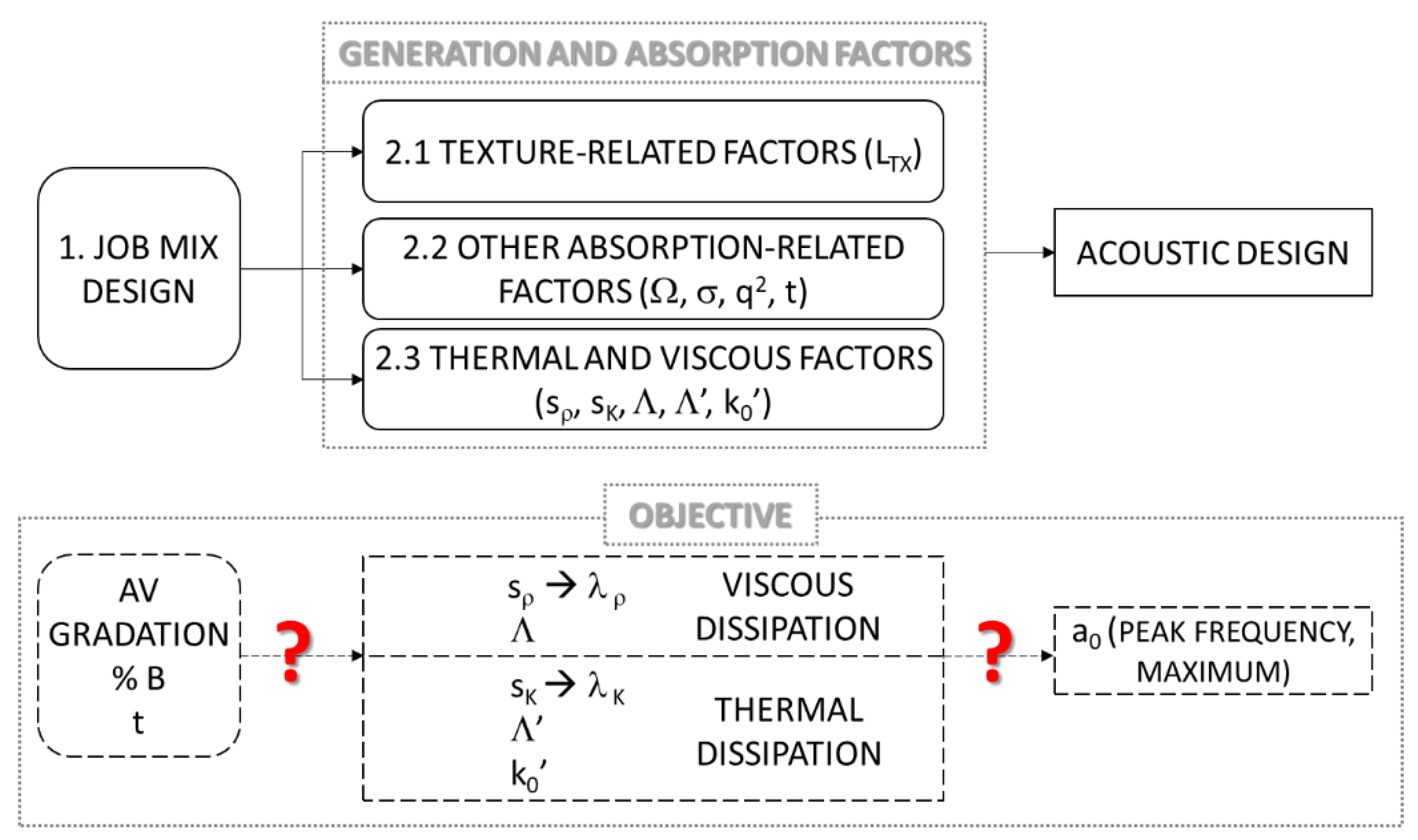
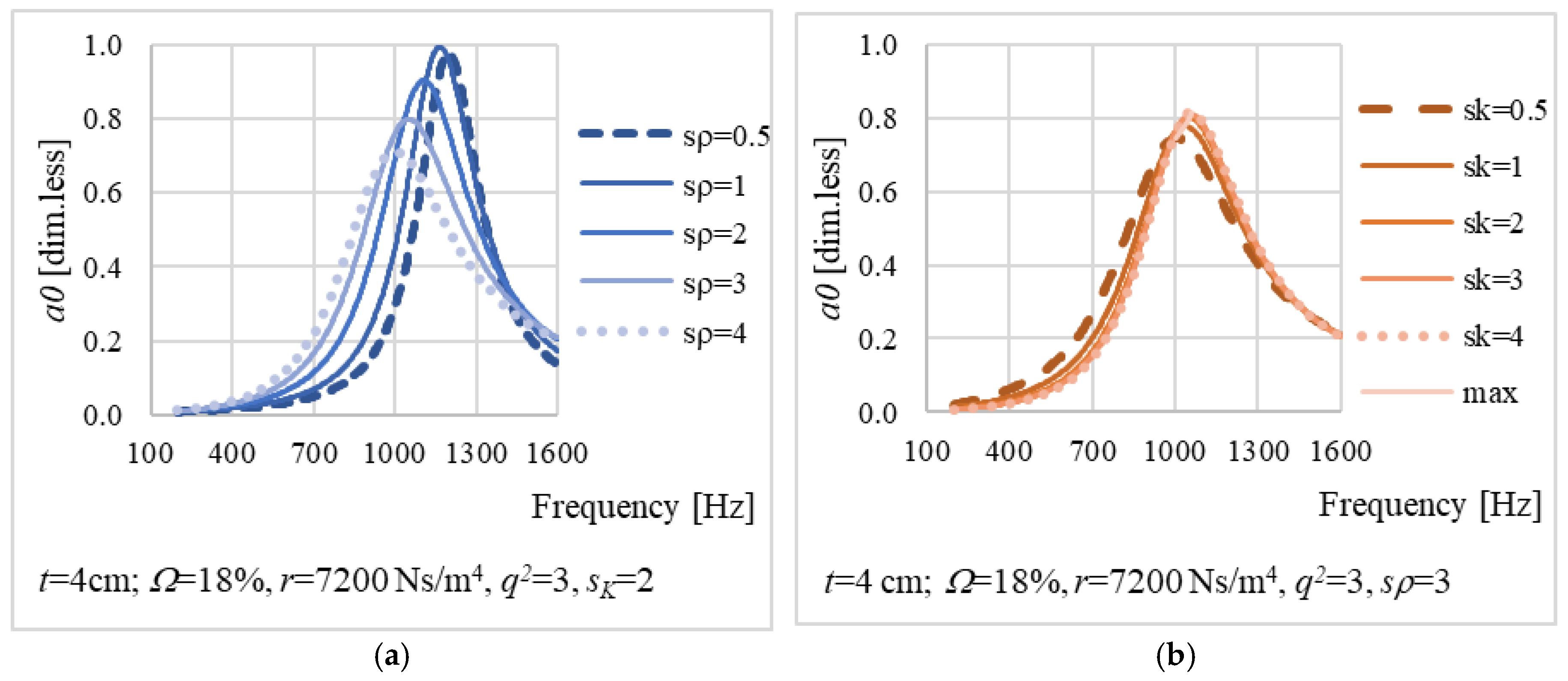
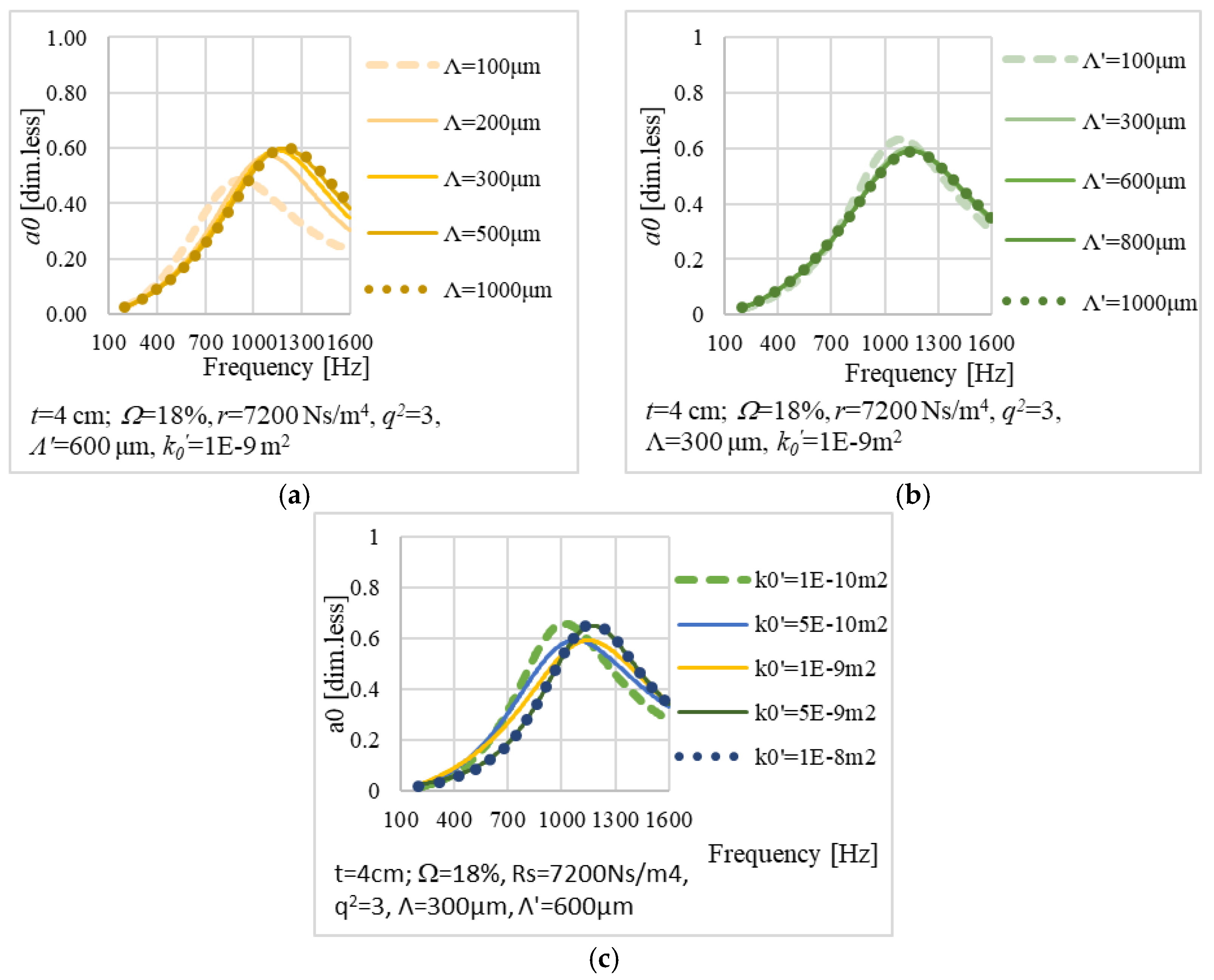
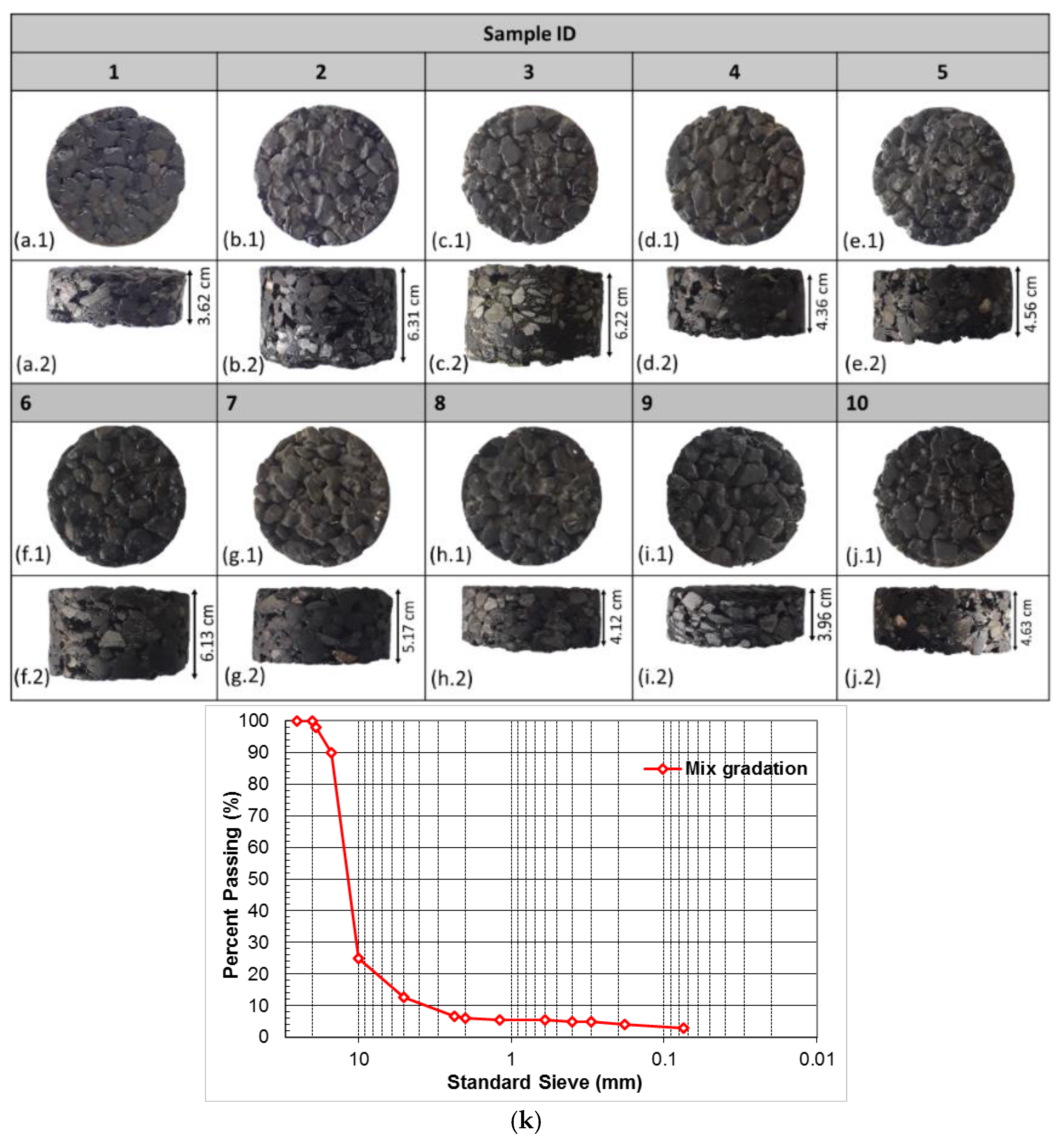
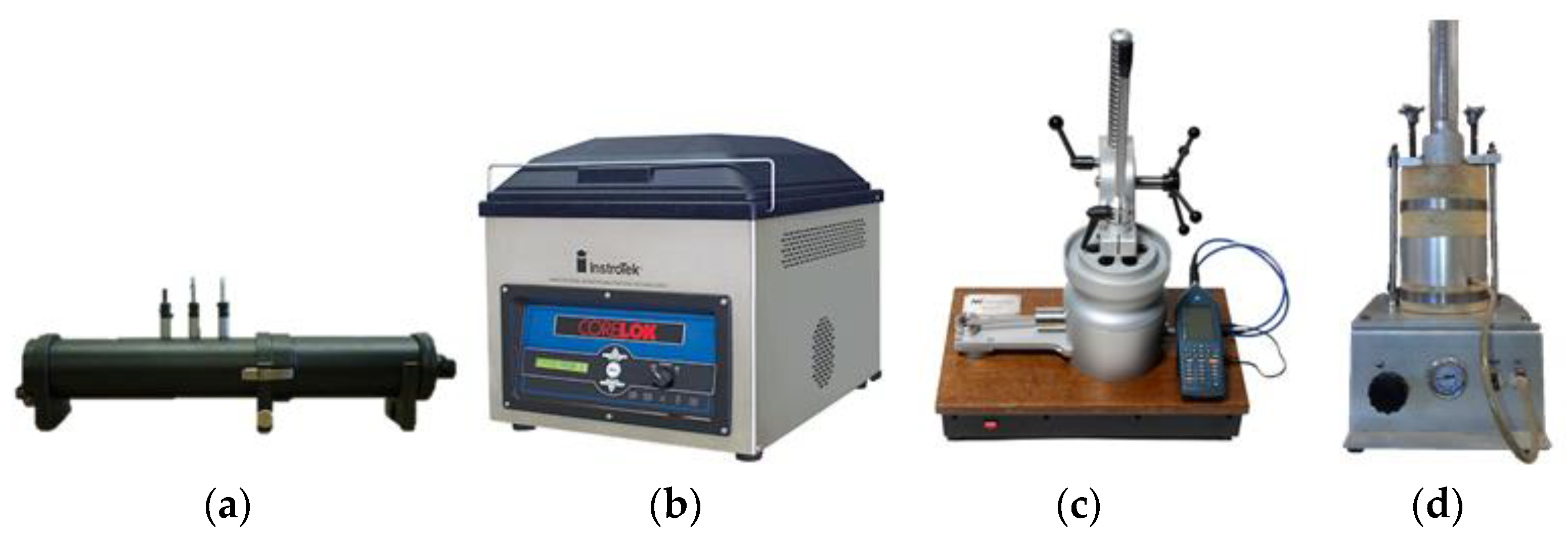
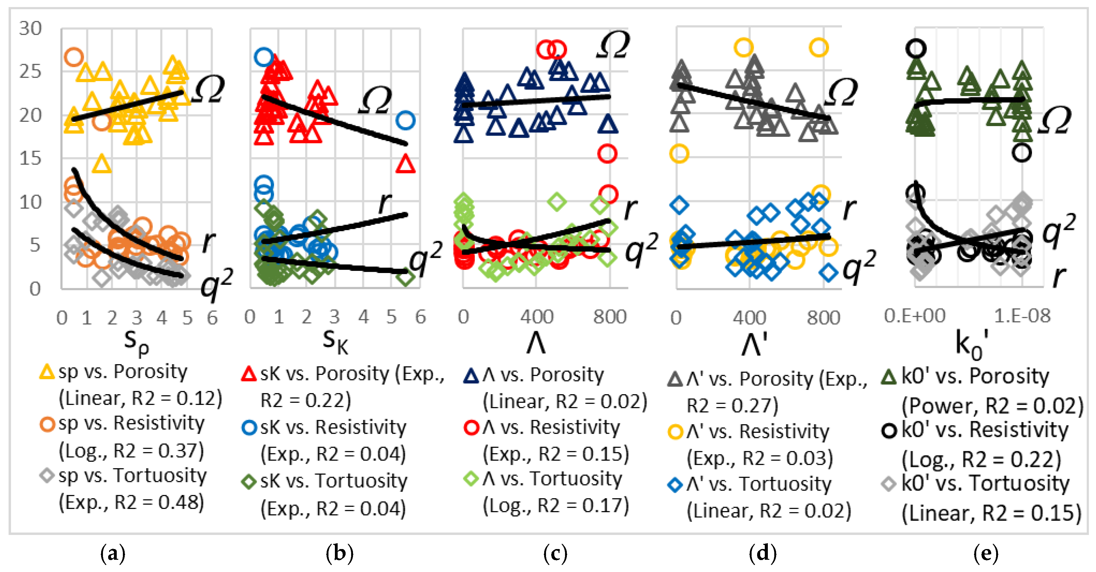
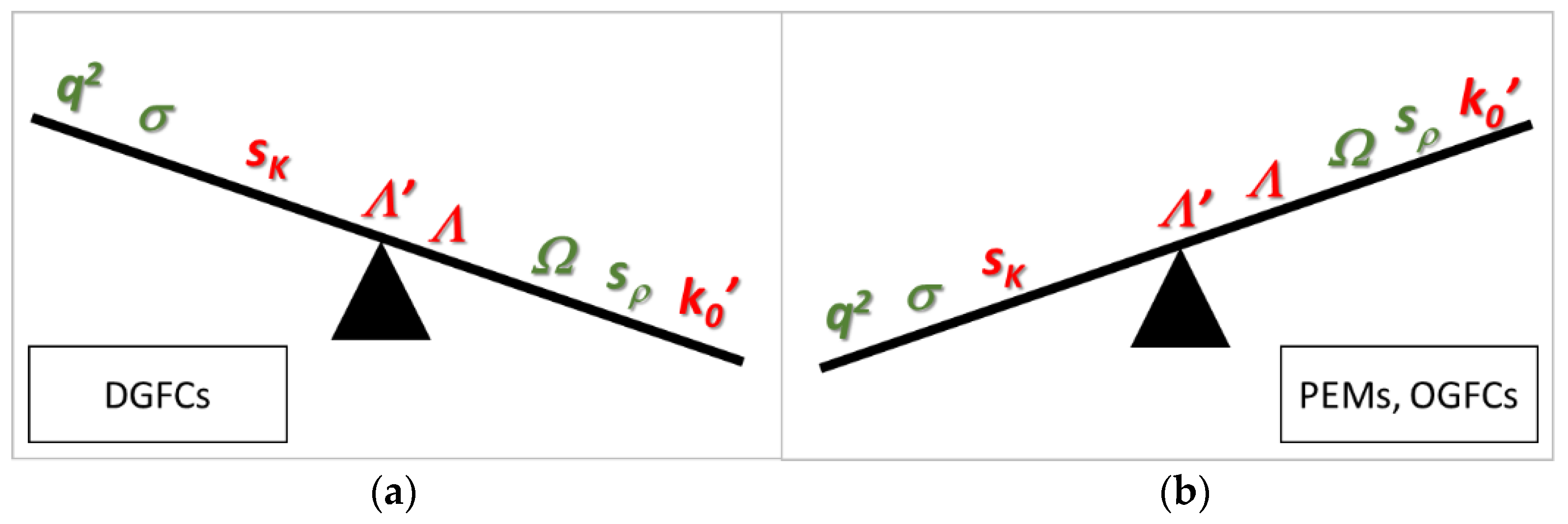
Table 1.
Values of sρ and sK of common materials.
| Ref. | Range of sρ (dim.less) | Range of sK (dim.less) | Short Notes |
|---|---|---|---|
| [52] | 1 | 1 | Porous pavement (microstructural model with core samples. d = 10 cm; t = 4 cm; r = 55,000 Ns/m4, Ω = 15%, q2 = 2.5). |
| [52] | 1.14 | 0.44 | Porous asphalt (microstructural model/Circular pores. r = 55,000 Ns/m4, Ω = 15%, q2 = 2.5). |
| [52] | 1.14 | 0.88 | Porous asphalt (microstructural model constant cross-section with a modification of the shape along the pore axis. r = 55,000 Ns/m4, Ω = 15%, q2 = 2.5). |
| [75] | 3.1 | 0.350 | Porous absorber made up of ground tire rubber (GTR), vermiculite and expanded polystyrene (EPS. r = 8865 Ns/m4, Ω = 61.7%, q2 = 2.749, D = 408.7 kg/m3, binder concentration 5%, grain size < 2.0 mm). |
| [75] | 2.590 | 0.285 | Porous absorber GTR 88% (r = 14,551 Ns/m4, Ω = 53.5%, q2 = 2.402, D = 547.6 kg/m3, binder concentration 12% grain size 1.0–3.0 mm). |
| [51] | 0.93 | 5.15 | Two-diameter model porous material (i.e., a specially fabricated sample consisting of two porous layers with two different diameters, i.e., about 1.5 mm and about 0.3 mm. r = 68.7 cgs rayls/cm, Ω = 39.2%, q2 = 4.06). |
| [76] | 1.2–1.34 | 0.83–0.9 | Loose aquarium gravel (r = 4850 ± 626 Ns/m4, Ω = 43.4% ± 0.24%, q2 = 1.37 ± 0.17, layer 1 t = 5 ± 0.2 cm and layer 2 t = 10 ± 0.2 cm). |
| [72] | 0.408–0.816 (rectangular pores) −0.548–1.095 (triangular pores) | n.a. | Two model porous materials were built. The first one containing rectangular pores (about 0.15 × 0.17 mm; Ω = 0.9, q2 = 1.44, and r = 8.71 cgs rayl/cm). The second one containing triangular pores (about 0.34 × 0.37 mm. Ω = 0.3, q2 = 1.44, and r = 14.2 cgs rayl/cm). |
Symbols. Ref. reference; sρ = viscous pore shape factor; sK = thermal pore shape factor; d = diameter; t = thickness; r = airflow resistivity; D = bulk density; Ω = porosity; q2 = tortuosity; n.a. = not available.
Table 2.
Values of Λ, Λ′, and k0′ for common materials.
| Ref. | Range of Λ (μm) | Range of Λ′ (μm) | Range of k0′ (m2) | Short Notes |
|---|---|---|---|---|
| [89] | 0.73–1.2 | 64–100 | n.a. | Composite materials made of adhesive mortar and scrap tire rubber particles (E = 281–6140 MPa; D = 0.92–1.52 g/cm3; t = 0.5–0.58 cm; Ω = 44–83%; q2 = 1.5–3.5, r = 3 × 10³–26 × 105 Ns/m4). |
| [90] | 30–182 | 60–400 | n.a. | Fibrous materials (felt, fiberglass, polyester fibers). q2 = 1–1.06. |
| [90] | 5–450 | 15–690 | n.a. | Cellular materials (cellular rubber, melamine foam, metal foam, plastic foam, poroelastic foam, polymide foam, polylactide and polyethylene glycol foam, polyurethane foam). q2 = 1.01–4.45. |
| [90] | 5.1–550 | 15.4–830 | n.a. | Granular materials (lead shot, gravel, glass breads, perlite; t = 0.01–0.9 cm; q2 = 1.1–3.84). Other q2: Open porous asphalt = 2–3.3. Asphalt = 1.8. Compacted soil = 1.4. Forest floor = 1.1. Soft soil = 1.3. Snow old crusted = 4. Snow new = 1.5–2.7. |
| [90] | 49–770 | 131–582 | n.a. | Porous aluminum, porous ceramic, snow. q2 = 1.1–3.3. |
| [91] | 104–154 7–45 55–69 38–72 | 104–292 112–368 78–142 84–392 | n.a. | Four materials are frequently used in aerospace and building applications for thermal and sound insulation. Material A (Low resistivity plastic foam. t = 5 cm; Ω = 98%; D = 9 kg/m3; r = 1 × 10⁴ Ns/m4; q2 = 1–1.07); Material B (High airflow resistivity plastic foam. t = 5 cm; Ω = 99%; D = 5 kg/m3; r = 4 × 10⁴ Ns/m4; q2 = 1–2.6); Material C (Low density fibrous materials. t = 1.8 cm; Ω = 99%; D = 5.5 kg/m3; r = 1.5 × 10⁴ Ns/m4; q2 = 1–1.05); Material D (High-density fibrous materials. t = 8 cm; Ω = 99%; D = 40 kg/m3; r = 1.3 × 10⁴ Ns/m4; q2 = 1–1.15). |
| [92] | 420 790 300 370 | 830 260 940 810 | n.a. | 3D-printed specimens. Sample 1: body centered cubic, BCC (t = 6 cm; Ω = 80%; r = 1.3 × 10³ Ns/m4; q2 = 1.52). Sample 2: BCC (t = 5 cm; Ω = 71%; r = 7 × 10³ Ns/m4; q2 = 2.55). Sample 3: face centered cubic, FCC (t = 6.5 cm; Ω = 77%; r = 4.3 × 10³ Ns/m4; q2 = 2). Sample 4: similar to Weaire–Phelan structure, A15 (t = 6.5 cm; Ω = 77%; r = 2.3 × 10³ Ns/m4; q2 = 2). |
| [93] | 245–251 | 418–430 | n.a. | Date palm fibers (t = 2–4 cm; D = 65 kg/m3; r = 0.91 × 10³–1 × 10³ Ns/m4; Ω = 93%; q2 = 2.9). |
| [94] | 120 | 500 | n.a. | Reticulated foams (q2 = 1.2; Ω = 98%; r = 4 × 10⁴ Ns/m4). |
| [84] | 180–202 132–134 249–273 | 429–610 292–370 650–750 | n.a. | Helium saturated sample measured at ultrasonic frequencies (70–600 kHz). Sample 1: t = 1 cm; Ω = 98%; q2 = 1.052. Sample 2: t = 0.9 cm; Ω = 97%; q2 = 1.042. Sample 3: t = 0.9 cm; Ω = 97%; q2 = 1.054. |
| [82] | 199 (with c = 0.56) 147 (with c = 0.94) | 291 (with c′ = 2.6) 287 (with c′ = 2.1) | n.a. | Ultrasonic measurements on air-filled porous samples. Sample 1: t = 0.2–1 cm; Ω = 98%; q2 = 1.06. Sample 2: t = 0.2–0.9 cm; Ω = 97%; q2 = 1.12. Air characteristics: D = 1.2 kg/m3; η = 1.85 × 10⁻⁵ kg/m × s; γ = 1.4; Npr = 0.71. |
| [79] | 610 (with c = 0.3) 2100 (with c = 0.03) | 1.3 × 10⁻⁸–1.7 × 10⁻⁸ | Measurements of dynamic compressibility of air-filled porous materials at audible frequencies. Foam (r = 6 × 10³ Ns/m4; Λ = 0.3 × 10⁻⁸ m2; k0′ = 1.3 × 10⁻⁸ m2). Glass wool (r = 2.3 × 10³ Ns/m4; Λ = 0.8 × 10⁻⁸ m2; k0′ = 1.7 × 10⁻⁸ m2). | |
| [95] | 226 37 | 226 121 | n.a. | Rigid open-cell porous materials (partially reticulated foams). Sample 1: Ω = 90%; q2 = 7.8; r = 25 × 103 Ns/m4. Sample 2: Ω = 99%; q2 = 1.98; r = 65 × 103 Ns/m4. |
| [83] | 197–209 19.7–20.3 7–7.2 | n.a. | n.a. | Polyurethane foam (Low r = 2.3 × 10³ Ns/m4; Ω = 96%; q2 = 1.29). Metal foam (Medium r = 50 × 103 Ns/m4; Ω = 89%; q2 = 1.27). Rock wool (High r = 150 × 103 Ns/m4; Ω = 93%; q2 = 1). Air characteristics: D = 1.15–1.19 kg/m3; η = 1.83 × 10⁻⁵–1.84 × 10⁻⁵ Ns/m2. |
| [87] | n.a. | 340–400 (with c′ = 0.98) 120–145 (with c′ = 1.34) 51–67 (with c′ = 2.84) | 11 × 10−10–206 × 10−10 | Polyurethane foam (t = 1.3 cm; r = 2.3 × 10³ Ns/m4; Ω = 96%; q2 = 1.28; D = 60 kg/m3; k0′ = 120 × 10−10–200 × 10−10 m2). Glass wool (t = 1.2 cm; r = 24.3 × 10³ Ns/m4; Ω = 98%; q2 = 1.01; D = 53 kg/m3; k0′ = 28 × 10−10–34 × 10−10 m2). Rock wool (t = 1.1 cm; r = 51.2 × 10³ Ns/m4; Ω = 97%; q2 = 1.06; D = 183 kg/m3; k0′ = 13 × 10−10–14 × 10−10 m2). |
| [96] | 76–96 190–222 54–80 | n.a. | n.a. | Industrial method (low-frequency ultrasound) to quickly measure tortuosity and viscous characteristic length. Glass beads (t = 1.3–2.15 cm; q2 = 1.37–1.4). Plastic foam (t = 1.3 cm; r = 3.6 × 10³ Ns/m4; q2 = 1.06; Ω = 99%). Felt (t = 1.8 cm; r = 26 × 103 Ns/m4; q2 = 1; Ω = 98%). |
| [97] | 1000 | 1850 | 4.8 × 10⁻⁸–9.16 × 10⁻⁸ | Open-cell aluminum foam (Ω = 92%). |
| [98] | 5–200 77–155 | 5–400 207–240 | n.a. | Industrial data related to a wide variety of porous materials (Ω = 70–99%; r = 1.5 × 10³–2 × 10⁵ Ns/m4; q2 = 1–3). Polyurethane foam (Ω = 95–97%; r = 14 × 103–17 × 103 Ns/m4; q2 = 1.6–2.3). |
| [99] | 51–240 | 51–240 | n.a. | Theoretical materials (t = 1.3–4.5 cm; Ω = 55–95%; q2 = 1–33.2; r = 12 × 103–1 × 10⁵ Ns/m4. |
| [100] | 47–69 | 159–196 | n.a. | Polyurethane foam (D = 66.22 Kg/m3; r = 24.2–57.8 Ns/m4; Ω = 95%; E = 61 kPa; q2 = 3.2–3.6). |
| [101] | 155–160 | 310–320 | 2.9 × 10⁻⁹–3.1 × 10⁻⁹ | Foam-formed cellulose materials (D = 37.3–38.18 kg/m3; Ω Ω = 98.3–98.5%; r = 5770–6200 Ns/m4; q2 = 1.007–1.009). |
Symbols. Ref. = reference; Λ = viscous characteristic length; Λ′ = thermal characteristic length; k0′ = static thermal permeability; t = thickness; r = airflow resistivity; D = bulk density; Ω = porosity; q2 = tortuosity; E = Young’s modulus; Npr = Prandtl number; η = dynamic viscosity; γ = specific heat ratio; n.a. = not available.
| Case | Parameters | If | Then | Average First Derivatives |
|---|---|---|---|---|
| 1 | t = 4 cm, Ω = 18%, r = 7200 Ns/m4, q2 = 3, sρ = 0.5–4.0, sK = 2 | sρ↑ | a0,max ↓ f (a0,max) ↓ | −0.0150 Hz−1 |
| 2 | t = 4 cm, Ω = 18%, r = 7200 Ns/m4, q2 = 3, sρ = 3, sK = 0.5–4.0 | sK↑ | a0,max ↑ f (a0,max) ↑ | 0.00130 Hz−1 |
| 3 | t = 4 cm, Ω = 18%, r = 7200 Ns/m4, q2 = 3, Λ = 100–1000 μm, Λ′ = 600 μm, k0′ = 1 × 10⁻⁹ m2 | Λ↑ | a0,max ↑ f (a0,max) ↑ | 0.00040 μmHz−1 |
| 4 | t = 4 cm, Ω = 18%, R = 7200 Ns/m4, q2 = 3, Λ = 300 μm, Λ′ = 100–1000 μm, k0′ = 1 × 10⁻⁹ m2 | Λ′↑ | a0,max ↓ f (a0,max) ↑ | −0.0007 μmHz−1 |
| 5 | t = 4 cm, Ω = 18%, r = 7200 Ns/m4, q2 = 3, Λ = 300 μm, Λ′ = 600 μm, k0′ = 1 × 10⁻¹⁰–1 × 10⁻⁸ m2 | k0′↑ | a0,max ↓↑ f (a0,max) ↑ | −0.00002 m2 Hz−1 |
Symbols. t = thickness; Ω = porosity; r = airflow resistivity; q2 = tortuosity; sρ = viscous pore shape factor; sK = thermal pore shape factor; Λ = viscous characteristic length; Λ′ = thermal characteristic length; k0′ = static thermal permeability; fmax = frequency associated with maximum of the sound absorption spectrum; a0,max = maximum of the sound absorption coefficient spectrum; ↓ = decrease; ↑ = increment; ↓↑ = constancy.
Table 4.
Main parameters of the samples derived during the in-lab measurements.
| # | t (cm) | AV (%) | Ωc (%) | a0,max (dim.less) | f (a0,max) (Hz) | rmeas_UP (Ns/m4) | rmeas_LOW (Ns/m4) | k20 (cm/s) |
|---|---|---|---|---|---|---|---|---|
| 1 | 3.62 | 22.47 | 20.88 | 0.82 | 1182 | 3911 | 3633 | 0.21 |
| 2 | 6.31 | 18.53 | 16.94 | 0.78 | 1004 | 77,983 | 5333 | 0.02 |
| 3 | 6.22 | 15.33 | 16.02 | 0.80 | 1278 | 25,837 | 4089 | 0.05 |
| 4 | 4.36 | 23.67 | 20.81 | 0.85 | 1118 | 3472 | 3798 | 0.25 |
| 5 | 4.56 | 26.47 | 24.47 | 0.87 | 986 | 1858 | 1871 | 0.44 |
| 6 | 6.13 | 24.99 | 24.67 | 0.89 | 806 | 2733 | 2242 | 0.38 |
| 7 | 5.17 | 24.52 | 22.14 | 0.76 | 862 | 1966 | 2068 | 0.34 |
| 8 | 4.12 | 23.10 | 22.13 | 0.92 | 1068 | 2416 | 2484 | 0.28 |
| 9 | 3.96 | 24.90 | 20.62 | 0.81 | 1102 | 2750 | 2832 | 0.27 |
| 10 | 4.63 | 25.65 | 23.76 | 0.84 | 1020 | 2416 | n.a. | 0.28 |
| Standards | - | [102] | [102,103] | [104] | - | [105] | [105] | [106] |
Symbols. t = thickness; AV = air void content; Ωc = porosity from corelok machine (Figure 5b); a0,max = maximum of the sound absorption spectrum measured using the Kund’t tube (Figure 5a); f(a0,max) = frequency corresponding to a0,max; rmeas_UP and rmeas_LOW = airflow resistivity measured using the instrument in Figure 5c from the upper, UP, and the lower, LOW, surface of the samples; k20 = permeability at 20 °C measured using the instrument in Figure 5d; dim.less = dimensionless.
Table 5.
Values of the main parameters and goodness of fit of the models STIN and JCAL (optimization: 600–1600 Hz).
Table 5.
Values of the main parameters and goodness of fit of the models STIN and JCAL (optimization: 600–1600 Hz).
| Case | N. of Layers | Model | |||||||
| STIN | Simulation Goodness | ||||||||
| t (cm) | Ω(%) (dim.less) | rest (kNs/m4) | q2 (dim.less) | sρ (dim.less) | sK (dim.less) | STIN | |||
| 1 | 1L | 3.62 | 17.88 | 7.22 | 2.92 | 3.23 | 2.18 | Good | |
| 2L (UP) | 1.75 | 21.76 | 6.15 | 1.52 | 4.26 | 1.03 | Good | ||
| 2L (LOW) | 1.87 | 20.00 | 5.75 | 7.87 | 2.25 | 0.87 | |||
| 2 | 1L | 6.31 | 14.45 | 19.31 | 1.24 | 1.62 | 5.49 | Good | |
| 2L (UP) | 3.26 | 19.94 | 26.69 | 5.07 | 0.50 | 0.50 | Bad | ||
| 2L (LOW) | 3.05 | 13.94 | 35.84 | 10.00 | 5.50 | 0.50 | |||
| 3 | 1L | 6.22 | 19.02 | 11.92 | 9.23 | 0.50 | 0.50 | Bad | |
| 2L (UP) | 3.02 | 19.02 | 10.84 | 4.03 | 0.50 | 0.50 | Bad | ||
| 2L (LOW) | 3.20 | 13.02 | 20.12 | 10.00 | 5.50 | 0.50 | |||
| 4 | 1L | 4.36 | 17.81 | 6.20 | 2.21 | 2.95 | 1.75 | Good | |
| 2L (UP) | 2.43 | 21.26 | 5.08 | 1.51 | 3.77 | 2.18 | Good | ||
| 2L (LOW) | 1.93 | 20.03 | 4.91 | 6.31 | 2.98 | 2.53 | |||
| 5 | 1L | 4.56 | 21.47 | 4.27 | 2.57 | 2.90 | 0.52 | Good | |
| 2L (UP) | 2.67 | 25.22 | 3.72 | 1.79 | 4.68 | 1.15 | Good | ||
| 2L (LOW) | 1.89 | 25.15 | 3.31 | 7.65 | 1.65 | 0.86 | |||
| 6 | 1L | 6.13 | 21.67 | 4.73 | 2.21 | 2.30 | 0.72 | Good | |
| 2L (UP) | 3.07 | 25.88 | 4.08 | 1.26 | 4.43 | 0.88 | Good | ||
| 2L (LOW) | 3.06 | 25.03 | 3.60 | 5.64 | 0.94 | 1.04 | |||
| 7 | 1L | 5.17 | 20.39 | 4.40 | 2.13 | 4.25 | 0.60 | Good | |
| 2L (UP) | 2.06 | 22.23 | 4.16 | 2.69 | 4.20 | 2.76 | Good | ||
| 2L (LOW) | 3.11 | 21.33 | 4.03 | 2.24 | 2.92 | 2.43 | |||
| 8 | 1L | 4.12 | 19.13 | 5.88 | 3.04 | 2.24 | 1.68 | Good | |
| 2L (UP) | 1.91 | 23.51 | 4.98 | 1.45 | 3.52 | 0.71 | Good | ||
| 2L (LOW) | 2.21 | 21.69 | 4.57 | 7.81 | 1.22 | 0.81 | |||
| 9 | 1L | 3.96 | 17.63 | 6.08 | 2.75 | 2.85 | 0.50 | Good | |
| 2L (UP) | 2.12 | 22.24 | 5.46 | 1.54 | 4.77 | 0.60 | Good | ||
| 2L (LOW) | 1.84 | 20.87 | 4.88 | 8.50 | 2.24 | 0.82 | |||
| 10 | 1L | 4.63 | 20.76 | 5.75 | 2.27 | 3.04 | 0.99 | Good | |
| 2L (UP) | 2.70 | 24.67 | 5.08 | 1.39 | 4.57 | 0.71 | Good | ||
| 2L (LOW) | 1.93 | 22.94 | 4.47 | 7.96 | 2.33 | 2.40 | |||
| Standard dev. | |||||||||
| 1L | 1.0 | 2.2 | 4.7 | 2.2 | 1.0 | 1.5 | |||
| 2L (UP) | 0.5 | 2.2 | 7.0 | 1.3 | 1.6 | 0.8 | |||
| 2L (LOW) | 0.6 | 4.1 | 10.6 | 2.3 | 1.6 | 0.8 | |||
| Case | N. of Layers | JCAL | Simulation Goodness | ||||||
| t (cm) | Ω(%) (dim.less) | rest (kNs/m4) | q2 (dim.less) | Λ (μm) | Λ′ (μm) | k0′ (m2) | JCAL | ||
| 1 | 1L | 3.62 | 18.53 | 5.59 | 3.04 | 301.7 | 564.0 | 9 × 10⁻¹⁰ | Good |
| 2L (UP) | 1.87 | 23.88 | 5.59 | 9.63 | 746.1 | 15.0 | 1 × 10⁻⁸ | Good | |
| 2L (LOW) | 1.75 | 17.88 | 5.59 | 10.00 | 5.0 | 718.7 | 1 × 10⁻⁸ | ||
| 2 | 1L | 6.31 | 19.94 | 27.57 | 10.00 | 510.3 | 776.2 | 1 × 10⁻¹⁰ | Bad |
| 2L (UP) | 3.46 | 19.35 | 27.57 | 3.64 | 451.9 | 366.1 | 1 × 10⁻¹⁰ | Good | |
| 2L (LOW) | 2.85 | 14.97 | 27.57 | 9.87 | 24.5 | 451.3 | 1 × 10⁻⁸ | ||
| 3 | 1L | 6.22 | 19.02 | 10.84 | 7.03 | 789.6 | 787.0 | 1 × 10⁻¹⁰ | Bad |
| 2L (UP) | 2.79 | 19.00 | 15.48 | 3.50 | 787.9 | 15.1 | 1 × 10⁻⁸ | Bad | |
| 2L (LOW) | 3.43 | 13.03 | 15.48 | 7.63 | 86.8 | 816.5 | 1 × 10⁻¹⁰ | ||
| 4 | 1L | 4.36 | 18.71 | 4.86 | 1.82 | 176.4 | 827.9 | 4 × 10⁻¹⁰ | Good |
| 2L (UP) | 2.76 | 21.13 | 4.86 | 4.82 | 624.0 | 22.2 | 1 × 10⁻⁸ | Good | |
| 2L (LOW) | 1.60 | 20.47 | 4.86 | 7.33 | 6.2 | 677.5 | 1 × 10⁻⁸ | ||
| 5 | 1L | 4.56 | 22.43 | 3.30 | 2.52 | 242.8 | 402.2 | 1 × 10⁻⁹ | Good |
| 2L (UP) | 3.25 | 25.07 | 3.30 | 4.72 | 522.5 | 25.4 | 1 × 10⁻⁸ | Good | |
| 2L (LOW) | 1.31 | 22.45 | 3.30 | 9.27 | 7.7 | 645.7 | 1 × 10⁻⁸ | ||
| 6 | 1L | 6.13 | 24.05 | 3.65 | 2.46 | 388.6 | 318.9 | 8 × 10⁻⁹ | Bad |
| 2L (UP) | 4.26 | 25.75 | 3.65 | 4.04 | 515.1 | 425.7 | 1 × 10⁻¹⁰ | Good | |
| 2L (LOW) | 1.87 | 23.86 | 3.65 | 5.20 | 6.6 | 409.2 | 2 × 10⁻⁹ | ||
| 7 | 1L | 5.17 | 21.65 | 3.98 | 2.27 | 140.7 | 435.9 | 1 × 10⁻⁸ | Good |
| 2L (UP) | 3.21 | 24.43 | 3.98 | 5.39 | 349.3 | 32.8 | 5 × 10⁻⁹ | Good | |
| 2L (LOW) | 1.96 | 21.57 | 3.98 | 5.65 | 5.9 | 321.1 | 7 × 10⁻⁹ | ||
| 8 | 1L | 4.12 | 19.14 | 4.54 | 2.99 | 412.3 | 487.3 | 1 × 10⁻⁹ | Good |
| 2L (UP) | 2.76 | 23.65 | 4.54 | 5.67 | 695.4 | 27.4 | 5 × 10⁻⁹ | Good | |
| 2L (LOW) | 1.36 | 20.55 | 4.54 | 8.73 | 6.1 | 510.1 | 9 × 10⁻⁹ | ||
| 9 | 1L | 3.96 | 18.53 | 4.69 | 2.92 | 309.5 | 486.5 | 9 × 10⁻¹⁰ | Good |
| 2L (UP) | 2.55 | 22.31 | 4.69 | 6.32 | 592.0 | 51.4 | 7 × 10⁻⁹ | Good | |
| 2L (LOW) | 1.41 | 19.81 | 4.69 | 8.35 | 6.8 | 436.7 | 8 × 10⁻⁹ | ||
| 10 | 1L | 4.63 | 20.76 | 4.48 | 2.06 | 185.5 | 518.6 | 7 × 10⁻¹⁰ | Good |
| 2L (UP) | 2.85 | 25.07 | 4.48 | 5.39 | 578.6 | 423.5 | 1 × 10⁻¹⁰ | Good | |
| 2L (LOW) | 1.78 | 23.18 | 4.48 | 5.59 | 6.92 | 414.5 | 5 × 10⁻⁹ | ||
| Standard dev. | |||||||||
| 1L | 1.0 | 1.9 | 7.4 | 2.7 | 194.5 | 176.6 | 4 × 10⁻⁹ | ||
| 2L (UP) | 0.6 | 2.4 | 7.8 | 1.8 | 134.6 | 183.6 | 4 × 10⁻⁹ | ||
| 2L (LOW) | 0.7 | 3.5 | 7.8 | 1.8 | 25.5 | 162.9 | 4 × 10⁻⁹ | ||
Symbols. Case 1 to Case 10: ten samples under test; T = thickness of the samples; Ω = porosity; rest = airflow resistivity estimated using the Equation (17); q2: tortuosity; sρ = viscous pore shape factor (STIN model); sK = thermal pore shape factor (STIN model); Λ = viscous characteristic length (JCAL model); Λ′ = thermal characteristic length (JCAL model); k0′ = static thermal permeability (JCAL model).
Table 6.
Pearson coefficients (all cases).
| Models | STIN | JCAL | ||||||||||||
|---|---|---|---|---|---|---|---|---|---|---|---|---|---|---|
| Parameters | t | Ω | rest | q2 | sρ | sK | t | Ω | rest | q2 | Λ | Λ′ | k0′ | |
| STIN | t | 1.00 | −0.39 | 0.19 | −0.20 | −0.24 | 0.14 | 0.93 | −0.17 | 0.25 | −0.40 | 0.18 | 0.40 | −0.47 |
| Ω | −0.39 | 1.00 | −0.69 | −0.31 | −0.04 | −0.21 | −0.33 | 0.89 | −0.65 | −0.15 | 0.11 | −0.47 | 0.20 | |
| rest | 0.19 | −0.69 | 1.00 | 0.40 | 0.05 | −0.01 | 0.19 | −0.64 | 0.94 | 0.29 | 0.01 | 0.22 | −0.15 | |
| q2 | −0.20 | −0.31 | 0.40 | 1.00 | −0.24 | −0.25 | −0.34 | −0.57 | 0.28 | 0.54 | −0.52 | 0.48 | 0.15 | |
| sρ | −0.24 | −0.04 | 0.05 | −0.24 | 1.00 | −0.08 | −0.04 | 0.05 | −0.14 | 0.03 | 0.02 | −0.24 | 0.11 | |
| sK | 0.14 | −0.21 | −0.01 | −0.25 | −0.08 | 1.00 | 0.13 | 0.07 | 0.18 | 0.18 | −0.05 | 0.15 | −0.10 | |
| JCAL | t | 1.00 | −0.06 | 0.24 | −0.45 | 0.38 | 0.25 | −0.51 | ||||||
| Ω | −0.06 | 1.00 | −0.55 | −0.20 | 0.28 | −0.54 | 0.11 | |||||||
| rest | 0.24 | −0.55 | 1.00 | 0.31 | 0.12 | 0.20 | −0.16 | |||||||
| q2 | −0.45 | −0.20 | 0.31 | 1.00 | −0.17 | 0.17 | 0.38 | |||||||
| Λ | 0.38 | 0.28 | 0.12 | −0.17 | 1.00 | −0.49 | −0.13 | |||||||
| Λ′ | 0.25 | −0.54 | 0.20 | 0.17 | −0.49 | 1.00 | −0.42 | |||||||
| k0′ | −0.51 | 0.11 | −0.16 | 0.38 | −0.13 | −0.42 | 1.00 | |||||||
Table 7.
Pearson coefficients (without outliers).
| Models | STIN | JCAL | ||||||||||||
|---|---|---|---|---|---|---|---|---|---|---|---|---|---|---|
| Parameters | t | Ω | rest | q2 | sρ | sK | t | Ω | rest | q2 | Λ | Λ′ | k0′ | |
| STIN | t | 1.00 | −0.52 | 0.34 | −0.22 | −0.25 | 0.14 | 0.93 | −0.24 | 0.32 | −0.41 | 0.18 | 0.42 | −0.49 |
| Ω | −0.52 | 1.00 | −0.52 | 0.01 | 0.35 | −0.42 | −0.44 | 0.82 | −0.53 | 0.05 | −0.06 | −0.43 | 0.24 | |
| rest | 0.34 | −0.52 | 1.00 | 0.05 | −0.51 | 0.21 | 0.34 | −0.41 | 0.97 | 0.06 | 0.33 | 0.18 | −0.36 | |
| q2 | −0.22 | 0.01 | 0.05 | 1.00 | −0.65 | −0.17 | −0.38 | −0.36 | 0.02 | 0.46 | −0.47 | 0.44 | 0.18 | |
| sρ | −0.25 | 0.35 | −0.51 | −0.65 | 1.00 | 0.02 | −0.03 | 0.54 | −0.52 | −0.16 | 0.17 | −0.42 | 0.14 | |
| sK | 0.14 | −0.42 | 0.21 | −0.17 | 0.02 | 1.00 | 0.13 | −0.08 | 0.34 | 0.26 | −0.10 | 0.21 | −0.11 | |
| JCAL | t | 1.00 | −0.10 | 0.31 | −0.47 | 0.39 | 0.26 | −0.52 | ||||||
| Ω | −0.10 | 1.00 | −0.37 | 0.00 | 0.16 | −0.51 | 0.11 | |||||||
| rest | 0.31 | −0.37 | 1.00 | 0.15 | 0.32 | 0.15 | −0.28 | |||||||
| q2 | −0.47 | 0.00 | 0.15 | 1.00 | −0.10 | 0.13 | 0.39 | |||||||
| Λ | 0.39 | 0.16 | 0.32 | −0.10 | 1.00 | −0.48 | −0.14 | |||||||
| Λ′ | 0.26 | −0.51 | 0.15 | 0.13 | −0.48 | 1.00 | −0.40 | |||||||
| k0′ | −0.52 | 0.11 | −0.28 | 0.39 | −0.14 | −0.40 | 1.00 | |||||||
Table 8.
Summary.
| Material Science | Acoustic Inputs | sρ Viscous Effects (Narrow Sections of the Pores) | sK Thermal Effects (Wider Sections of the Pores) | Λ Viscous Effects | Λ′ Thermal Effects | k0′ Thermal Effects | |||
|---|---|---|---|---|---|---|---|---|---|
| AV, neff | Ω ↑ | ↑ | ↓ | ↑ | ↓ | ↑ | |||
| K20, rest | rest ↑ | ↓ | ↑ | ↑ | ↑ | ↓ | |||
| q2 ↑ | ↓ | ↓ | ↓ | ↑ | ↑ | ||||
| Partial Equations (Two-layer Approach) | Partial Equations (Two-layer Approach) | ||||||||
| sρ (Ω) | 1L | sρ = 2.5303 ln (Ω) − 4.8488 | R2 = 0.0929 | Λ (q2) | 1L | Λ = 293.19 ln (q2) +8.6725 | R2 = 0.6781 | ||
| 2L | sρ = 1 × 10⁻⁴ Ω3.2527 | R2 = 0.1730 | 2L | Λ = 83,125 q2 − 3.902 | R2 = 0.3060 | ||||
| sK (Ω) | 1L | sK = −10.54 ln (Ω) + 32.464 | R2 = 0.7023 | Λ′ (q2) | 1L | Λ′ = 38.608 q2 + 417.18 | R2 = 0.3372 | ||
| 2L | sK = −0.0461 Ω + 2.2976 | R2 = 0.0153 | 2L | Λ′ = 55.326 q2 − 40.416 | R2 = 0.2080 | ||||
| Λ (Ω) | 1L | Λ = −464.2 ln (Ω) + 1741 | R2 = 0.0470 | k0′ (q2) | 1L | k0′ = 4 × 10⁻⁹ exp − (0.403 q2) | R2 = 0.4988 | ||
| 2L | Λ = 0.0194 exp (0.3737 Ω) | R2 = 0.1431 | 2L | k0′ = 1 × 10⁻⁹ q2 + 4 × 10⁻¹⁰ | R2 = 0.2865 | ||||
| Λ′ (Ω) | 1L | Λ′ = 6394.2 exp − (0.122 Ω) | R2 = 0.5456 | Global Equations (single-layer approach) | |||||
| 2L | Λ′ = −776.1 ln (Ω) + 2709.1 | R2 = 0.1088 | |||||||
| k0′ (Ω) | 1L | k0′ = 1 × 10⁻⁹ Ω − 2 × 10⁻⁸ | R2 = 0.4593 | ||||||
| 2L | k0′ = −7 × 10⁻¹⁰ Ω + 2 × 10⁻⁸ | R2 = 0.1807 | sρ (Ω) | sρ = 0.173 Ω−0.8927 | R2 = 0.1220 | ||||
| sρ (rest) | 1L | sρ = −1.49 ln (rest) + 5.4277 | R2 = 0.4864 | sρ (rest) | sρ = 4.0314 exp − (0.081rest) | R2 = 0.3713 | |||
| 2L | sρ = 4.0057 exp − (0.085rest) | R2 = 0.3864 | sρ (q2) | sρ = −1.362 ln (q2) + 4.2939 | R2 = 0.4784 | ||||
| sK (rest) | 1L | sK = 0.2666 rest−0.5288 | R2 = 0.6614 | sK (Ω) | sK = −3.89 ln (Ω) + 13.192 | R2 = 0.2169 | |||
| 2L | sK = 2.6293 rest−0.535 | R2 = 0.2005 | sK (rest) | sK = 0.4716 ln (rest) + 0.52 | R2 = 0.0439 | ||||
| Λ (rest) | 1L | Λ = 193.03 ln (rest) + 9.3394 | R2 = 0.4045 | sK (q2) | sK = −0.316 ln (q2) + 1.6993 | R2 = 0.0379 | |||
| 2L | Λ = 186.15 ln (rest) + 23.343 | R2 = 0.1024 | Λ (Ω) | Λ = 18.289 Ω−58.628 | R2 = 0.0249 | ||||
| Λ′ (rest) | 1L | Λ′ = 195.51 ln (rest) + 219.7 | R2 = 0.5033 | Λ (rest) | Λ = 188.93 ln (rest) + 17.961 | R2 = 0.1547 | |||
| 2L | Λ′ = 261.7 rest−0.339 | R2 = 0.0145 | Λ (q2) | Λ = 687.36 exp − (0.316 q2) | R2 = 0.1706 | ||||
| k0′ (rest) | 1L | k0′ = 2 × 10⁻⁸ rest−1.779 | R2 = 0.5654 | Λ′ (Ω) | Λ′ = −1221 ln (Ω) + 4136.4 | R2 = 0.2690 | |||
| 2L | k0′ = 7 × 10⁻⁹ exp − (0.101rest) | R2 = 0.1404 | Λ′ (rest) | Λ′ = 72.572 ln (rest) + 276.29 | R2 = 0.0257 | ||||
| sρ (q2) | 1L | sρ = 4.5752 × 10−0.224 q2 | R2 = 0.7036 | Λ′ (q2) | Λ′ = 12.945 q2 + 328.44 | R2 = 0.0170 | |||
| 2L | sρ = −1.538 ln (q2) + 4.714 | R2 = 0.6025 | k0′ (Ω) | k0′ = 3 × 10⁻¹² Ω2.1138 | R2 = 0.0183 | ||||
| sK (q2) | 1L | sK = −1.659 ln (q2) + 3.1085 | R2 = 0.3002 | k0′ (rest) | k0′ = 5 × 10⁻⁹ exp − (0.124rest) | R2 = 0.2168 | |||
| 2L | sK = 0.0322 ln (q2) + 1.2268 | R2 = 0.0009 | k0′ (q2) | k0′ = 6 × 10⁻¹⁰ q2 + 2 × 10⁻⁹ | R2 = 0.1538 | ||||
Publisher’s Note: MDPI stays neutral with regard to jurisdictional claims in published maps and institutional affiliations. |
© 2021 by the authors. Licensee MDPI, Basel, Switzerland. This article is an open access article distributed under the terms and conditions of the Creative Commons Attribution (CC BY) license (https://creativecommons.org/licenses/by/4.0/).
Share and Cite
MDPI and ACS Style
Praticò, F.G.; Fedele, R.; Briante, P.G. On the Dependence of Acoustic Pore Shape Factors on Porous Asphalt Volumetrics. Sustainability 2021, 13, 11541. https://0-doi-org.brum.beds.ac.uk/10.3390/su132011541
AMA Style
Praticò FG, Fedele R, Briante PG. On the Dependence of Acoustic Pore Shape Factors on Porous Asphalt Volumetrics. Sustainability. 2021; 13(20):11541. https://0-doi-org.brum.beds.ac.uk/10.3390/su132011541
Chicago/Turabian StylePraticò, Filippo Giammaria, Rosario Fedele, and Paolo Giovanni Briante. 2021. "On the Dependence of Acoustic Pore Shape Factors on Porous Asphalt Volumetrics" Sustainability 13, no. 20: 11541. https://0-doi-org.brum.beds.ac.uk/10.3390/su132011541
Note that from the first issue of 2016, this journal uses article numbers instead of page numbers. See further details here.