Solving Traveling Salesman Problem with Time Windows Using Hybrid Pointer Networks with Time Features

Abstract

This paper introduces a time efficient deep learning-based solution to the traveling salesman problem with time window (TSPTW). Our goal is to reduce the total tour length traveled by -*the agent without violating any time limitations. This will aid in decreasing the time required to supply any type of service, as well as lowering the emissions produced by automobiles, allowing our planet to recover from air pollution emissions. The proposed model is a variation of the pointer networks that has a better ability to encode the TSPTW problems. The model proposed in this paper is inspired from our previous work that introduces a hybrid context encoder and a multi attention decoder. The hybrid encoder primarily comprises the transformer encoder and the graph encoder; these encoders encode the feature vector before passing it to the attention decoder layer. The decoder consists of transformer context and graph context as well. The output attentions from the two decoders are aggregated and used to select the following step in the trip. To the best of our knowledge, our network is the first neural model that will be able to solve medium-size TSPTW problems. Moreover, we conducted sensitivity analysis to explore how the model performance changes as the time window width in the training and testing data changes. The experimental work shows that our proposed model outperforms the state-of-the-art model for TSPTW of sizes 20, 50 and 100 nodes/cities. We expect that our model will become state-of-the-art methodology for solving the TSPTW problems.

1. Introduction

Greenhouse gases have maintained Earth’s temperature as livable for humans and millions of other species by trapping heat from the sun. However, those gases have become out of balance, threatening the existence and survival of living beings on our planet. The level of carbon dioxide- the most hazardous and ubiquitous greenhouse gas is at a record high in the atmosphere. Burning of fossil fuels is mainly responsible for the high amounts of greenhouse gases in the atmosphere. Rather than allowing heat to escape into space, the gases absorb solar energy and hold it near to the Earth’s surface. The greenhouse effect—the result of this heat trapping, was first proposed in the 19th century by French mathematician Joseph Fourier, who estimated in 1824 that the Earth would be significantly colder if it didn’t have an atmosphere. Svante Arrhenius- a Swedish physicist, was the first to correlate an increase in carbon dioxide gas from burning fossil fuels with a warming impact in 1896. “The greenhouse effect has been recognized and is influencing our climate now”, American climate scientist James E. Hansen testified to Congress almost a century later.

Climate change is the phrase that scientists use today to describe the complex adjustments impacting our planet’s weather and climate systems as a result of rising greenhouse gas concentrations. It includes not just rising of average temperatures, which we refer to as global warming, but also extreme weather events, shifting species populations and habitats, rising sea levels, and a variety of other consequences. Governments and other organizations throughout the globe are monitoring greenhouse gases, documenting their affects, and adopting remedies, such as the Intergovernmental Panel on Climate Change (IPCC), a United Nations group that studies the latest climate change science.

Carbon dioxide is the most common greenhouse gas, accounting for around three-quarters of all emissions. It lasts for thousands of years in the atmosphere. Carbon dioxide levels at Hawaii’s Mauna Loa Atmospheric Baseline Observatory hit 411 parts per million in 2018, the highest monthly average ever measured. Burning of organic resources such as coal, oil, gas, wood, and solid waste produces most of carbon dioxide emissions.

Transport is Europe’s biggest source of CO₂, responsible for the emission of over a quarter of all greenhouse gases. Transport emissions have increased by a quarter since 1990 and are continuing to rise with 2017 oil consumption in the EU increasing at its fastest pace since 2001 [1]. Unless transport emissions are brought under control,’ National Climate Goals 2030 will not be realized. To meet the 2050 Paris climate commitments, cars and vans must be entirely decarbonized. This requires ending sales of cars with an internal combustion engine by 2035. Such a transformation requires wholesale changes, not only to vehicles but also how they are owned, taxed and driven.

Nearly half of the people in the United States—an estimated 150 million—live in locations where federal air quality requirements are not met. Passenger cars and vans (‘light commercial vehicles’) are responsible for around 12% and 2.5%, respectively, of total EU emissions of carbon dioxide (CO₂), which is the main greenhouse gas. Comprising of ozone, particulate matter, and other smog-forming pollutants. The dangers of air pollution on one’s health are enormous. Poor air quality aggravates respiratory disorders such as asthma and bronchitis, raises the risk of life-threatening diseases such as cancer, and places significant financial strain on our health-care system. It is responsible for up to 30,000 premature deaths each year.

Passenger cars are a major source of pollution, emitting large volumes of nitrogen oxides, carbon monoxide, and other pollutants. In 2013, transportation accounted for more than half of the carbon monoxide and nitrogen oxide emissions, as well as about a quarter of the hydrocarbons released into the atmosphere. We are attempting to solve this issue by reducing automotive emissions using machine learning approaches.

Machine learning is concerned with completing a task given to a set of typically limited and noisy data. It is ideally suited for natural signals when no obvious mathematical formulation arises since the real data distribution is unknown analytically, such as when processing pictures, text, speech, or molecules, or when working with recommender systems, social networks, or financial forecasts. Nowadays, one of the most exciting fields of study is solving combinatorial optimization problems using machine learning.

Combinatorial optimization is a topic at the intersection of combinatorics and theoretical computer science that seeks to tackle discrete optimization problems using combinatorial approaches. A discrete optimization problem tries to find the optimal solution from an unlimited number of solutions. It is widely utilized in industries such as transportation, supply chain, energy, banking, and scheduling, to name a few.

One of the combinatorial optimization problems is the traveling salesman problem (TSP) with time windows (TSPTW). It involves deciding the shortest path for a vehicle visiting a set of nodes/cities. Each node is visited only once, and the service at that node must begin within the time frame given by the earliest and latest times when service can begin at that node. A vehicle will wait if it arrives at a node too early. Furthermore, due dates must be observed too. The TSPTW has many real-world applications, including banking, postal delivery, and school bus routing and material-handling systems with autonomous guides.

There is a need for effective heuristics due to the problem’s complexity NP-Hard because it contains the Traveling Salesman Problem as a particular case and the limits of exact techniques to discover optimum solutions in a reasonable period when considering practical examples. Carlton and Barnes [2] investigate infeasible solutions using a tabu-search heuristic with a static penalty function. In a post-optimization phase, Gendreau et al. [3] propose an insertion heuristic based on GENIUS [4] that gradually develops and improves the route by successively removing and reintroducing nodes. Calvo [5] uses an ad hoc objective function to solve an assignment problem, then creates a viable tour by combining all identified sub-tours into a major tour, followed by a 3-opt local search method to enhance the initial feasible solution. Ohlmann and Thomas [6] recently produced the best-known results for a number of cases using compressed annealing, a variation of simulated annealing [7] that relaxes the time windows restrictions by including a variable penalty approach within a stochastic search strategy.

While research on the traveling salesman problem (TSP) has expanded fast, research on the TSPTW has remained limited. Savelsbergh [8] has shown that even finding a viable solution to the TSPTW is an NP-complete issue and has introduced inter-change heuristics as a result.

The TSPTW has a variety of solvers, ranging from exact mathematical programming techniques for small size problems to heuristic approaches. Integer and dynamic-programming techniques have been employed in exact approaches to solve the TSPTW. Christofides et al. and Baker [9,10] developed branch-and-bound algorithms for problems with up to 50 nodes that need moderately tight time windows. Dumas, Y., et al. [11] use state space-reduction techniques to expand prior dynamic-programming approaches, allowing them to solve problems with up to 200 clients. In an alternate approach, Pesant et al. use constraint programming to develop an exact method [12] and a heuristic [13] for the TSPTW.

Constraint-based combinatorial optimization problems, such as TSP with time window, have not been thoroughly investigated in the literature of reinforcement learning (RL). Qiang Ma et al. [14] used RL to train a pointer network with input graph layer [15] to tackle this problem. However, their approach is still incapable of determining the optimum policy across a wide range of problem sizes, as their study only addresses up to 20 points.

In this paper, we developed a deep learning model that was trained using RL to solve TWTSP. We have re-defined the system state, rewarding schemes, and masking policy for TWTSP based on the architecture described in [1].We will follow the same approach as in [14], however the issue occurs when we need to simulate the data for training. Since we are dealing with a constrained problem, we have no guarantee that the generated data has a feasible solution. Qiang Ma [14] tackled this issue by first finding a good unconstrained TSP tour using the generated and the 2-opt local search and then generating the time window for the solved data, but there are two issues here:

• 2-opt isn’t an exact algorithm so the generated data won’t be solved optimally.
• This method does not take advantage of GPU parallelization, therefore model training will be excruciatingly slow.

We addressed these issues by changing the way we generate the data; instead of using a 2-opt model to solve the unconstrained TSP, we utilized Hybrid pointer network HPN [1] since it gives a closer to optimum solution for data ranging from 20 to 100 points. Using an HPN that is pretrained to solve unconstrained TSP will allow us to take advantage of GPU, therefor the training is not slow. By filling these gaps and modifying HPN to be able to encode time features, we will solve up to 100 points in TWTSP, whereas the previous work [14] only solves 20 points. So, we must emphasize that the model used for data creation is not the same as the model used to train TWTSP.

The rest of the paper is organized as follows, we will discuss the problem formulation for TWTSP and how we simulated our data, then the model architecture for HPN, and finally we will discuss in depth our experimental work and the effect of the time windows width. We made our code publicly available [16].

2. Problem Formulation

The Traveling Salesman Problem with Time Windows (TSPTW) is the problem of finding a minimum-cost path that visits each of a set of cities exactly once, where each city must be visited within a given time window $\left[e_i,l_i\right].$ After a city’s last possible service time, it cannot be visited. If the salesman visits the node before the earliest service time, he must wait until the beginning of time window at this node. To describe the TSPTW mathematical model we define the following terms shown in

Table 1. Mathematical terms for the TSPTW.

${\mathit{N}}_{\mathit{c}}$	Set of Nodes that Needs Service $\left\{1,2,\dots ,\mathit{n}\right\}$
$N_n$	Set of all nodes in the network $\left\{0,1, 2,\dots ,n,n+1\right\}$
$N_0$	Set of all nodes that the salesman can depart $\left\{0,1, 2,\dots ,n\right\}$
$N_{+}$	Set of all nodes that the salesman can visit $\left\{1,2,\dots ,n,n+1\right\}$
$t_i$	The time at the witch the salesman service node $i$
$e_i$	The earliest time the salesman can service node $i$
$l_i$	The latest time the salesman can arrive at node $i$

.

Consequently, the TSPTW can be formalized as shown below

$$\begin{array}{cc}\hfill min{t}_{n+1}& \hfill \\ \hfill s.t.t_{i+1}-& t_i\ge \Vert x_{\pi \left(i+1\right)}-x_{\pi \left(i\right)}\Vert {}_2,i\in N_n\hfill \\ \hfill & e_i\le t_i\le l_{i}i\in N_c\hfill \end{array}$$

(1)

Recall that $\pi \left(i\right)$ is the index of the node selected at decoding step $i$ by the policy $\pi$.

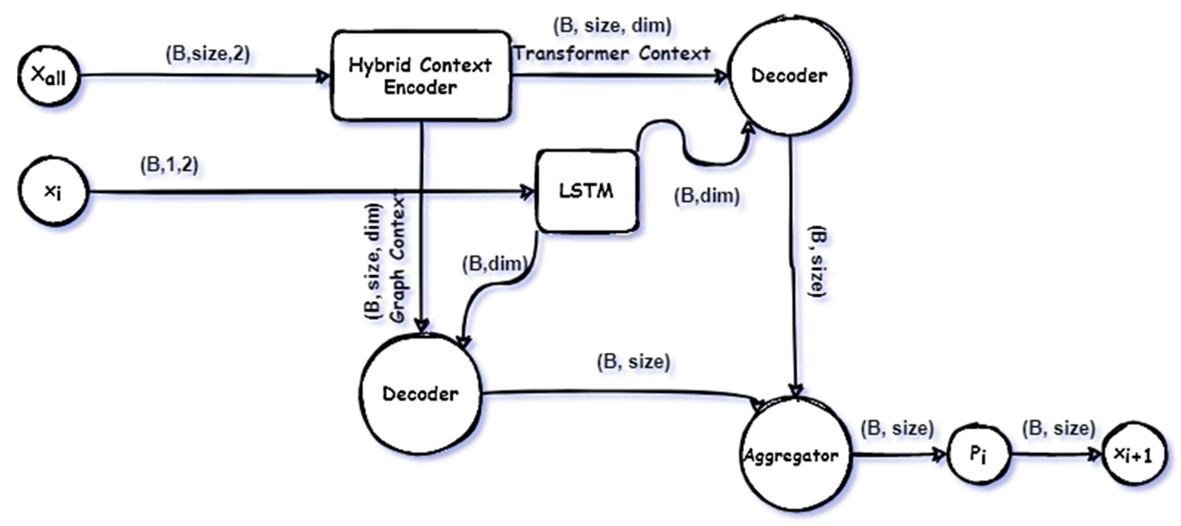
3. Model Architecture

As previously described in [1], the proposed model is a variation of the pointer networks [15]. Compared with GPN, the proposed model has two extra components: a hybrid context encoder and a multi attention decoder. The hybrid encoder is primarily composed of the transformer’s encoder and the graph encoder; these encoders encode the feature vector before passing it to the attention decoder layer. Therefore, there are two decoders at the decoding stage, one for the transformer context and one for the graph context. Finally, the output attention vectors from the two decoders are aggregated before selecting the next node in the tour. We will discuss the model architecture briefly in the next section. The proposed HPN is shown in Figure 1.

Which combining a hybrid context encoder with a multi-attention decoder. X_all is a tensor, which contains all cities’ features and x_i contains the currently selected city.

3.1. Hybrid Encoder

As illustrated in Figure 2. The encoder consists of:

Which consists of Transformer’s encoder and Graph embedding layer as a hybrid context encoder and the point encoder.

• Hybrid context encoder, the function of the hybrid context encoder is to encode the Feature vector $x=\left[x_1,x_2,\mathrm{e},\mathrm{l}\right]$ into two contextual vectors. Where $x_1$, $x_2$, $\mathrm{e}$ and $\mathrm{l}$ are the coordinates, entrance time and exit time for each point, respectively.
• Point encoder, which encodes the currently selected city using LSTM.

For the Hybrid context encoder, the first type of encoder used is a standard transformer encoder with multi-head attention:

$$H^{enc}=H^{l=L^{enc} }\in R^{n\times d}$$

(2)

where

$$H^l=softmax\left(\frac{Q^l{K}^{l^T}}{\sqrt{d}}\right)V^l \in R^{n\times d}$$

(3)

$$Q^l=H^l{W}_Q^L \in R^{n\times d}, W_Q^l \in R^{d\times d}$$

(4)

$$K^l=H^l{W}_K^L \in R^{n\times d}, W_K^l \in R^{d\times d}$$

(5)

$$V^l=H^l{W}_V^L \in R^{n\times d}, W_V^l \in R^{d\times d}$$

(6)

where $W_Q^L$, $W_K^L$ and $W_V^L$ are learnable parameters and $L$ denotes the number of layer for self-attention, $H^{enc}$ is a matrix containing the encoded nodes, $Q^l,K^l$ and $V^l$ are a query, key and value of the self-attention, respectively. Figure 3 illustrates the flow of the Data inside the Transformer encoder.

The second encoder type is a graph embedding layer, which encodes the Feature vector into a high dimensional vector. The graph is complete since we are just addressing symmetric TWTSP. Therefore, the graph embedding layer may be expressed as follows:

$$X^l=\gamma X^{l-1}{W}_g+\left(1-\gamma \right){\phi }_{\theta }\left(\frac{X^{l-1}}{\left|N\left(i\right)\right|}\right)$$

(7)

where $X^l \in R^{N\times d_l}, and {\phi }_{\theta }:R^{N\times d_{l-1} }\to R^{N\times d_l}$ is the aggregation function, $\gamma$ is a trainable parameter, $W_g\in R^{d_{l-1}\times d_l}$ is trainable weight matrix and $N\left(i\right)$ the adjacency matrix of node $i$. In this context $L$ denotes the number of layers used, $N$ denotes the number of cities and $d_l$ denotes the hidden dimension of the L-th layer.

For the point encoder which encodes the features vector $x_i$ of the current selected city $i$, each features vector is embedded into a higher dimensional vector ${\widehat{x}}_i\in R^d$, where $d$ is the hidden dimension. The vector ${\widehat{x}}_i$ for the current city $i$ is then encoded by an LSTM. $x_i^h$ is the hidden variable of the LSTM.

3.2. Multi-Decoder

The decoder is built on a pointer network’s attention mechanism and outputs the pointer vector $u_i$, which is then sent through a Softmax layer to generate a distribution over the following candidate cities. The following is the formulation of the attention mechanism and the pointer vector:

$$u_i^{(j)}=\{\begin{array}{c} V^T.\tanh \left(W_r{r}_j+W_{q}q\right) if j\ne \sigma \left(k\right), \forall k<j,\\ -\infty otherwise,\end{array}$$

(8)

where $u_i^{ (j)}$ considered as the jth element of the vector $u_i^{ }$, $W_r and W_q$ are trainable parameters, q is the query vector from the hidden state of the LSTM, $r_i$ is a reference vector containing the contextual information from all cities.

To illustrate the model operations in Figure 1, we feed the network a tensor of input nodes; in this problem the input nodes contain four features as previously illustrated so the input dimension will be (batch-size, problem-size, number-of-feature). We will feed these nodes into the hybrid context and will get two contextual vectors, one from the transformer’s encoder and the other from the graph encoder. Then, for the first decoding stamp, we feed to the pointer encoder the placeholder for learning the best possible location to start the decoding. Finally, we feed to our decoder, which is a simple attention layer of the contextual vectors with the hidden states from the pointer encoder and aggerate the two-attention vectors using the sum operation. For clarity, we use two decoders, layer one for the graph’s context vector and the other for the transformer’s context vector.

To this end, we incorporate the model with a graph embedding encoder beside the transformer’s encoder as a hybrid context encoder with an additional decoder layer. The model is then trained using the REINFORCE gradient estimator with a greedy rollout baseline [17].

4. Experimental Work

In this section, we discuss the details of the training and testing of the proposed model. Pytorch 1.7.0 is used to implement our model in

Table 2. Hyperparameters used for training.

Parameter	Value	Parameter	Value
Graph Embedding layer	3	Learning rate	1 × 10−4
Transformer Encoder	6	Batch size	512
Feed-forward dim	512	Training steps	2500
Optimizer	Adam	Tanh clipping	10
Epochs	100	Time Windows Expectation	1

, and summarizes the hyperparameters used during training. All tests are carried out on Kaggle’s GPU P100 with 16 GB of RAM. The average one epoch time for TWTSP20, TWTSP50 and TWTSP100 are 10 Min, 30 Min and 75 Min, respectively.

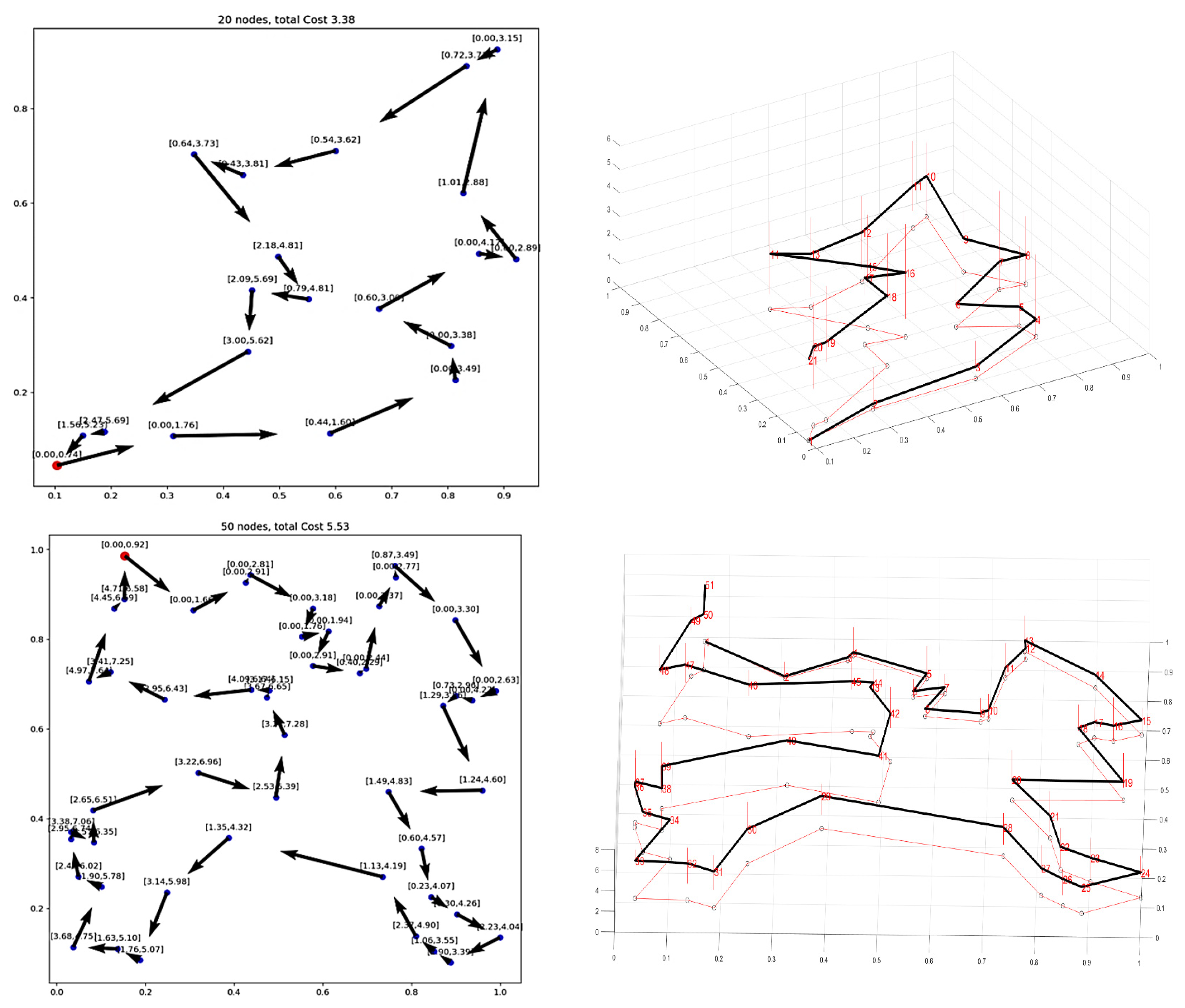
4.1. Simulated Dataset Generation

To generate training and testing data that has a feasible solution, we independently drew the coordinates of the nodes from a uniform distribution (i.e., $x1 and x2~uniform\left(0,1\right)$) [14]. Then, we solved the generated unconstrained instances using pre-trained HPN on the generated data. The HPN returned the time $t_i$ at the witch the salesman service node $i$. Therefore, for each node $i\in N_c$, we set $e_i=\max (t_i-{\widehat{e}}_i,0)$ and $l_i=t_i+{\widehat{l}}_i$, where ${\widehat{e}}_i~uniform\left(0,2\right)$ and ${\widehat{l}}_i~uniform(0,2)+1$. Therefore $e_i\le t_i\le l_i$, which means that a feasible solution in the training and test data always exist, and the expected time windows width is $1$ time unite. Finally, all the cities in the instance are randomly shuffled.

4.2. Reward Function

The reward function consists of two terms. One term is the penalty term:

$$p\left(t,l\right)={\displaystyle \sum }_{i=1}^{N_c}\max (l_i-t_i,0)$$

(9)

where this term will be added if the arriving time exceeds the leaving time. The other term is the total time cost of TWTSP solution. Consequently, the reward function is the total time cost of TWTSP solution plus the weighted penalty of missing one node $\beta \ast p\left(t,l\right)$, where $\beta$ is the penalty factor:

$$R=t_{n+1}+\beta \ast p\left(t,l\right)$$

(10)

We use $p\left(t,l\right)$ to calculate accuracy, which is the number of instances that are successfully solved. If $p\left(t,l\right)$> 0, there exists at least one city where the arrival time exceeds the upper bound of the time window, indicating that the solution is infeasible. In this experimental work we set the value of β equal to 10 as [14]. (

Table 3. Illustration of the simulated data generation.

#Algorithm 1 Data Simulation
1:   Input: pre-trained model for TSP, batch size B, problem size
2:   InputData = RandomInstance (B, size, 2)   #Random generate TSP points $\left(x1, x2\right)$ Features
3:   X = pre_trainedModel(InputData)    #Solve the points using pre-trained model, X is a tensor
4:  PrevCities = FirstCities               #contains the pre-trained model’s solution
5:   for t = 1,…, size do:
6:      current cities = X[t]    #Pick the current city
7:      cur_time ← EuclideanDistance(current_cities, PrevCities)  #Caluclate the Euc Distance
8:      X[:,t,2]   ← max(0,(cur_time − 2 ∗ RandomNumber)) #Entrance Time
9:      X[:,t,3]  ← cur_time + 2 ∗ RandomNumber + 1      #Leaving Time
10:   end for
11:  Shuffle(X)

) illustrates simulate data generation.

5. Results and Analysis

Findings recall that, in the context of the TSPTW problem, time features are added to the nodes’ coordinates such that each of the nodes $x_i$ is a quadruple $\left(x{1}_i,x{2}_i,e_i,l_i\right)$, where $\left(x{1}_i,x{2}_i\right)$ is a 2-D coordinate and $(e_i,l_i)$ are the entering and leaving time. To compare our results with OR-Tools, we used the Ant Colony Optimization (ACO) algorithm [18] and the graph pointer network (GPN) to solve the same TSPTW instances.

Table 4. Results for TSPTW 20-50-100. Obj: objective of TSPTW. Time: the running time of the algorithms. Feasible %: the percentage of instances that have feasible solutions by the algorithm. All results are averaged from 10K instances.

	TWTSP20			TWTSP50			TWTSP100
Method	Obj	Time	Feasible%	Obj	Time	Feasible%	Obj	Time	Feasible%
OR-Tools (Savings)	4.045	121 s	72.06%	6.251	1120 s	70.21%
ACO	4.655	204 s	62.10%	8.136	1493 s	61.52%
GPN Greedy	3.871	1 s	99.7%	5.95	3 s	99.97%	9.78	8 s	32.8%
HPN Greedy	3.867	1 s	100%	5.86	4 s	100%	8.32	12 s	99.97%

. shows the average trip cost for 10,000 TSPTW test instances. We employ the greedy search for prediction by simply taking the highest probability between the next candidates generated from our policy.

Even though all instances have feasible solutions based on our training setting, the algorithms will occasionally fail to discover a feasible solution. As an evaluation metric, we utilize the percentage of feasible solutions to represent this. To achieve fairness in comparison, we re-trained the GPN model using our settings.

Table 4 shows that our model can solve instances that has up to 100 nodes with a high accuracy ≈ 100%, whereas GPN can only solve up to 50 points. In the Obj column, we record the overall tour length costed by the tour as well as the sum of the time spent waiting for every point visited by our agent. The results show that our model outperforms all the paired approaches for TWTSP shown in Table 4. Furthermore, the proposed model has a better generalization for TWTSP100. Figure 4 shows HPN solutions for three TWTSP instances of 20.50 and 100 nodes size.

Figure 4 illustrates some examples of 3D plotting in which the z axis is the time dimension. Moreover, at each node we represent the time window by a line parallel to the z-axis and its start and end are the $e_i$ and $l_i$ respectively. In the figure, the tour line hits each bar at which the agent arrived to serve this point.

5.1. The Effect of Time Window

We intuitively understand that expanding the time windows from both sides makes the problem closer to be unconstrained TSP and may decrease tour cost. Furthermore, using representative data to train a machine learning model is important for building a generalized model. This fact sheds light on the importance of the expected width of the time window $E\left(W\right)$ used to simulate the training data. Recall that, in this research we set the expected width of the window equals 1. So, in this section we consider $E\left(W\right)$ is an indirect hyperparameter that needs fine tuning. Therefore, we conducted sensitivity analysis and investigates how the tour cost and feasibility vary as the width of the time window changes. We hypothesis that the larger the width of the expected time window the easier to find a solution. To test the above hypotheses, we generated four different datasets that have expected time window length of ½, 1, 2 and 4, respectively. Consequently, we trained four models each using one of the four datasets then we test each model using the four testing datasets. The performance of each model versus the testing dataset is shown in

Table 5. Total cost, time and feasible % metrics of the trained models versus the testing dataset generated using different expected time window width.

	NET1 (E(WT)) = ½			NET2 (E(WT)) = 1			NET3 (E(WT)) = 2			NET4 (E(WT)) = 4
	Cost	Wait	Acc	Cost	Wait	Acc	Cost	Wait	Acc	Cost	Wait	Acc
$E\left(W\right)$ = ½ e~2 ∗ uniform (0,1) L~2 ∗ uniform (0,1) + ½	3.89	0.003	99.99%	3.89	0.002	99.8	3.90	0.003	99.62%	4.2	0.001	85.5%
$E\left(W\right)$ = 1 e~2 ∗ uniform (0,1) L~2 ∗ uniform (0,1) +1	3.897	0.004	100%	3.88	0.002	100%	3.875	0.002	100%	4.04	0.008	99.51%
$E\left(W\right)$ = 2 e~2 ∗ uniform (0,1) L~2 ∗ uniform (0,1) + 2	4.14	0.009	100%	3.93	0.005	100%	3.858	0.001	100%	3.91	0.003	100%
$E\left(W\right)$ = 4 e~2 ∗ uniform (0,1) L~2 ∗ uniform (0,1) + 4	4.67	0.0113	100%	4.39	0.013	100%	3.985	0.009	100%	3.836	0.0008	100%

which records the average over 10,000 instances.

Table 5 shows that, as expected, increasing the window size of the training and testing makes it easier for the model to determine a good policy that yields tours with good cost as illustrated by the table above.

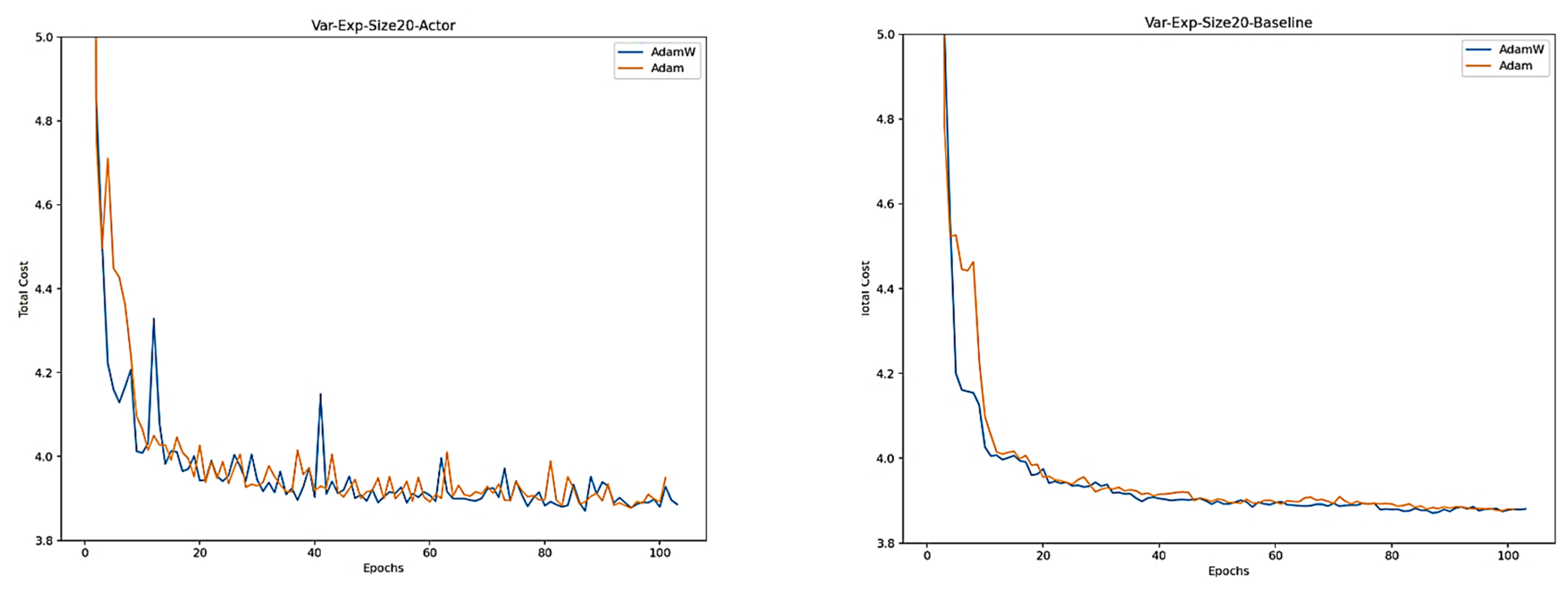
5.2. Variable Time Window

Table 5 also shows that, training a model with data that has a particular $E\left(W\right)$ and testing with data that has a different $E\left(W\right)$ increases the average trip cost which is an unwanted effect. So, the size of time windows is an important design choice; perhaps we can make it an indirect hyperparameter. In this section, we will illustrate the effect of variable expected time windows on the model performance using Adam and Adam W optimizers.

As proposed by Ilya Loshchilov [19], the weight decay is inherently tied to the learning rate in the Adam optimizer’s common weight decay implementation. This means that when improving the learning rate, you must also discover a new optimal weight decay for each learning rate you test. The weight decay is decoupled from the optimization stage by the AdamW optimizer. This indicates that the weight decay and learning rate may be adjusted independently, and that altering the learning rate has no effect on the ideal weight decay. As a result of this modification, generalization performance has significantly improved.

So, we generated a TWTSP20 dataset that has variable expected time windows ranging from 1 to 5. Then we created two instances of our proposed model and train each one using different optimizers (i.e., Adam and AdamW). Figure 5 illustrates the performance for these two experiments.

We could see that there is a large spike on the beginning of the training for Adam, but that’s not affecting the total performance; both optimizer’s results are very close and we can say that Adam W is smoother than Adam. However, there is no difference between both of them on the final result.

Table 6. Evaluation performance for both Adam and Adam W, Cost indicates to the total cost for the tour which is the total tour length plus the total time wait.

Type of Data	NET1 AdamW			NET2 Adam
Data-Variable-Exp	Cost	Acc	Wait	Cost	Acc	Wait
$E\left(W\right)$ = ½	3.875	100%	0.0037	3.877	100%	0.003
$E\left(W\right)$ = 1	3.89	99.14%	0.0022	3.90	98.76%	0.0019
$E\left(W\right)$ = 2	3.885	99.89%	0.002	3.887	99.97%	0.0019
$E\left(W\right)$ = 4	3.88	99.98%	0.003	3.876	100%	0.003
$E\left(W\right)$ = 8	3.875	100%	0.005	3.887	100%	0.007
$E\left(W\right)$ = 16	4.086	100%	0.008	3.99	100%	0.03

shows the evaluation performance for TWTSP20 trained on variable expected time windows, one with Adam and the other with Adam W.

Table 6 shows that the two trained models give good results when tested using $E\left(W\right)$ outside the range used in the training dataset, which means that using training data that has variable $E\left(W\right)$ results in a better generalized model.

6. Conclusions

In this paper, we developed an RL-based model to solve the traveling salesman problem with time windows. The developed model is based on using different encoders and decoders to be able to better model the joint distribution between the problem features and the solution. We compared the proposed model with the GPN and showed that our model yields better trips and can solve larger instances. Our model is still not capable of generalizing two very large problem instances i.e., TWTSP500 and TWTSP1000. We will let this work into our future direction.

Future research could lead to the development of multi-objective optimization models that consider multiple objectives such as customer satisfaction, tour duration, and solution time, as well as various constraints such as road traffic, municipality ordinances and codes, and labor standards.

References

1. Stohy, A.; Abdelhakam, H.-T.; Ali, S.; Elhenawy, M.; Hassan, A.A.; Masoud, M.; Glaser, S.; Rakotonirainy, A. Hybrid Pointer Networks for Traveling Salesman Problems Optimization. arXiv 2021, arXiv:2110.03104. [Google Scholar]
2. Carlton, W.B.; Barnes, J.W. Solving the Traveling-Salesman Problem with Time Windows Using Tabu Search. IIE Trans. 1996, 28, 617–629. [Google Scholar] [CrossRef]
3. Gendreau, M.; Hertz, A.; Laporte, G.; Stan, M. A Generalized Insertion Heuristic for the Traveling Salesman Problem with Time Windows. Oper. Res. 1998, 46, 330–335. [Google Scholar] [CrossRef]
4. Gendreau, M.; Hertz, A.; Laporte, G. New Insertion and Postoptimization Procedures for the Traveling Salesman Problem. Oper. Res. 1992, 40, 1086–1094. [Google Scholar] [CrossRef]
5. Calvo, R.W. A New Heuristic for the Traveling Salesman Problem with Time Windows. Transp. Sci. 2000, 34, 113–124. [Google Scholar] [CrossRef]
6. Ohlmann, J.W.; Thomas, B.W. A compressed-annealing heuristic for the traveling salesman problem with time windows. Informs J. Comput. 2007, 19, 80–90. [Google Scholar] [CrossRef] [Green Version]
7. Kirkpatrick, S.; Gelatt, C.D.; Vecchi, M.P. Optimization by simulated annealing. Science 1983, 220, 671–680. [Google Scholar] [CrossRef] [PubMed]
8. Savelsbergh, M.W. Local search in routing problems with time windows. Ann. Oper. Res. 1985, 4, 285–305. [Google Scholar] [CrossRef] [Green Version]
9. Christofides, N.; Mingozzi, A.; Toth, P. State-space relaxation procedures for the computation of bounds to routing problems. Networks 1981, 11, 145–164. [Google Scholar] [CrossRef]
10. Baker, E.K. Technical Note—An Exact Algorithm for the Time-Constrained Traveling Salesman Problem. Oper. Res. 1983, 31, 938–945. [Google Scholar] [CrossRef] [Green Version]
11. Dumas, Y.; Desrosiers, J.; Gelinas, E.; Solomon, M.M. An Optimal Algorithm for the Traveling Salesman Problem with Time Windows. Oper. Res. 1995, 43, 367–371. [Google Scholar] [CrossRef] [Green Version]
12. Pesant, G.; Gendreau, M.; Potvin, J.-Y.; Rousseau, J.-M. An Exact Constraint Logic Programming Algorithm for the Traveling Salesman Problem with Time Windows. Transp. Sci. 1998, 32, 12–29. [Google Scholar] [CrossRef] [Green Version]
13. Pesant, G.; Gendreau, M.; Potvin, J.-Y.; Rousseau, J.-M. On the flexibility of constraint programming models: From single to multiple time windows for the traveling salesman problem. Eur. J. Oper. Res. 1999, 117, 253–263. [Google Scholar] [CrossRef]
14. Ma, Q.; Ge, S.; He, D.; Thaker, D.; Drori, I. Combinatorial optimization by graph pointer networks and hierarchical reinforcement learning. arXiv 2019, arXiv:1911.04936. [Google Scholar]
15. Vinyals, O.; Fortunato, M.; Jaitly, N. Pointer networks. arXiv 2015, arXiv:1506.03134. [Google Scholar]
16. Stohy, A. Solving Traveling Salesman Problem with Time Windows Using Hybrid Pointer Networks with Time Features. 2021. Available online: https://www.researchgate.net/publication/355142062_Hybrid_Pointer_Networks_for_Traveling_Salesman_Problems_Optimization (accessed on 17 November 2021).
17. Kool, W.; Van Hoof, H.; Welling, M. Attention, learn to solve routing problems! arXiv 2018, arXiv:1803.08475. [Google Scholar]
18. Cheng, C.-B.; Mao, C.-P. A modified ant colony system for solving the travelling salesman problem with time windows. Math. Comput. Model. 2007, 46, 1225–1235. [Google Scholar] [CrossRef]
19. Loshchilov, I.; Hutter, F. Decoupled weight decay regularization. arXiv 2017, arXiv:1711.05101. [Google Scholar]
Figure 1. Architecture of HPN.
Sustainability 13 12906 g001
Figure 2. Hybrid encoder.
Sustainability 13 12906 g002
Figure 3. Transformer’s Encoder used to encode the Feature Vector.
Sustainability 13 12906 g003
Figure 4. Sample tours TWTSP20, TWTSP50 and TWTSP100 solved by HPN the cost included the total tour distance plus any time wait each point labeled with its time window (Entrance, Leaving) on 2D space on the left. On the right, plotting the x and y axes for the coordinates of the point and the z axis for the available time window for that point.
Sustainability 13 12906 g004aSustainability 13 12906 g004b
Figure 5. Training performance for TWTSP20 with variable expected time window where the left panel shows the Actor performance, and the right panel shows the critic performance.
Sustainability 13 12906 g005