Green Credit Financing Equilibrium under Government Subsidy and Supply Uncertainty

Abstract

In this paper, we study the green credit financing equilibrium in a green supply chain (GSC) with government subsidy and supply uncertainty. The GSC system is composed of one manufacturer, two retailers, one bank, and the government. The manufacturer is subject to both supply uncertainty and limited capital. The manufacturer invests in the R&D of green products and borrows loans from the bank. The government subsidizes banks to encourage banks to provide loans to manufacturers with lower interest rates, which is termed “green credit financing”. The two retailers decide their order quantities with horizontal competition or horizontal cooperation. We first developed a Stackelberg model to investigate the green credit financing equilibriums (i.e., the interest rate of the bank, the manufacturer’s product green degree and wholesale price, and the retailers’ order quantity) under horizontal competition and horizontal cooperation, respectively. Subsequently, we analyzed how the subsidy interest rate, supply uncertainty, and supply correlation affect financing decisions regarding equilibrium green credit. We found that a high subsidy interest rate leads to a low interest rate of bank and the manufacturer can set a high level of green product and high wholesale price, while the retailers can set a high order quantity. Finally, we compared the green credit financing equilibriums under horizontal competition with those under horizontal cooperation using numerical and analytical methods. We found that, in general, the optimal decisions and profits of bank and SC members, consumer surplus, and social welfare under horizontal competition are higher than those under horizontal cooperation. The findings in this research could provide valuable insights for the management of capital-constrained GSCs with government subsidies and supply uncertainty in a competing market.

1. Introduction

To achieve the coordinated development of economy, society, and environment, the government adopts many measures to encourage firms to manufacture green products. A green product refers to a sustainable product designed to cause minimum environmental pollution during its total life cycle. With the increasing awareness of customers regarding environmental protection, green products are becoming increasingly favored by consumers. Manufacturers are willing to invest in the R&D of green product to improve brand loyalty, a positive public image, and access to new markets. Green products are also essential to society for preventing overuse of resources and protecting the environment. However, the R&D of green products requires additional investment and much capital (https://www.feedough.com/green-product/, accessed on 1 November 2021). Due to limited capital, manufacturers are often cash-strapped and need to borrow money from banks, which is termed green credit financing (GCF) (An et al. [1]).

Green credit financing (GCF), which is often used in industries, has attracted the attention of researchers. For example, Huang et al. [2], An et al. [1], Ling et al. [3], and Deng et al. [4] analyzed the effect of green credit on pollution-intensive firms’ investments in green technological innovation, without examining the impact of supply uncertainty on GCF under horizontal competition and horizontal cooperation. Our study fills this gap by considering downstream firms facing an uncertain correlated yield process from capital-constrained upstream enterprises.

Motivated by the analysis of GCF from both industrial and academic research, this study investigates GCF-given government subsidy and supply uncertainty in a green supply chain (GSC). The GSC system consists of one manufacturer, two retailers, one bank, and the government. The manufacturer is subject to limited capital and supply uncertainty. For example, BYD Co., Ltd., an electric car manufacturer in China, faces high R&D costs due to new technology and uncertain yield process (supply uncertainty). Subsequently, its retailers (e.g., 4S dealership offering sales, service, spare parts, and survey feedback) face an uncertain correlated yield process from BYD (i.e., supply correlation) (Jung [5]). BYD can obtain loans from banks to address capital shortage issues (https://www.byd.com/cn/Investor/InvestorAnnals.html, accessed on 1 November 2021). To encourage the manufacturer to invest in green products (e.g., electric cars), the government subsidizes the bank in order for manufacturers to obtain a lower-interest loan (Huang et al. [2]; An et al. [1]). In this research, we consider two retailers with two types of order quantities: retailers that can form an alliance and those that cannot. Namely, the two retailers choose their order quantities jointly through coalition (i.e., horizontal cooperation) or decide on their quantities independently (i.e., horizontal competition).

Based on the discussion above, we identified the following research questions:

• What is the green credit financing equilibrium under horizontal competition and horizontal cooperation, respectively?
• How do subsidy interest rate, supply uncertainty, and supply correlation affect the optimal green credit equilibrium?
• How do retailers’ order modes (i.e., order quantity under horizontal competition or cooperation) affect the optimal decisions and profits of the bank and GSC members, consumer surplus, and social welfare?

To address these questions, we built a Stackelberg model to explore GCF under government subsidy and supply uncertainty. Using backward induction, we identified the equilibrium GCF under horizontal competition and horizontal cooperation, respectively.

The main focus and findings of the research and the corresponding implications are summarized below.

• We examined the effect of key parameters, including the subsidy interest rate, supply uncertainty, and supply correlation, on the equilibrium GCF decisions. We found that a higher subsidy rate (low supply correlation, low supply uncertainty) corresponds to a lower bank interest rate, a higher product green degree, a higher wholesale price, and higher order quantities. This suggests that the subsidy rate and supply correlation affect the bank and GSC members in opposite directions, while supply correlation and supply uncertainty affect the bank and GSC members in the same direction.
• By analyzing the retailers’ order modes choice (i.e., order quantity under horizontal cooperation or competition), we found that the manufacturer, the bank, and retailers gain more profits in Case I (i.e., the two retailers with horizontal cooperation) than in Case II (i.e., the two retailers with horizontal competition). This suggests that retailers who decide their order quantities independently can gain more profit than those who decide on the order quantity jointly with the alliance.
• Finally, we compared consumer surplus and welfare between the horizontal competition and the horizontal cooperation settings. We found that consumer surplus and social welfare in Case I were higher than those in Case II.

The remainder of this paper is organized as follows. In Section 2, we review and discuss related literature. Section 3 presents the research framework. The green credit financing equilibrium decisions are presented in Section 4. The optimal operational decisions and profits of bank and SC members, consumer surplus, and social welfare are compared through a numerical study in Section 5. Section 6 summarizes the conclusions and contributions and gives future research directions. All proofs can be found in Appendix A.

2. Literature Review

Two streams of literature most relevant to our work were: GCF in a capital constrained GSC and government subsidy in a GSC. They are discussed below.

2.1. GCF in a Capital-Constrained GSC

Researchers have studied the financing strategy choices between bank credit financing (i.e., loan from banks) and trade credit financing (i.e., borrowing from cooperative SC members) in SCs with one upstream and one downstream firm. Tang and Yang [6] investigated the effect of power structure on supply chain financing decisions. Shen et al. [7] explored how risk preference affects supply chain financing decisions under different supply chain structures. Deng et al. [8] further investigated the competing upstream suppliers’ financing strategy choice among trade credit financing and bank credit financing. Similarly, Lu and Wu [9], Jing et al. [10], Cai et al. [11], and Chen [12] investigated the capital-constrained downstream enterprise financing strategy under different SC operational settings.

Recently, Gao et al. [13] investigated the value of online peer-to-peer (P2P) lending platforms on a capital constrained supply chain’s financing decision. Jin et al. [14] explored a capital constrained supply chain member and they decided whether to collaborate with each other on the financing decision. Kang et al. [15] discussed the value of green credit strategy and how to incentivize the downstream manufacturer to cooperate with the upstream supplier in investing on pollution abatement. Ding and Wan [16], Zou et al. [17], and Yuan et al. [18] investigated the impact of supply uncertainty on the financing and operational decisions of SCs. Other researchers have focused on green credit financing. An et al. [1], Ling et al. [3], and Fang and Xu [19] found that green credit financing is an effective tool to promote sustainable business development. Huang et al. [2] and Deng et al. [4] further studied the green credit financing strategy by considering government subsidies. In contrast to the extant studies, we investigated the impact of supply uncertainty on GCF.

2.2. Government Subsidy in a GSC

Governments often encourage enterprises to invest in green innovation by offering subsidies. Huang et al. [20] explored how green loans and government subsidies jointly affect firms’ green efforts. Li et al. [21] found that government subsidies can incentivize upstream and downstream firms to cooperate in green endeavors. Bian and Zhao [22] and Yang et al. [23] investigated the impact of subsidies on green innovation under competition. Bai et al. [24] discussed the value of the subsidy strategy for green innovation. Sun et al. [25] investigated the upstream SC member’s green investment strategies through evolutionary game theory. Zhang et al. [26] and Li et al. [27] further discussed the impact of government subsidies on green technology innovation decisions for vehicles. Some researchers examined the investment of the R&D on a green product in a GSC. Dong et al. [28] investigated the capital constrained supply chain members’ investment strategy on the R&D of a green product. Jung and Feng [29] examined the effect of government subsidy on green technology development in an evolving industry. Guo et al. [30] further examined the issue of green product R&D under competition through the case study of the fashion apparel industry. Finally, Ren et al. [31] discussed the issue of green products selling on ecommerce platforms, but they did not consider the endogenous interest rate of banks, as we have done in our research.

In brief, our work differs from the literature by jointly considering government subsidies, the endogenous interest rate of the bank, supply uncertainty and correlation, and competition at market demand.

Table 1. Table of related literature vs. our work.

Authors	Supply Uncertainty	Supply Correlation	Green Innovation	Government Subsidy	Green Credit Financing	Endogenous Interest Rate of the Bank	Competition
This paper	√	√	√	√	√	√	√
An et al. [1]			√		√
Huang et al. [2]			√	√	√	√	√
Ling et al. [3]			√		√
Deng et al. [4]			√	√	√
Jung [5]	√	√					√
Tang and Yang [6]			√		√
Shen et al. [7]			√		√		√
Lu and Wu [9]			√		√
Jing et al. [10]			√		√
Cai et al. [11]			√		√
Chen [12]			√		√
Ding and Wan [16]			√	√	√
Zou et al. [17]	√		√		√	√
Yuan et al. [18]	√		√		√
Fang and Xu [19]	√		√		√	√
Huang et al. [20]			√	√	√
Li et al. [21]			√	√
Bian and Zhao [22]			√	√			√
Yang et al. [23]			√	√			√
Bai et al. [24]			√	√
Sun et al. [25]			√	√
Zhang et al. [26]			√	√
Li et al. [27]			√	√
Dong et al. [28]			√
Jung and Feng [29]			√	√
Guo et al. [30]			√				√

contrasts our research with previous studies.

3. Research Framework

We focused on a GSC system consisting of one manufacturer, two retailers, one bank, and the government. The manufacturer was subject to both supply uncertainty and limited capital. We developed a Stackelberg game model to address the green credit financing equilibrium problem for the setting described below.

3.1. Green Credit Financing with Government Subsidy

We considered a linear demand function. The reverse demand function under competition can be characterized as $P=a+\lambda e-\left(Q_1+Q_2\right)$. Parameters $P$ and $a$ represent the product’s selling price and potential market demand, respectively. Parameter $e$ denotes the manufacturer’s green level of the product, and the corresponding cost is $\frac{1}{2}k{e}^2$. To focus on the green credit financing (GCF) strategy, we only considered the green effort cost $\frac{1}{2}k{e}^2$. We normalized the manufacturer’s product cost per unit and set the distribution cost to zero while assuming the manufacturer’s initial capital was zero. The manufacturer borrows $\frac{1}{2}k{e}^2$ amount from the bank with an interest rate, $r$. The bank can receive a total of $\frac{1}{2}k{e}^2\left(r+\tau \right)$ with $\frac{1}{2}k{e}^{2}r$ from the manufacturer and $\frac{1}{2}k{e}^2\tau$ from government subsidy. In our work, the interest rate of the bank was endogenous (Huang et al. [2]).

Respectively, $\lambda$ and $k$ denote the consumer’s green preference and cost coefficient for green product investment. $Q_1$ and $Q_2$ represent the selling quantities, corresponding to retailer 1 and retailer 2. Owing to the manufacturer’s yield process uncertainty, $Q_1=y_1{q}_1$ and $Q_2=y_2{q}_2$. $q_1$ and $q_2$ are the respective order quantity of retailers 1 and 2 from the manufacturer. We assumed that if $y_i\in \left(0,1\right]$ and $y_i~N\left({\mu }_y,{\sigma }_y^2\right)$, i = 1, 2. Let ${\delta }_y={\sigma }_y/{\mu }_y$ denote the degree of supply uncertainty. $\rho =\frac{Cov\left(y_1{y}_2\right)}{\sqrt{Var\left(y_1\right)Var\left(y_2\right)}}\in \left(0,1\right)$ represents the supply correlation.

3.2. The Sequences of Events

The SC members’ decision sequences were as follows:

(1)

The bank determines the interest rate.

(2)

The manufacturer concurrently determines the green level of the product and wholesale price.

(3)

The retailers decide order quantities independently (i.e., retailers with horizontal competition) or jointly through horizontal cooperation.

(4)

The manufacturer produces products and distributes them.

(5)

Supply-side uncertainty is realized.

Table 2. Parameters and variables.

Variables	Descriptions
$q_i^Z$	The retailer i’s order quantity under case $Z$; $Z=I, II$ (a decision variable);
$e^Z$	The manufacturer’s green level of product under case $Z$ (a decision variable);
$w^Z$	The manufacturer’s wholesale price under case $Z$ (a decision variable);
$r^Z$	The bank’s interest rate under case $Z$ (a decision variable);
$y_i$	Supply yield variability factor, $y_i\in \left(0,1\right)$, $y_i~N\left(\mu ,{\sigma }_y^2\right)$ (a random variable), $0<\mu \le 1$, ${\sigma }_y\in \left(0,\infty \right)$;
${\Pi }_{R_i}^Z$	The retailer i’s profit under case $Z$;
${\Pi }_B^Z$	The bank’s profit under case $Z$;
${\Pi }_M^Z$	The manufacturer’s profit under case $Z$;
$G^Z$	The total subsidy of government under case $Z$;
$C{S}^Z$	Consumer surplus under case $Z$;
$S{W}^Z$	Social welfare under case $Z$.
Parameters	Descriptions
$a$	Potential market size, $a>0$;
${\delta }_y$	Supply uncertainty, ${\delta }_y=\frac{{\sigma }_y}{\mu }$, and ${\delta }_y\in \left(0,\infty \right)$;
$\rho$	Supply correlation, and $\rho \in \left(0,1\right)$;
$\lambda$	Consumer’s green preference, $\lambda \in \left(0,1\right)$;
$k$	The investment cost coefficient of green technology, $k>0$.
Indices	Descriptions
Subscript	$M$ and B represent the manufacturer and the bank; $R_i$ represents retailer i;
Superscript	Case I represents the retailers with horizontal competiton; Case II represents the retailers with horizontal cooperation; * denotes the value is “optimal” or “equilibrium”.

summarizes the parameters and variables used in this research.

4. Green Credit Financing Equilibrium Decisions

In this section, we first provide green credit financing equilibrium operational decisions under horizontal competition (Case I) and horizontal cooperation (Case II). Then the profits of the bank and GSC member firms, total government subsidy, consumer surplus, and social welfare are discussed.

4.1. Green Credit Financing Equilibrium Decisions under Horizontal Competition (Case I)

In Case I, the two retailers engaged in horizontal competition. The two retailers decided their order quantities simultaneously and independently.

Thus, the two retailers’ optimization problems are expressed as follows:

$$\underset{q_1^I>0}{\max } {\Pi }_{R_1}^I=E\left\{\left[a+\lambda e^I-\left(y_1{q}_1^I+y_2{q}_2^I\right)\right]y_1{q}_1^I-w^I{y}_1{q}_1^I\right\}$$

(1)

$$\underset{q_2^I>0}{\max } {\Pi }_{R_2}^I=E\left\{\left[a+\lambda e^I-\left(y_1{q}_1^I+y_2{q}_2^I\right)\right]y_2{q}_2^I-w^I{y}_2{q}_2^I\right\}$$

(2)

The manufacturer’s optimization problem is

$$\underset{w^I>0}{\max } {\Pi }_M^I=E\left\{w^I\left(y_1{q}_1^I+y_2{q}_2^I\right)-\left(1+r^I\right)\frac{1}{2}k{\left(e^I\right)}^2\right\}$$

(3)

The bank’s optimization problem is

$$\underset{r^I>0}{\max } {\Pi }_B^I=\frac{1}{2}k{\left(e^I\right)}^2\left(r^I+\tau \right)$$

(4)

Solving Equations (1)–(4) using backward induction, we obtained equilibrium solutions, which are summarized in Proposition 1.

Proposition 1.

Given $k>\frac{{\lambda }^2}{\left[3+\left(2+\rho \right){\delta }_y^2\right]\left(1-\tau \right)}$, when the two retailers engage in horizontal Cournot competition (Case I), we have:

(1) 

The bank’s optimal interest rate is

$$r^{I*}=\frac{k\left(1-2\tau \right)\left[3+\left(2+\rho \right){\delta }_y^2\right]-{\lambda }^2}{k\left[3+\left(2+\rho \right){\delta }_y^2\right]}$$

(5)

(2) 

The manufacturer’s optimal product green degree and the wholesale price are

$$e^{I*}=\frac{\lambda a}{2\left\{k\left(1-\tau \right)\left[3+\left(2+\rho \right){\delta }_y^2\right]-{\lambda }^2\right\}}$$

(6)

$$w^{I*}=\frac{\left\{2k\left(1-\tau \right)\left[3+\left(2+\rho \right){\delta }_y^2\right]-{\lambda }^2\right\}a}{4\left\{k\left(1-\tau \right)\left[3+\left(2+\rho \right){\delta }_y^2\right]-{\lambda }^2\right\}}$$

(7)

(3) 

The two retailers’ optimal order quantities are

$$q_1^{I*}=q_2^{I*}=\frac{\left\{2k\left(1-\tau \right)\left[3+\left(2+\rho \right){\delta }_y^2\right]-{\lambda }^2\right\}a}{4{\mu }_y\left[3+\left(2+\rho \right){\delta }_y^2\right]\left\{k\left(1-\tau \right)\left[3+\left(2+\rho \right){\delta }_y^2\right]-{\lambda }^2\right\}}$$

(8)

Proposition 1 provides the equilibrium decisions of the bank and SC members when two retailers engage in horizontal competition. Proposition 1 also shows that the equilibrium decisions ($r^{I*}$, $w^{I*}$, $w^{I*}$, $q_1^{I*},$ and $q_2^{I*}$) depend on the government subsidy interest rate ($\tau$), supply uncertainty (${\delta }_y$), and supply correlation ($\rho$). Proposition 1 suggests that, when the bank makes the interest rate decision, the manufacture makes green product degree decisions and wholesale price decisions, and the retailers make their order quantity decisions, they all need to take the subsidy rate, supply correlation, and supply uncertainty into consideration.

Next, we discuss how $\tau$, $\rho ,$ and ${\delta }_y$ affect $r^{I*}$, $w^{I*}$, $w^{I*}$, $q_1^{I*}$, and $q_2^{I*}$, respectively, and summarize the main results in Corollaries 1–3.

Corollary 1.

The impacts of the government subsidy interest rate ($\tau$) on the equilibrium decisions under horizontal Cournot competition (Case I) are as follows:

(1) 

The optimal interest rate ($r^{I*}$) decreases with$\tau$(i.e.,$\frac{\partial r^{I*}}{\partial \tau }<0$);

(2) 

The optimal product green level ($e^{I*}$) increases with$\tau$(i.e.,$\frac{\partial e^{I*}}{\partial \tau }>0$);

(3) 

The optimal wholesale price ($w^{I*}$) increases with$\tau$(i.e.,$\frac{\partial w^{I*}}{\partial \tau }>0$);

(4) 

The optimal order quantities ($q_1^{I*}$and$q_2^{I*}$) increase with$\tau$(i.e.,$\frac{\partial q_1^{I*}}{\partial \tau }=\frac{\partial q_2^{I*}}{\partial \tau }>0$).

Corollary 1 states that a higher $\tau$ corresponds to a lower $r^{I*}$ and a higher $e^{I*}$ ($w^{I*}$, $q_1^{I*}$, and $q_2^{I*}$). This is because, if the government provides a higher $\tau$ to the bank, the bank will set a lower $r^{I*}$. With a lower financing cost, the manufacturer can set a higher $e^{I*}$. High $e^{I*}$ corresponds to high investment cost in green products. Thus, the manufacturer sets high $w^{I*}$. Higher $e^{I*}$ leads to higher demand; thus, the two retailers will set higher $q_1^{I*}$ and $q_2^{I*}$.

Corollary 2.

The impact of supply correlation ($\rho$) on the equilibrium decisions under horizontal Cournot competition (Case I) is expressed as follows:

(1) 

The optimal interest rate ($r^{I*}$) increases with$\rho$(i.e.,$\frac{\partial r^{I*}}{\partial \rho }>0$);

(2) 

The optimal product green level ($e^{I*}$) decreases with$\rho$(i.e.,$\frac{\partial e^{I*}}{\partial \rho }<0$);

(3) 

The optimal wholesale price ($w^{I*}$) decreases with$\rho$(i.e.,$\frac{\partial w^{I*}}{\partial \rho }<0$);

(4) 

The optimal order quantities ($q_1^{I*}$and$q_2^{I*}$) decrease with$\rho$(i.e.,$\frac{\partial q_1^I}{\partial \rho }=\frac{\partial q_2^I}{\partial \rho }<0$).

Corollary 3.

The impact of supply uncertainty (${\delta }_y$) on the equilibrium decisions under horizontal Cournot competition (Case I) is expressed as follows:

(1) 

The optimal interest rate ($r^{I*}$) increases with${\delta }_y$(i.e.,$\frac{\partial r^{I*}}{\partial {\delta }_y}>0$);

(2) 

The optimal product green level ($e^{I*}$) decreases with${\delta }_y$(i.e.,$\frac{\partial e^{I*}}{\partial {\delta }_y}<0$);

(3) 

The optimal wholesale price ($w^{I*}$) decreases with${\delta }_y$(i.e.,$\frac{\partial w^{I*}}{\partial {\delta }_y}<0$);

(4) 

The optimal order quantities ($q_1^{I*}$and$q_2^{I*}$) decrease with${\delta }_y$(i.e.,$\frac{\partial q_1^I}{\partial {\delta }_y}=\frac{\partial q_2^I}{\partial {\delta }_y}<0$).

Corollaries 2–3 show that $\rho$ and ${\delta }_y$ affect the equilibrium decisions in the same direction. A high $\rho$ indicates a high degree of competition between the two retailers and leads to lower $q_1^{I*}$ and $q_2^{I*}$. Thus, the manufacturer sets a low $w^{I*}$ and $e^{I*}$. Accordingly, the bank sets a high $r^{I*}$.

From Proposition 1, we can then obtain Proposition 2, below.

Proposition 2.

Given $k>\frac{{\lambda }^2}{\left[3+\left(2+\rho \right){\delta }_y^2\right]\left(1-\tau \right)}$, when the two retailers engage in horizontal Cournot competition (Case I), we have:

(1) 

The manufacturer’s profit is

$${\Pi }_M^{I*}=\frac{\left\{2k\left(1-\tau \right)\left[3+\left(2+\rho \right){\delta }_y^2\right]-{\lambda }^2\right\}{a}^2}{4\left[3+\left(2+\rho \right){\delta }_y^2\right]\left\{k\left(1-\tau \right)\left[3+\left(2+\rho \right){\delta }_y^2\right]-{\lambda }^2\right\}}$$

(9)

(2) 

The retailers’ profits are

$${\Pi }_{R_1}^{I*}={\Pi }_{R_2}^{I*}=\frac{\left(1+{\delta }_y^2\right){\left\{2k\left(1-\tau \right)\left[3+\left(2+\rho \right){\delta }_y^2\right]-{\lambda }^2\right\}}^2{a}^2}{16{\left[3+\left(2+\rho \right){\delta }_y^2\right]}^2{\left\{k\left(1-\tau \right)\left[3+\left(2+\rho \right){\delta }_y^2\right]-{\lambda }^2\right\}}^2}$$

(10)

(3) 

The bank’s profit is

$${\Pi }_B^{I*}=\frac{\left\{k\left[3+\left(2+\rho \right){\delta }_y^2\right]\left(1-\tau \right)-{\lambda }^2\right\}{\lambda }^2{a}^2}{8\left[3+\left(2+\rho \right){\delta }_y^2\right]{\left\{k\left[3+\left(2+\rho \right){\delta }_y^2\right]\left(1-\tau \right)-{\lambda }^2\right\}}^2}$$

(11)

(4) 

The total subsidy of government is

$$G^{I*}=\frac{k{\lambda }^2{a}^2\tau }{8{\left\{k\left[3+\left(2+\rho \right){\delta }_y^2\right]\left(1-\tau \right)-{\lambda }^2\right\}}^2}$$

(12)

(5) 

Consumer surplus and social welfare are

$$C{S}^{I*}=\frac{1}{2}E\left[{\left(y_1{q}_1^{I*}+y_2{q}_2^{I*}\right)}^2\right]=\frac{\left[2+\left(1+\rho \right){\delta }_y^2\right]{\left\{2k\left(1-\tau \right)\left[3+\left(2+\rho \right){\delta }_y^2\right]-{\lambda }^2\right\}}^2{a}^2}{16{\left[3+\left(2+\rho \right){\delta }_y^2\right]}^2{\left\{k\left(1-\tau \right)\left[3+\left(2+\rho \right){\delta }_y^2\right]-{\lambda }^2\right\}}^2}$$

(13)

$$S{W}^{I*}={\Pi }_M^{I*}+{\Pi }_{R_1}^{I*}+{\Pi }_{R_2}^{I*}+{\Pi }_B^{I*}+C{S}^{I*}-G^{I*}$$

(14)

Proposition 2 gives the corresponding bank’s profit, SC members’ profits, total government subsidy, consumer surplus, and social welfare.

4.2. Green Credit Financing Equilibrium under Horizontal Cooperation (Case II)

When the two retailers form an alliance, i.e., the two retailers formulate horizontal cooperation (Case II), the order quantity of the two retailers are decided jointly.

Thus, the joint optimization problem is expressed as follows:

$$\underset{q_1^{II}>0,q_2^{II}>0}{\max } {\Pi }_{alliance}^{II}={\Pi }_{R_1}^{II}+{\Pi }_{R_2}^{II}=E\left\{\left[a+\lambda e^{II}-w^{II}-\left(y_1{q}_1^{II}+y_2{q}_2^{II}\right)\right]\left(y_1{q}_1^{II}+y_2{q}_2^{II}\right)\right\}$$

(15)

The manufacturer’s optimization problem is

$$\underset{w^{II}>0}{\max } {\Pi }_M^{II}=E\left\{w^{II}\left(y_1{q}_1^{II}+y_2{q}_2^{II}\right)-\left(1+r^{II}\right)\frac{1}{2}k{\left(e^{II}\right)}^2\right\}$$

(16)

The bank’s optimization problem is

$$\underset{r^{II}>0}{\max } {\Pi }_B^{II}=\frac{1}{2}k{\left(e^{II}\right)}^2\left(r^{II}+\tau \right)$$

(17)

Solving Equations (15)–(17) using backward induction, we obtained the equilibrium solutions, which are summarized in Proposition 3.

Proposition 3.

Given $k>\frac{{\lambda }^2}{2\left(1-\tau \right)\left[2+\left(1+\rho \right){\delta }_y^2\right]}$, when the two retailers engage in horizontal cooperation (Case II), we have:

(1) 

The optimal interest rate of bank is

$$r^{II*}=\frac{2k\left(1-2\tau \right)\left[2+\left(1+\rho \right){\delta }_y^2\right]-{\lambda }^2}{2k\left[2+\left(1+\rho \right){\delta }_y^2\right]}$$

(18)

(2) 

The manufacturer’s optimal wholesale price and product green level are

$$e^{II*}=\frac{\lambda a}{4k\left(1-\tau \right)\left[2+\left(1+\rho \right){\delta }_y^2\right]-2{\lambda }^2}$$

(19)

$$w^{II*}=\frac{\left\{4k\left(1-\tau \right)\left[2+\left(1+\rho \right){\delta }_y^2\right]-{\lambda }^2\right\}a}{4\left\{2k\left(1-\tau \right)\left[2+\left(1+\rho \right){\delta }_y^2\right]-{\lambda }^2\right\}}$$

(20)

(3) 

The retailers’ optimal order quantities are

$$q_1^{II}=q_2^{II}=\frac{\left\{4k\left(1-\tau \right)\left[2+\left(1+\rho \right){\delta }_y^2\right]-{\lambda }^2\right\}a}{8{\mu }_y\left[2+\left(1+\rho \right){\delta }_y^2\right]\left\{2k\left(1-\tau \right)\left[2+\left(1+\rho \right){\delta }_y^2\right]-{\lambda }^2\right\}}$$

(21)

Proposition 3 displays the details of all equilibrium operation decisions (i.e., $r^{II*}$, $w^{II*}$, $q_1^{II}$, and $q_2^{II}$). The effects of $\tau$, $\rho$, and ${\delta }_y$ on $r^{II*}$, $w^{II*}$, $q_1^{II}$, and $q_2^{II}$ are summarized in Corollaries 4–6 below.

Corollary 4.

The impact of the subsidy interest rate ($\tau$) on the equilibrium decisions under horizontal cooperation (Case II) is expressed as follows:

(1) 

The optimal interest rate ($r^{II*}$) decreases with$\tau$(i.e.,$\frac{\partial r^{II*}}{\partial \tau }<0$);

(2) 

The optimal level of green product ($e^{II*}$) increases with$\tau$(i.e.,$\frac{\partial e^{II*}}{\partial \tau }>0$);

(3) 

The optimal wholesale price ($w^{II*}$) increases with$\tau$(i.e.,$\frac{\partial w^{II*}}{\partial \tau }>0$);

(4) 

Both$q_1^{II*}$and$q_2^{II*}$increase with$\tau$(i.e.,$\frac{\partial q_1^{II*}}{\partial \tau }=\frac{\partial q_2^{II*}}{\partial \tau }>0$).

Corollary 5.

The impact of supply correlation ($\rho$) on the equilibrium decisions under horizontal cooperation (Case II) is expressed as follows:

(1) 

The optimal interest rate ($r^{II*}$) increases with$\rho$(i.e.,$\frac{\partial r^{II*}}{\partial \rho }>0$);

(2) 

The optimal level of green innovation ($e^{II*}$) decreases with$\rho$(i.e.,$\frac{\partial e^{II*}}{\partial \rho }<0$);

(3) 

The optimal wholesale price ($w^{II*}$) decreases with$\rho$(i.e.,$\frac{\partial w^{II*}}{\partial \rho }<0$);

(4) 

Optimal order quantities ($q_1^{II}$and$q_2^{II}$) decrease with$\rho$(i.e.,$\frac{\partial q_1^{II*}}{\partial \rho }=\frac{\partial q_2^{II*}}{\partial \rho }<0$).

Corollary 6.

The impact of supply uncertainty (${\delta }_y$) on the equilibrium decisions under horizontal cooperation (Case II) is expressed as follows:

(1) 

The optimal interest rate ($r^{II*}$) increases with${\delta }_y$(i.e.,$\frac{\partial r^{II*}}{\partial {\delta }_y}>0$);

(2) 

The optimal level of green innovation ($e^{II*}$) decreases with${\delta }_y$(i.e.,$\frac{\partial e^{II*}}{\partial {\delta }_y}<0$);

(3) 

The optimal wholesale price ($w^{II*}$) decreases with${\delta }_y$(i.e.,$\frac{\partial w^{II*}}{\partial {\delta }_y}<0$);

(4) 

The optimal order quantities ($q_1^{II*}$and$q_2^{II*}$) decrease with${\delta }_y$(i.e.,$\frac{\partial q_1^{II*}}{\partial {\delta }_y}=\frac{\partial q_2^{II*}}{\partial {\delta }_y}<0$).

As we found that the main findings in Corollaries 4–6 were the same as Corollaries 1–3, we omit the discussion here. Similar to Section 4.1, we can also obtain Proposition 4 based on Proposition 3.

Proposition 4.

Given $k>\frac{{\lambda }^2}{2\left(1-\tau \right)\left[2+\left(1+\rho \right){\delta }_y^2\right]}$, when the two retailers engage in horizontal cooperation (Case II), we have:

(1) 

The manufacturer’s ex-ante payoff is

$${\Pi }_M^{II*}=\frac{\left\{4k\left(1-\tau \right)\left[2+\left(1+\rho \right){\delta }_y^2\right]-{\lambda }^2\right\}{a}^2}{8\left[2+\left(1+\rho \right){\delta }_y^2\right]\left\{2k\left(1-\tau \right)\left[2+\left(1+\rho \right){\delta }_y^2\right]-{\lambda }^2\right\}}$$

(22)

(2) 

The retailers’ profits are

$${\Pi }_{R_1}^{II*}={\Pi }_{R_2}^{II*}=\frac{{\left\{4k\left(1-\tau \right)\left[2+\left(1+\rho \right){\delta }_y^2\right]-{\lambda }^2\right\}}^2{a}^2}{64\left[2+\left(1+\rho \right){\delta }_y^2\right]{\left\{2k\left(1-\tau \right)\left[2+\left(1+\rho \right){\delta }_y^2\right]-{\lambda }^2\right\}}^2}$$

(23)

(3) 

The bank’s profit is

$${\Pi }_B^{II*}=\frac{\left\{2k\left(1-\tau \right)\left[2+\left(1+\rho \right){\delta }_y^2\right]-{\lambda }^2\right\}{\lambda }^2{a}^2}{16\left[2+\left(1+\rho \right){\delta }_y^2\right]{\left\{2k\left(1-\tau \right)\left[2+\left(1+\rho \right){\delta }_y^2\right]-{\lambda }^2\right\}}^2}$$

(24)

(4) 

The total government subsidy is

$$G^{II*}=\frac{\left\{2k\left(1-2\tau \right)\left[2+\left(1+\rho \right){\delta }_y^2\right]-{\lambda }^2\right\}{\lambda }^2{a}^2}{16\left[2+\left(1+\rho \right){\delta }_y^2\right]{\left\{2k\left(1-\tau \right)\left[2+\left(1+\rho \right){\delta }_y^2\right]-{\lambda }^2\right\}}^2}$$

(25)

(5) 

Consumer surplus and social welfare are

$$C{S}^{II*}=\frac{1}{2}E\left[{\left(y_1{q}_1^{II*}+y_2{q}_2^{II*}\right)}^2\right]=\frac{{\left\{4k\left(1-\tau \right)\left[2+\left(1+\rho \right){\delta }_y^2\right]-{\lambda }^2\right\}}^2{a}^2}{64\left[2+\left(1+\rho \right){\delta }_y^2\right]{\left\{2k\left(1-\tau \right)\left[2+\left(1+\rho \right){\delta }_y^2\right]-{\lambda }^2\right\}}^2}$$

(26)

$$S{W}^{II*}={\Pi }_M^{II*}+{\Pi }_{R_1}^{II*}+{\Pi }_{R_2}^{II*}+{\Pi }_B^{II*}+C{S}^{II*}-G^{II*}$$

(27)

5. Comparative Analysis

To further obtain managerial insights, we first compared the optimal operation decision under horizontal competition (Case I) and horizontal cooperation (Case II) analytically. Subsequently, we compared the profits of bank and SC members, consumer surplus, and social welfare through a numerical study.

5.1. The Optimal Operation Decision

From Propositions 1 and 3, we can obtain the following proposition.

Proposition 5.

Comparing the optimal operation decision in Cases I and II, we have:

(1) 

The optimal interest rate of the bank in Case I is smaller than that in Case II (i.e.,$r^{I*}<r^{II*}$).

(2) 

The optimal green level of the product in Case I is larger than that in Case II (i.e.,$e^{I*}>e^{II*}$).

(3) 

The optimal wholesale price of the manufacturer in Case I is larger than that in Case II (i.e.,$w^{I*}>w^{II*}$).

(4) 

$q_1^{I*}=q_2^{I*}>q_1^{II}=q_2^{II}$The optimal order quantities of retailers in Case I is larger than in Case II (i.e.,$q_1^{I*}=q_2^{I*}>q_1^{II}=q_2^{II}$).

Proposition 5 indicates that, compared to Case II, the manufacturer bears a lower interest rate under Case I. With a lower financing cost, the manufacturer can set a higher green level for the product. A high product green level corresponds to high investment cost in green product. The manufacturer would set a higher wholesale price. Thus, the manufacturer prefers the two retailers to engage in horizontal competition (Case I) to the two retailers from horizontal cooperation (Case II). The retailers also set higher order quantities in Case I than those in Case II.

5.2. The Profits of Bank and SC Member

From Propositions 1 and 3, we can also obtain the following proposition:

Proposition 6.

The manufacturer gains a higher profit in Case I than in Case II (i.e.,${\Pi }_M^{I*}>{\Pi }_M^{II*}$).

Proposition 6 demonstrates that, when two retailers engage in horizontal competition, the manufacturer gains more profit. This is because, when compared to Case II (i.e., the two retailers cooperating horizontally), the manufacturer sets a higher product green level and a higher wholesale price under Case I (i.e., the two retailers compete horizontally).

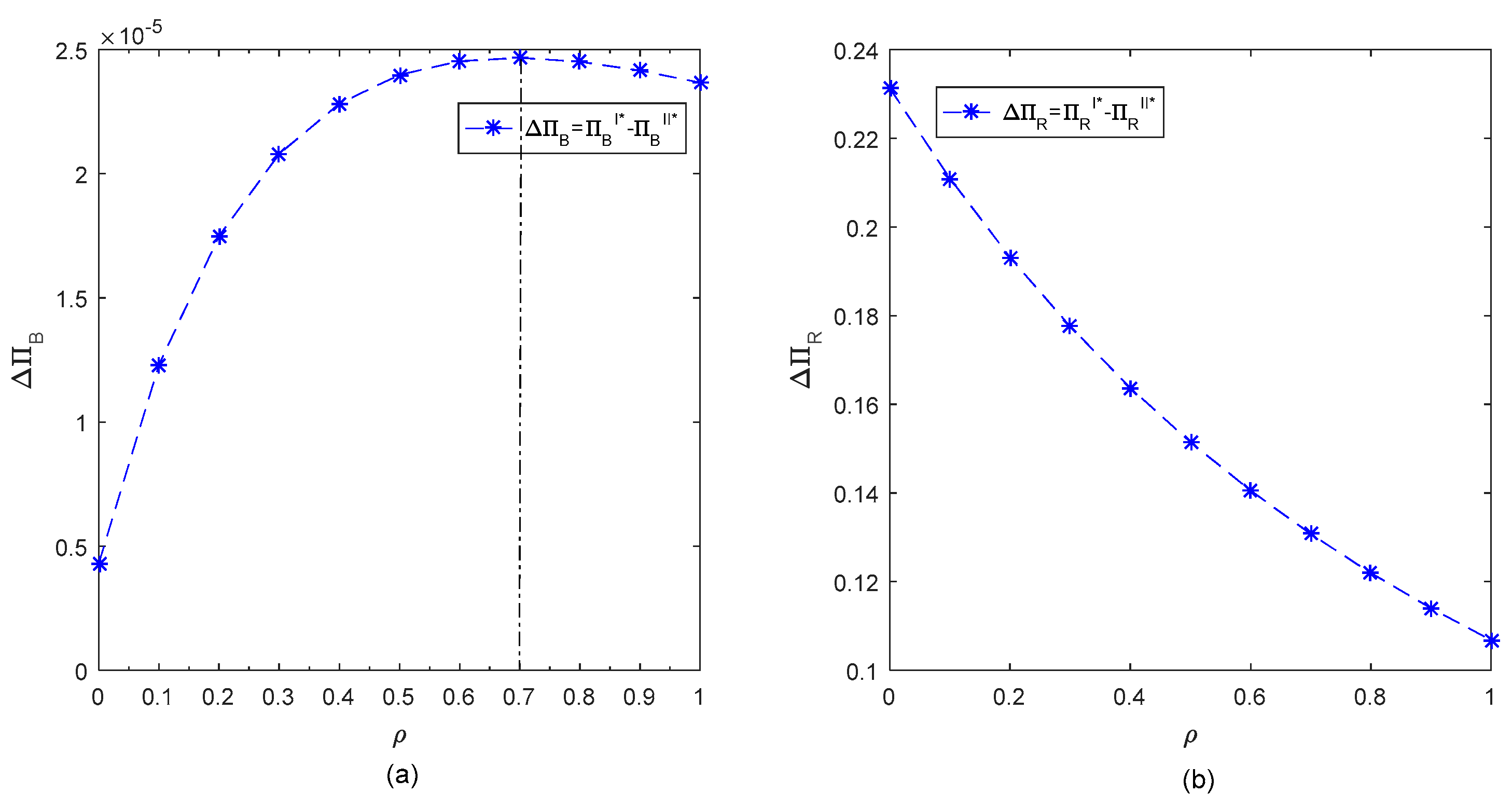
Due to the complex profit expressions of the bank and retailers, we comparex the profits of the bank and retailers in Case I with those in Case II through a numerical study. To obtain clear comparison results, we defined

$$\mathsf{\Delta }{\Pi }_B={\Pi }_B^{I*}-{\Pi }_B^{II*}$$

(28)

$$\mathsf{\Delta }{\Pi }_R={\Pi }_{R_1}^{I*}\left(={\Pi }_{R_2}^{I*}\right)-{\Pi }_{R_1}^{II*}\left(={\Pi }_{R_2}^{II*}\right)$$

(29)

Next, we examined through numerical analysis how subsidy rate ($\tau$), supply correlation ($\rho$), and the degree of supply uncertainty affect $\mathsf{\Delta }{\Pi }_B$ and $\mathsf{\Delta }{\Pi }_R$, respectively.

We set the market size ($a$), the Consumer’s green preference ($\mathsf{\lambda }$), and the investment cost coefficient of green technology ($k$) at a moderate level (i.e., $a=10$, $\mathsf{\lambda }=0.5$, and $k=10$). The expected supply yield variability factor was 1 (i.e., $\mu =1$). Note that Table 2 gives the range of the parameters.

Figure 1, Figure 2 and Figure 3 show how subsidy rate ($\tau$), supply correlation ($\rho$), and supply uncertainty (${\delta }_y$) affect $\mathsf{\Delta }{\Pi }_B$ and $\mathsf{\Delta }{\Pi }_R$, respectively.

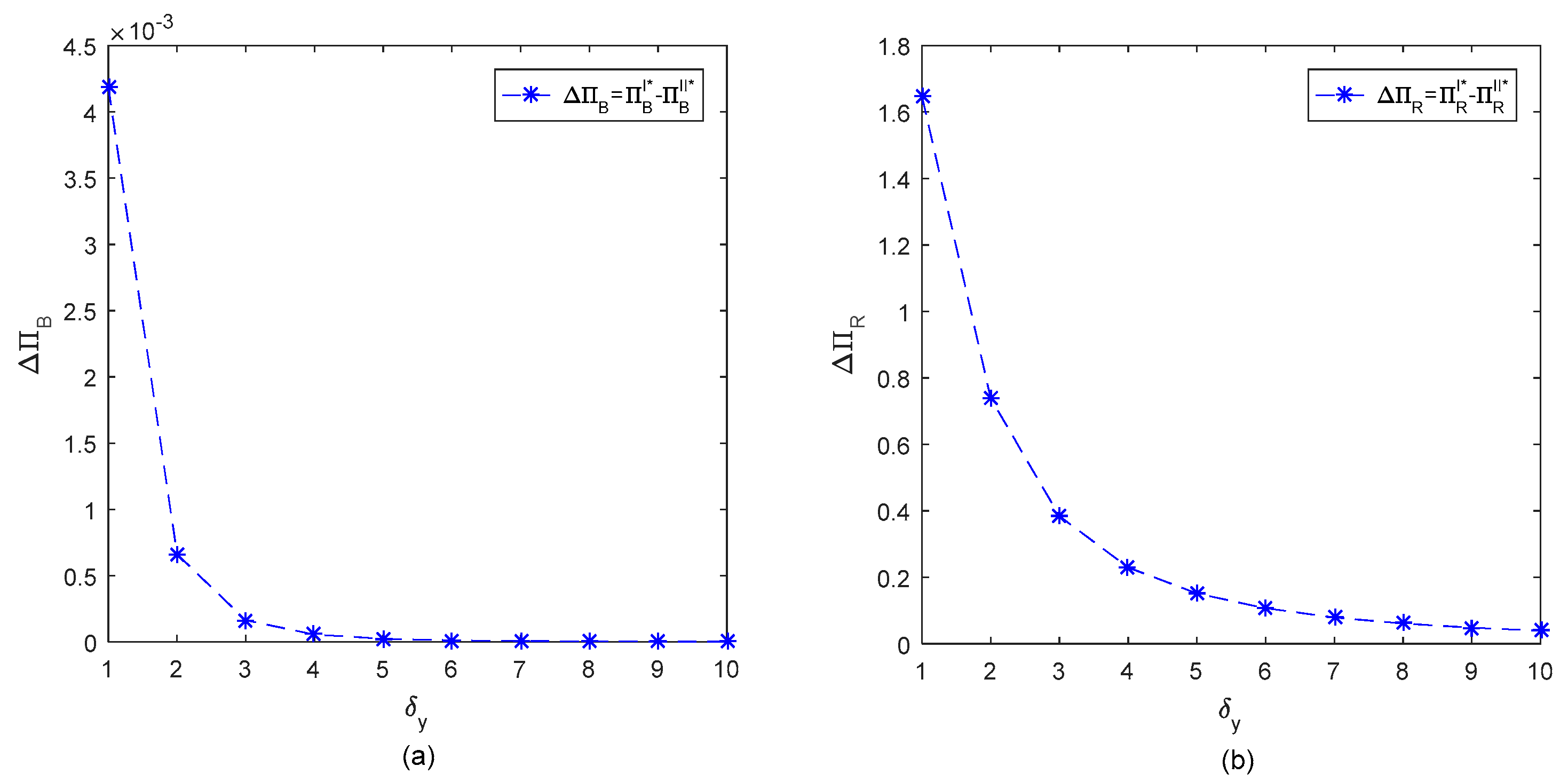
Figure 1, Figure 2 and Figure 3 show that both $\mathsf{\Delta }{\Pi }_B$ and $\mathsf{\Delta }{\Pi }_R$ are always positive. This means that the bank and retailers gain more profits in Case I than in Case II. This suggests that retailers who decide their order quantities independently can gain more profit than those who decide on the order quantity jointly with the alliance. Figure 1 shows that, as $\tau$ increased, the change trend of $\mathsf{\Delta }{\Pi }_B$ was the opposite to that of $\mathsf{\Delta }{\Pi }_R$. Figure 2 shows that, when $\rho <0.7$, the impacts of $\rho$ on $\mathsf{\Delta }{\Pi }_B$ and $\mathsf{\Delta }{\Pi }_R$ were the opposite. Otherwise, the impact was positively correlated. Figure 3 shows that the impacts of ${\delta }_y$ on $\mathsf{\Delta }{\Pi }_B$ and $\mathsf{\Delta }{\Pi }_R$ were in the same direction. This suggests that, when $\tau$ (lower $\rho$ and lower ${\delta }_y$) is low, retailers prefer competition to cooperation.

5.3. Social Welfare and Consumer Surplus

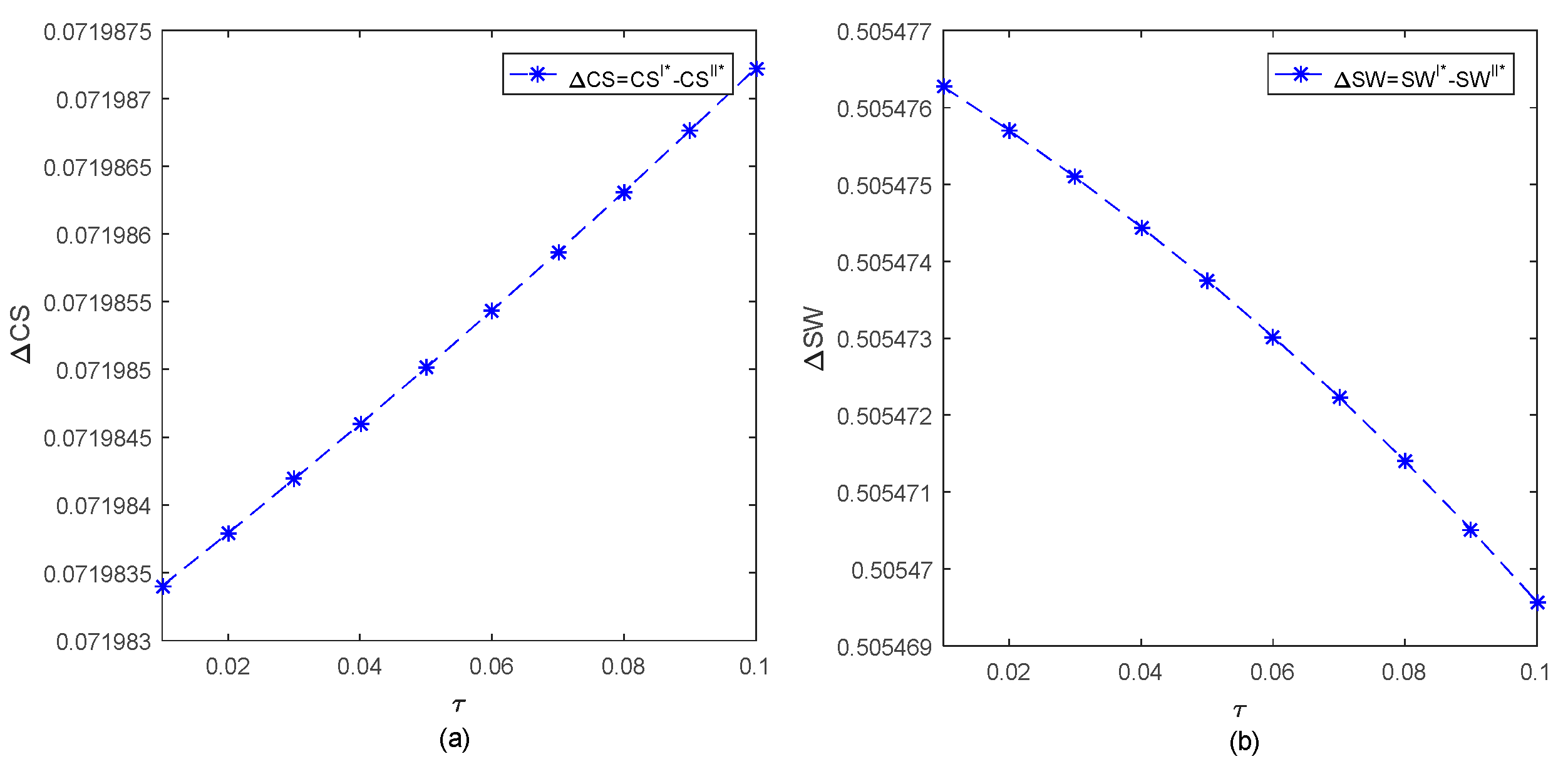
In this subsection, we compare the consumer surplus and social welfare between Case I and Case II. To obtain clear comparison results, we defined

$$\mathsf{\Delta }CS=C{S}^{I*}-C{S}^{II*}$$

(30)

$$\mathsf{\Delta }SW=S{W}^{I*}-S{W}^{II*}$$

(31)

Figure 4, Figure 5 and Figure 6 show how $\tau$, $\rho$, and ${\delta }_y$ affect $\mathsf{\Delta }CS$ and $\mathsf{\Delta }SW$.

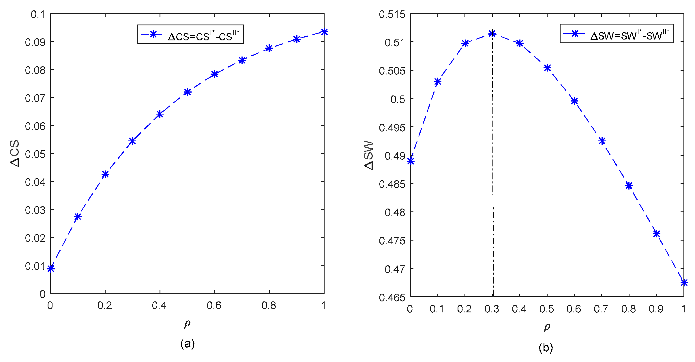
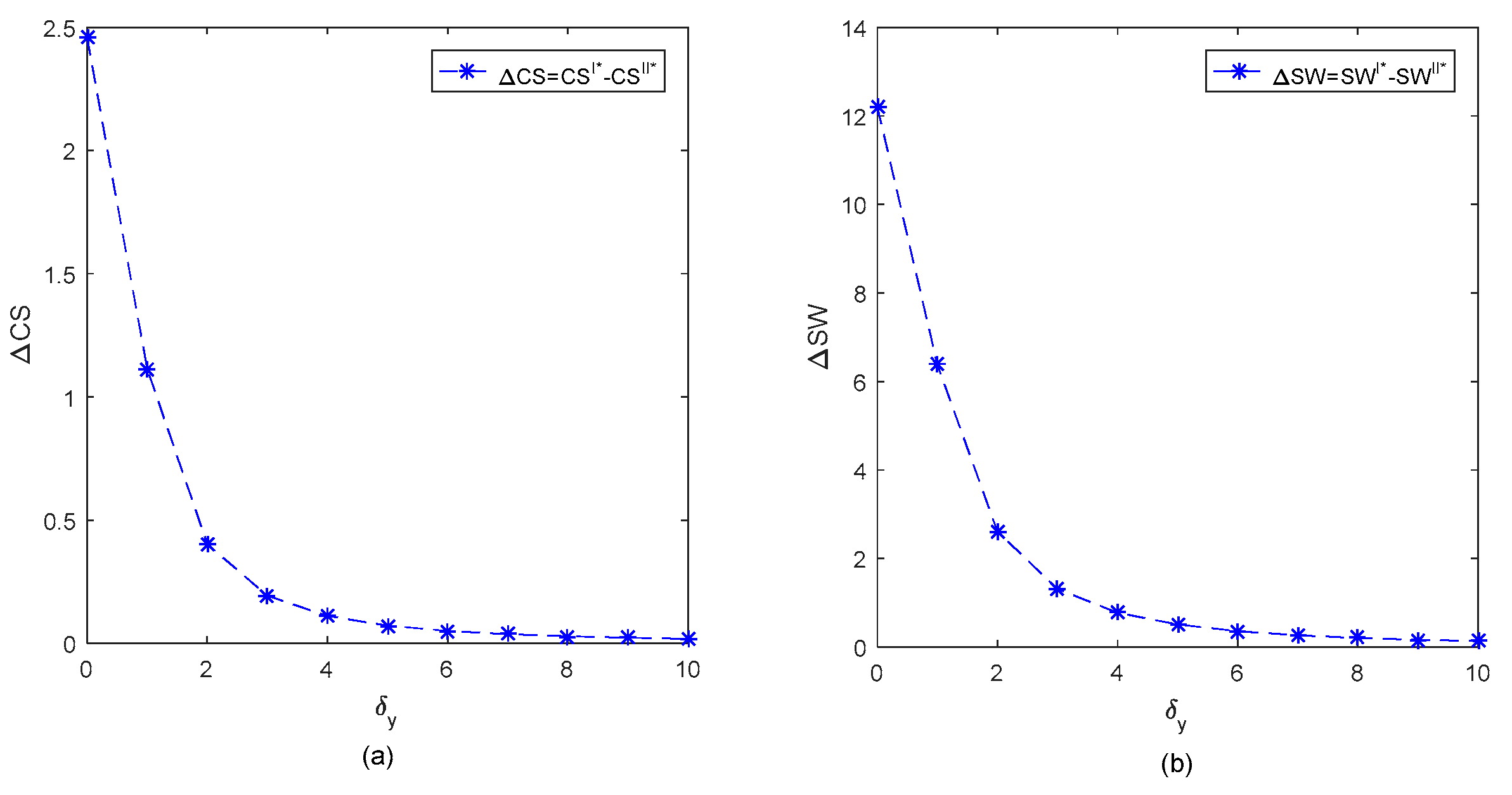
Figure 4, Figure 5 and Figure 6 show that both $\mathsf{\Delta }CS$ and $\mathsf{\Delta }SW$ are always positive, indicating that consumer surplus and social welfare in Case I are higher than those in Case II. Figure 4 shows that, under some condition (e.g., $\rho =0.5$ and ${\delta }_y=5$), $\tau$ affected $\mathsf{\Delta }CS$ and $\mathsf{\Delta }SW$ in the opposite direction. Figure 5 shows that, when $\rho >0.3$ ($\rho <0.3$), $\rho$ affected $\mathsf{\Delta }CS$ and $\mathsf{\Delta }SW$ in the opposite (same) direction. Figure 6 shows that ${\delta }_y$ affected $\mathsf{\Delta }CS$ and $\mathsf{\Delta }SW$ in the same direction. This suggests that, when retailers decide their order quantities independently (i.e., horizontal competition, case I), they can gain more profit than when they decide the order quantity via a planner of their alliance (i.e., horizontal cooperation, case II). When $\tau$ (moderate $\rho$ and lower ${\delta }_y$), retailers prefer competition rather than cooperation when social welfare is a performance metric.

6. Conclusions and Contributions

This study investigates green credit financing (GCF) in a green supply chain (GSC) with government subsidy and supply uncertainty. The GSC system is composed of one bank, one manufacturer, two retailers, and the government. The manufacturer uses GCF to mitigate the shortage of capital. The two retailers decide their order quantities independently (i.e., horizontal competition, case I) or via a planner of their alliance (i.e., horizontal cooperation, case II). The government provides subsidies to banks for using GCF.

We contributed to GCF study in GSC management. Our findings can guide manufacturers in making green product investment decisions. The bank decides the interest rate and the retailers decide order quantities accordingly (see Propositions 1 and 3). Our findings also suggest that, when the government’s subsidy rate is high (or the supply uncertainty is low or the supply correlation is low), the bank can set a low interest rate. With a lower financing cost, the manufacturer can set a higher product green degree. High product green degree corresponds to high investment cost in green productsa. Thus, the manufacturer sets a high wholesale price. Higher product green degree leads to higher demand; thus, the two retailers will set higher quantities (Corollaries 1–6).

The second contribution is related to retailers’ order mode choices: ordering independently (Case I) or jointly making a decision with the other retailer (case II). We found that the bank and SC members are better off in profits under Case I (retailers adopting horizontal competition) than under Case II (forming a partnership). This also suggests that under Case I, the manufacturer will invest more in green products and set a higher wholesale price; the bank will set a lower interest rate; and the retailers will order a higher quantity (see Propositions 5–6). Our findings also reveal that when retailers decide their order quantities independently (Case I), they can gain more profit than when they make order quantity decisions jointly (case II) (see Figure 1, Figure 2 and Figure 3). The corresponding consumer surplus and social welfare rates are both higher in Case I than in Case II. When subsidy rate is low, retailers would prefer competition to cooperation from a social welfare perspective (see Figure 4). The same observations can be made when supply correlation is moderate and supply uncertainty is low. See Figure 5 and Figure 6, respectively.

The final contribution of our work is in helping the government make subsidy decisions. The government’s subsidy strategy can effectively encourage manufacturers to invest in green products. This proves that the subsidy strategy is an effective tool to incentivize investment in green products. A high subsidy rate encourages the manufacture to invest more in green products. All findings in this research could provide valuable insights for the management of capital constrained GSCs with government subsidies and supply uncertainty.

Several limitations exist in this research. First, we considered the upstream manufacturer with limited capital. An interesting future research direction is considering the cases when the downstream SC retailers are also subject to limited capital and when the downstream businesses engage in Bertrand competition. Second, we assumed that the market demand is certain. In the future, we can further consider the downstream retailer’s own private demand forecast information and examine how the upstream capital-constrained enterprise’s financing strategy could affect the downstream retailers’ information sharing strategy. Third, we could study the manufacture’s financing decisions when government subsidy rate is endogenous and we could investigate the financing decision in a low-carbon supply chain under carbon tax and carbon trading policies. Finally, we could further explore the interaction among multi-sourcing, information sharing, and financing in a setting, with multiple capital-constrained unreliable suppliers and multiple retailers who own private demand forecast information.

References

- An, S.; Li, B.; Song, D.; Chen, X. Green credit financing versus trade credit financing in a supply chain with carbon emission limits. Eur. J. Oper. Res. 2021, 292, 125–142. [Google Scholar] [CrossRef]
- Huang, S.; Fan, Z.-P.; Wang, X. Optimal financing and operational decisions of capital-constrained manufacturer under green credit and subsidy. J. Ind. Manag. Optim. 2021, 17, 261–277. [Google Scholar] [CrossRef] [Green Version]
- Ling, S.; Han, G.; An, D.; Hunter, W.C.; Li, H. The Impact of Green Credit Policy on Technological Innovation of Firms in Pollution-Intensive Industries: Evidence from China. Sustainability 2020, 12, 4493. [Google Scholar] [CrossRef]
- Deng, L.; Yang, L.; Li, W. Impact of Green Credit Financing and Carbon Emission Limits on the Supply Chain Based on POF. Sustainability 2021, 13, 5814. [Google Scholar] [CrossRef]
- Jung, S.H. Offshore versus Onshore Sourcing: Quick Response, Random Yield, and Competition. Prod. Oper. Manag. 2019, 29, 750–766. [Google Scholar] [CrossRef]
- Tang, R.; Yang, L. Impacts of financing mechanism and power structure on supply chains under cap-and-trade regulation. Transp. Res. Part E Logist. Transp. Rev. 2020, 139, 101957. [Google Scholar] [CrossRef]
- Shen, B.; Wang, X.; Cao, Y.; Li, Q. Financing decisions in supply chains with a capital-constrained manufacturer: Competition and risk. Int. Trans. Oper. Res. 2019, 27, 2422–2448. [Google Scholar] [CrossRef]
- Deng, S.; Gu, C.; Cai, G.; Li, Y. Financing Multiple Heterogeneous Suppliers in Assembly Systems: Buyer Finance vs. Bank Finance. Manuf. Serv. Oper. Manag. 2018, 20, 53–69. [Google Scholar] [CrossRef]
- Lu, X.; Wu, Z. How taxes impact bank and trade financing for Multinational Firms. Eur. J. Oper. Res. 2020, 286, 218–232. [Google Scholar] [CrossRef]
- Jing, B.; Chen, X.; Cai, G.G. Equilibrium Financing in a Distribution Channel with Capital Constraint. Prod. Oper. Manag. 2012, 21, 1090–1101. [Google Scholar] [CrossRef]
- Cai, G.G.; Chen, X.; Xiao, Z. The Roles of Bank and Trade Credits: Theoretical Analysis and Empirical Evidence. Prod. Oper. Manag. 2014, 23, 583–598. [Google Scholar] [CrossRef]
- Chen, X. A model of trade credit in a capital-constrained distribution channel. Int. J. Prod. Econ. 2015, 159, 347–357. [Google Scholar] [CrossRef]
- Gao, G.-X.; Fan, Z.-P.; Fang, X.; Lim, Y.F. Optimal Stackelberg strategies for financing a supply chain through online peer-to-peer lending. Eur. J. Oper. Res. 2018, 267, 585–597. [Google Scholar] [CrossRef]
- Jin, W.; Zhang, Q.; Luo, J. Non-collaborative and collaborative financing in a bilateral supply chain with capital constraints. Omega 2019, 88, 210–222. [Google Scholar] [CrossRef]
- Kang, H.; Jung, S.-Y.; Lee, H. The impact of Green Credit Policy on manufacturers’ efforts to reduce suppliers’ pollution. J. Clean. Prod. 2020, 248, 119271. [Google Scholar] [CrossRef]
- Ding, W.; Wan, G. Financing and coordinating the supply chain with a capital-constrained supplier under yield uncertainty. Int. J. Prod. Econ. 2020, 230, 107813. [Google Scholar] [CrossRef]
- Zou, T.; Zou, Q.; Hu, L. Joint decision of financing and ordering in an emission-dependent supply chain with yield uncertainty. Comput. Ind. Eng. 2021, 152, 106994. [Google Scholar] [CrossRef]
- Yuan, X.; Bi, G.; Fei, Y.; Liu, L. Supply chain with random yield and financing. Omega 2021, 102, 102334. [Google Scholar] [CrossRef]
- Fang, L.; Xu, S. Financing equilibrium in a green supply chain with capital constraint. Comput. Ind. Eng. 2020, 143, 106390. [Google Scholar] [CrossRef]
- Huang, Z.; Liao, G.; Li, Z. Loaning scale and government subsidy for promoting green innovation. Technol. Forecast. Soc. Chang. 2019, 144, 148–156. [Google Scholar] [CrossRef]
- Li, Z.; Pan, Y.; Yang, W.; Ma, J.; Zhou, M. Effects of government subsidies on green technology investment and green marketing coordination of supply chain under the cap-and-trade mechanism. Energy Econ. 2021, 101, 105426. [Google Scholar] [CrossRef]
- Bian, J.; Zhao, X. Tax or subsidy? An analysis of environmental policies in supply chains with retail competition. Eur. J. Oper. Res. 2020, 283, 901–914. [Google Scholar]
- Yang, R.; Tang, W.; Zhang, J. Technology improvement strategy for green products under competition: The role of government subsidy. Eur. J. Oper. Res. 2021, 289, 553–568. [Google Scholar] [CrossRef]
- Bai, Y.; Song, S.; Jiao, J.; Yang, R. The impacts of government R&D subsidies on green innovation: Evidence from Chinese energy-intensive firms. J. Clean. Prod. 2019, 233, 819–829. [Google Scholar]
- Sun, H.; Wan, Y.; Zhang, L.; Zhou, Z. Evolutionary game of the green investment in a two-echelon supply chain under a government subsidy mechanism. J. Clean. Prod. 2019, 235, 1315–1326. [Google Scholar] [CrossRef]
- Zhang, J.; Wang, Z.; Zhao, H. The Impact of Consumer Subsidy on Green Technology Innovations for Vehicles and Environmental Impact. Int. J. Environ. Res. Public Health 2020, 17, 7518. [Google Scholar] [CrossRef]
- Li, Y.; Tong, Y.; Ye, F.; Song, J. The choice of the government green subsidy scheme: Innovation subsidy vs. product subsidy. Int. J. Prod. Res. 2020, 58, 4932–4946. [Google Scholar] [CrossRef]
- Dong, C.; Liu, Q.; Shen, B. To be or not to be green? Strategic investment for green product development in a supply chain. Transp. Res. Part E Logist. Transp. Rev. 2019, 131, 193–227. [Google Scholar] [CrossRef]
- Jung, S.H.; Feng, T. Government subsidies for green technology development under uncertainty. Eur. J. Oper. Res. 2020, 286, 726–739. [Google Scholar] [CrossRef]
- Guo, S.; Choi, T.-M.; Shen, B. Green product development under competition: A study of the fashion apparel industry. Eur. J. Oper. Res. 2020, 280, 523–538. [Google Scholar] [CrossRef]
- Ren, D.; Guo, R.; Lan, Y.; Shang, C. Shareholding strategies for selling green products on online platforms in a two-echelon supply chain. Transp. Res. Part E Logist. Transp. Rev. 2021, 149, 102261. [Google Scholar] [CrossRef]
Figure 1.
(a) The impact of on with and ; (b) the impact of on with and .
Figure 2.
Figure 3.
Figure 4.
Figure 5.
Figure 6.