
Urban Containment Planning: Is It Effective? The Case of Portland, OR

Department of Architecture, University of Florence, 50100 Florence, Italy
Sustainability 2021, 13(22), 12925; https://0-doi-org.brum.beds.ac.uk/10.3390/su132212925
Submission received: 27 August 2021
/
Revised: 5 November 2021
/
Accepted: 8 November 2021
/
Published: 22 November 2021
(This article belongs to the Section Sustainable Urban and Rural Development)
Abstract
:The paper attempts to evaluate Oregon’s and Portland’s growth management policies as for their tradeoffs between effectiveness in containing urban sprawl and impacts on housing markets and on property values. Carruthers argued that in order to correctly evaluate growth management policies, it is necessary to jointly consider their effects on urban development patterns, on land and housing markets, and on the fragmentation of land use controls. Nowadays, we have sufficient empirical research to evaluate the effects of Oregon’s growth management policies both on land markets and housing affordability and on urban development patterns. Therefore, the time has come to comprehensively reanalyze this longstanding case of public regulation. Once again, the issue of comparing grounded-on-planning–regulations’ effectiveness with grounded-on-price regulations’ effectiveness is at stake. The paper finds that urban-containment centralized-planning in Portland and Oregon have not been effective in containing sprawl and that price-based mechanisms are the most logical solution to the excess of sprawling urban growth.
Keywords:
urban containment; urban growth boundaries; sprawl; Portland; Oregon; housing markets; price signals1. Introduction
Urban containment is one of the mainland-use-planning goals. Contemporary urbanism arose from the social issues and from the urban problems determined by the industrial revolution, and its main product has probably been the idea of separating the various activities on land through zoning. In parallel to this and to other sanitarian issues arouse the need for compacting cities, as the natural tendency of settlements to sprawl tied itself to massive dimensional growth and was facilitated by the mass diffusion of cars.
In Great Britain, the entire planning system of the twentieth century was directed towards urban containment through the dual system of greenbelts and new towns. Later on, it was followed by various regions in countries as diverse as South Korea and the United States, Canada, Australia, Argentina, and Germany. Other planning schemes, such as the grid and the linear city, have been conceived and applied in various places to provide order, shape, and compactness to urban growth.
In the last fifty years, the urban containment frontier moved from Europe and Great Britain to the US, since Europe was demographically stagnant, while the US has a strong population growth. Today, the contemporary urban planning debate in the US is largely devoted to sprawl causes and costs and to policies to curb and contain it [1]. More recent research also investigates the relationship between settlement form and climate change [2,3,4,5]. The growing number of studies on the topic, however, does not allow for a clear correlation between sprawl and increased GHG production [6].
Within this more general debate, the Oregon case has an outstanding position. In fact, urban containment policies have been implemented in Oregon for over thirty years. Although the effects of Oregon’s urban containment policies on real estate markets and on urban sprawl were studied by many scholars, there was no comprehensive evaluation, which simultaneously considers the interdependencies between these two urban policies. This is an important gap, since the Oregon planning system is considered by many as an effective model to be diffused and imitated.
In this paper, I will try to fill this gap, analyzing the simultaneous effects of urban containment on real estate markets and urban sprawl. The next section summarizes the debate on sprawl and on urban containment in the US and describes Oregon’s legislation and Portland’s urban containment policies. The third section is devoted to analyzing the effects of such policies on land and housing markets and on urban dispersion. The fourth section discusses the shortcomings of such policies. The conclusive section draws policy implications and proposes an approach to urban sprawl based on price signals.
2. Materials and Methods
The paper uses case study research to investigate the effectiveness and potential problems of urban containment policies in the US political-administrative context. The case study chosen to conduct this evaluation was that of urban containment policies in Oregon and the Portland metropolitan area. The choice of the case study was based on the considerable amount of quantitative and qualitative research that has made it possible, over time, to evaluate the effects of these policies from different perspectives. In fact, urban containment policies were implemented in the Oregon and Portland metropolitan area in the 1970s, making this an almost unique case of urban development regulation in the United States and even in Europe. In particular, this study conducts an analysis of the cross effects of urban containment policies on the housing market and housing costs on the one hand and on the urban form on the other. This analysis is complemented by a review of comparative analyses of urban development and the housing market in the Portland metropolitan area and other metropolitan areas in the United States. Although this study relates to a specific context, its policy implications can be easily applied to similar cases of urban containment policies that are implemented nowadays in the US and in several other countries.
2.1. Sprawl Debate and Urban Containment Policies in the US
The term urban sprawl is used by politicians and the media all over the world, often imprecisely [7,8]. This phrase has a negative meaning due to the correlation—at times proven, at times only supposed—between urban sprawl and certain characteristics of dispersed settlements. Sprawl can be associated with several settlement configurations.
The reduction of density with distance from urban cores is theorized by land rent theory [9,10] and is embodied, in some ways, in all settlements. Therefore sprawl, in its negative meaning, is a matter of degree and not a problem per se [11].
The definition of conditions asserting that we are in the presence of negative sprawl is strictly tied to that of assessing its effects. This is a very complex task, and research provides no unquestionable answer. However, such assessment legitimates urban containment policies.
The term ‘sprawl’ is associated in the literature with 4 main settlement configurations: low-density development, ribbon development, scattered development, and leapfrog development [12]. Since sprawl is a matter of degree, it can be difficult to distinguish between scattered development and low-density development [13] (p. 662). Furthermore, the threshold, which identifies negative sprawl, can vary according to the city size. For example, over a certain size, scattered development may be more desirable than compact development, being seemingly connected to lower congestion [14,15].
In this paper, we are not going to cope with the issue of determining the thresholds, which allow us to consider sprawling settlements as negative. Therefore, we are going to assume the full legitimacy of urban containment policies.
Sprawl causes. Leapfrog development consists of developments, which bypass some land, leaving it undeveloped. This can occur, among other reasons, due to physical asperities, which make it difficult or expensive to develop, to regulations, which ban new construction, or to a landowner’s unwillingness to build.
It is interesting to consider sprawl causes in order to later evaluate the appropriateness of the remedies proposed to curb it. One of the main causes of sprawl is the independence of decisions made by developers who act atomistically in a competitive market. Each developer makes separate decisions according to remuneration expectations. Economic growth in a region causes developers to promote separate uncoordinated developments. Under such conditions, the higher the growth rate and the number of developers, the higher the expected number of casually set up developments [16].
Leapfrog development can be a byproduct of speculative wait by landowners who withdraw their parcels from the market, hoping to receive a higher remuneration in the future. If a city is experiencing significant growth, leapfrog development can be efficient in the long term when undeveloped areas are back on the market. In fact, the dimensional change of cities can require the redevelopment of inner areas, and this is more difficult if there are no voids to be filled in [17]. Research by Zhang et al. [18] on the Baltimore area over the period 1960–2005 empirically found this phenomenon, whose effects, however, were significantly diminished by zoning policies implemented after the late 1970s.
After having studied the speculative waiting phenomenon in Lexington land markets, Archer [19] concluded that the extra-profits for landowners were much higher than the social costs caused by such behavior. According to Archer, this behavior was partly due to the price policy applied by public service providers, to the incapacity of home buyers to foresee the transportation costs associated with their homes’ locations, and to the lack of revision of property taxes according to the actual value of the land. Such analysis introduces the theme of market distortions, which encourage sprawl.
Sprawl may also derive from a land conformation, which does not allow continuous urban development. In fact, urban growth tends to be realized on land, which is easier and cheaper to develop. This proved to be a major cause of sprawl [20].
Land use regulations can foster sprawl in various ways. Usually, such regulations are applied to areas that are smaller than the housing markets in which they are located. If in certain communities regulations are more stringent than in other communities, development tends to migrate from the ones with more stringent rules to the ones with less stringent rules.
Many local authorities pass zoning laws, which besides containing the quantity of development, also impose low densities and ban the construction of row-houses and multi-family houses, actually promoting sprawl [21,22,23,24]. This issue is connected to that of property taxation: in fact, low-density developments—generally occupied by the middle class and by the upper class—have a revenue/cost ratio, which is much better than that of high-density developments—generally occupied by the lower classes.
Public transportation systems encourage ribbon development—one of the kinds of sprawl—along the public transportation routes. The construction of a toll-free Interstate highway system made accessible large outer areas at a much lower price than it would be if its costs were to be paid through tolls by its actual users, subsidizing, in fact, urban sprawl. Besides being consistent with basic economic principles, this is confirmed, albeit indirectly, by Moynihan’s finding [25] that higher energy (and thus transportation) costs tend to reduce sprawl. A failure to anticipate future energy prices is likely to lead to sub-optimal choices that diminish future social welfare. Public policies, therefore, should anticipate wherever possible the impact of prices on sprawl ex ante, in order to maximize economic efficiency and minimize negative externalities from diffuse development.
Another subsidy, which affects sprawl is the deductibility from the income of mortgage costs and property taxes. If, on the one hand, that is desirable, on the other hand, it makes it affordable to buy larger lots, producing lower density [26] (p. 2). Furthermore, mortgage guarantee programs used to give preference to investments in newly-built single-family homes rather than in existing homes, row-houses, and multi-family houses [27].
Public services are usually priced based on the average cost rather than on the marginal cost. The more compact settlements close to the city center tend to cost less than the outer and more sprawled settlements. The effect of this is that compact city dwellers subsidize suburban residents, who are very often much more affluent.
Urban containment policies. In the first half of the twentieth century in the US there was widespread skepticism about regional planning and urban containment policies. Until the 1970s, the debate surrounding the effects of dispersed urbanization was mainly limited to the urbanization costs. In one of the earliest issues of the American Planners’ Journal, Raymond Unwin [28] (p. 46) dealt with this practical issue, counteracting with subtle irony to the supporters of multi-family houses: “Some critics who particularly dislike open building decry the density of twelve houses to the acre and quote the crescents of Bath as good examples of close building, oblivious of the fact that these have a density far less than twelve houses to the acre. There is, in fact, no relation of cause and effect between the adoption of the density of twelve houses to the acre and scattered building. The advocates of that density for small dwellings have consistently resisted scattered building, among other reasons because it is needlessly expensive in road and service costs, wasteful in effective garden space, and destructive of amenity. That density secures a spacing of the rows of dwellings, which gives the full benefit of sunlight and of freedom from intrusion on privacy and quiet from the houses opposite. While it benefits the landowner by bringing more land into use, it is, owing to road economies and a large increase in the area of available land as compared with higher densities, able to offer to the occupants value far in excess of the cost per plot of the extra land, which cost is easily covered by a fraction of the garden produce.”
Although Unwin’s opinion dates back to the 1930s, it is very representative of the attitude towards urban dispersion in the US, at least up to the 1960s. The preference for single-family homes was to be joint with urbanization costs control, without resorting to foreign solutions. After all, in the first half of the XIXth century, whereas in Europe the prevalent idea was to concentrate development and to preserve as much open space as possible [29,30], in the US, Frank L. Wright imagined dissolving the city in the country, in what we might call today a gigantic sprawl.
In the course of the 1960s, new chapters in state planning began, in which there was room for urban containment policies. This period is known in the literature as the “quiet revolution”, from the title of a book by Bosselman and Callies [31]. In 1961, Hawaii became the first state to enact a planning law, which required classification of all land in the state into land use districts and set the goals of compact development and of open space preservation [32]. A more fundamental change occurred between the end of the 1960s and the end of the 1970s, when also Oregon (1969, 1973), Florida (1975), and Rhode Island (1978) enacted similar laws.
Around the half of the 1980s, a second phase in the US urban containment policies started [33]. It began with the revision of the Florida planning law in 1985 and proceeded with the enactment of new planning laws in New Jersey (1986), Maine (1988), Vermont (1988), Rhode Island (1988), and Georgia. In this second phase: “Add the elusive but still very real concept of “quality of life”; articulate its expression through demands that infrastructure, especially transportation, be adequate to support the impact of development; add a steadily growing demand for affordable housing efforts as part of the picture; and you have the key ingredients of the “second wave” of state actions in planning and growth management.” [34] (p. 32).
The last phase, still ongoing, of the debate about urban containment, is influenced by the Smart Growth movement, which is very popular in the US. The interest in the issue of urban containment, which is still going on, is associated nowadays with more general attention towards neighborhood livability and accessibility [35].
2.2. Oregon’s Urban Containment Policies
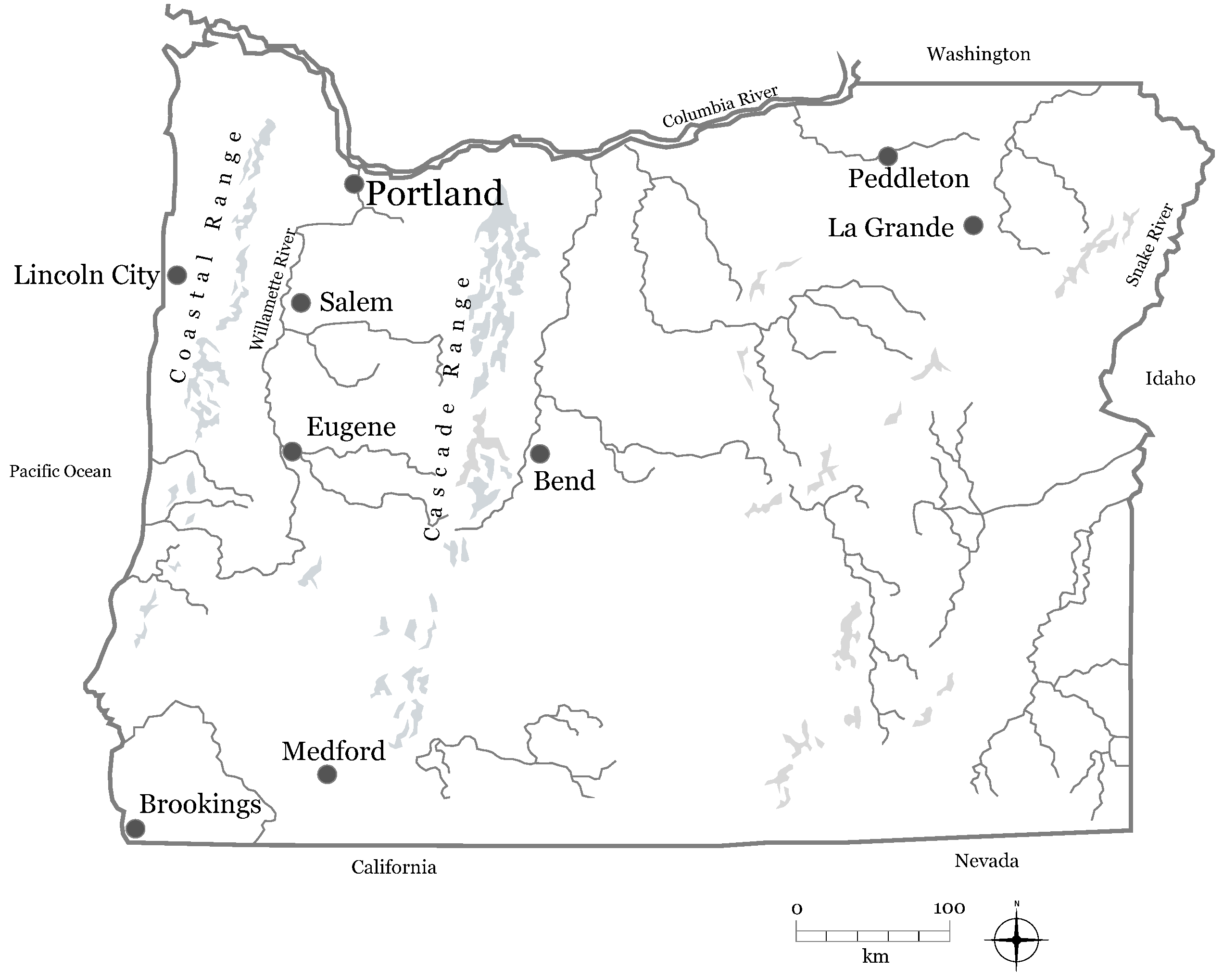
The State of Oregon is in the north-western region of the US. It is located on the Pacific coast with Washington to the north, California to the south, Nevada to the south-east, and Idaho to the east. Oregon’s capital is Salem, whereas the largest city is Portland, with an urban population of 662,549 (estimate 2021) and a metropolitan population of 2,151,000 (2020).
Oregon is very diverse and strongly reflects its geological makeup. Oregon is on the edge of the north-western continental plate, and its compression produced the Coastal Range and the Cascades Range. These two north-south ranges delimit the Willamette Valley, dividing it from the coastal region and from the scarcely inhabited rural area in the East (Figure 1).
From the beginning of the 1990s, Oregon and Portland gained in the local and in the national imaginary an almost mythical status of ‘Eden’ and have been the subject of many enthusiastic reports in the press and the media. This now stereotypical view of Oregon and Portland hides a great diversity in the society and in the policy tools, which are being implemented here. In the last 50 years, the Oregon economy progressively shifted from a resource-based economy to a knowledge economy. This change probably contributed to the political and geographic division, which exists today in Oregon’s politics [36,37,38,39].
The Oregon Planning System. In 1973 the Oregon legislature enacted Senate Bill 100, which established the state planning system that is still in force. The Oregon program is hierarchic, flexible, centralized, bargained, public and homogenous:
- Hierarchic because urban containment goals are set by the state and imposed to local governments;
- Flexible, for these goals, are translated into urban policies only at the local level and can produce several outputs;
- Centralized, since the state has the last word on local plans, through a review process;
- Bargained, because the review process involves bargaining between state authorities and local authorities;
- Public, for it consists of public land-use plans, which draw lines and establish zones, instead of general behavioral rules;
- Homogenous, because the general urban containment discipline is provided for the entire state.
The Land Conservation and Development Commission is vested with the authority of defining the planning goals and of reviewing local plans. The establishment of such goals came after a long consultative process [40] (pp. 13–4). The goals addressed several issues, from resource territory to recreation, from economics to housing policies. Six goals define the urban containment policy: Goal 14—Urbanization, Goal 9—Economy of the state, Goal 10—Housing, Goal 11—Public facilities and services, Goal 12—Transportation, and Goal 3—Agricultural Lands.
Goal 14, Urbanization, requires local governments to calculate the need of developable land determined by population growth and to establish urban growth boundaries in order to contain it. Goal 10, Housing, aims at providing “the housing needs of citizens of the state” through the development of housing types at all “price ranges and rent levels” and through the provision of “financial incentives and resources to stimulate rehabilitation”. Goal 9, Economy of the State, ties the establishment of urban growth boundaries to the consideration of occupational opportunities and to their economic effects appraisal. Goal 11, Public Facilities and Services, sets to “to plan and develop a timely, orderly and efficient arrangement of public facilities and services” through the coordination of land-use-planning agencies and of public-facilities providers and through fiscal incentives/disincentives, and impact fees. Goal 12, Transportation, counts “to provide and encourage a safe, convenient, and economic transportation system”, also through the coordination of infrastructure planning and of urban planning. New roads, furthermore, should not go through prime agricultural land. Goal 3, Agricultural Lands, asks to identify prime agricultural lands and to prevent them from being divided into lots smaller than the size, which is enough to meet the needs of profitable agriculture.
The Enforcement of Senate Bill 100. The goals used by the LCDC to review comprehensive plans and sector plans set general principles, which need to be translated into policy and into programs. That is no simple task, for goals easily conflict with each other and there are often different ideas about the proper balance between them. The negotiation process between state power and local governments is also susceptible to conflicts between state goals and local interests and needs. Furthermore, interest groups try to exert their influence in different directions. Therefore, a goal set as the aforementioned one produces outputs, which are difficult to be forecasted.
To no one’s surprise, the review process of local plans by the state took 11 years more than originally forecasted, being completed in 1986 instead of 1975. Urban growth boundaries were often at the center of such disagreements: cities pushed for large UGBs, whereas counties—where farmers were influential—and environmental groups wanted to curtail them as much as possible. The Department of Land Conservation and Development usually was on the side of counties and asked cities to reduce UGBs. Such disagreements were resolved through negotiations, e.g., relaxing development regulations in agricultural land [41].
A second area of disagreement was related to residential zones. Local governments often adopted low-density plans with strict limits to high-density developments. The home builder’s associations and the environmental associations wanted higher densities and looser implementation rules. The Department of Land Conservation and Development often asked local governments to amend their plans in order to allow higher densities [41,42].
A third controversial issue was related to agricultural lands. County government plans loosely preserved agricultural lands, whereas environmental groups struggled for strict preservation standards. In addition, in such cases, the DLCD often asked county governments to introduce stricter regulations concerning developments outside UGBs [43].
According to Knaap [44], the review process by LCDC strongly affected local-plans contents, determining smaller UGBs, stricter standards for agricultural lands, and looser implementation-regulations for urban areas. Through this process, an implicit agreement between development interest-groups and environmental interest groups would have been reached in order to ease development within UGBs, while limiting it as much as possible in rural areas (ibidem). In the review process, local governments were partially deprived of their decision-making power. In the implementation process, they may regain some of their influence through the interpretation and the amendment of regulations and plans [45]. Because of this, there can be substantial differences between the plan, which is adopted and the one that is actually realized.
Much evidence shows that in Oregon there was a strong difference between what was asserted in the state planning goals and what was being realized locally through land-use plans. For example, over 85 percent of residential developments and over 96 percent of building permits issued between 1981 and 1989 were on prime agricultural land [44,46]. Furthermore, within UGBs, densities were lower than planned, whereas outside UGBs, the opposite was true [44,47].
2.3. Urban Policies and Urban Containment in the Portland Area
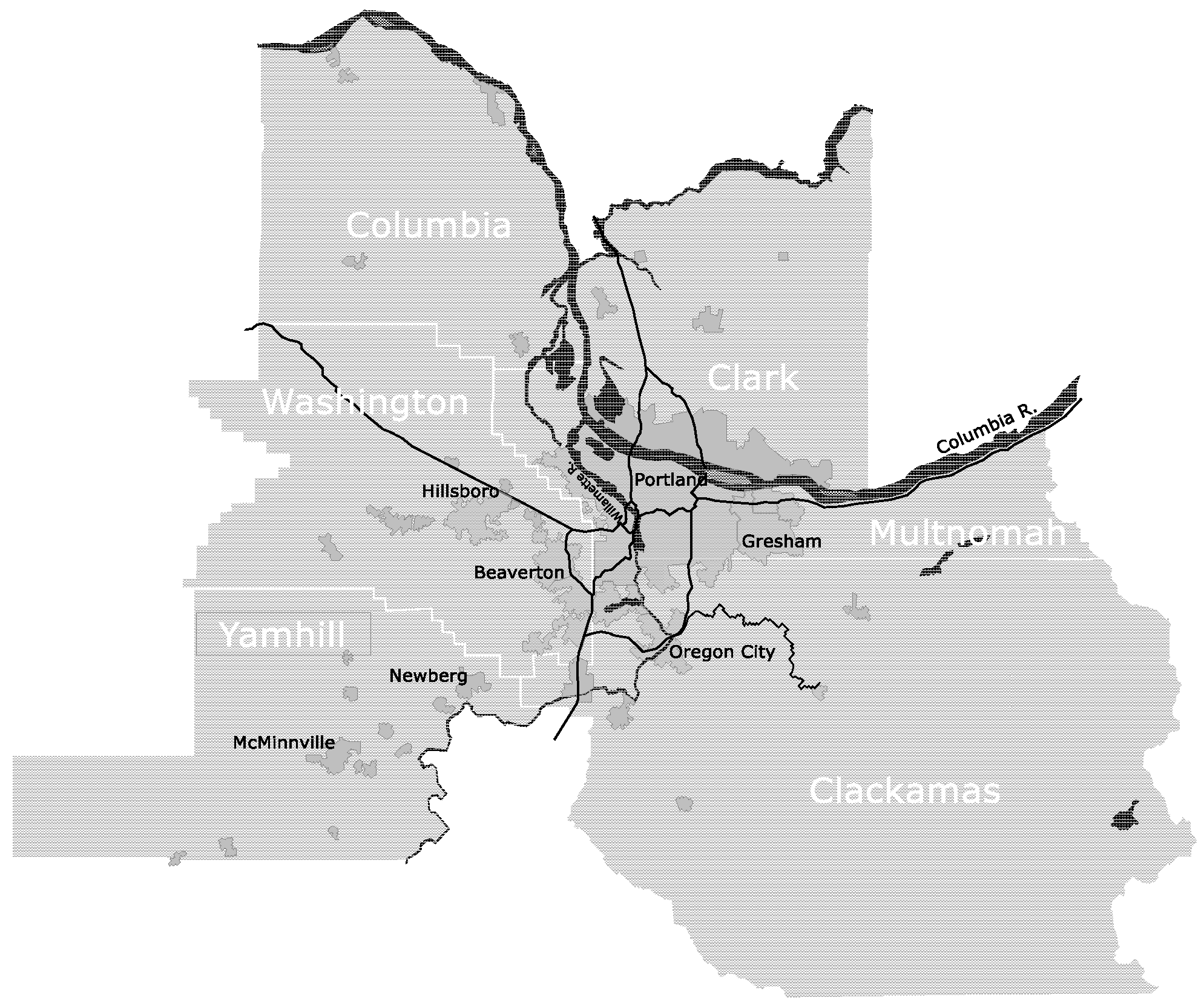
Portland is at the confluence of two big rivers, the Columbia River and the Willamette River, some 90 miles from the Pacific Ocean. It lies at the core of a metropolitan statistical area, which encompasses five Oregon Counties (Clackamas County, Columbia County, Multnomah County, Washington County, and Yamhill County) and Clark County in Washington State. In 2020 the population of the metropolitan area was 2,151,000.
Portland grew as an ocean harbor and as a regional service center. Up to the middle of the 19th century, the Willamette Valley was an overwhelmingly agricultural region, and the remainder of Oregon’s economy was mainly based on timber. During the two world wars Portland developed a flourishing naval industry. The harbor was used to export timber and agricultural products from this region and to import raw materials and finished products from the outside world. Everything in Portland revolved around the river. In the last 6 decades, Oregon’s economy became much more diverse, and the importance of river related-activities diminished over the years. Between 1980 and 1997 the percentage of jobs within one mile of the river decreased from 50% to 39%.
Urban containment in metropolitan Portland. In the mid-1970s, initiatives were undertaken in Oregon to study regional governance issues and options for metropolitan areas [48]. These initiatives led to the proposal of substituting the Council of Governments with an elected metropolitan government. In 1978 the proposal was approved by voters, and the following year, the first Metropolitan Service District Council, commonly known as Metro, was elected (Figure 2).
Metro is still the only elected regional government in the United States. Although in charge of various sectors, it has no power—in step with a tradition of local self-government, which is very rooted in the US—to draw up a comprehensive land-use plan. However, it can require local governments to amend their comprehensive plans to comply with its various sector plans.
In 1987, Metro initiated an evaluation of the UGB’s effectiveness. Such an evaluation was deemed necessary because it was clear that settlements were growing in a sprawling pattern, that many reserve areas were being developed, and that residential densities were lower than planned within UGBs and higher than planned outside UGBs.
The aforementioned research findings led to an extension of UGBs and to the creation of the Urban Growth Boundary Management Policy Advisory Committee, formed by representatives of Metro and of local governments, as well as from representatives of some interest groups. The Committee adopted some guidelines to be followed in the UGBs management, which were approved by Metro in 1991 [49,50].
In 1992, thanks to a constitutional amendment introduced in 1990, Metro adopted a home rule charter, which recognizes, among other things, its competency in administering the UGBs within its jurisdiction.
3. Effects of Oregon’s and Portland’s Urban Containment Policies
There are conflicting opinions among scholars about urban-containment effects on urban sprawl and on real estate markets [21,51,52]. Urban growth patterns are influenced by various policies, each with its goals, and political fragmentation is likely to reduce policy effectiveness. Urban containment policies have major effects on real estate markets and on urban growth patterns. Therefore they should be analyzed starting from their effects on land and housing prices and on urban development patterns.
Urban containment affects the amenities available to properties and impacts their prices and rents. Urban growth patterns can be studied, among other things, with reference to residential density and the total urbanized area.
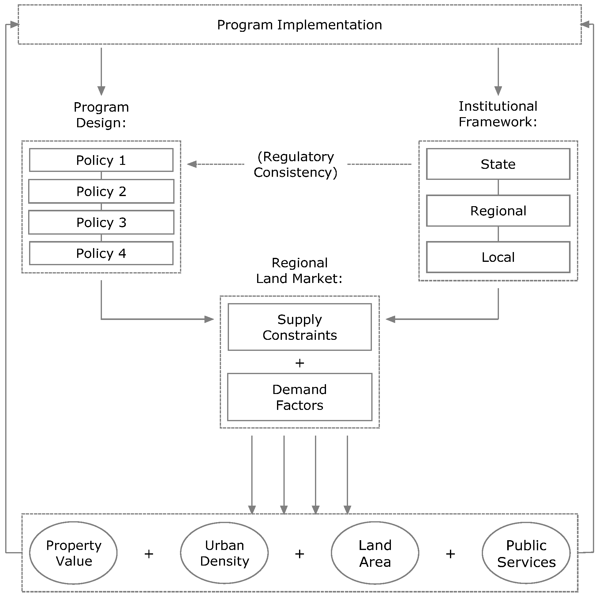
The scheme developed by Carruthers [1] synthesizes the major interdependencies among policies (growth management policies/land markets, institutional setting/land markets, land markets/urban growth patterns) and the major tradeoffs among policies (housing affordability and sprawl containment, infrastructure costs and land costs) and is of some utility in the evaluation of urban containment policies (Figure 3).
In this section, we discuss the effects of Oregon’s urban containment policies on real estate markets and on sprawl.
3.1. Effects on Land Markets
The effect of an urban growth boundary (UGB) on land markets is similar to the effect of a greenbelt on land markets. This effect has been described by Nelson [53]. In the presence of a greenbelt, land markets become segmented into two distinct markets: the market of developable land out of the greenbelt and the market of undevelopable land in the greenbelt.
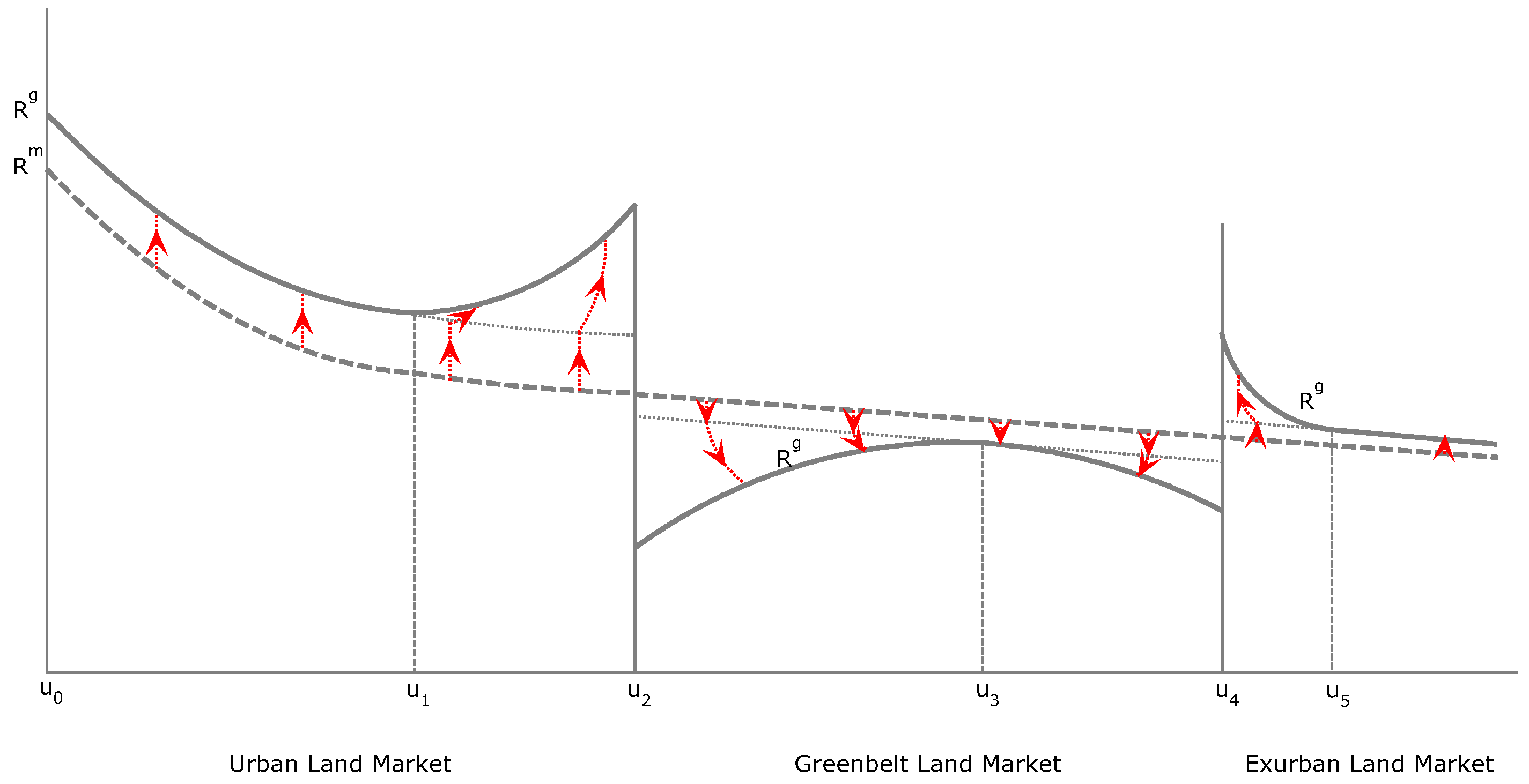
If the land is homogenous and there are no restrictions limiting development, the bid rent function, represented in Figure 4 by the curve Rm, decreases smoothly with increasing distance [9]. The establishment of a greenbelt divides the curve into three segments, pushing Rm upwards out of the greenbelt (between u0 and u2 and beyond u4) and pushing Rm downwards within the greenbelt (between u2 and u4). The upwards movement out of the greenbelt is due to the total reduction of the supply of developable land; the downwards movement within the greenbelt is due to the restriction, which prevents development. This effect is illustrated by the curve Rg.
Greenbelts increase the environmental quality of nearby neighborhoods [54], therefore increasing their land rent up to a certain distance from greenbelts (between u1 and u2, and between u5 and u4). Conversely, settlements around the greenbelt have a disturbance effect [55] on farmland productivity within the greenbelt, reducing their rent up to a certain distance from settlements (between u2 and u3 and between u4 and u3).
Therefore greenbelts (and UGBs) produce the effect of artificially redistributing wealth from the owners of land within greenbelts (outside UGBs) to the owners of land inside greenbelts (inside UGBs). Greenbelts and UGBs also reduce the supply of developable land, therefore, increasing its value. Being land one of the production factors of houses, housing prices can also increase. However, this effect is not automatic: in fact, various adjustments, both on the demand side and on the supply side, can be made.
Finally, greenbelts and UGBs do not grant any right to developing land, being this a prerogative of zoning codes. Therefore, after UGBs are established, it takes a longer time span for land to be developed. This produces three different land regimes: developable land inside UGBs; land inside UGBs, which is not yet developable; land outside UGBs.
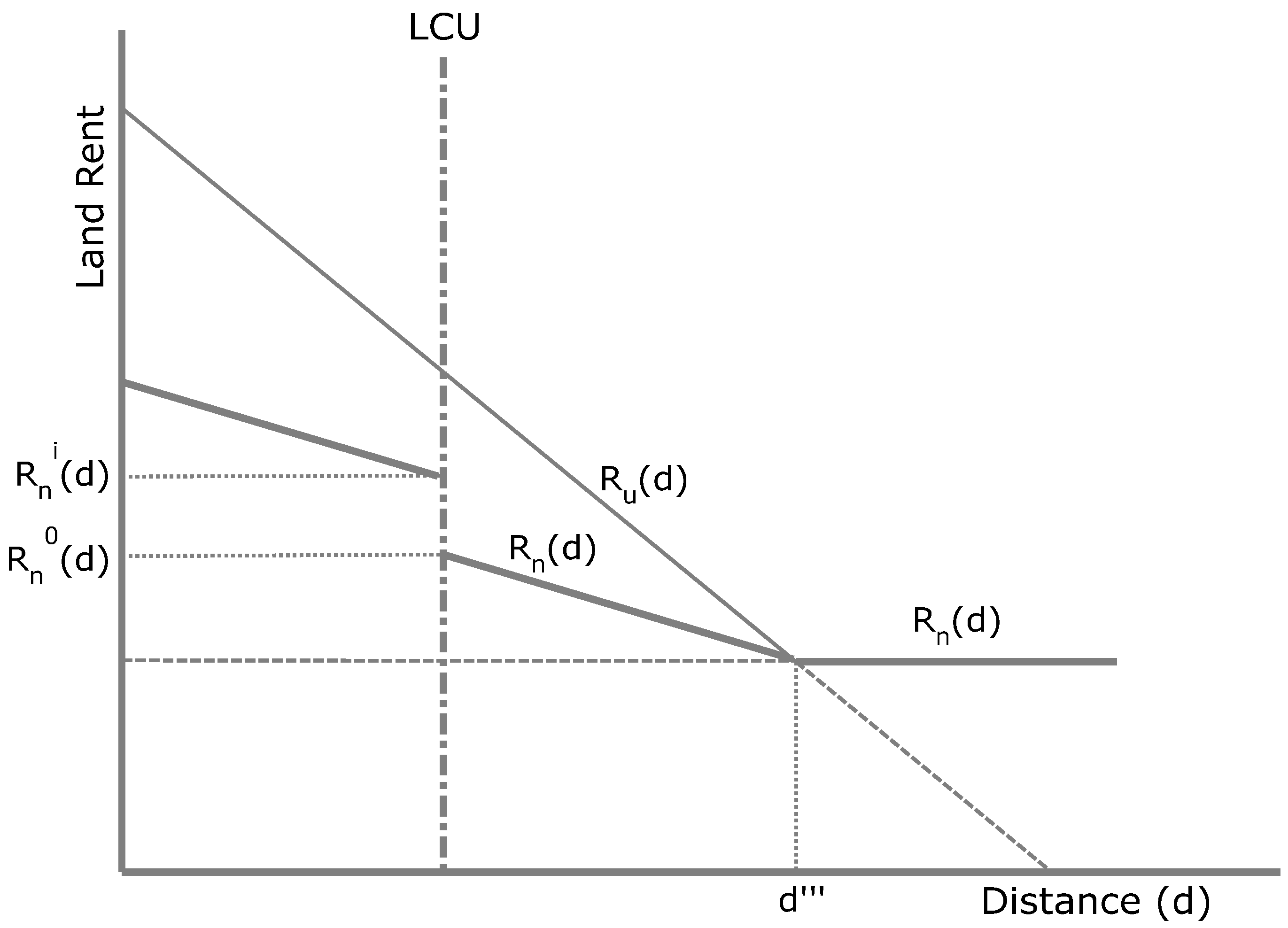
This segmentation effect of a UGB on land markets is represented in Figure 5. With some simplifying assumptions, without a UGB, the urban-land rent curve Ru decreases with distance d from the urban core, and the non-urban-land rent curve Rn is constant and independent from the place. The UGB has no effects on developable land value while having major effects on undevelopable land value. The bid-rent function is split into two segments: the segment inside the UGB is shifted upwards, whereas the segment outside the UGB is shifted downwards. The distance between the two segments equals the difference between the actualized value of the rent-stream Rni(d), which is supposed to be produced by land inside the UGB, and the rent-stream Rno(d), which is supposed to be produced by land outside the UGB. This difference depends on the time span between the right of developing land on the two sides of the UGB.
3.2. Effects on Housing Prices
With some degree of simplification, housing markets are comprised of property markets, asset markets, and housing building markets. These markets are strictly interdependent thus that changes in one of them are reflected by changes in the others.
Empirical research concerning the Salem land markets and the Portland land markets, although covering a limited time span, showed that UGBs can actually have an inflationary effect on developable land values. This effect manifests itself a certain time after the establishment of UGBs and can vary depending on local governments’ zoning.
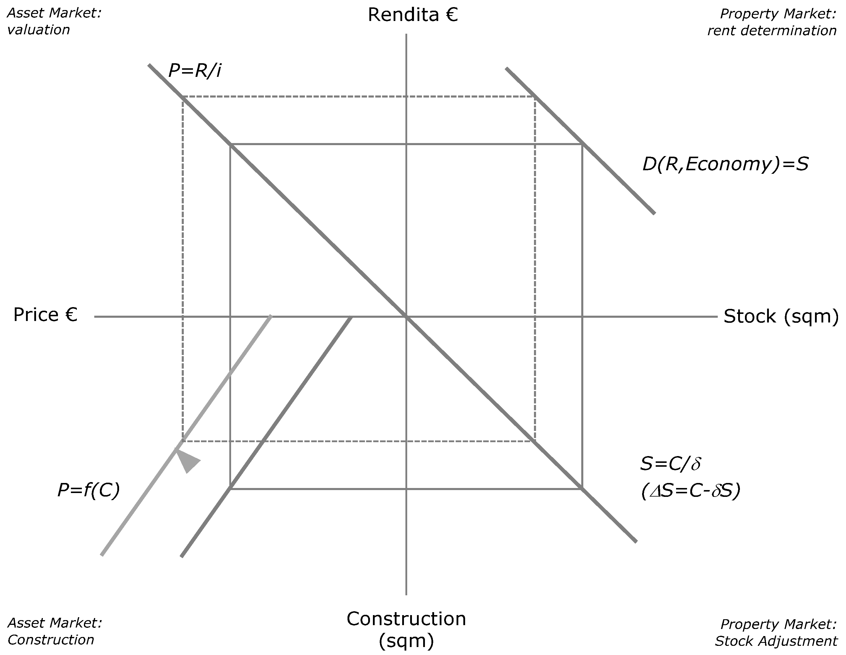
All else being equal, the increase of developable land prices determines an increase of the overall production costs and a clockwise rotation of the supply curve in the SW quadrant represented in Figure 6. With the same assumptions, this results in a housing-stock reduction and in an increase of housing rents and prices.
However, in the real world, it is highly probable that various adjustments occur, and it is necessary to determine all other UGBs effects. According to the economic theory, an increase in the cost of a production factor will induce producers to substitute this factor with other factors (substitution effect). If land values increase, developers tend to build on smaller lots. Therefore an increase in land values can result in an increase in density, a reduction of land per house, and in a qualitative change in the housing supply. Such a density increase can partially or wholly balance the land value increase. To make an example, if land, which cost 90 now costs 100, it is necessary to reduce lots size 10 percent to maintain equal their average cost incidence per housing unit.
In the 1990s, housing prices rapidly rose in Portland. In 1991 a housing unit cost, on average, $25,000 less than the US as a whole. In 1994 this gap was filled, and in 1996, a housing unit cost on average in Portland §25,000 more than in the US as a whole [58]. These data supported the idea that the housing price increase was due to the UGB, which was blamed for reducing affordable housing supply with serious social effects (Figure 6).
Although these data apparently left no doubt regarding the UGB’s effect on housing prices inflation in Portland, to really calculate this effect, it is necessary to correctly assign their causation to the many variables that may affect them. Three studies carried out in the last decade attempted to isolate UGB effects on Portland’s housing prices from the effects of other variables [58,60,61].
In the regression calculated by Phillips and Goodstein [60], the mean housing price in 1996 in 37 metropolitan areas across the US is a dependent variable of the population (sign +), median income (+), unemployment rate (−), climate mildness (+), construction cost (+), land availability (−), the number of municipalities (−), the pervasiveness of regulations (+), and the percentage change in prices in the period 1990–1995 (+). The pervasiveness of regulations is calculated using the Wharton regulatory index developed by Malpezzi [62]. The percentage change in prices in the period 1990–1995 was used to estimate the effect of speculation on housing prices. Two regressions were run with and without such variables.
The mean housing price in Portland estimated by the regression in 2000 was $124,424 without including the variable ΔP, and $147,933 including the variable ΔP. The actual mean housing price in Portland in 2000 was $144,000. The difference between the actual price and the estimated price in the equation without ΔP measures the cumulative effect of speculation and of UGB on housing prices. Of this difference, which is $19,576, Phillips and Goodstein assume that no more than $10,000 is directly due to the UGB.
In his work, A. Downs [58] used the housing price variation in five time intervals (1990–2000, 1990–1994, 1990–1996, 1994–2000, and 1996–2000) as a dependent variable in a sample of 86 metropolitan areas across the US. The goal was to assess how UGB’s impact on housing prices changes over time. A total of 25 independent variables were used in a first regression, selecting the ones with higher r2 values. A second regression calculates the percentage change of housing prices in each time period associated with each variable. Variables with low t-scores were also eliminated. Finally, a dummy variable ‘Portland’ was introduced, running the regression again.
In the case of the time intervals 1990–1994, 1990–1996, and 1990–2000, the dummy variable ‘Portland’ was statistically significant and was associated with high r2 scores. Instead, in the case of the time intervals 1994–2000 and 1996–2000, the introduction of the dummy variable produced no effects. The dummy variable ‘Portland’ might represent singularities associated with this city different than the UGB. To better assess this possibility, each city was used as a dummy variable in as many regressions. Since none of them was statistically significant, it is highly probable that the dummy variable Portland actually represents the UGB’s effect.
The result of the study, concludes A. Downs, was that the UBG had a significant impact on Portland housing prices only in the time interval 1990–1994, but not before 1990 and after 1994.
These results were not surprising since in the period 1990–1994, employment growth was strong both in Portland and in the US. Furthermore, the initially established UGB was very large, and its effect was to be perceived only over time. Finally, after 1994 population growth was slowing, and developers might have adapted to build on smaller lots.
The study carried out by Jun [61], unlike the previous studies, used disaggregated data for only the Portland area (instead of aggregated metropolitan data). The price in 1990 and in 2000 was assumed as a dependent variable, and UGB’s effect was controlled by using the UGB as a dummy variable. Since this dummy variable had no significant effect, the location of houses within or beyond the boundary did not influence their price. Therefore, even though the UGB segments land markets, it does not have the same effect on housing markets. Since this does not mean that UGB does not affect the mean housing price, this study adds nothing to Phillips and Goodstein [60] or to Downs [58].
3.3. Effects on the Urban Form
Oregon planning goals do not state the precise urban form which ought to be realized. Anyway, in the requirement “to provide for an orderly and efficient transition from rural to urban land use, [and] to accommodate urban population and urban employment inside urban growth boundaries” (Goal 14), we can recognize a criterion of urban-growth compactness and contiguity.
Public service policies also promote compact development patterns. State legislation requires that “lands within urban growth boundaries shall be available for urban development concurrent with the provision of key urban facilities and services in accordance with locally adopted development standards” (Oregon Revised Statutes § 197.752). Goal 11 requires local governments “to plan and develop a timely, orderly and efficient arrangement of public facilities and services to serve as a framework for urban and rural development”. The implicit idea is that public infrastructures and services can be efficiently provided only if new developments are realized in sequence on land which is contiguous to the existing settlements.
The promotion of urban compactness is more explicit if we consider the administrative rules for the UGB extension. These rules require, among other things, the establishment of urban reserve areas for future UGB expansion needs. In establishing urban reserve areas, the “first priority goes to land adjacent to, or nearby, an urban growth boundary and identified in an acknowledged comprehensive plan as an exception area or nonresource land” (Oregon Revised Statutes 660-021-0030).
To measure the effects of these policies on Oregon settlements’ compactness is very complex. In fact, it is necessary to define urban sprawl and to measure the way it changes over time due to these policies. The concept of sprawl embraces many dimensions, and sprawl definitions found in the literature are very diverse and, at times, also very complex.
Thus far, three studies define composite indexes aimed at measuring sprawl in its various dimensions [7,8,63]. Only the third, however, is applied to a sample of metropolitan areas, which includes the Portland-Vancouver Metropolitan Area and whose variation is calculated for the decade 1990–2000. It is not possible here to mention all the definitions of sprawl that occur in the literature. To provide an example, Galster and others [7] (p. 685) suggested the following definition: “Sprawl is a pattern of land use in UA that exhibits low levels of some combination of eight distinct dimensions: density, continuity, concentration, clustering, centrality, nuclearity, mixed uses, and proximity”.
Other studies measure sprawl using one variable or a very small number of variables. Some of these studies (e.g., [64]) compared a number of metropolitan areas and measured their sprawl variation over a certain time. Others looked for a correlation between urban containment policies adopted in a sample of US metropolitan areas and sprawl variation over a certain time [65,66,67,68]. A small group of studies compared only a few metropolitan areas, analyzing the correlation between urban dispersal and urban containment policies [69,70].
Paulsen [71] shifts the focus to what we might call the ‘marginal variation of sprawl’ by measuring four variables: urban housing unit density, marginal land consumption per new urban household, housing unit density in newly urbanized areas, and percent of new housing units located in previously developed areas. These are measured for 1980 and 2000 for all 329 metropolitan areas in the continental United States, which in turn have particularly diverse planning systems. To assess the correlation between planning policies and the marginal variation of sprawl, Paulsen uses the dummy variable ‘substantial state planning role’.
In their literature review on sprawl, Clifton et al. [72] pointed out that many studies on sprawl focus on neighborhoods. We may contend that this unit of analysis is too small to capture urban development trends. In any case, it enables us to understand how certain urban quality indicators—which were not considered in studies focused on the metropolitan level—change over time. For the Portland area, this kind of research was carried out by Song and Knaap [73].
3.4. Comparative Analyses with Other Metropolitan Areas
An insightful and provocative paper presented by Gordon and Richardson [70] in 2001 compared Portland and Los Angeles. In 2001, Los Angeles was still considered a metaphor for sprawl, and Portland was a metaphor for environmental-friendly urban growth. Gordon and Richardson [70] argued that the opposite holds true.
In 1990, residential density per square mile was 3.021 in Portland and 5.081 in Los Angeles, respectively. As shown by Fulton et al. [74], in the period 1982–1997, land consumption increased by 19.4 percent in Portland and by 6.5 percent in Los Angeles, whereas density decreased by 11.3 percent in Portland and increased by 2.8 percent in Los Angeles. As shown by Newman and Kenworthy [75], Portland has 2.8 times more road length per capita than Los Angeles. In the time period, 1992–1997 vehicle miles traveled increased by 25.2 percent in Portland and by 0.2 percent in Los Angeles. In the same five years, the travel time index, which measures the time-duration of trips, increased by 19 percent in Portland and by 1 percent in Los Angeles. In 1995, the average commuting time was 24.1 min in Los Angeles and 18.5 min in Portland, not a big deal if we consider the difference in the road length per capita and in the urban size.
After comparing the two metropolitan areas with respect to social diversity, immigration, and political fragmentation, Gordon and Richardson [70] concluded that Portland’s urban containment policies promote social homogeneity and serve the interests of the urban middle class but have no visible effects on urban-growth environmental impacts.
Pendall et al. [64] compared the sprawl variation, defined by a composite index, in a sample of 83 metropolitan areas in the decade 1990–2000. Four factors, each made up of a set of variables, composed the sprawl index: residential density; neighborhood mix of homes, jobs and services; strength of activity centers and downtowns; accessibility of the street network. In Portland, the sprawl index variation suggests a slight negative tendency to sprawl in the decade 1990–2000. In fact, against a substantially constant value of the density factor (+0.19), there was a significant worsening of the center’s factor (−12.59) and a slight worsening of the street factor (−0.59).
Cities tend to sprawl everywhere in the US, not only in Portland. Therefore, what actually matters is Portland’s relative tendency to sprawl in respect of similar cities. Of the three factors considered by the aforementioned study in determining the 1990–2000 sprawl variation, the density factor has the best score. For the sake of simplicity, we will limit, therefore, to this factor the comparison with other western US cities. As we may observe from Table 1, of the 18 western metropolitan areas considered in the research, the Portland metropolitan area—with the exception of Honolulu (HI), Oakland (CA), and Vallejo-Fairfield-Napa (CA)—is the one with the lowest value.
What clearly emerges instead from this study is that sprawl trends show significant regional differences in the US: cities in west tend to grow rather compact, whereas cities in the east tend to sprawl much more. This is probably due to the different climatic and geographical conditions, being the west dryer and more mountainous, the east flatter and more humid [76]. Portland (OR) and Seattle (WA), both situated in northern and rainy states, exhibit an almost identical tendency to density variation and sprawl more than all other western cities considered by the research. Analogous findings were reported by Fulton et al. [74] (Fulton et al. 2001). In interpreting these data, we have to consider that Washington State had no growth management legislation until 1990 and that this kind of legislation necessarily takes years to become effective. In the light of these considerations and of the aforementioned data, it is very difficult to imagine that Portland’s urban containment policies had any effect in promoting urban density, one of the main parameters defining sprawl, in the period 1990–2000.
As we have seen, if the substitution effect land/capital is insufficient to compensate for the land cost increase, the effectiveness of urban containment policies in reducing sprawl will determine a housing cost increase. Therefore, Downs’ [58] finding that Portland’s UGB had no effect on housing markets in the period 1990–2000 is consistent with our conclusion that Portland’s UGB had no effect on the tendency to sprawl in the same period.
Both Pendall et al. [64] and Fulton et al. [74] calculated the urban density using data provided by the National Resources Inventory (NRI), which measures land converted from rural to urban. Still today, many studies calculate the density using the “urban areas” defined by the Census Bureau. Urban areas are made of one-square-mile blocks, populated by at least 1000 residents, and include large agricultural areas. If the population grows within the same number of blocks, only density is seen to increase, whereas also settlements are growing at the same time.
This problem was first raised by Kline [77] with respect to research carried out by Nelson [69] on sprawl trends in Oregon, Florida, and Georgia in the decade 1980–1990. Using Census Bureau data, Nelson found that in Oregon, density (0.53%) decreased much less than in Florida (5.14%) and in Georgia (15.85%). Kline [77] repeated the analysis using NRI data for the period 1982–1992 and found that in Oregon, the density decrease was much higher than calculated by Nelson (4.4% instead of 0.53%), whereas the opposite holds true in Georgia (9.1% instead of 15.85%) and in Florida (4.3% instead of 5.14%). Similar discrepancies arose in respect to agricultural land consumption per new resident, which was found to be higher than calculated by Nelson in Oregon (0.84 acres/resident instead of 0.33 acres/resident) and lower in Florida (0.45 acres/resident instead of 0.66 acres/resident) and in Georgia (0.75 acres/resident instead of 2.10 acres/resident). Kline’s conclusions were opposite to Nelson’s conclusions: urban containment worked better in Florida than in Oregon, and Georgia consumed eleven percent less agricultural land per new resident than Oregon.
Some other studies aimed at evaluating the urban containment policies’ effectiveness in the US suffer the same bias. Wassmer [66], e.g., used the 2000 Census Bureau data to find a correlation between urban density and urban containment policies. Such correlation seems to hold, but what happens beyond the 1000-residents-per-square-mile-grid is, in fact, ignored.
Carruthers [78], in evaluating the effectiveness of urban containment policies, used instead NRI data for the period 1982–1997. However, he limits his analysis to the only counties defined by the Census Bureau as metropolitan counties. As we know, one of the most highly probable effects of urban containment is to induce those who prefer low-density houses to move to cities and counties where they can be found. In such analysis, this kind of movement is not fully legible.
Jun [79] studied the effects of Portland’s UGB on commuting and on urban development both on the Washington State side of the metropolitan area and on the Oregon State side of the metropolitan area. He concluded that “significant level of spillover from the counties in Oregon to Clark County of Washington took place during the 1990s, indicating that the UGB diverted population growth into Clark County” (1333). The tendency for urban containment policies to produce a spillover effect in adjacent communities is confirmed by research on other metropolitan areas [80] and has even been found in unincorporated areas inside Oregon’s UGBs [81].
Let us refer once again to Kline’s analysis [77], which covers up to 1997. Its finding is that after 1992 density in Oregon (−7.9%) actually diminished less than in Florida (−14.0%) and in Georgia (−24.4%). Therefore the beginning of the 1990s seems to be a turning point, both for sprawl containment in Oregon, and for the inflationary effect of urban containment on housing prices [58]. In the same years, a significant spillover effect from the counties in Oregon to Clark County of Washington took place.
In assessing the marginal variation of sprawl in US metropolitan areas in 1980 and 2000, Paulsen [71] concludes that the existence of a ‘substantial state role’ in planning tends to determine more infill developments and new housing units that consume less land compared to states with weaker planning systems. However, his research does not provide specific data for the Portland Metropolitan Area.
Research by Dong and Zhu [82] measures smart growth in the metropolitan areas of Portland and Los Angeles, the former being generally considered the virtuous capital of urban containment, the latter the prototype of dispersed development considered by most as a negative example. The variables used in this research were density, mixed-use, mixed housing, non-car transportation, social diversity. Measurements made by this research show some similarities between the two metropolitan areas. Both Portland and L.A., in fact, have suburban and even exurban neighborhoods with a high functional mix, which are the result of the decentralization of many economic activities from central cities to suburban areas. Otherwise, the Los Angeles metropolitan area exhibits higher residential density, better access to personal services, higher density of streets and intersections, and higher levels of racial/ethnic diversity, but lower levels of mixed land use and of accessibility to non-vehicular transportation than the Portland region. Furthermore, in the Portland metropolitan area, there are very few neighborhoods that are “smart” for all six variables used in the comparison.
4. Discussion: Scarce Effectiveness of Oregon’s Urban Containment Policies
As shown in Section 2, the Oregon planning system is at the same time hierarchic, flexible, centralized, bargained, public, and homogeneous.
In this paper we have analyzed the effects of Oregon’s and Portland’s urban containment policies on housing affordability and on urban sprawl. Such effects tend to strengthen each other: urban containment reduces developable land supply and increases its prices; the land price increase induces developers to optimize the use of land, augmenting density and reducing sprawl.
The first problem that arises in the analyses about the correlation between sprawl and urban containment is the difficulty of taking into proper account the physical and geographical factors which, as shown by some studies [20,74,76], have a strong effect on the compact/disperse character of cities. A second problem, more difficult to overcome, is the difficulty of taking into proper account the effects produced by urban containment beyond the boundaries it establishes. Sprawl depends on individual preferences for low-density houses and for housing affordability, and families might respond to regulations packing their bags ad going elsewhere.
Too few analyses have been carried out on this specific issue. In fact, when the correlation between population-growth and urbanized-land-increase is studied, only metropolitan statistical areas are considered, both when Census Bureau’s urban areas are used and when NRI data are used. The real challenge, instead, is to consider what happens beyond the metropolitan areas.
The spillover effects of Portland’s UGB found by Jun [81] show that these kinds of adjustments actually exist. Furthermore, as shown in Section II, over 85 percent of residential developments and over 96 percent of building permits issued between 1981 and 1989 were on prime agricultural land [46], showing that these effects can also be found on rural land.
The effect of UGBs on housing markets is correlated to their efficacy in containing sprawl. Down’s analysis shows that only in the period 1990–1994, was part of Portland’s housing prices inflation due to the UGB. In the same period, Jun found that part of the population moved from Oregon State to Washington State, responding to the increase in housing prices and searching for homes that were better suited to their preferences. Therefore there was an interdependency between sprawl containment, housing prices increase, and outwards population movements.
Our conclusion is that Portland’s UGB had a late, scarce, and time-limited effect in containing sprawl. Therefore, it also had a time-limited effect on housing prices. As these joined effects took place, part of Portland’s population growth and urban growth was diverted to Washington state and probably to rural areas.
Why was Oregon’s urban containment of limited effectiveness? First, urban containment in Oregon was centralized, hierarchic, flexible, and bargained: this determines strong differences between what is mandated by the state and what is actually performed by the counties and by the cities. Second, Oregon’s urban containment was based on plans instead of general behavioral rules. Therefore, local governments used plans to bypass state guidelines. Third, Oregon’s urban containment was homogenous and applied the same goals to all of the state: this explains why adjustments (and outcomes) were geographically different.
Finally, Oregon’s urban containment had the same problems as traditional planning. It is unrealistic to assume that centralized controls can coordinate local governments and individual families. The first response through local plans and rules, the second by going elsewhere. That does not mean that urban containment is bad. Instead, it means that centralized state planning was not effective in containing sprawl in Oregon and that its side-effects are not yet fully understood.
5. Conclusions and Policy Implications
It is worthwhile to consider again the causes of sprawl. The importance of public policies and of markets in determining sprawl is generally overestimated. A research study by Burchfield et al. [20] shed new light on the causes of urban sprawl. This study used a very detailed grid of 30 per 30 m land-use-cells in 1976 and in 1992 provided by satellite images.
One of the main results of this study was that cities had the same development pattern in 1976 and in 1992. Therefore, the same factors probably continued to play the same role during this time. This finding legitimates the argument that sprawl should be studied in the context of urban evolution [16,70].
According to Burchfield et al., the physical geography factors explain about 25 percent of the sprawl differences between cities. Another major factor is the presence of large unincorporated areas. Administrative fragmentation has no correlation with sprawl, which allows us to argue that developers mainly respond to regulations going elsewhere. In addition, correlated to sprawl is the infrastructures’ cost amount paid by federal money transfers, instead of by local taxes. This is a case of market distortion, not certainly a case of market failure.
Nelson et al. [26] (p. 11) argued that in order to work correctly, land markets should satisfy various conditions, which are usually non-verified. Therefore, land markets fail to provide efficient development patterns. The logical solution (ibidem, 12) “would be to (1) eliminate all development subsidies; (2) eliminate mortgage interest deductions; (3) require full marginal cost pricing of facilities and services regardless of ability to pay; (4) eliminate all preferential property taxation programs including those on elderly, low-income, farmers, and other special groups; (5) settle all conflicting land-use problems in the courts under nuisance theories despite any potential for further clogging courts; (6) reform the entire system of land transaction to eliminate transaction costs or, through government subsidy, make free all transactions; (7) undertake a full impact assessment on every development proposal, including individual building permits for homes, as well as on all public works projects regardless of size thus that social costs can be identified and mitigated; and (8) tax the public to buy the development rights to open spaces it deems socially important, even in situations causing taxpayers to pay twice (once for the facilities that create value and again for the value they create)”.
In effect, Nelson et al. [26] (p. 12) “planning systems are in place to: (1) offset inefficient development patterns stimulated by government subsidies and sprawl-inducing policies; (2) take improved (although imperfect) account of the nature of conflicts among different land uses; (3) inform buyers and sellers of the overriding public interest in the environment; and (4) achieve development patterns that make more efficient use of taxpayer investments.” While recognizing that sprawl is the product of both market and planning failures, Ewing and Hamidi [83], as many other scholars view strong planning interventions as the best available option for reducing the negative impacts of sprawl.
My conclusion, instead, is that urban containment planning in Oregon and in Portland fails to correct market distortions. We should not be surprised that centralized planning does not work in correcting market distortions such as the incapacity of pricing development’s externalities and the numerous subsidies which, directly and indirectly, contribute to sprawl. Such distortions produce, in fact, decentralized decisions and individual decisions, which centralized planning can control only with difficulty.
The aforementioned market distortions act on price signals inducing families and individuals to live in places where they otherwise would not afford to live. On such price mechanisms, we need to intervene if we intend to correct the excess of sprawl that they produce, eliminating development subsidies, requiring full marginal cost pricing of facilities and services, taxing development externalities, paying highways through charges, and so on. Although urban containment policies are certainly important and can produce positive effects in certain specific areas, in Western democratic societies, these effects are significantly counterbalanced by their tendency to export sprawl elsewhere. For this reason, I argue that urban containment must be complemented by correcting the too many market distortions that affect the housing market. Indeed, mechanisms based on price signals are accepted as a legitimate and necessary tool to fight climate change and should similarly work alongside urban and regional planning.
Funding
This research received no external funding.
Institutional Review Board Statement
Not applicable.
Informed Consent Statement
Not applicable.
Data Availability Statement
Please refer to suggested Data Availability Statements in section “MDPI Research Data Policies” at https://0-www-mdpi-com.brum.beds.ac.uk/ethics.
Acknowledgments
The author is grateful to the Department of Architecture of the University of Florence for the financial support of this open-access publication.
Conflicts of Interest
The author declares no conflict of interest.
References
- Carruthers, J.I. Evalutating the Effetiveness of Regulatory Growth Management Programs: An Analytic Framework. J. Plan. Educ. Res. 2002, 21, 406–420. [Google Scholar] [CrossRef] [Green Version]
- Baur, A.H.; Forster, M.; Kleinschmit, B. The spatial dimension of urban greenhouse gas emissions: Analyzing the influence of spatial structures and LULC patterns in European cities. Landsc. Ecol. 2015, 30, 1195–1205. [Google Scholar] [CrossRef]
- Rubiera-Morollon, F.; Garrido-Yserte, R. Recent Literature about Urban Sprawl: A Renewed Relevance of the Phenomenon from the Perspective of Environmental Sustainability. Sustainability 2020, 12, 6551. [Google Scholar] [CrossRef]
- Fercovic, J.; Gulati, S. Comparing household greenhouse gas emissions across Canadian cities. Reg. Sci. Urban Econ. 2016, 60, 96–111. [Google Scholar] [CrossRef]
- Hagan, S. Metabolic Suburbs, or the Virtue of Low Densities. In Infinite Suburbia; Berger, A.M., Kotkin, J., Balderas Guzmán, C., Eds.; Princeton Architectural Press: New York, NY, USA, 2017. [Google Scholar]
- Feng, Q.; Gautier, P. Untangling Urban Sprawl and Climate Change: A Review of the Literature on Physical Planning and Transportation Drivers. Atmosphere 2021, 12, 547. [Google Scholar] [CrossRef]
- Galster, G.; Hanson, R.; Ratcliffe, M.R.; Wolman, H.; Coleman, S.; Freihage, J. Wrestling Sprawl to the Ground: Defining and Measuring an Elusive Concept. Hous. Policy Debate 2001, 14, 681–717. [Google Scholar] [CrossRef]
- Malpezzi, S.; Guo, W. Measuring Sprawl: Alternative Measures of Urban form in U.S. Metropolitan Areas; The Center for Urban Land Economics Research, The University of Wisconsin: Madison, WI, USA, 2001. [Google Scholar]
- Alonso, W. Location and Land Use: Toward a General Theory of Land Rent; Harvard University Press: Cambridge, MA, USA, 1964. [Google Scholar]
- Muth, R. Cities and Housing; University of Chicago Press: Chicago, IL, USA, 1969. [Google Scholar]
- Ewing, R. Is Los Angeles-style sprawl desirable? J. Am. Plan. Assoc. 1997, 63, 107–126. [Google Scholar] [CrossRef]
- Ewing, R. Characteristics, Causes, and Effects of Sprawl: A Literature Review. Environ. Urban Stud. 1994, 21, 1–15. [Google Scholar]
- Gordon, P.; Wong, H.W. The Costs of Urban Sprawl—Some New Evidence. Environ. Plan. A 1985, 17, 661–666. [Google Scholar] [CrossRef]
- Haines, V. Energy and Urban Form: A Human Ecological Critique. Urban Aff. Q. 1986, 21, 337–353. [Google Scholar] [CrossRef]
- Gordon, P.; Kumar, A.; Richardson, H.W. The Influence of Metropolitan Spatial Structure on Commuting Time. J. Urban Econ. 1989, 26, 661–666. [Google Scholar] [CrossRef]
- Harvey, R.O.; Clark, W.A.V. The Nature and Economics of Urban Sprawl. Land Econ. 1965, 41, 1–9. [Google Scholar] [CrossRef]
- Lessinger, J. The Case for Scatteration: Some Reflections on the National Capital Region Plan for the Year 2000. J. Am. Inst. Plan. 1962, 28, 159–169. [Google Scholar] [CrossRef]
- Zhang, W.; Wrenn, D.H.; Irwin, E.G. Spatial Heterogeneity, Accessibility, and Zoning: An Empirical Investigation of Leapfrog Development. J. Econ. Geogr. 2016, 17, 547–570. [Google Scholar] [CrossRef] [Green Version]
- Archer, R.W. Land Speculation and Scattered Development: Failures in the Urban-Fringe Land Market. Urban Stud. 1973, 10, 367–372. [Google Scholar] [CrossRef]
- Burchfield, M.; Overman, H.G.; Puga, D.; Turner, M.A. Causes of sprawl: A portrait from space. Q. J. Econ. 2006, 121, 587–633. [Google Scholar] [CrossRef]
- Fischel, W.A. Growth management reconsidered: Good for the town, bad for the nation? A comment. J. Am. Plan. Assoc. 1991, 57, 341–344. [Google Scholar] [CrossRef]
- Pendall, R. Do land-use controls cause sprawl? Environ. Plan. B Plan. Des. 1999, 26, 555–571. [Google Scholar] [CrossRef]
- Levine, J. Zoned Out: Regulation, Markets, and Choices in Transportation and Metropolitan Land-Use; Resources for the Future: Washington, DC, USA, 2006. [Google Scholar]
- Whittemore, A.H. Exclusionary Zoning: Origins, Open Suburbs, and Contemporary Debates. J. Am. Plan. Assoc. 2021, 87, 167–180. [Google Scholar] [CrossRef]
- Moynihan, M.W. The Impact of Energy Prices on Sprawl. Ph.D. Thesis, Princeton University, Princeton, NJ, USA, 2012. [Google Scholar]
- Nelson, A.C.; Duncan, J.B.; Mullen, C.J.; Bishop, K.R. Growth Management Principles and Practices; Planners Press: Washington, DC, USA, 1995. [Google Scholar]
- Bourne, L.S. Alternative Perspectives on Urban Decline and Population Deconcentration. Urban Geogr. 1989, 1, 39–52. [Google Scholar] [CrossRef]
- Unwin, R. Urban Development the Pattern and the Background. Plan. J. 1935, 1, 45–54. [Google Scholar] [CrossRef]
- Howard, E. Garden Cities of Tomorrow; Swann Sonnenschein & Co.: London, UK, 1902. [Google Scholar]
- Corbusier, L. La Ville Radieuse; Editions de l’Architecture d’Augiourd’hui: Boulogne, France, 1935. [Google Scholar]
- Bosselman, F.P.; Callies, D. The Quiet Revolution in Land Use Control; U.S. Government Printing Office: Washington, DC, USA, 1971.
- Lawlor, J. State of the Statutes. Planning 1992, 58, 10–14. [Google Scholar]
- Weitz, J. From Quiet Revolution to Smart Growth: State Growth Management Programs, 1969 to 1999. J. Plan. Lit. 1999, 14, 266–337. [Google Scholar] [CrossRef]
- De Grove, J.M. Growth Management and Governance. In Understanding Growth Management: Critical Issues and a Research Agenda; Brower, D.J., Godschalk, D.R., Porter, D.R., Eds.; Urban Land Institute: Washington, DC, USA, 1989; pp. 22–42. [Google Scholar]
- What Is Smart Growth? Available online: https://smartgrowthamerica.org/our-vision/what-is-smart-growth/ (accessed on 25 August 2021).
- Medler, J.; Mustakel, A. Urban-rural class conflict in Oregon land-use planning. West. Political Q. 1979, 32, 338–349. [Google Scholar] [CrossRef]
- Clucas, R.A.; Henkels, M.; Steel, B. (Eds.) Oregon Politics and Government. Progressives versus Conservative Populists; University of Nebraska Press: Lincoln, NE, USA, 2005. [Google Scholar]
- Walker, P.A.; Hurley, P.T. Planning Paradise: Politics and Visioning of Land Use in Oregon; The University of Arizona Press: Tucson, AZ, USA, 2011; pp. 180–203. [Google Scholar]
- Buylova, A.; Warner, R.L.; Steel, B.S. The Oregon Context. In Governing Oregon: Continuity and Change; Clucas, R., Henkels, M., Southwell, P., Weber, E.P., Eds.; Oregon State University Press: Corvallis, OR, USA, 2018; pp. 19–38. [Google Scholar]
- De Grove, J.M.; Stroud, N.E. Oregon’s State Urban. Strategy; U.S. Government Printing Office: Washington, DC, USA, 1980.
- Knaap, G.J. State Land Use Planning and Inclusionary Zoning: Evidence from Oregon. J. Plan. Educ. Res. 1991, 10, 39–46. [Google Scholar] [CrossRef]
- 1000 Friends of Oregon. The Impact of Oregon’s Land Use Planning Program on Housing Opportunities in the Portland Metropolitan Region; 1000 Friends: Portland, OR, USA, 1982. [Google Scholar]
- Leonard, J.H. Managing Oregon’s Growth: The Politics of Development Planning; Conservation Foundation: Washington, DC, USA, 1983. [Google Scholar]
- Knaap, G.J. Land use politics in Oregon. In Planning the Oregon Way: A Twenty Year Evaluation; Abbott, C., Howe, D., Adler, S., Eds.; Oregon State University Press: Corvallis, OR, USA, 1994. [Google Scholar]
- Downing, P.B. Environmental Economics and Policy; Little Brown: Boston, MA, USA, 1984. [Google Scholar]
- Liberty, R.L. An Overview of the Oregon Planning Program; Lincoln Institute of Land Policy: Cambridge, MA, USA, 1989. [Google Scholar]
- Oregon Department of Land Conservation and Development. DLCD Analysis and Recommendations of the Results and Conclusions of the Farm and Forest Research Project; Department of Land Conservation and Development: Salem, OR, USA, 1991.
- Abbott, C. Greater Portland: Urban Life and Landscape in the Pacific Northwest; University of Pennsylvania Press: Philadelphia, PA, USA, 2001. [Google Scholar]
- Metro. Regional Urban Growth Goals and Objectives; Metro: Portland, OR, USA, 1991. [Google Scholar]
- Metro. Urban Growth Report; Metro: Portland, OR, USA, 1997. [Google Scholar]
- Gordon, P.; Richardson, H.W. Are Compact Cities a Desirable Planning Goal? J. Am. Plan. Assoc. 1997, 63, 95–106. [Google Scholar] [CrossRef]
- Feiock, R.C. The Political Economy of Growth Management. Am. Politics Q. 1994, 22, 208–220. [Google Scholar] [CrossRef]
- Nelson, A.C. A Unifying View of Greenbelt Influences on Regional Land Values and Implications for Regional Planning Policy. Growth Chang. 1985, 16, 43–48. [Google Scholar] [CrossRef]
- Correll, M.R.; Lillydahl, J.H.; Singell, L.D. The effects of greenbelts on residential property values: Some findings on the political economy of open space. Land Econ. 1978, 54, 207–217. [Google Scholar] [CrossRef]
- Sinclair, R. Von Thunen and Urban Sprawl. Ann. Assoc. Am. Geogr. 1967, 57, 72–87. [Google Scholar] [CrossRef]
- Knaap, G.J. The Price Effects of Urban Growth Boundaries in Metropolitan Portland, Oregon. Land Econ. 1985, 61, 26–34. [Google Scholar] [CrossRef]
- Nelson, A.C. Using Land Markets to Evaluate Urban Containment Programs. J. Am. Plan. Assoc. 1986, 52, 156–171. [Google Scholar] [CrossRef]
- Downs, A. Have Housing Prices Risen Faster in Portland Than Elsewhere? Hous. Policy Debate 2002, 13, 7–31. [Google Scholar] [CrossRef]
- DiPasquale, D.; Wheaton, W.C. Urban Economics and Real Estate Markets; Prentice-Hall: Edgewood Cliffs, NJ, USA, 1996. [Google Scholar]
- Phillips, J.; Goodstein, E. Growth Management and Housing Prices: The Case of Portland, Oregon. Contemp. Econ. Policy 2001, 18, 334–344. [Google Scholar] [CrossRef]
- Jun, M.J. The Effects of Portland’s Urban Growth Boundary on Housing Prices. J. Am. Plan. Assoc. 2006, 72, 239–243. [Google Scholar] [CrossRef]
- Malpezzi, S. Housing Prices, Externalities, and Regulation in U.S. Metropolitan Areas. J. Hous. Res. 1996, 7, 209–241. [Google Scholar]
- Ewing, R.; Pendall, R.; Chen, D. Measuring Sprawl and Its Impact; Smart Grow America: Washington, DC, USA, 2002. [Google Scholar]
- Pendall, R.; Martin, J.; Fulton, W. Holding the Line: Urban Containment in the United States; Discussion Paper; Center on Urban and Metropolitan Policy, The Brookings Institution: Washington, DC, USA, 2002. [Google Scholar]
- Anthony, J. Do State Growth Management Regulations Reduce Sprawl. Urban Aff. Rev. 2004, 39, 376–397. [Google Scholar] [CrossRef]
- Wassmer, R.W. The Influence of Local Urban Containment Policies and Statewide Growth Management on the Size of United States Urban Areas. J. Reg. Sci. 2006, 46, 25–65. [Google Scholar] [CrossRef]
- Yin, M.; Sun, J. The Impacts of State Growth Management Programs on Urban Sprawl in the 1990s. J. Urban Aff. 2007, 29, 149–172. [Google Scholar] [CrossRef]
- Howell-Moroney, M. Studying the Effects of the Intensity of US State Growth Management Approaches on Land Development Outcomes. Urban Stud. 2007, 44, 2163–2178. [Google Scholar] [CrossRef]
- Nelson, A.C. Comparing states with and without growth management analysis based on indicators with policy implications. Land Use Policy 1999, 16, 121–127. [Google Scholar] [CrossRef]
- Gordon, P.; Richardson, H.W. Sustainable Portland? A Critique and the Los Angeles Counterpoint. In Proceedings of the ACSP Conference, Cleveland, OH, USA, 10 November 2001. [Google Scholar]
- Paulsen, K. Geography, policy or market? New evidence on the measurement and causes of sprawl (and infill) in US metropolitan regions. Urban Stud. 2014, 51, 2629–2645. [Google Scholar] [CrossRef]
- Clifton, K.; Ewing, R.; Knaap, G.J.; Song, Y. Quantitative analysis of urban form: A multidisciplinary review. J. Urban. 2008, 1, 17–45. [Google Scholar] [CrossRef]
- Song, Y.; Knaap, G.J. Measuring Urban Form: Is Portland Winning the War on Sprawl? J. Am. Plan. Assoc. 2004, 70, 210–225. [Google Scholar] [CrossRef]
- Fulton, W.; Pendall, R.; Ngyuen, M.; Harrison, A. Who Sprawls Most? How Growth Patterns Differ across the U.S.; The Brookings Institution: Washington, DC, USA, 2001. [Google Scholar]
- Newman, P.; Kenworthy, J. Sustainability and Cities: Overcoming Automobile Dependency; Island Press: Washington, DC, USA, 1999. [Google Scholar]
- Lang, R.E. Open Spaces, Bounded Places: Does the American West’s Arid Landscape Yield Dense Metropolitan Growth? Hous. Policy Debate 2003, 13, 755–778. [Google Scholar] [CrossRef]
- Kline, D.J. Comparing states with and without growth management analysis based on indicators with policy implications comment. Land Use Policy 2000, 17, 349–355. [Google Scholar] [CrossRef]
- Carruthers, J.I. The Impacts of State Growth Management Programmes: A Comparative Analysis. Urban Stud. 2002, 39, 1959–1982. [Google Scholar] [CrossRef]
- Jun, M.J. The Effects of Portland’s Urban Growth Boundary on Urban Development Patterns and Commuting. Urban Stud. 2004, 41, 1333–1348. [Google Scholar] [CrossRef] [Green Version]
- Towe, C.A.; Klaiber, H.A.; Wrenn, D.H. Not my problem: Growth spillovers from uncoordinated land use policy. Land Use Policy 2017, 67, 679–689. [Google Scholar] [CrossRef]
- Lewis, R.; Parker, R. Exurban growth inside the urban growth boundary? An examination of development in Oregon cities. Growth Chang. 2021, 52, 885–908. [Google Scholar] [CrossRef]
- Dong, H.; Zhu, P. Smart Growth in Two Contrastive Metropolitan Areas: A Comparison between Portland and Los Angeles. Urban Stud. 2015, 52, 775–792. [Google Scholar] [CrossRef] [Green Version]
- Ewing, R.; Hamidi, S. Compactness versus Sprawl: A Review of Recent Evidence from the United States. J. Plan. Lit. 2015, 30, 413–432. [Google Scholar] [CrossRef]
Figure 1.
Oregon state.

Figure 2.
Portland Metropolitan Area.

Figure 3.
Analytic framework for evaluating regulatory growth management programs. Reprinted with permission from [1]. Copyright 1999, John I. Carruthers.
Figure 3.
Analytic framework for evaluating regulatory growth management programs. Reprinted with permission from [1]. Copyright 1999, John I. Carruthers.

Figure 4.
Greenbelt’s effects on the bid rent function curve. Adapted with permission from [53]. Copyright 1985, John Wiley & Sons.
Figure 4.
Greenbelt’s effects on the bid rent function curve. Adapted with permission from [53]. Copyright 1985, John Wiley & Sons.

Figure 5.
UGB’s segmentation effects on the bid rent function curve. Reprinted with permission from [56]. Copyright 1985, Board of Regents of the University of Wisconsin System.
Figure 5.
UGB’s segmentation effects on the bid rent function curve. Reprinted with permission from [56]. Copyright 1985, Board of Regents of the University of Wisconsin System.

Figure 6.
Effects of land price increase on housing prices and stock (source: Di Pasquale and Wheaton [59]).
Figure 6.
Effects of land price increase on housing prices and stock (source: Di Pasquale and Wheaton [59]).


Table 1.
Density variation 1980–1990 in western metropolitan areas (Source: Ewing, Pendall and Chen [62]).
Table 1.
Density variation 1980–1990 in western metropolitan areas (Source: Ewing, Pendall and Chen [62]).
| Metropolitan Area | Var. % ’80–’90 | Metrop. Area | Var. % ’80–’90 |
|---|---|---|---|
| San Francisco | 0.55% | Sacramento | 1.50% |
| Honolulu | −9.37% | San Diego | 1.62% |
| Portland | 0.19% | Los Angeles | 4.11% |
| Phoenix | 7.16% | Seattle | 0.21% |
| Salt Lake City-Ogden | 1.82% | Oakland | −1.52% |
| San José | 5.33% | Anaheim-Sant Ana | 4.90% |
| Tucson | 2.64% | Vallejo-Fairfield-Napa | −0.68% |
| Fort Lauderdale | 3.99% | Oxnard-Ventura | 3.35% |
| Las Vegas | 9.26% | Riverside-San Bernardino | 4.76% |
Publisher’s Note: MDPI stays neutral with regard to jurisdictional claims in published maps and institutional affiliations. |
© 2021 by the author. Licensee MDPI, Basel, Switzerland. This article is an open access article distributed under the terms and conditions of the Creative Commons Attribution (CC BY) license (https://creativecommons.org/licenses/by/4.0/).
Share and Cite
MDPI and ACS Style
Giovannoni, G. Urban Containment Planning: Is It Effective? The Case of Portland, OR. Sustainability 2021, 13, 12925. https://0-doi-org.brum.beds.ac.uk/10.3390/su132212925
AMA Style
Giovannoni G. Urban Containment Planning: Is It Effective? The Case of Portland, OR. Sustainability. 2021; 13(22):12925. https://0-doi-org.brum.beds.ac.uk/10.3390/su132212925
Chicago/Turabian StyleGiovannoni, Giulio. 2021. "Urban Containment Planning: Is It Effective? The Case of Portland, OR" Sustainability 13, no. 22: 12925. https://0-doi-org.brum.beds.ac.uk/10.3390/su132212925
Note that from the first issue of 2016, this journal uses article numbers instead of page numbers. See further details here.