Source Apportionment and Ecological Risk Assessment of Potentially Toxic Elements in Cultivated Soils of Xiangzhou, China: A Combined Approach of Geographic Information System and Random Forest

Abstract

Soil is both an important sink and a source for contaminants in the agricultural ecosystem. To research the sources and ecological risk of potentially toxic elements in Xiangzhou, China, 326 soil samples from arable land were collected and analyzed for five potentially toxic elements: cadmium (Cd), mercury (Hg), arsenic (As), lead (Pb), and chromium (Cr). In this research, ecological risk assessment was used to determine the degree of contamination in the research area, the outcome of the Geographic Information System was as used to study the spatial distribution characteristics of potentially toxic elements, and random forest was used to evaluate the natural and artificial influencing factors. We surveyed the sources of potentially toxic elements through quantifying the indicators, which gave further opinions. The results were as follows: (1) The average contents of potentially toxic elements were 0.14 mg/kg (Cd), 0.05 mg/kg (Hg), 12.33 mg/kg (As), 28.39 mg/kg (Pb), and 75.21 mg/kg (Cr), respectively. The results compared with the background value of Hubei, neighboring regions, and countries for Cd, As, Pb, and Cr showed mild pollution. (2) The total evaluation of soil pollution via the comprehensive pollution index indicated slight contamination by Cd. Assessment by the potential ecological risk index indicated low ecological risk due to Cd and moderate contamination by Hg. Evaluation through the geo-accumulation index evinced the low ecological risk for Cd, As, and Pb and moderate contamination by Hg. (3) We found that in addition to natural factors (such as soil parent material, soil pH, etc.), long-term industrial pollution, mineral mining and processing, exhaust emissions from transportation, the application of manure from farms as farmyard manure, and sewage irrigation were the primary anthropogenic sources of potentially toxic element contamination in the soil.

1. Introduction

Soil is the foundation of the agricultural ecosystem for it acts as a main reservoir of organic nutrients, inorganic nutrients, and potentially toxic elements (Cd, Hg, As, Pb, and Cr are the five potentially toxic elements commonly found in cultivated land). Due to their formidable toxicity, they are collectively consulted to as the “five poisons” or potentially toxic pollutants [1]. The most common symptoms for human health of the toxicity of each toxic element were analyzed, considering their concentrations. Ecological risk assessment is a significant section of environmental impact assessment [2]. Risk assessment integrates data from ecological risk assessment models, toxicology, and soil pollution research to assess the risks and harms that pollutants pose to the environment [3].

With the development of environmental surveys of production areas, the spatial distribution of potentially toxic pollutants in China’s basic farmland are essentially well characterized, and the source of potentially toxic element pollution has become one of the key issues that must be solved to prevent and control this pollution [4]. The sources of potentially toxic elements are complex and diverse, with contributions from parent material and contributions from anthropogenic sources are becoming more prominent, such as enterprises and factories that cause pollution to the environment, agricultural inputs, and non-point sources of atmospheric dust [5]. The complexity of sources and uncertainty in spatial variation complicate the study of the origins of potentially toxic elements [6].

Current research on developing the technology for potentially toxic elements’ source analysis is mainly focused on analysis of the sink variability and expert judgment of source characteristics to establish source–sink relationships [7]. The methods used mainly include principal component analysis and positive definite principal component analysis, geo-statistics, and mixed distribution models [8]. These methods have gradually clarified the reasons for the increase in potentially toxic element contents and their spatial variability [9].

However, the analysis of the reasons for the increase in the potentially toxic elements content in soil and the spatial variability has largely been based on the mastery of existing knowledge and expert judgments, and a true relationship between source and sink has not yet been established. In some cases, the uncertainty in expert judgment is large. Therefore, the further development of pollution source analysis technology requires combining the multiple tools, and their respective strengths, for the analysis of potentially toxic elements’ pollution sources in the production area [10].

Geographic information system, principal component analysis, random forest, and multivariate statistical analysis can be used to assess the dimensional allocation of potentially toxic elements and identify their source [11]. To make better use of these models, researchers are increasingly using them in combination.

In this research, from the view of the relationship between the content of potentially toxic elements in cultivated fields and the comprehensive source surrounding variables, we applied principal component analysis, geographic information system analysis, and random forest analysis, in conjunction with big data, to (1) compute indices evaluating the grade of pollution and environmental hazard of potentially toxic elements referencing three indexes (the comprehensive pollution index, potential ecological risk, and geo-accumulation index) and (2) explore and quantify the driving force of natural and artificial conditions on the content and spatial distribution of potentially toxic elements in cultivated soils; and the relative contributions of each source are expected to provide effective support for the control and environmental management of potentially toxic element pollution in the region.

2. Materials and Methods

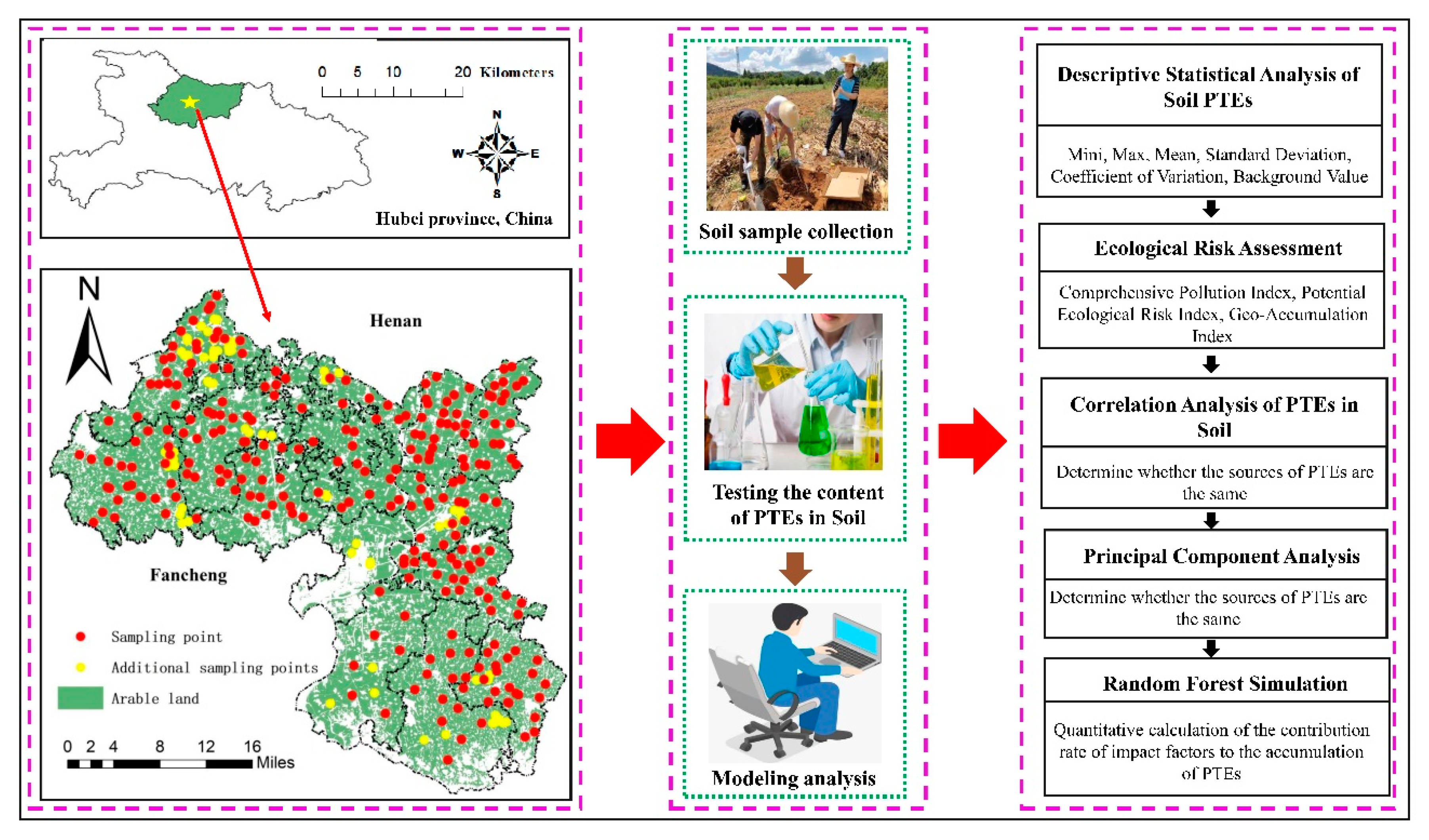
2.1. Study Location

Xiangzhou belongs to Hubei Province, China. The research region has a subtropical humid monsoon continental climate with an annual average temperature of 15.3–5.8 °C and annual average precipitation of 800–900 mm [12]. The agricultural land is 202,807.25 hectares, accounting for 82.22% of the total land area. The main soil type is yellow-brown soil with 1.05–3.39% soil organic matter; these kinds of soils are rich in organic matter since they are usually found in the tropical areas [13]. The yellowish-brown iron oxide goethite forms comparatively stable complexes, the enrichment of goethite would then cause a yellowing of the top soil [14]. Moreover, the soil pH was recorded as 4.8–7.1, and 1.5–1.6 g/cm³ was the soil bulk density [15].

The four main industries in Xiangzhou include agricultural product processing, textile and clothing, equipment manufacturing, and automobile parts. This district has abundant agricultural resources, and modern agriculture that has distinctive characteristics with a strong comprehensive agricultural production capacity. The main food crops are rice, wheat, and corn. Xiangzhou has a convenient and open location for transportation, the whole district has superior railway, highway, and aviation facilities as well as huge potential water transport conditions. The population density in Xiangzhou is 406 persons/km², thus it is a densely populated area.

2.2. Sample Analysis

Sampling points (at a depth of 0–20 cm) were arranged in the light of the distribution of arable land in Xiangzhou, 50 m apart from each other, covering the entire cultivated area via a designed grid system. From a total of 326 sample points, 255 samples were collected in August 2020, and 71 samples were taken around suspected pollution sources (livestock farm, mining areas, etc.) in September 2020. Of these, 79 sample points were in paddy fields, and 247 sample points were on irrigated land and dry land. The samples were evenly distributed in the cultivated land, and each sampling point represented an area of about 8–10 km². The points were carefully designed—after considering the difficulty of sampling, the pollution sources around the sampling points, and whether they were evenly distributed, the points were arranged on drawings.

Surface soil samples were collected from cultivated land in August 2020. First, debris was removed from the soil sample sampling site and placed into a clean cloth bag. After air-drying at room temperature and further removing plant roots, rocks, insects, and other debris, a rubber hammer was used to break the pieces and pass them through a 20-mesh (0.90 mm) nylon sieve. The samples were evenly mixed and divided into quarters and then sent to the laboratory for analysis and testing. The soil’s physical and chemical properties—such as contents of potentially toxic elements, organic matter content, bulk density, available potassium, available phosphorus, and pH—were analyzed and tested in the laboratory, in strict accordance with the Ecological Geochemical Evaluation Sample Analysis Method and Technology Requirements DD 2005-03 and Regional Geochemical Sample Analysis DZ/T 0279-2016, which required control accuracy [16].

The pH of the soil was gauged with a 0.01 mol/L calcium chloride (CaCl₂) solution (soil-to-liquid ratio of 1:5 mixed) for 30 min, then kept still for 1 h and measured with a pH meter [17]. The pretreated sample (1 g) was exactly weighed into a polytetrafluoroethylene receptacle, to which 20 mL of 0.005 mol/L diethylene triaminepentaacetic acid (DTPA), 0.01 mol/L calcium chloride (CaCl₂), and 0.1 mol/L triethylamine (TEA) were subjoined, and then sealed with microwave chemistry equipment created in the United States. The reaction equipment, namely a MARS5 microwave digester (Guangzhou, China), was used to implement digestion and dissolution. The microwave digestion parameters were power 1600 W, 120 °C for 2 min; 150 °C for 10 min; and 180 °C for 20 min. Following the completion of digestion, samples were handled at 150 °C to drive away the residual acid until only a small amount remained, and the sample was conveyed to a 10 mL measuring flask, in which the digestion canister was washed with a 1% (volume fraction) nitric acid solution, the measuring flask was integrated, diluted to the mark, and mixed well for use [18].

For determination of soil pH, the selective ion electrode means was adopted. To survey and evaluate the total content of Pb and Cr, plasma spectrometry was adopted—this method has many advantages, such as high detection efficiency and accuracy and simple and easy usage procedure [19]. The flameless atomic absorption method was adopted for total Cd content determination. The benefit of graphite furnace atomic absorption spectrometry is that the graphite furnace can improve the extent of element atomization [20]. For determination of the total content of As and Hg, atomic fluorescence spectrometry was used. The certified reference sample for the quality command (GSS-8) was used to guarantee the result’s accurateness. Analytical exactness for sample replicates was ±10% with measurement uncertainties between the determined values and the certified values of <5% [21].

2.3. Environmental Variables

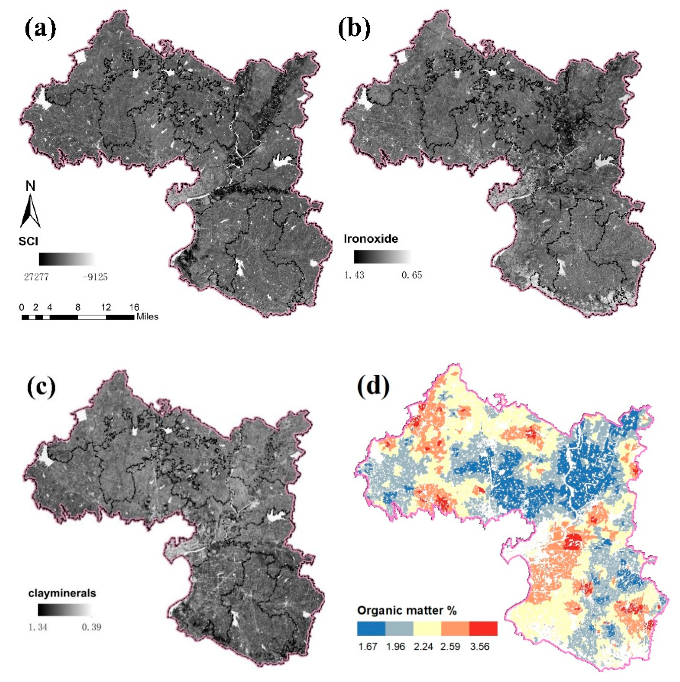
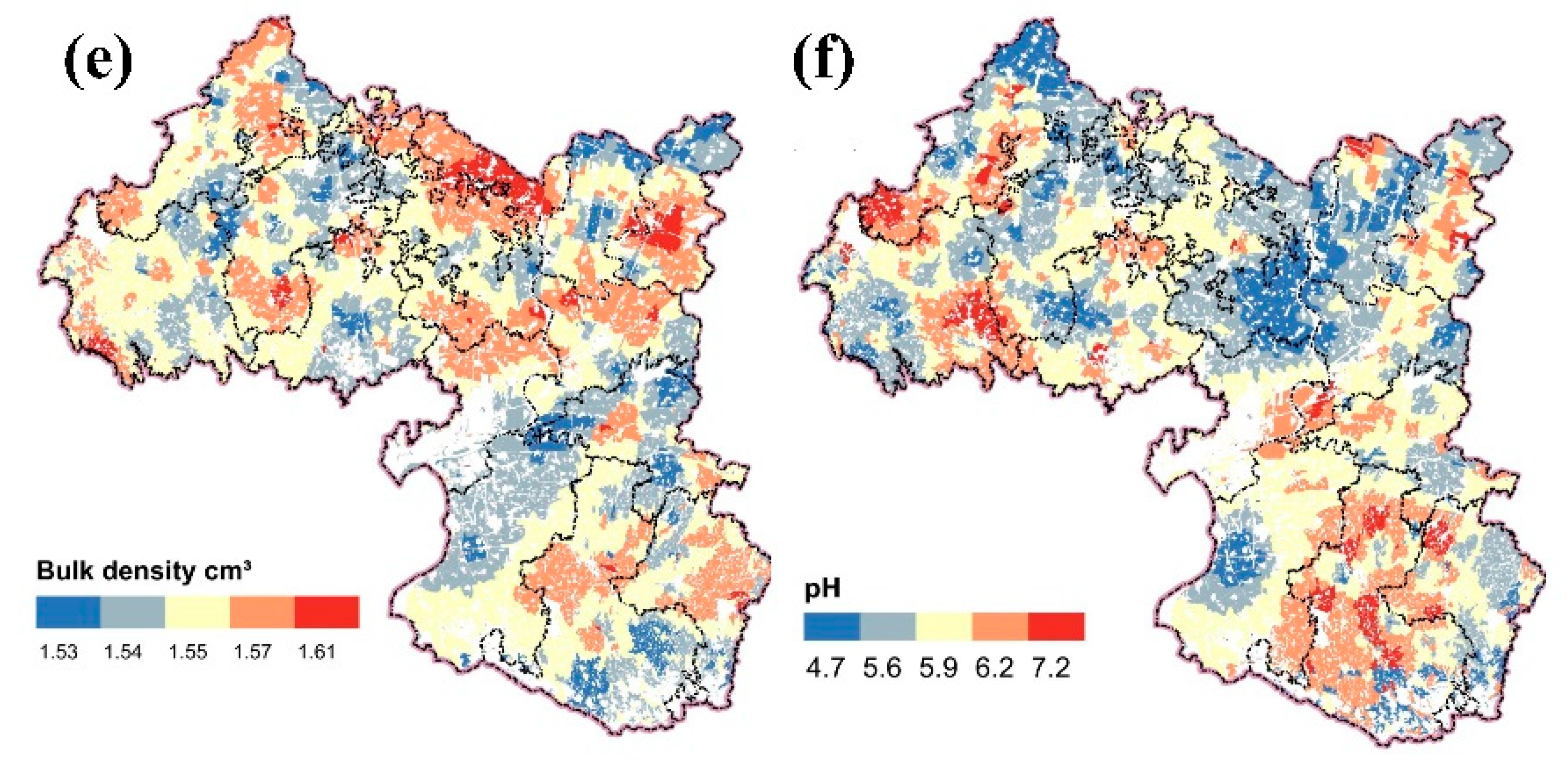
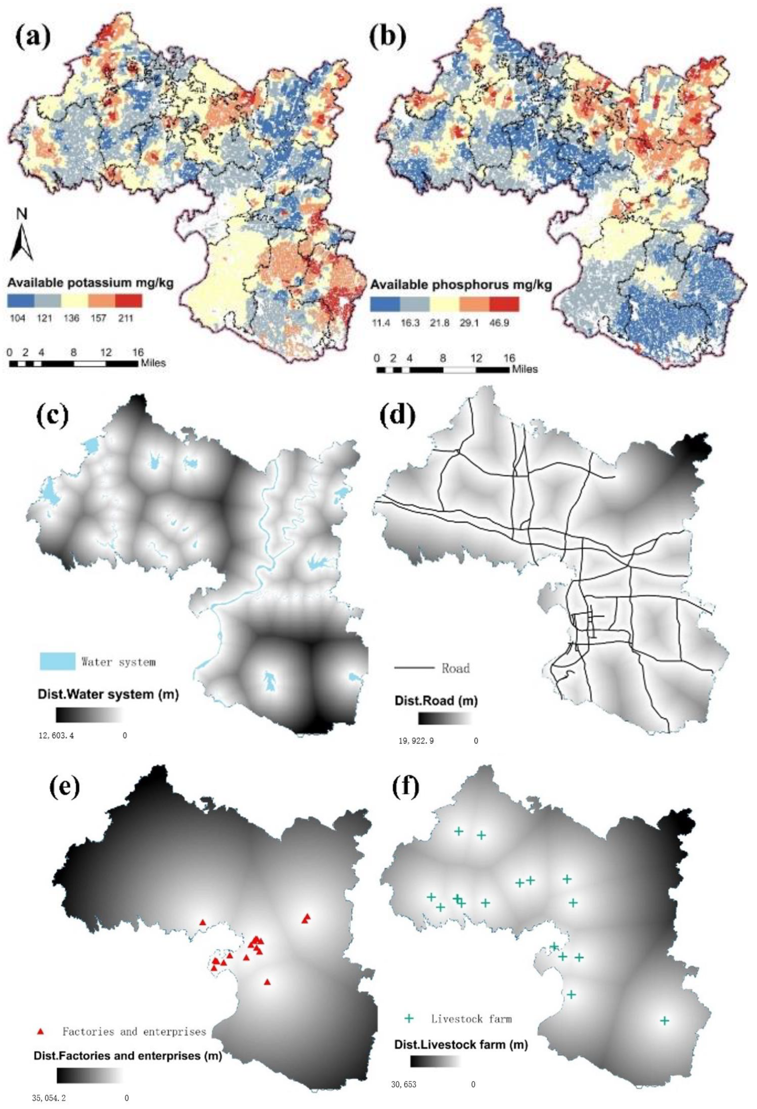
2.3.1. Natural Factors

Landsat 8 data in August 2020 was used in this study. Prior to image analysis, we performed remote sensing image preprocessing in ENVI software. The soil color index (SCI) reflects the content of humus in the soil, Figure 1a, humus can absorb potentially toxic elements in the soil [22], preventing possible harm caused by their continuous diffusion in the soil and thereby reducing pollution [23]. Iron oxide is an important component of soil, yellow soil contains more hydrated iron oxide. Red soil forms iron bauxite under the action of desiliconization and aluminum enrichment [24], Figure 1b. Clay minerals reflect the distribution and content of clay in the study area, Figure 1c; its adsorption has an important influence on the content of trace elements in the soil [25]. Carboxyl, hydroxyl, carbonyl, phenolic hydroxyl, methoxy, aldehyde, ether, amine, etc. are the most important functional groups of organic matter. It is these large number of functional groups that produce high reactivity, so they can interact with metals in the environment, Figure 1d. Frequent interactions of ions influence the content of potentially toxic elements in the soil [26]. Soil bulk density is an important indicator reflecting soil porosity and permeability, Figure 1e. Potential toxic elements will dissolve, precipitate, complex, and adsorb in the soil [27]. The pH value of the soil affects the effectiveness of potentially toxic elements, Figure 1f. Studies have found that when the pH value in the soil is higher, the reactivity of potentially toxic elements will be significantly reduced, making it difficult for them to be absorbed by plants [28].

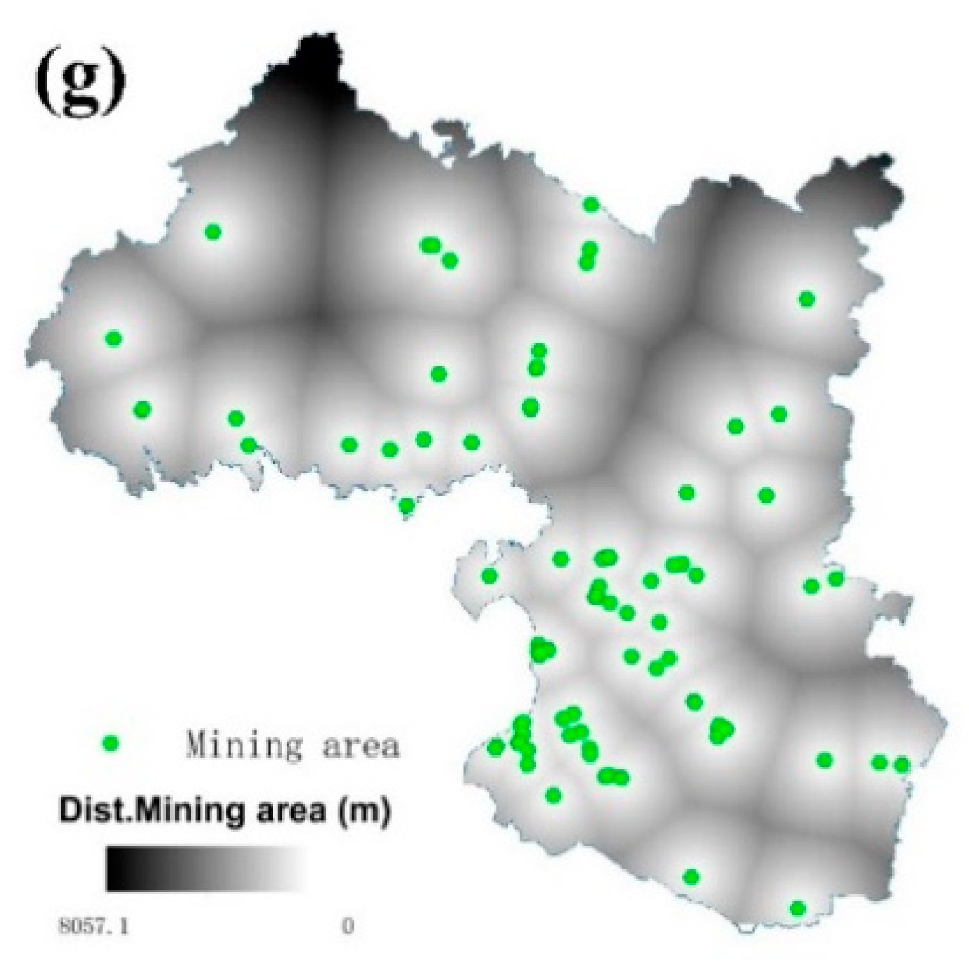
2.3.2. Artificial Factors

The available phosphorus and potassium can reflect the cumulative impact of artificial fertilization on the levels of potentially toxic elements in soil, Figure 2a,b. The water system, roads, industrial enterprises, livestock farms, and mining areas were analyzed in ArcGIS software using the Euclidean distance to obtain the sample point, close to the water system and construction land, Figure 2c–g. The distances between them can illustrate the influence of human conducts on the soil environment, such as transportation, irrigation, and artificial breeding [29].

2.4. Methodology

2.4.1. Analytical Framework

A research framework with the association of multivariate statistical analysis, ecological risk assessment, correlation analysis, principal component analysis, and random forest model was built using five main steps: statistical summary, correlation analysis, principal component identification, source dedication calculation, and effect procedure analysis of important factors. Through statistical summary, the concentrations of each potentially toxic element in the study area would be revealed. Through ecological risk assessment calculation, the risk assessment integrates data from ecological risk assessment models, toxicology, and soil pollution research to assess the risks and harms that pollutants pose to environment [30]. Through correlation analysis and principal component analysis, in IBM SPSS Statistics 19 software, the main pollution sources could be determined for the study area. Then through random forest simulation, detailed sources’ contribution ratio could be acquired, and the key environmental variables would be selected to indicate the effect procedure of artificial and natural indicators on potentially toxic elements in soil.

Therefore, the effect contribution, effect factors, and effect procedure of artificial activities on potentially toxic elements contents in the soil of the study area could be indicated via the combined framework of the correlation analysis and principal component analysis and the random forest model. The models require lots of data for superior simulation manifestation. Numerous number and variety of data of this research could sustain the achievement of excellent model simulation representation. The primary procedures applied in this research are illustrated in Figure 3.

2.4.2. Ecological Risk Assessment

(1)

Comprehensive Pollution Index

The revised formulae for calculating the comprehensive pollution index are given in Equations (1) and (2) [31]:

$$P_i=C_i/S_i$$

(1)

$$P=\sqrt{\left(P_{imax}^2+P_{iave}^2\right)/2}$$

(2)

where $P_i$ is the single potentially toxic element pollution index, $C_i$ is the actual potentially toxic element content of the sample (mg/kg), $S_i$ is the soil pollution risk screening value of agricultural land (mg/kg), $P_{imax}$ is the max of potentially toxic element pollution index, and $P_{iave}$ is the average of potentially toxic element pollution index, as shown in

Table 1. The soil pollution risk screening value of agricultural land (mg/kg).

Element		Risk Screening Value
		pH ≤ 5.5	5.5 < pH ≤ 6.5	6.5 < pH ≤ 7.5	pH > 7.5
Cd	Paddy field	0.3	0.4	0.6	0.8
	Irrigated land, dry land	0.3	0.3	0.3	0.6
Hg	Paddy field	0.5	0.5	0.6	1.0
	Irrigated land, dry land	1.3	1.8	2.4	3.4
As	Paddy field	30	30	25	20
	Irrigated land, dry land	40	40	30	25
Pb	Paddy field	80	100	140	240
	Irrigated land, dry land	70	90	120	170
Cr	Paddy field	250	250	300	350
	Irrigated land, dry land	150	150	200	250

.

The soil was divided into five levels according to values of the comprehensive pollution index, as shown in

Table 2. The grading principle of the synthesis pollution index ($P$ ).

Level	Comprehensive Pollution Index	Comprehensive Pollution Degree
1	≤0.7	Safety
2	0.7–1.0	Cordon
3	1.0–2.0	Light pollution
4	2.0–3.0	Moderately polluted
5	>3.0	Heavy pollution

[32]. It should be considered that the index evaluation method is a weighted multifactor environmental quality index that considers the maximum value and is easily affected by this maximum value [33].

$P_{imax}$ is the highest potentially toxic element pollution index of the sample, $P_{iave}$ is the average potentially toxic element pollution index of the sample, and $P$ is the comprehensive potentially toxic element pollution index.

(2)

Potential Ecological Risk Index

We calculated the widely used ecological risk index to evaluate the ecological risk of potentially toxic elements in cultivated soils of Xiangzhou [34]. The potentially toxic elements’ potential ecological risk index method considers not only the biological toxicity of potentially toxic elements but also the comprehensive combination of multiple pollutants [35]. Potential ecological risk is widely used, which adopts a toxic-response factor for a given substance and, thus, can be used to assess the synthesized contamination risk to an ecological system [36]. The calculations are as in Equations (3) and (4) [37]:

$$E_i=T_i{F}_i=T_i\frac{C_i}{B_i}$$

(3)

$$RI={\displaystyle \sum }{E}_i$$

(4)

where $E_i$ is a single potentially toxic element risk factor, and $T_i$ is a single potentially toxic element toxicity response factor. With reference to the relevant literature, the T values of the five potentially toxic elements were 30, 40, 10, 5, and 2, respectively. $F_i$ is a single potentially toxic element pollution factor, $C_i$ is the actual content of potentially toxic elements in the sample (mg/kg), $B_i$ is the background value of potentially toxic elements in the region (mg/kg), and $RI$ is the sum of risk factors for the potentially toxic elements. The pollution levels and their thresholds are as shown in

Table 3. Classifying the standards of the potential ecological risk index and pollution degree of potentially toxic elements.

Level	Potential Ecological Risk Index	Degree of Risk	Level	Comprehensive Potential Ecological Risk Index	Degree of Risk
1	≤40	Low potential risk	1	≤150	Minor ecological hazard
2	40–80	Medium potential risk	2	150–300	Moderate ecological hazard
3	80–160	High potential ecological risk	3	300–600	Strong ecological hazard
4	160–320	High potential risk	4	>600	Very strong ecological hazard
5	>320	Very high potential risk	-	-	-

.

(3)

Geo-Accumulation Index

The geo-accumulation index was used for assessing the potentially toxic elements’ contamination of farmland soil due to the comprehensive influence of anthropogenic pollution factors, geochemical background values, and natural diagenesis factors that cause the background values to change [38].

The earth accumulation index is calculated as in Equation (5) [39]:

$$I_{geo}={\log }_2\left(\frac{C_i}{k{B}_i}\right)$$

(5)

where $I_{geo}$ is the geo-accumulation index, $C_i$ is the content of element i in the sediment (mg/kg), $B_i$ is the potentially toxic element background value of element i in the area (mg/kg), and $k$ considers that diagenesis may produce potentially toxic elements. The coefficient for the change in the background value is generally 1.5. No pollution ($I_{geo}$ ≤ 0) indicates no pollution, 0 < $I_{geo}$ ≤ 1 indicates no-to-moderate pollution, 1 < $I_{geo}$ ≤ 2 indicates moderate pollution, 2 <$I_{geo}$ ≤ 3 indicates moderate-to-severe pollution, 3 < $I_{geo}$ ≤ 4 indicates serious pollution, and 4 < $I_{geo}$ ≤ 5 indicates extreme pollution.

2.4.3. Random Forest Modeling

To indicate the effect procedure of artificial and natural factors on potentially toxic elements in soil, a random forest model is a non-linear, non-parametric pattern proposed by Breiman [40]. The random forest model comprises many decision trees, and the dataset is recursively divided into increasingly homogeneous subsets regarding the response variable [41]. All prediction sets are examined at each split to decide which prediction sets and which result of the prediction sets best subdivides the dataset [42]. Each tree is trained by stochastically selecting a set of variables. The selecting technology is defined as bootstrap sampling. This technology could make the random forest model less prone to overfitting [43].

The random forest package that was used is from R Studio software (https://www.rstudio.com). The important parameters of the random forest model are ntree, which determines lots of decision trees, and mtry, which is the number of distinct variables used at each node [44]. Random forest could quantify the scale of the source’s influence on the contamination of the environment soil, this technique has high accuracy, and there is no longer a need to premeditate overfitting. It is an important tool used for solving source pollution sharing calculations and can effectively deal with missing data; therefore, it is extremely suitable for researching the sources of potentially toxic elements in soil [45].

The random forest package in the statistical software R program (version 3.6.3) was used. The setting of mtry is often the square root of the number of variables (p); in this study it was 4, and the parameter ntree was set to 1000 [46].

3. Results and Discussion

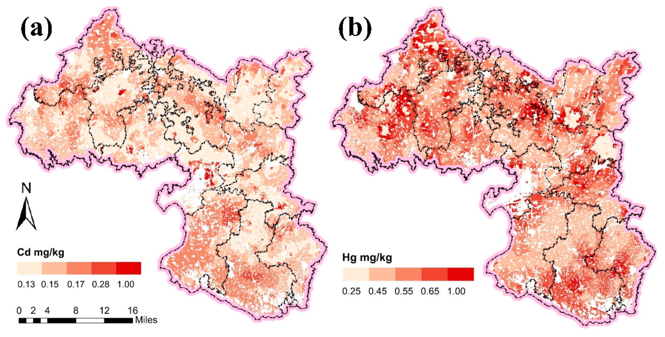
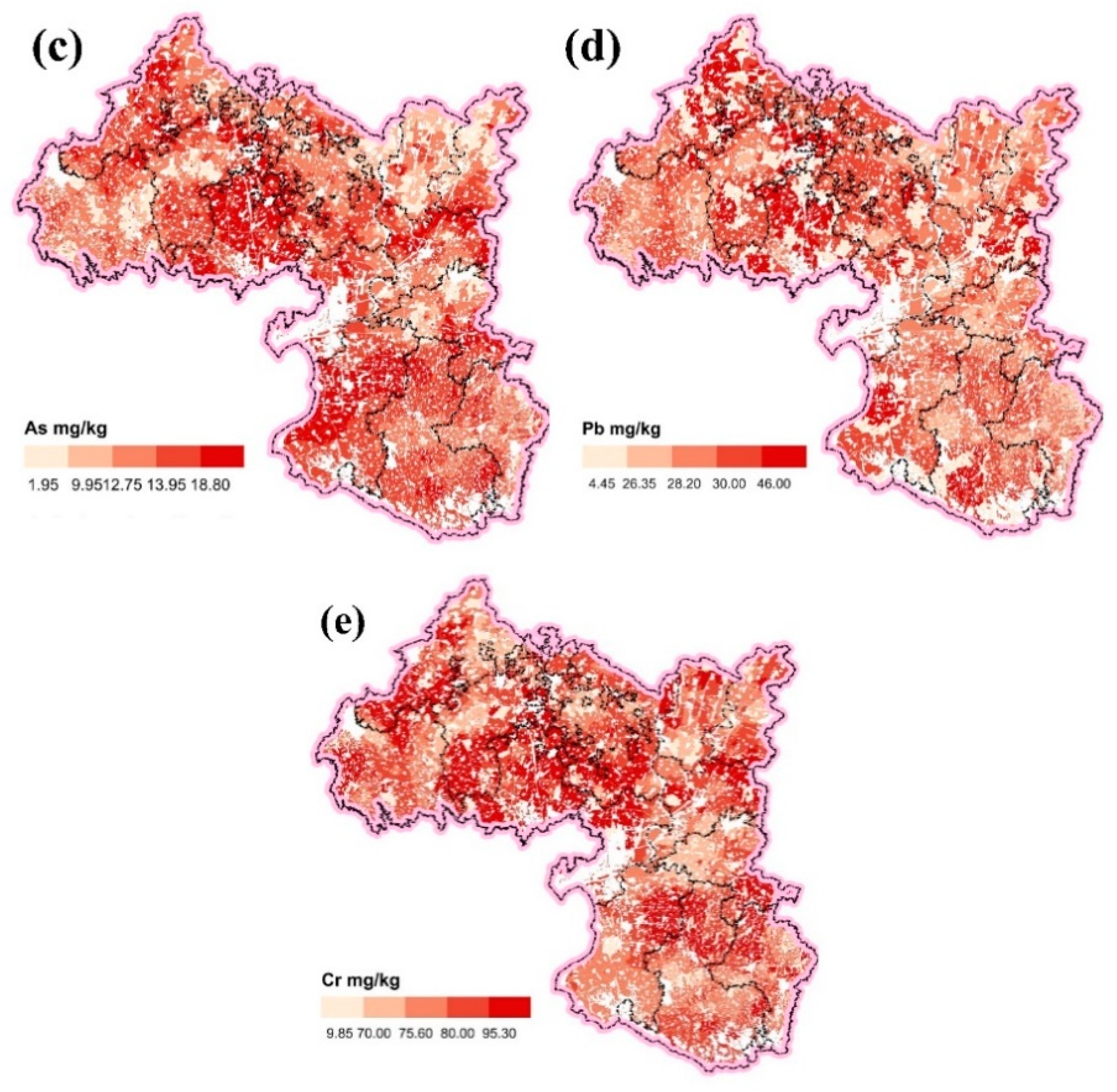
3.1. Spatial Distribution of Potentially Toxic Elements in Soil

To analyze the spatial distribution characteristics of the potentially toxic element soil content in the study area, the inverse distance weighting method was used in In ArcGIS software to draw the spatial distribution maps of the five potentially toxic elements, and it does not require the data to be normally distributed [47]. As shown in Figure 4, the spatial distribution of Cd is centered on the central old city, the Cd content in paddy fields near the northern waters of the study area and dry land near the hills and mountains in the south was higher than that in other areas; the Hg distribution is high in the surroundings and low in the middle, which presented a “basin” type distribution. The spatial distributions of As, Pb, and Cr are similar, all being high in the middle and lower in the surroundings.

3.2. Descriptive Statistical Analysis of Soil Potentially Toxic Elements

The descriptive statistical results of potentially toxic elements soil contents in the study area (

Table 4. The summary statistics of the soil potentially toxic elements concentrations for 326 points in Xiangzhou.

Element	Minimum	Maximum	Mean	Standard Deviation	Coefficient of Variation	Background Value
						Hubei, China	Jiangsu, China	South Iran [50]	European Mediterranean Area [51]
Cd (mg/kg)	0.06	0.28	0.14	0.03	21.43%	0.17	0.12	0.17	0.3
Hg (mg/kg)	0.02	0.5	0.05	0.05	100.00%	0.08	-	-	-
As (mg/kg)	6.54	19.8	12.33	2.55	20.68%	12.3	10.0	7.65	-
Pb (mg/kg)	20.1	47.1	28.39	3.94	13.88%	26.7	26.2	10.8	23.0
Cr (mg/kg)	52.9	96.7	75.21	8.91	11.85%	86.0	77.8-	74.5	27.0
pH	8.23	4.20	5.74	0.92	0.16%	-
Available potassium (mg/kg)	46.90	4.70	17.08	8.49	0.50%	-
Bulk density (cm3)	1.61	1.49	1.55	0.02	0.01%	-
Organic matter (%)	3.39	1.05	1.97	0.40	0.02%	-
Available phosphorus (mg/kg)	46.90	4.70	17.08	8.49	0.50%	-
Soil color index (SCI)	15,971.00	−1038.00	5377.78	1886.50	0.35%	-
Iron oxide	1.04	0.89	0.96	0.02	0.03%	-
Clay minerals	1.20	1.05	1.12	0.02	0.02%	-

), showed that the average contents of potentially toxic elements were 0.14 mg/kg (Cd), 0.05 mg/kg (Hg), 12.33 mg/kg (As), 28.39 mg/kg (Pb), and 75.21 mg/kg (Cr), respectively. The results compared with target values of neighboring regions and neighboring countries for Cd, As, Pb, and Cr showed mild pollution.

The average accumulation rate (mean/background value of Hubei [48]) for As and Pb were 1.01 and 1.06, respectively, and the research area was confronted with contamination caused by As and Pb. The ratio of the standard deviation to the average value is the coefficient of variation [49]. A descending order of the of the potentially toxic elements is: Hg (100%) > Cd (21.43%) > As (20.68%) > Pb (13.88%) > Cr (11.85%). The concentration of Hg ranged from 0.02 to 0.5 mg/kg, varied greatly, and the coefficient of variation was beyond 100%. Compared with the four other potentially toxic elements, Hg in the research area was extremely uneven, perhaps anthropogenic activity was the reason for the differentiation.

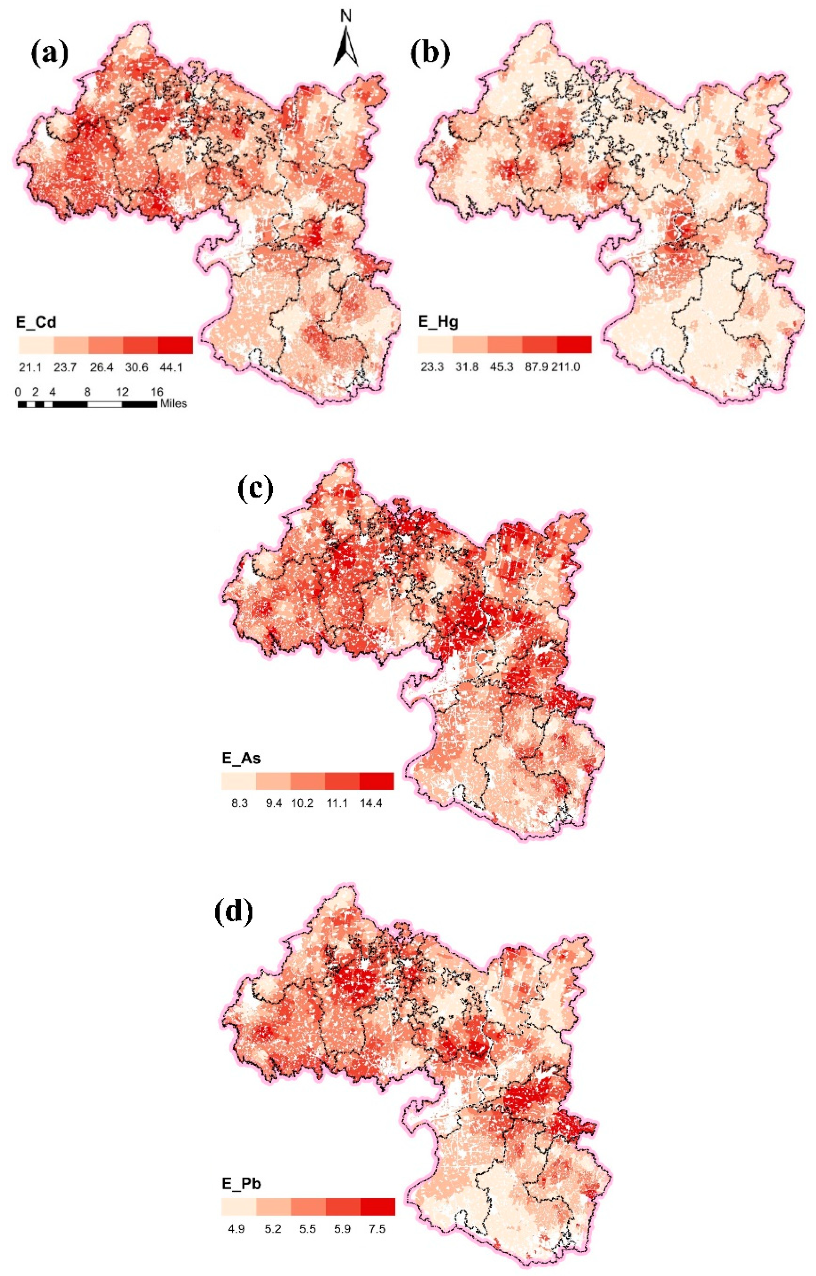
3.3. Ecological Risk Assessment Results

3.3.1. Comprehensive Pollution Index

According to the evaluation of the comprehensive pollution index, in paddy fields, dry land, and water-irrigated fields with a pH less than 5.5, Cd was within the range of the warning threshold, and the other elements were within safe levels. In paddy fields (

Table 5. The results for evaluation of comprehensive pollution index (paddy fields).

pH	Cd	Hg	As	Pb	Cr
<5.5	0.73	0.42	0.50	0.40	0.34
5.5–6.5	0.38	0.11	0.47	0.30	0.34
6.5–7.5	0.34	0.14	0.59	0.23	0.27
>7.5	0.21	0.45	0.54	0.10	0.19
Ave	0.42	0.28	0.53	0.26	0.29

), the degree of pollution in the surface soil collected from different plots due to the different toxic elements was of the order As (0.53) > Cd (0.42) > Cr (0.29) > Hg (0.28) > Pb (0.26). In dry land and irrigated land (

Table 6. The results for evaluation of comprehensive pollution index (dry land and water-irrigated fields).

pH	Cd	Hg	As	Pb	Cr
<5.5	0.71	0.41	0.39	0.53	0.57
5.5–6.5	0.64	0.07	0.36	0.35	0.55
6.5–7.5	0.60	0.12	0.48	0.32	0.41
>7.5	0.27	0.03	0.66	0.19	0.34
Ave	0.56	0.16	0.47	0.35	0.47

), this order was Cd (0.56) > As (0.47) = Cr (0.47) > Pb (0.35) > Hg (0.16).

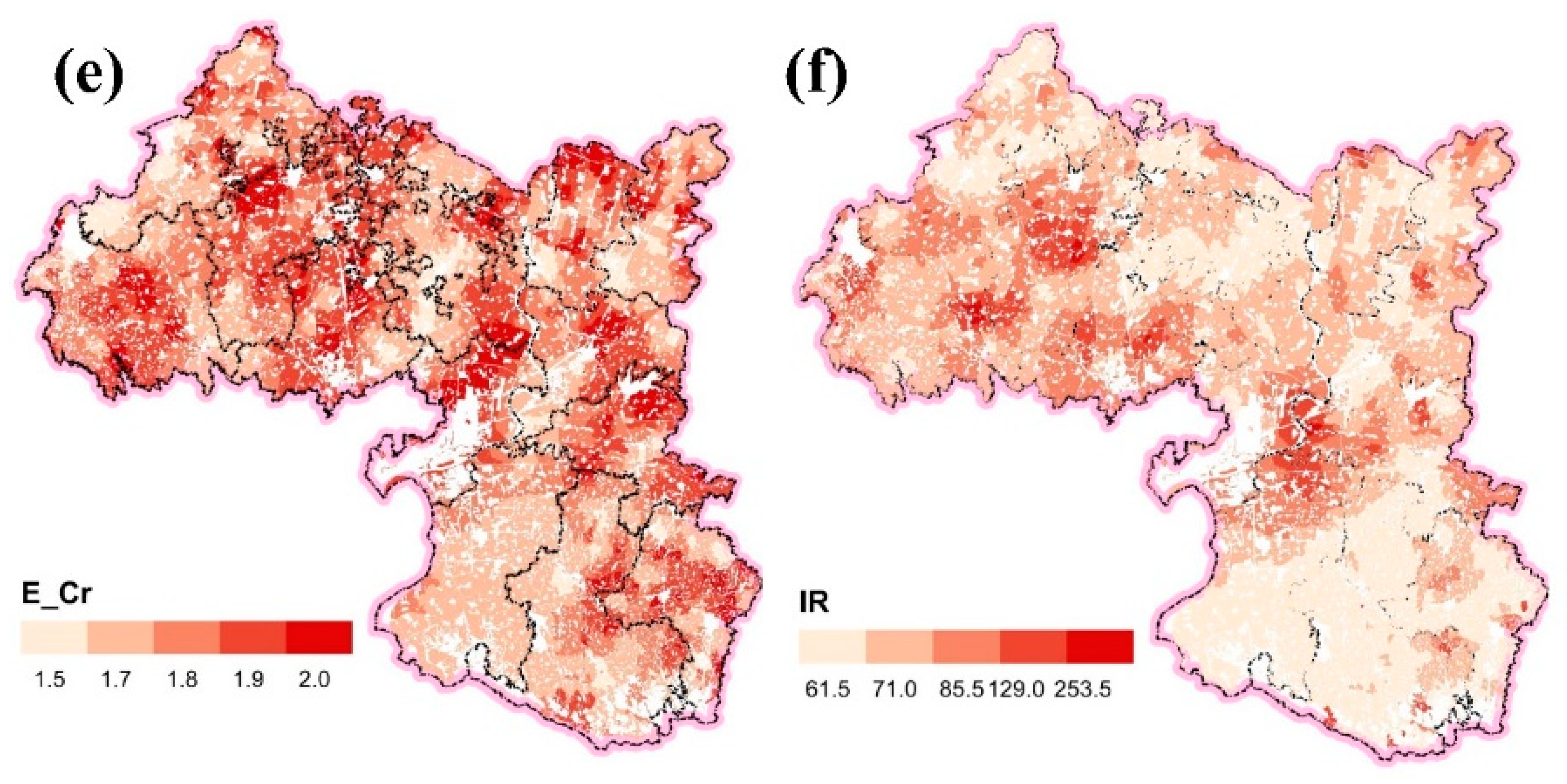
3.3.2. Potential Ecological Risk Index

The outcomes for the assessment of potential ecological risk due to pollution of soil with potentially toxic elements in the study area (

Table 7. The evaluation results of the potential ecological risk index.

	Statistical	Cd	Hg	As	Pb	Cr	$\mathbf{R}\mathbf{I}$
Potential ecological risk index statistics	Min	11.29	8.00	5.32	3.76	1.23	38.01
	Max	49.41	250	16.10	8.82	2.25	292.56
	Ave	24.48	25.83	10.02	5.32	1.75	67.39
Distribution of the potential ecological risk index (%)	≤40	98.77%	89.57%	100%	100%	100%	98.77%
	(40, 80]	1.23%	7.97%	-	-	-	1.23%
	(80, 160]	-	1.53%	-	-	-	-
	(160, 320]	-	0.92%	-	-	-	-
	>320	-		-	-	-	-

) showed that the average value of the potential ecological risk coefficient was of the order Hg (25.83) > Cd (24.48) > As (10.02)> Pb (5.32) > Cr (1.75). The ecological risk level due to As, Pb, and Cr was considered slight. Cd was mainly determined to pose a slight ecological risk, though in some cases, the risk was medium. The ecological risk for Hg was mainly slight and partly medium and strong.

RI is explicitly applied to infer quantitatively the ecological risk of potentially toxic elements. The average value of the potential ecological risk index was 67.39, of which the level of slight ecological risk accounted for 98.77%, indicating that the potentially toxic elements in the research region soil were mainly at the slight ecological risk standard.

Among the 326 sampling points, 4 sampling points were classified as 150 < $RI$ < 300, which indicates a moderate risk of ecological hazard; 4 sampling points were classified as 40 <$E_{Cd}$ < 80, which indicates a moderate degree of potential risk; 26 sampling points were categorized as 40 < $E_{\mathrm{Hg}}$ < 80, meaning a medium potential risk; 5 sampling points were categorized as 80 < $E_{\mathrm{Hg}}$ < 160, indicating a medium-to-high potential ecological risk; and 3 sampling points were at 160 < $E_{\mathrm{Hg}}$ < 320, indicating a high potential risk.

The contribution of various potentially toxic elements to the potential ecological risk index is equal to the ratio of its individual potential ecological risk modulus to the potential ecological risk index. The contribution rates of potentially toxic elements to the potential ecological risk index were 36.33% (Cd), 38.33% (Hg), 14.87% (As), 7.89% (Pb), and 2.60% (Cr), respectively, indicating that Cd and Hg were the main risk factors.

Inverse distance weighting interpolation was performed in ArcGIS software on the potential ecological risk coefficients of the sample points, as shown in Figure 5a–e, where the potential risk index of Cd is shown to be relatively high in the northeast, and the spatial distribution of the potential risk index of Hg is scattered from the center to the surroundings. The spatial distributions of the potential risk index of As, Pb, and Cr were relatively similar and successively decreasing, and these elements were all higher in the northeast and middle-east. The spatial distribution of the potential ecological hazard index is shown in Figure 5f. Strong–very strong ecological risk was found to be mainly distributed in the northeastern and central and western towns.

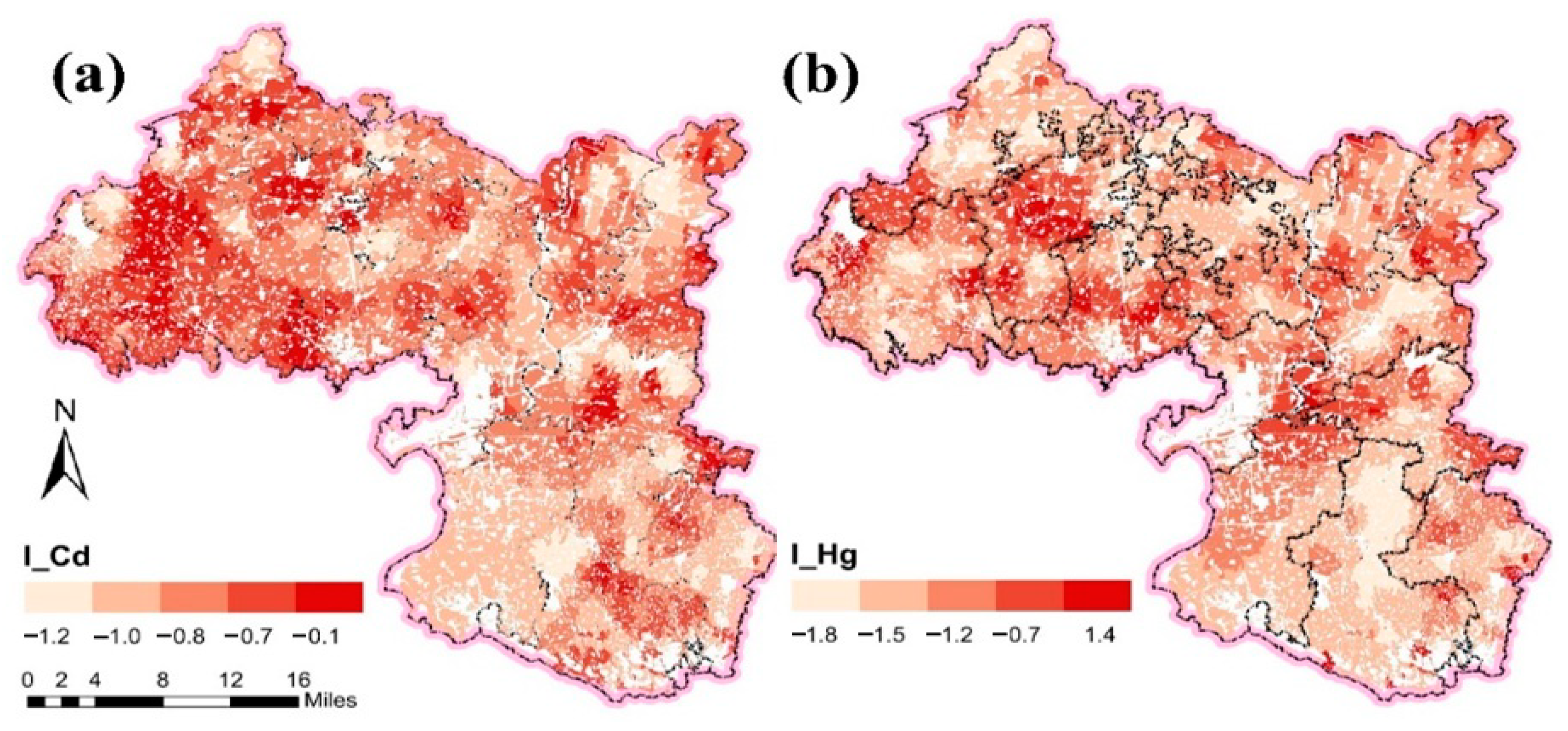
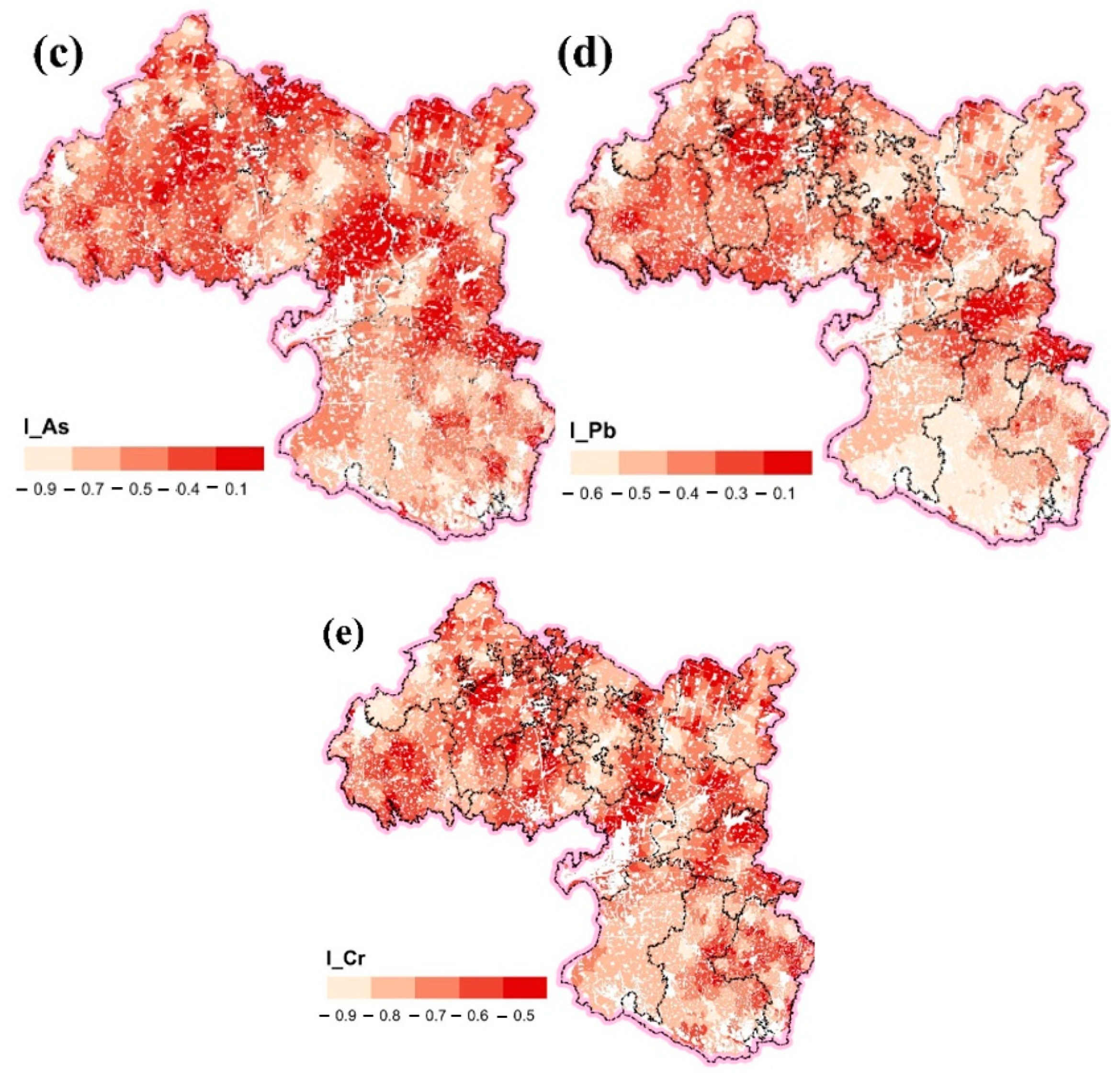
3.3.3. Geo-Accumulation Index Method

The evaluation results of the $I_{geo}$ (geo-accumulation index) of the five potentially toxic elements of the 326 sample points are shown in

Table 8. The evaluation results of the geo-accumulation index method.

${\mathit{I}}_{\mathit{g}\mathit{e}\mathit{o}}$	Cd	Hg	As	Pb	Cr
Min	−1.99	−2.91	−1.50	−0.99	−1.29
Max	0.13	2.06	0.10	0.23	−0.42
Ave	−0.91	−1.46	−0.62	−0.51	−0.79

. There is a certain degree of pollution in some areas. Among them, 0 < $I_{geo}$ < 1 for Cd, that is, there were 2 points with moderate pollution. For Hg, 8 points had 0 < $I_{geo}$ < 1, that is, moderate pollution; 1 < $I_{geo}$ < 2 for 3 points, which is a medium pollution degree; and 2 < $I_{geo}$ < 3 for 1 point, which is extreme pollution. For As, there was 1 point with 0 < $I_{geo}$ < 1, which is a moderate pollution degree. For Pb, 5 points were 0 <$I_{geo}$ < 1, which indicates a moderate pollution degree.

Figure 3 shows the inverse distance weighting of $I_{geo}$ in ArcGIS software. The high-value area of Cd is mainly concentrated in the northwest region, Figure 6a. The spatial distribution of the geo-accumulative index of Hg is scattered from the center to the surroundings and then decreases in sequence, Figure 6b. The spatial distributions of the potential risk index for As, Pb, and Cr were relatively similar, being higher in the northeast, central, and eastern regions, Figure 6c–e.

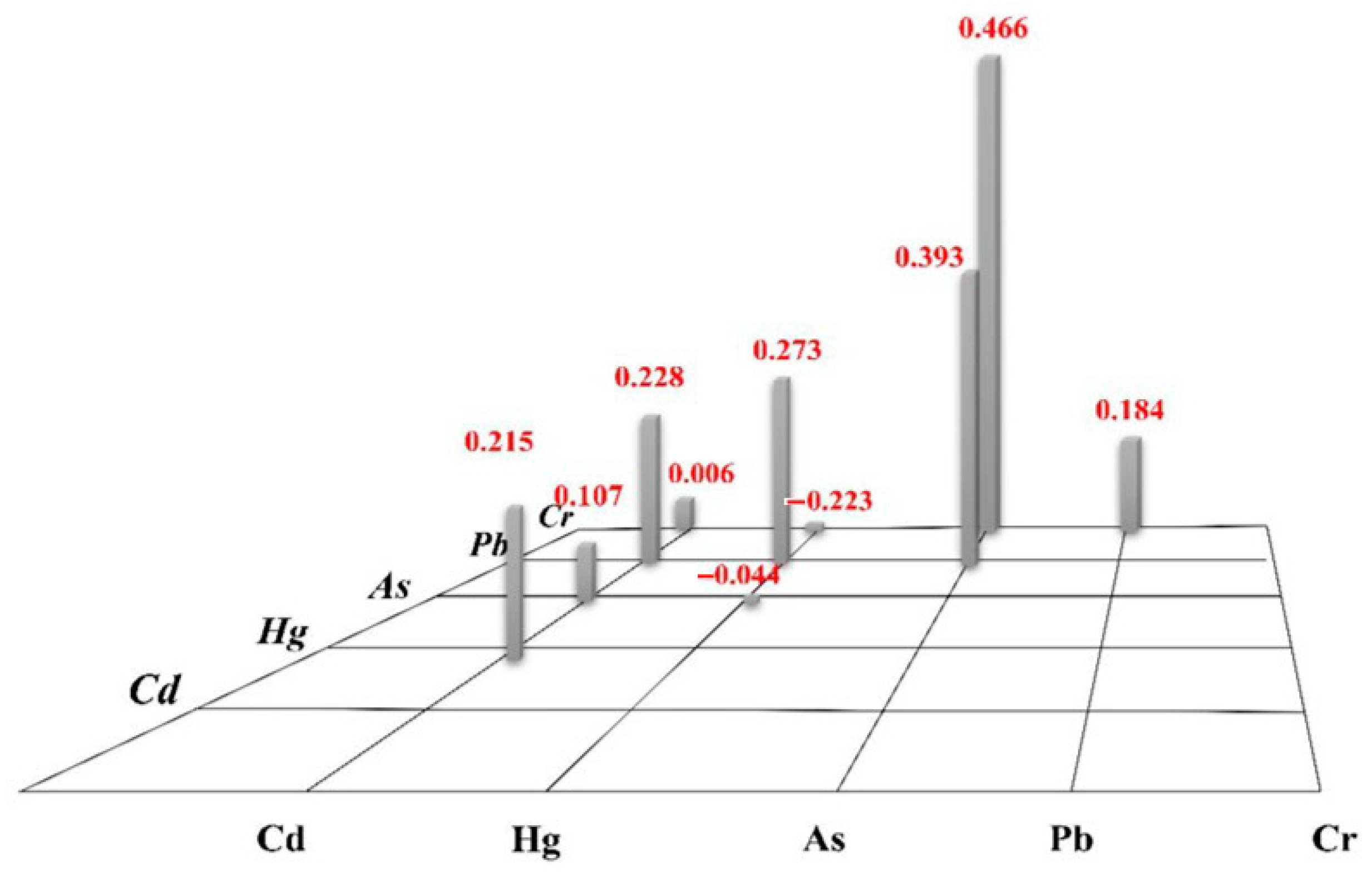
3.4. Correlation Analysis of Potentially Toxic Elements in Soil

Spearman correlation analysis was performed on the data of the five potentially toxic elements in 326 soil samples using SPSS 22 software (

Table 9. Correlation analysis of potentially toxic elements concentrations in research area.

Element	Cd	Hg	As	Pb	Cr
Cd	1.000
Hg	0.215 **	1.000
As	0.107	−0.044	1.000
Pb	0.228 **	0.273 **	0.393 **	1.000
Cr	0.006	−0.223 **	0.466 **	0.184 **	1.000

** Significantly correlated at the 0.01 level (bilateral).

and Figure 7), and was chosen because it does not require normality of variables. The correlations between As and Pb and between As and Cr were found to be 0.393 and 0.466, respectively, indicating a greater likelihood of having common sources. The correlations between Hg and Pb, Cd and Hg, and Pb and Cr were 0.273, 0.215, and 0.184, respectively, indicating that they may have a common source.

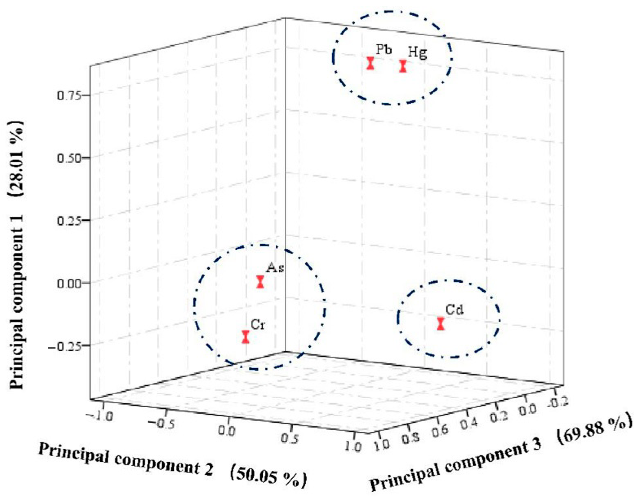
3.5. Principal Component Analysis

The Kaiser–Meyer–Olkin and Bartlett sphere test were carried out in SPSS software. The Kaiser–Meyer–Olkin was 0.528 > 0.5, and P was 0.0000. That is, the related feasibility of the Bartlett sphericity test was 0.0000 < 0.05; therefore, the specimen data can be subjected to principal component analysis.

The Kaiser standardized orthogonal rotation method was used for principal component analysis, as shown in

Table 10. The results of principal component analysis.

	Factor Load (Orthogonal Rotation)
Metals	Principal Component 1	Principal Component 2	Principal Component 3
Cd	−0.16	0.78	0.29
Hg	0.79	0.13	−0.01
As	0.05	0.06	0.91
Pb	0.79	−0.11	0.01
Cr	−0.28	−0.66	0.39
% Variance contribution rate	28.01	22.04	19.84
% Cumulative contribution rate	28.01	50.05	69.88

and Figure 8. The multivariate was reduced to three factors (the characteristic root was greater than one). The first three components illustrated 69.88% of the total variable variance. The main variables of the first main factor (which explained 28.01% of the total variance) included Hg and Pb, indicating that these two elements have a high degree of homology; the second main factor (the increase explained 22.04% of the total variance) included Cd; the main variables of the third main factor (an increase of 19.84%) were As and Cr.

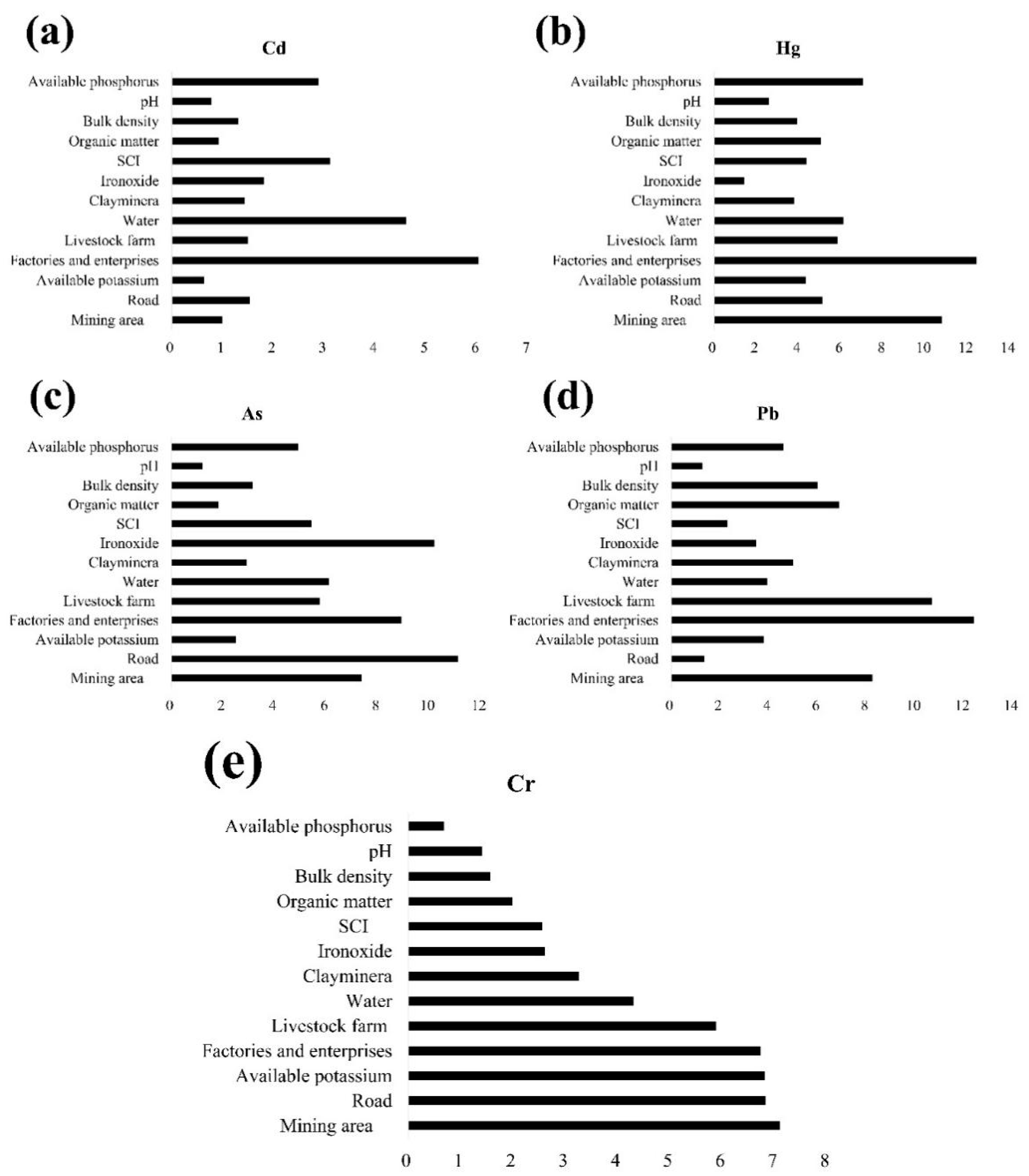
3.6. Random Forest Simulation

The random forest package in the statistical software R program (version 3.6.3) was used. The setting of mtry is often the square root of the number of variables (p); in this study it was 4, and the parameter ntree was set to 1000 [52].

In this research, the following means to using legacy data for training model was applied: the ratio of the training set (260 samples) and the validation set (66 samples) was set to 8:2, and the overall accuracy r² (correlation coefficient) of the models for potentially toxic elements was 93.35%, 95.88%, 94.11%, 93.95%, and 93.20%, respectively, indicating high accuracy. The results of the variable importance measure are listed in

Table 11. Results of the variable importance measure in Xiangzhou.

Variable Importance Measure	Cd	Hg	As	Pb	Cr
pH	0.79	2.58	1.19	1.27	1.41
Bulk density	1.31	3.93	3.15	5.99	1.57
Organic matter	0.93	5.06	1.82	6.89	1.99
Soil color index (SCI)	3.12	4.39	5.44	2.30	2.56
Iron oxide	1.81	1.43	10.21	3.47	2.61
Clay minerals	1.44	3.80	2.92	4.99	3.25
Available potassium	0.64	4.34	2.51	3.78	6.80
Available phosphorus	2.89	7.05	4.93	4.59	0.68
Water	4.61	6.12	6.11	3.94	4.30
Mining area	1	10.77	7.39	8.25	7.10
Factories and enterprises	6.03	12.41	8.94	12.40	6.73
Livestock farm	1.50	5.84	5.75	10.69	5.88
Road	1.53	5.12	11.11	1.35	6.83

.

As shown in Figure 9, the variable importance measure represents the weight of the anthropogenic influencing factors. The top four factors explaining Cd were factories and enterprises (6.03%) > water (4.61%) > soil color index (SCI) (3.12%) > available phosphorus (2.89%), Figure 9a. The top four factors explaining Hg were factories and enterprises (12.41%) > mining areas (10.77%) > available phosphorus (7.05%) > water (6.12%), Figure 9b. The top four factors explaining As were roads (11.11%) > iron oxide (10.21%) > factories and enterprises (8.94%) > mining areas (7.39%), Figure 9c. The top four factors explaining Pb were factories and enterprises (12.40%) > livestock farms (10.69%) > mining areas (8.25%) > organic matter (6.89%), Figure 9d. The top four factors explaining Cr were mining areas (7.10%) > roads (6.83%) > available potassium (6.80%) > factories and enterprises (6.73%), Figure 9e.

The random forest results showed that among the top four factors affecting Cd, factories and enterprises, agricultural irrigation, artificial fertilization, and road transportation were the most important factors, which demonstrated that the accumulation of Cd was primarily from human activities [53]. Potentially toxic elements from farm animals may enter the nearby agricultural land in the form of farm manure, once again verifying the accuracy of the results [54]. The long-term application of chemical fertilizers (such as phosphate fertilizer and potash fertilizer) in agricultural activities and farmland farming methods that use sewage containing a large amount of potentially toxic elements for irrigation will significantly increase the accumulation and contents of potentially toxic elements in farmland soil [55].

Correlation analysis and principal component analysis both demonstrated that the origin consistency of Hg and Pb was high. In the random forest analysis, the top four artificial factors affecting their distribution were found to be factories, enterprises, mining areas, and livestock farms. Industrial and agricultural production lead to mercury contamination in the environmental soil [56]. In this study, Hg was more affected by human factors, whereas Pb was affected by the combined influence of human activities and natural accumulation.

The results of various analyses in this study illustrated that the origins of As and Cr were highly consistent. The random forest regression model showed that roads, factories, and water system distance from mining areas and farms were the common cumulative sources, indicating that the accumulation of these two potentially toxic elements was strongly affected by human activities. In the light of a previous research, industrial manufacturing and processing, mining industry, metal smelting and transportation in mining region, and livestock fertilizer from farm can lead to the enrichment of As and Cr [57]. Industrial activities and transportation also affect the levels of potentially toxic elements in regional dust fall, further affecting their contents in the surrounding soil [58]. As and Cr are exhausted into the environment with the exhaust gas of cars, while the wearing out of vehicle parts during transportation cause As and Cr to pollute the environmental soil along with dust and dirt in the atmosphere [59].

4. Conclusions

These properties of potentially toxic elements not only worsen the quality of the soil circumstance and change the ecological function of the soil but also directly or indirectly affect human health [60]. Carrying out environment risk assessment research can provide a basis for the scientific evaluation of potentially toxic element pollution of soil, pollution treatment, and reasonable soil redevelopment [61].

The three calculation methods used in this paper all showed that the soil was Cr-pollution-free (low pollution); however, ecological risks of As, and Pb still exist, with obvious differences [62]. Cd and Hg were the main risk factors, with imminent health and environment risks.

Long-term industrial pollution, mineral mining and processing, exhaust emissions from transportation, the application of manure from farms as fertilizer, and sewage irrigation are the main anthropogenic sources of toxic elements pollution in the cultivated soils [63]. In response to the pollution results from this investigation, in addition to continuing to control the production and processing of polluted gases and waste emissions in factories, it is also necessary to control the excessive introduction of potentially toxic elements from livestock manure into farmland soil environments to avoid further pollution, and potentially toxic elements in feces should be processed before being discharged into soil [64]. Inorganic passivating agents can be added to the feces, such as: fly ash, calcium bentonite, phosphate rock, or zeolite, which can effectively adsorb potentially toxic elements, thereby reducing their biological effectiveness [65].

References

1. Md Anawar, H.; Chowdhury, R. Remediation of Polluted River Water by Biological, Chemical, Ecological and Engineering Processes. Sustainability 2020, 12, 7017. [Google Scholar] [CrossRef]
2. Yang, Y.; Christakos, G.; Guo, M.; Xiao, L.; Huang, W. Space-time quantitative source apportionment of soil heavy metal concentration increments. Environ. Pollut. 2017, 223, 560–566. [Google Scholar] [CrossRef] [PubMed]
3. Ke, X.; Gui, S.; Huang, H.; Zhang, H.; Wang, C.; Guo, W. Ecological risk assessment and source identification for heavy metals in surface sediment from the Liaohe River protected area, China. Chemosphere 2017, 175, 473–481. [Google Scholar] [CrossRef] [PubMed]
4. Nanos, N.; Martín, J.A.R. Multiscale analysis of heavy metal contents in soils: Spatial variability in the Duero river basin (Spain). Geoderma 2012, 189, 554–562. [Google Scholar] [CrossRef]
5. Hou, D.; Li, F. Complexities surrounding China’s soil action plan. Land Degrad. 2017, 28, 2315–2320. [Google Scholar] [CrossRef] [Green Version]
6. Chen, Z.; Shi, D. Spatial Structure Characteristics of Slope Farmland Quality in Plateau Mountain Area: A Case Study of Yunnan Province, China. Sustainability 2020, 12, 7230. [Google Scholar] [CrossRef]
7. Bandara, N.; Hettiarachchi, H.; Jensen, E.; Binoy, T.H. Upcycling Potential of Industrial Waste in Soil Stabilization: Use of Kiln Dust and Fly Ash to Improve Weak Pavement Subgrades Encountered in Michigan, USA. Sustainability 2020, 12, 7226. [Google Scholar] [CrossRef]
8. Kamta, F.N.; Schilling, J.; Scheffran, J. Insecurity, Resource Scarcity, and Migration to Camps of Internally Displaced Persons in Northeast Nigeria. Sustainability 2020, 12, 6830. [Google Scholar] [CrossRef]
9. Breiman, L. Random forests. Mach. Learn. 2001, 45, 5–32. [Google Scholar] [CrossRef] [Green Version]
10. Oves, M.; Khan, M.S.; Zaidi, A.; Ahmad, E. Soil contamination, nutritive value, and human health risk assessment of heavy metals: An overview. Toxic. Heavy Met. Legum. Bioremediat. 2012, 1, 1–28. [Google Scholar]
11. Brtnický, M.; Pecina, V.; Baltazár, T.; Vašinová Galiová, M.; Baláková, L.; Bęś, A.; Radziemska, M. Environmental Impact Assessment of potentially toxic elements in Soils Near the Runway at the International Airport in Central Europe. Sustainability 2020, 12, 7224. [Google Scholar] [CrossRef]
12. Xiao, L.; Zhou, Y.; Huang, H.; Liu, Y.-J.; Li, K.; Li, M.-Y.; Tian, Y.; Wu, F. Application of Geostatistical Analysis and Random Forest for Source Analysis and Human Health Risk Assessment of potentially toxic elements (PTEs) in Arable Land Soil. Int. Environ. Res. Public Health 2020, 17, 9296. [Google Scholar] [CrossRef] [PubMed]
13. Nehren, U.; Kirchner, A.; Heinrich, J. What do yellowish-brown soils and stone layers tell us about Late Quaternary landscape evolution and soil development in the humid tropics? A field study in the Serra dos Órgãos, Southeast Brazil. Catena 2016, 137, 173–190. [Google Scholar] [CrossRef]
14. Wrb I W G. World Reference Base for Soil Resources 2014 International Soil Classification System for Naming Soils and Creating Legends for Soil Maps[M]//World Reference Base for Soil Resources 2014. International Soil Classification System for Naming Soils and Creating Legends for Soil Maps. 2014. Available online: https://ec.europa.eu/jrc/en/printpdf/151713 (accessed on 26 December 2020).
15. Hodson, M.E. The need for sustainable soil remediation. Elements 2010, 6, 363–368. [Google Scholar] [CrossRef]
16. Soriano, H.; Maria, C. Environmental Risk Assessment of Soil Contamination. Environ. Risk Assess. Soil Contam. 2014. [Google Scholar] [CrossRef]
17. Adamo, P.; Iavazzo, P.; Albanese, S.; Agrelli, D.; de Vivo, B.; Lima, A. Bioavailability and soil-to-plant transfer factors as indicators of potentially toxic element contamination in agricultural soils. Sci. Total Environ. 2014, 500–501, 11–22. [Google Scholar] [CrossRef]
18. Mazurek, R.; Kowalska, J.; Gąsiorek, M.; Zadrożny, P.; Józefowska, A.; Zaleski, T.; Kępka, W.; Tymczuk, M.; Orłowska, K. Assessment of heavy metals contamination in surface layers of Roztocze National Park forest soils (SE Poland) by indices of pollution. Chemosphere 2017, 168, 839–850. [Google Scholar] [CrossRef]
19. Vareda, J.P.; Valente, A.J.; Duraes, L. Heavy metals in Iberian soils: Removal by current adsorbents/amendments and prospective for aerogels. Adv. Colloid Interface Sci. 2016, 237, 28–42. [Google Scholar] [CrossRef]
20. Chandrasekaran, A.; Ravisankar, R.; Harikrishnan, N.; Satapathy, K.K.; Prasad, M.V.R.; Kanagasabapathy, K.V. Multivariate statistical analysis of heavy metal concentration in soils of Yelagiri Hills, Tamilnadu, India-Spectroscopical approach. Spectrochim. Acta Part A Mol. Biomol. Spectrosc. 2015, 137, 589–600. [Google Scholar] [CrossRef]
21. Huo, Z.; Tian, J.; Wu, Y.; Ma, F. A Soil Environmental Quality Assessment Model Based on Data Fusion and Its Application in Hebei Province. Sustainability 2020, 12, 6804. [Google Scholar] [CrossRef]
22. Liu, H.; Yang, R.; Zhou, Z.; Huang, D. Regional Green Eco-Efficiency in China: Considering Energy Saving, Pollution Treatment, and External Environmental Heterogeneity. Sustainability 2020, 12, 7059. [Google Scholar] [CrossRef]
23. Arditsoglou, A.; Samara, C. Levels of total suspended particulate matter and major trace elements in Kosovo: A source identification and apportionment study. Chemosphere 2005, 59, 669–678. [Google Scholar] [CrossRef] [PubMed]
24. Buatmenard, P.; Chesselet, R. Variable influence of the atmospheric flux on the trace metal chemistry of oceanic suspended matter. Earth Planet. Sci. Lett. 1979, 42, 399–411. [Google Scholar] [CrossRef]
25. Burges, A.; Epelde, L.; Garbisu, C. Impact of repeated single-metal and multimetal pollution events on soil quality. Chemosphere 2015, 120, 8–15. [Google Scholar] [CrossRef]
26. Bzdusek, P.A.; Lu, J.; Christensen, E.R. PCB Congeners and Dechlorination in Sediments of Sheboygan River, Wisconsin, Determined by Matrix Factorization. Environ. Sci. Technol. 2006, 40, 120–129. [Google Scholar] [CrossRef]
27. Jiao, X.; Teng, Y.; Zhan, Y. Soil Heavy Metal Pollution and Risk Assessment in Shenyang Industrial District, Northeast China. PLoS ONE 2015, 10, e0127736. [Google Scholar] [CrossRef] [Green Version]
28. Yaylaliabanuz, G. Heavy metal contamination of surface soil around Gebze industrial area, Turkey. Microchem. J. 2011, 99, 82–92. [Google Scholar] [CrossRef]
29. Arik, F.; Yaldiz, T. Heavy Metal Determination and Pollution of the Soil and Plants of Southeast Tavşanlı (Kütahya, Turkey). Clean-Soil Air Water 2010, 38, 1017–1030. [Google Scholar] [CrossRef]
30. Comero, S.; Vaccaro, S.; Locoro, G. Characterization of the Danube River sediments using the PMF multivariate approach. Chemosphere 2014, 95, 329–335. [Google Scholar] [CrossRef]
31. Guney, M.; Zagury, G.J.; Dogan, N. Exposure assessment and risk characterization from trace elements following soil ingestion by children exposed to playgrounds, parks and picnic areas. Hazard. Mater. 2010, 182, 656–664. [Google Scholar] [CrossRef]
32. Jiménez-Ballesta, R.; García-Navarro, F.J.; Bravo, S.; Amoros, J.A.; Pérez de los Reyes, C.; Mejias, M. Environmental assessment of potential toxic elements contents in the inundated floodplain área of Tablas de Daimiel wetland (Spain). Environ. Geochem. Health 2017, 39, 1159–1177. [Google Scholar] [CrossRef] [PubMed]
33. Kara, M.; Dumanoglu, Y.; Altiok, H. Spatial distribution and source identification of trace elements in topsoil from heavily industrialized region, Aliaga, Turkey. Environ. Monit. Assess. 2014, 186, 6017–6038. [Google Scholar] [CrossRef] [PubMed]
34. Kim, M.; Deshpande, S.R.; Crist, K.C. Source apportionment of fine particulate matter (PM 2.5) at a rural Ohio River Valley site. Atmos. Environ. 2007, 41, 9231–9243. [Google Scholar] [CrossRef]
35. Roy, M.; Mcdonald, L.M. Metal Uptake in Plants and Health Risk Assessments in Metal-Contaminated Smelter Soils. Land Degrad. Dev. 2015, 26, 785–792. [Google Scholar] [CrossRef]
36. Salonen, V.; Korkkaniemi, K. Influence of parent sediments on the concentration of heavy metals in urban and suburban soils in Turku, Finland. Appl. Geochem. 2007, 22, 906–918. [Google Scholar] [CrossRef]
37. Schaefer, K.; Einax, J.W. Source Apportionment and Geostatistics: An Outstanding Combination for Describing Metals Distribution in Soil. Clean-Soil Air Water 2016, 44, 877–884. [Google Scholar] [CrossRef]
38. Vaccaro, S.; Sobiecka, E.; Contini, S.; Locoro, G.; Free, G.; Gawlik, B.M. The application of positive matrix factorization in the analysis, characterisation and detection of contaminated soils. Chemosphere 2007, 69, 1055–1063. [Google Scholar] [CrossRef]
39. Fei, J.-C.; Min, X.-B.; Wang, Z.-X.; Pang, Z.-H.; Liang, Y.-J.; Ke, Y. Health and ecological risk assessment of heavy metals pollution in an antimony mining region: A case study from South China. Environ. Sci. Pollut. Res. Int. 2017, 24, 27573–27586. [Google Scholar] [CrossRef]
40. Hu, B.; Xue, J.; Zhou, Y.; Shao, S.; Fu, Z.; Li, Y.; Chen, S.; Chen, L.; Shi, Z. Modelling bioaccumulation of heavy metals in soil-crop ecosystems and identifying its controlling factors using machine learning. Environ. Pollut. 2020, 262, 114308. [Google Scholar] [CrossRef]
41. Xu, R.; Sun, X.; Han, F.; Li, B.; Xiao, E.; Xiao, T.; Yang, Z.; Sun, W. Impacts of antimony and arsenic co-contamination on the river sedimentary microbial community in an antimony-contaminated river. Sci. Total Environ. 2020, 713, 136451. [Google Scholar] [CrossRef]
42. Zhou, X.Y.; Wang, X.R. Impact of industrial activities on heavy metal contamination in soils in three major urban agglomerations of China. J. Clean. Prod. 2019, 230, 1–10. [Google Scholar] [CrossRef]
43. El Azhari, A.; Rhoujjati, A.; El Hachimi, M.L.; Ambrosi, J.-P. Pollution and ecological risk assessment of heavy metals in the soil-plant system and the sediment-water column around a former Pb/Zn-mining area in NE Morocco. Ecotoxicol. Environ. Saf. 2017, 144, 464–474. [Google Scholar] [CrossRef] [PubMed]
44. Yi, Y.; Yang, Z.; Zhang, S. Ecological risk assessment of heavy metals in sediment and human health risk assessment of heavy metals in fishes in the middle and lower reaches of the Yangtze River basin. Environ. Pollut. 2011, 159, 2575–2585. [Google Scholar] [CrossRef] [PubMed]
45. He, X.; Song, X.; Pang, Y.; Li, Y.; Chen, B.; Feng, Z. Distribution, sources, and ecological risk assessment of SVOCs in surface sediments from Guan River Estuary, China. Environ. Monit. Assess. 2014, 186, 4001. [Google Scholar] [CrossRef] [PubMed]
46. Kadi, M.W. “Soil Pollution Hazardous to Environment”: A case study on the chemical composition and correlation to automobile traffic of the roadside soil of Jeddah city, Saudi Arabia. J. Hazard. Mater. 2009, 168, 1280–1283. [Google Scholar] [CrossRef]
47. Mukherjee, A.B.; Zevenhoven, R.; Brodersen, J. Mercury in waste in the European Union: Sources, disposal methods and risks. Resour. Conserv. Recycl. 2004, 42, 155–182. [Google Scholar] [CrossRef] [Green Version]
48. Geng, F.; Cai, C.; Tie, X. Analysis of VOC emissions using PCA/APCS receptor model at city of Shanghai, China. J. Atmos. Chem. 2009, 62, 229–247. [Google Scholar] [CrossRef]
49. Josse, J.; Husson, F. Selecting the number of components in principal component analysis using cross-validation approximations. Comput. Stat. Data Anal. 2012, 56, 1869–1879. [Google Scholar] [CrossRef]
50. Moghtaderi, H.; Shakeri, T.; Andrés Rodríguez-Seijo, A. Potentially Toxic Element Content in Arid Agricultural Soils in South Iran. Agronomy 2020, 10, 564. [Google Scholar] [CrossRef]
51. Davis, H.T.; Aelion, C.M.; Mcdermott, S. Identifying natural and anthropogenic sources of metals in urban and rural soils using GIS-based data, PCA, and spatial interpolation. Environ. Pollut. 2009, 157, 2378–2385. [Google Scholar] [CrossRef] [Green Version]
52. Jimenez-Ballesta, R.; Bravo, S.; Amorós, J.A.; Pérez-De-Los-Reyes, C.; García-Giménez, R.; Higueras, P.; Garcia-Navarro, F. Mineralogical and Geochemical Nature of Calcareous Vineyard Soils from Alcubillas (La Mancha, Central Spain). Int. Environ. Res. Public Health 2020, 17, 6229. [Google Scholar] [CrossRef] [PubMed]
53. Jiang, Y.; Chao, S.; Liu, J.; Yang, Y.; Chen, Y.; Zhang, A.; Cao, H. Source apportionment and health risk assessment of heavy metals in soil for a township in Jiangsu Province, China. Chemosphere 2017, 168, 1658–1668. [Google Scholar] [CrossRef] [PubMed]
54. Fernandez, S.; Cotosyanez, T.R.; Rocapardinas, J. Geographically weighted principal components analysis to assess diffuse pollution sources of soil heavy metal: Application to rough mountain areas in Northwest Spain. Geoderma 2018, 311, 120–129. [Google Scholar] [CrossRef] [Green Version]
55. Johansson, C.; Norman, M.; Burman, L. Road traffic emission factors for heavy metals. Atmos. Environ. 2009, 43, 4681–4688. [Google Scholar] [CrossRef]
56. Oconnor, D.; Hou, D.; Ok, Y.S. Sustainable in situ remediation of recalcitrant organic pollutants in groundwater with controlled release materials: A review. J. Control. Release 2018, 283, 200–213. [Google Scholar] [CrossRef] [PubMed]
57. Peng, T.; Oconnor, D.; Zhao, B. Spatial distribution of lead contamination in soil and equipment dust at children’s playgrounds in Beijing, China. Environ. Pollut. 2019, 245, 363–370. [Google Scholar] [CrossRef]
58. Yu, X.; Li, H.; Doluschitz, R. Towards Sustainable Management of Mineral Fertilizers in China: An Integrative Analysis and Review. Sustainability 2020, 12, 7028. [Google Scholar] [CrossRef]
59. Xie, W.; Peng, C.; Wang, H.; Chen, W. Health Risk Assessment of Trace Metals in Various Environmental Media, Crops and Human Hair from a Mining Affected Area. Int. Environ. Res. Public Health 2017, 14, 1595. [Google Scholar] [CrossRef] [Green Version]
60. Young, F.J.; Hammer, R.D. Defining Geographic Soil Bodies by Landscape Position, Soil Taxonomy, and Cluster Analysis. Soil Sci. Soc. Am. J. 2000, 64, 989–998. [Google Scholar] [CrossRef] [Green Version]
61. Zhang, P.; Hou, D.; Oconnor, D. Green and Size-Specific Synthesis of Stable Fe–Cu Oxides as Earth-Abundant Adsorbents for Malachite Green Removal. ACS Sustain. Chem. Eng. 2018, 6, 9229–9236. [Google Scholar] [CrossRef]
62. Maanan, M.; Saddik, M.; Maanan, M.; Chaibi, M.; Assobhei, O.; Zourarah, B. Environmental and ecological risk assessment of heavy metals in sediments of Nador lagoon, Morocco. Ecol. Indic. 2015, 48, 616–626. [Google Scholar] [CrossRef]
63. Li, Q.; Gu, F.; Zhou, Y.; Xu, T.; Wang, L.; Zuo, Q.; Xiao, L.; Liu, J.; Tian, Y. Changes in the Impacts of Topographic Factors, Soil Texture, and Cropping Systems on Topsoil Chemical Properties in the Mountainous Areas of the Subtropical Monsoon Region from 2007 to 2017: A Case Study in Hefeng, China. Int. Environ. Res. Public Health 2021, 18, 832. [Google Scholar] [CrossRef]
64. Pekey, H.; Dogan, G. Application of positive matrix factorisation for the source apportionment of heavy metals in sediments: A comparison with aprevious factor analysis study. Microchem. J. 2013, 106, 233–237. [Google Scholar] [CrossRef]
65. Micó, C.; Recatalá, L.; Peris, M.; Sánchez, J. Assessing heavy metal sources in agricultural soils of an European Mediterranean area by multivariate analysis. Chemosphere 2006, 65, 863–872. [Google Scholar] [CrossRef] [PubMed]
Figure 1. Natural accumulation in the study area. The spatial distribution of (a) soil color index (SCI), (b) iron oxide, (c) clay minerals, (d) organic matter, (e) bulk density, and (f) pH.
Sustainability 13 01214 g001aSustainability 13 01214 g001b
Figure 2. Human activities in the study area. The spatial distribution of (a) available potassium, (b) available phosphorus, (c) water systems, (d) roads, (e)f and enterprises, (f) livestock farms, and (g) mining areas.
Sustainability 13 01214 g002aSustainability 13 01214 g002b
Figure 3. Schematic diagram of research ideas.
Sustainability 13 01214 g003
Figure 4. Spatial distribution of potentially toxic elements in soil in the study area. (a) Spatial distribution of Cd; (b) spatial distribution of Hg; (c) spatial distribution of As; (d) spatial distribution of Pb; (e) spatial distribution of Cr.
Sustainability 13 01214 g004aSustainability 13 01214 g004b
Figure 5. The spatial distribution of the potential ecological risk coefficient in the research region shown individually for (a) Cd, (b) Hg, (c) As, (d) Pb, (e) Cr and (f) IR.
Sustainability 13 01214 g005aSustainability 13 01214 g005b
Figure 6. The spatial distribution of I g e o (geo-accumulation index) in the study area shown individually for (a) Cd, (b) Hg, (c) As, (d) Pb, and (e) Cr.
Sustainability 13 01214 g006aSustainability 13 01214 g006b
Figure 7. Correlation analysis of potentially toxic element concentrations in research area.
Sustainability 13 01214 g007
Figure 8. The results of principal component analysis.
Sustainability 13 01214 g008
Figure 9. Plots of the variable importance measures in Xiangzhou. Variable importance measure results for (a) Cd, (b) Hg, (c) As, (d) Pb, and (e) Cr.
Sustainability 13 01214 g009