
The Inland Container Transportation Problem with Separation Mode Considering Carbon Dioxide Emissions


Transportation Management College, Dalian Maritime University, Dalian 116026, China
*
Author to whom correspondence should be addressed.
Sustainability 2021, 13(3), 1573; https://0-doi-org.brum.beds.ac.uk/10.3390/su13031573
Submission received: 29 December 2020
/
Revised: 20 January 2021
/
Accepted: 28 January 2021
/
Published: 2 February 2021
(This article belongs to the Special Issue Dynamic Trans-Sino-Europe Transport Networks and Their Impacts on Sustainable Goals (UNSDGs))
Abstract
:This paper investigates the Inland Container Transportation (ICT) problem with carbon dioxide emissions. The separation mode that the tractor and semi-trailer could be detached and it permits multitasking to reduce fuel and carbon emission costs. A mixed-integer programming model with Full-Empty container integration has been built. An improved ant colony optimization with two-dimensional variable matrix encoding and Infeasible-Arc filtration strategy has been proposed. Numerical experiments with different scales and characteristics are simulated and validated in order to demonstrate the effectiveness of the proposed algorithm. The comparison result indicates the excellent stability for our approach with different task characteristic distribution.
1. Introduction
Containerization has become an essential part of regional and international markets, accompanying economic globalization development. In the meantime, this overwhelming transport requirement has further exposed the negative ecological hazards [1]. As the previous research indicates, freight transportation activities are one of the fundamental strengths influencing the expansion of carbon emitters [2,3,4,5]. With the freight network oriented toward sustainability, strengthening the efficiency of transport organization structure and promoting positive attitudes towards low-carbon technologies are becoming significant challenges and topics. When comparing to overland transportation equipment, maritime transportation of freight is the relatively ecological friendly alternative. Nonetheless, ocean vessel inability to provide door to door transportation services and inland transportation of shipping containers must be performed by highway vehicles, increasing the resulting emissions. Therefore, it is essential to investigate the carbon dioxide emissions from inland container transportation (ICT), which could be described as an inland container transportation problem with carbon emissions management (ICT-CEM).
An ICT-CEM problem is typically organized, as follows: a local area near a terminal having a significant number of containerization freight demand and numerous empty container and vehicle resources in hand. In addition, the transportation demand from customers is further split into inbound and outbound trips. However, the majority of customers do not possess empty containers. Thus, the transportation demand might be subdivided into four interrelated tasks: Delivery Full Container (DFC), Pickup Empty Container (PEC), Delivery Empty Container (DEC), and Pickup Full Container (PFC). For the decision-makers, a crucial problem in constructing a low-carbon sustainable network is to choose the appropriate vehicle scheduling solutions with a lower fuel cost and carbon footprint. Recent research has shown that the drop-and-pull transportation mode has a dramatic improvement for energy-saving and emission-reduction [6]. Consequently, it would be beneficial to adopt a drop-and-pull mode in the ICT problem.
In the inland container dispatch process, empty container repositioning is a high-profile pain point. Unlike the loaded containers, the movement of empty containers does not directly benefit revenue stream [7], but with a potential impact on freight network performance. In the meantime, it produces a large number of unprofitable transportation costs and carbon emissions. The separation mode between trucks and containers would improve the utilization of trucks and decrease the waiting time for loading/unloading. Meanwhile, empty containers and full containers can transform mutually and collaborative transport under a single transportation cycle and mitigate the secondary transportation cost and carbon emission.
On the basis of the above analysis, we investigate the ICT problem with the tractor and semi-container separation mode to reduce the fuel cost and carbon pollution. A mixed-integer programming model of tractor routing is presented. For the ICT with separation mode, two types of the task as interrelated operations in which empty containers and loaded containers can mutually transform and collaboratively transport under a single transportation cycle. Meanwhile, the two freight tasks could be assigned to different tractors. When combined with temporal constraints for tractor transportations and container loading/unloading, the central challenge is to generate a feasible solution. Therefore, an improved ant colony optimization (ACO) with two-dimensional variable matrix encoding and an Infeasible-arc filtration strategy is designed. Finally, numerical experiments with different scales and characteristics are given in order to show the advantages of separation mode and computing performance of the modified ACO algorithm.
The remainder of the paper is organized, as follows: Section 2 reviews three categories of research related to ICT, vehicle separation mode, and carbon emission in ICT, respectively. In Section 3, we define the transportation task and link-arc in the ICT problem. Section 4 shows the search procedures of the improved ACO algorithm with the brand-new encode method and select strategy. The computational results on experiments of various distributions are shown in Section 5. Finally, Section 6 gives the conclusion and future work of this paper.
2. Literature Review
We categorize the relevant research into three distinct classifications: the ICT problem, the vehicle routing problem with separation mode and the carbon emission minimization in container transportation problem.
2.1. The ICT Problem
Zhang et al. [8] first proposed the ICT problem, and formulated it as an asymmetric multi-traveling salesman problem with time windows (m-TSPTW). Furthermore, these authors proposed two heuristic algorithms to solve this problem. Extended research achievement of Multi-depots and Multi-terminals [9,10,11], flexible tasks [12], Multi-size container [13], Foldable container [14], and Multi-resource constraints [15] have investigated in their follow-up studies. Since the ICT problem was proposed, it has attracted widespread attention from scholars [16,17,18,19,20,21]. Sebastian Sterzik [22] integrated the reposition of the full and empty container in harbor hinterland areas, where empty containers resource could interchange among cooperating freight companies. The numerical experiments included 75 transportation requests and showed the huge potential of container sharing. Song [23] and Shan [24] studied this issue based on a robust mathematical model and a determined-activities-on-vertex (DAOV) graph, respectively. Afterwards, they both used the branch-and-price algorithm to provide an accurate solution. Daham et al. [25] focused on the unbalanced ICT problem with import-oriented port area and considered the multi-size container issue based on the pairing of containers in drayage transportation (PCDT) model. The core technology of their model was to combine freight orders, and it was more efficient than the traditional vehicle scheduling model on large-scale instances.
The ICT problem can be defined as a variant of the pickup and delivery problem (PDP) with time window, which has been proven to be NP-hard. Therefore, the ICT problem can also be regarded as an NP-hard problem [26], and numerous heuristic algorithms have been presented. Sebastian Sterzikn and Herbert Kopfer [27] proposed a Tabu Search (TS) Heuristics with a modified savings algorithm to assign this problem, small-scale and realistic-sized test case studies were performed in order to demonstrate the effectiveness of their algorithm. Ji S and Luo R [28] considered the multi-objective of minimum total transportation cost and maximum flow time situation; a hybrid heuristic algorithm that is based on multi-object local search was proposed to search the Pareto dominance. Vidović M et al. [29] addressed multi-size container scenario and designed an improved variable neighborhood search (VNS) heuristic.
In summary, experiments in previous research have shown that the commercial solver (e.g., CPLEX) only guarantees the ability to obtain an accurate and reliable solution within a reasonable time (about 3 h) up to 20 orders. Therefore, the study of heuristic algorithms had arisen as a significant role. Although ICT could be regarded as an extension of the vehicle scheduling problem, the solution structures were dramatically different. The central process of a heuristic algorithm in ICT was encoding a constructive procedure, decoding rule, and solution update strategy.
2.2. Vehicle Routing Problem with Separation Mode
The separation mode is a novel mode of operation to container repositioning. Typically, the container transportation problem with a separation mode could be subdivided into the truck&trailer routing problem (TTRP) and tractor&semi-trailer routing problem (TSRP).
Chao first proposed the standard mathematical model and benchmark instances of TTRP in 2002 [30]; afterwards, it was investigated by Tan et al. [31], Lin et al. [32], Villegas et al. [33,34], etc., and they presented various intelligent optimization algorithms. TTRP was widely used in North America and European Union countries. In this problem, the vehicle can separate into a truck and trailer, and the demand has been split into the two characteristics: (a) Truck Customer: the location that expected to perform the truck process alone; (b) Trailer Customer: the location that is expected to perform the truck process with the trailer or alone.
The truck and trailer mode has been limited to traffic law restriction in China and several Asian governments; the tractor and semi-trailer mode was used in these countries. The TSRP is a branch research direction of TTRP, and the vehicle routes are pendulum tours among different customer locations and terminals. Lu et al. [35] focused on the multimodal transport two-echelon location-routing problem with consolidation (ME-2E-LRP-C), and proposed a hybrid differential evolution algorithm in order to solve the two-layer mixed integer linear problem (MILP) model. Yang et al. [36] studied a TSRP with uncertain empty-trailer tasks; the experimental results showed that empty-trailer transportation cost could reduce the average operating cost by 3.62% when compared to the original scheme.
In our research, empty/full container yard and inbound/outbound customers are served by several tractors and semi-trailer with containers. Different from TSRP mode, we allow overlap from different vehicles, which is empty and a full container task of a customer might be scheduled by two different vehicles. Xue et al. [37,38] examined the ICT problem under separation mode and designed a max-min ACO algorithm to solve large-scale problems. Caballini et al. [39] considered the cooperating of multiple trucks carries. Sun et al. [40] investigated Ro-ro shipping under the land–sea combined transportation problem, and proposed a new port-swap mode that is based on separation mode. The result revealed that the new operation mode is more efficient than the traditional ship-swap mode.
2.3. Carbon Emission Minimization in Container Transportation Problem
There is a tiny amount of research that introduced the ICT problem with carbon dioxide emission. Liao et al. [41] analyzed the carbon emission impact from the emerging port to existing ports. An activity-based emission model was proposed in order to estimate the empirical study of a Taipei port. The result demonstrated the advantage of the newly developed sea-lane. Jaehun Sim [42] estimated the carbon emissions for the container terminal. The experimental analysis showed that a majority of carbon pollution comprised from the container vessel maneuver process, the summation of a vessel at berth process, and container transport process were less than 2%, container load/unload and container pickup/delivery with 37% and 10% of responses, respectively. Shao hung Goh [43] investigated this problem again with foldable containers, which would balance the full and empty container tasks and reduce carbon pollution ratio. Hoen et al. [44] proposed an inventory model with carbon emission measurement methodology and considered the impact of different emission regulations. Fan et al. [45] proposed a hybrid heuristic approach to assign the carbon emissions under Truck Appointment System (TAS); a realistic-sized instance of China was reported. The experimental results showed that the TAS could reduce the carbon pollution ratio by 0.22%.
For the carbon emissions researches in dry port transport system, Li and Zhang [46] analyzed the market sharing from truck transportation to railway freight, and proposed a multi-objective model of the carbon tax and operation pricing. Their methodology was verified by a real case of China and it could obtain 39.26% market sharing ratio and 37.09% greenhouse gas (GHG) pollution. Yin et al. [47] examined the empty container sources reposition in Inland Railway Container Center Station (IRCCS); the experimental result showed that the operation mode and vehicle route had obvious implications for carbon emission. Thai and Lee [48] integrated the dry port selection to reduce the proportion of road transportation. This multimodal strategy reduced 51% carbon pollution and particulate matter from logistics activities than the traditional strategy. Tsao et al. [49] investigated the seaport-dry-port network and presented a continuous approximation model. Meanwhile, a nonlinear optimization technique that is based on game theory had been proposed to solve this problem. Qiu and Lam [50] considered the shared transportation services (STS) and designed a bi-level model. The analysis showed that the STS were appropriate for cluster distribution customers and distant from dry ports.
According to the previous related research, we realized that the ICT problem with separation mode is becoming one of the research hotspots. However, the existing study had focused solely on the empty and full container tasks as a non-interfering process. In contrast to them, our study treats the two types of the task as interrelated operation, in which empty containers and loaded containers can transform mutually and collaborative transport under a single transportation cycle. Therefore, we propose a MIP model with minimum total transportation cost and carbon emission. Furthermore, an improved ACO algorithm is presented.
3. Problem Description
In a regional area near the terminal with a certain amount customers, a majority of these customers proposed inbound or outbound containerization freight demand, without possessing empty containers in hand. Therefore, transportation tasks are typically served by tractors, and semi-trailers might be subdivided into four interrelated tasks: Delivery Full Container (DFC), Pickup Empty Container (PEC), Delivery Empty Container (DEC), and Pickup Full Container (PFC). The whole of transportation tasks needs to be completed within the planning horizon. Under the separation mode that allows tractors to drop the semi-trailer with container at customers’ location, or dropped the container solely at empty container stacking yard with stevedoring equipment. In this situation, the separation mode is extended for drop container with trailer mode and drop container without trailer mode. Therefore, during the connection process of two different transportation tasks, the tractor might need to return to the terminal to change the vehicle state to a single-tractor/tractor-with-trailer.
An inbound containerization freight demand was comprised of DFC and PEC, a trailer with the full container was transported to the customers, and the tractor left alone. After the unloading phase, the task of DFC was converted to PEC, and the trailer loaded empty container will be repositioned to terminal or outbound demand customers. It is especially noted that the two freight tasks could be assigned to different tractors. An outbound demand was DEC and PFC, an empty container was brought to complete the DEC task, and, after the loading phase, a tractor took the heavy container back to the terminal. Meanwhile, the connection process time of DFC&PEC or DEC&PFC must be larger than the unloading/loading time specific to one container.
This problem can be abstracted as a denoted graph , where T denotes the set of transportation tasks, including the Origin/Destination task {0}, and the four classifications freight tasks: , , , , and . The composition of task set T is demonstrated, as follows.
Unlike the heavy container cargos, there were no determinate origin-destinations (OD) for empty containers. Therefore, the composition of and solely introduced the drop-and-pull process of tractors. The flow and reposition for empty containers will be shown in the arc of graph G. E denotes the Link-arc set of transportation tasks, . Table 1 illustrates the composition of arc set E. During the connection process of two same characterized tasks (i.e., &, & et al.), the tractor might need to return the terminal to change vehicle state to single-tractor/tractor-with-trailer, as shown in Table 1. Meanwhile, between the connection of and , the empty was permitted be directly transported without back to the empty container yard. This strategy would improve the utilization of tractors and decrease the waiting time for loading/unloading. Meanwhile, empty containers and full containers can transform mutually and collaboratively transport under a single transportation cycle, as well as mitigate the secondary transportation cost and carbon emission.
The purpose of the ICT problem is to complete all of the transportation tasks with the planning horizon and reduce the fuel cost and carbon pollution. The following mixed-integer programming (MIP) model is presented in order to comprehend this complicated transportation problem.
3.1. Assumptions
- (1)
- Each tractor can only combine with one semi-trailer with/without container simultaneously.
- (2)
- Without considering the incompatible condition for tractors and semi-trailers.
- (3)
- Semi-trailers and empty containers are inexhaustible.
- (4)
- The tractors have different emission coefficients for driving status and waiting status.
- (5)
- The travel speed and emission coefficient are constant and identical for different vehicle state, i.e., single tractor, tractor with semi-trailer, tractor with semi-trailer and empty container, and tractor with semi-trailer and full container.
3.2. Parameters and Variables
The mathematical formulas that are introduced in this paper use the following parameters and binary variables.
Transportation tasks index
k Tractor index
T Transportation tasks set, .
K Dispatchable tractors set.
Pre-task of task i. (e.g., For any task i in , there is a corresponding task in ),
task i must be kept in waiting until the task was completed.
Operating time of task i.
loading/unloading time of task i.
P Maximum hours of work for tractor driver.
Fixed tractor one-time start up cost.
Total fuel cost and carbon emission cost of per unit transportation time.
Total waiting cost and carbon emission cost of per unit dwelling time.
M Ant extremely large constant positive integer.
Equals 1 while tractor k serves task j immediately after task i, 0 else. , .
The start time of task i, i.e., tractor might arrive the origin of task i before this point, and stay for a time.
3.3. Objective Function and Constraints
The total cost of the ICT system is the objective function to be minimized. This total cost consists of fixed tractor one-time start-up cost, the variable mixed cost of fuel cost, and carbon emission from transportation time and dwelling time, as calculated by Equation (1).
Several operational constraints, temporal constraints, and boundaries illustrated below should be satisfied in order to ensure the feasibility of tractor scheduling and container repositioning.
Tractor number constraint:
Determining that all of tractors must be departed from trailer depot:
Ensuring that each connection between two transportation tasks is only served by one tractor:
Except for Origin/Destination task, each task is served exactly once:
Flow conservation constraint for tractor:
Determining feasible interval for start time of task i:
Connection time for two consecutive transportation tasks limits:
Ensuring that task i must be kept in waiting until the Pre-task was completed.
Valid values of decision variables:
4. Optimisation Methodology
For purpose of solving the complicated mixed-integer programming mathematical model created above, although there were several exact algorithms for relevant problems, the computing time and environments are both out of acceptable limits. For the ICT with separation mode, two types of the task as interrelated operations in which empty containers and loaded containers can transform mutually and collaborative transport under a single transportation cycle. Meanwhile, the two freight tasks could be assigned to different tractors. When combined with temporal constraints for tractor transportations and container loading/unloading, the central challenge is to generate a feasible solution. This problem now falls into a asymmetric vehicle routing problem with backhauls and time windows (VRPBTW). The Link-arc with different classification tasks are directed (e.g., the tractor operation Link-arc of has a completely different meaning from ), as shown in Table 1. Therefore, the ICT with separation mode is an asymmetric problem. Meanwhile, the pre-task constraint that is based on Equation (12) raises backhauls and temporal dependencies. The PEC/PFC corresponds to backhaul of DFC/DEC, and each task must be kept in waiting until the pre-task was completed.
Gajpal and Yuvraj demonstrated the superiority of ACO in VRPBTW [51]. Moreover, the artificial ant constructs a continuous path that is based on pheromone information and guarantees the algorithm iterates over the feasible region. Therefore, an improved ACO algorithm is proposed here to handle this problem.
4.1. Ant path Encoding and Constructive Procedure
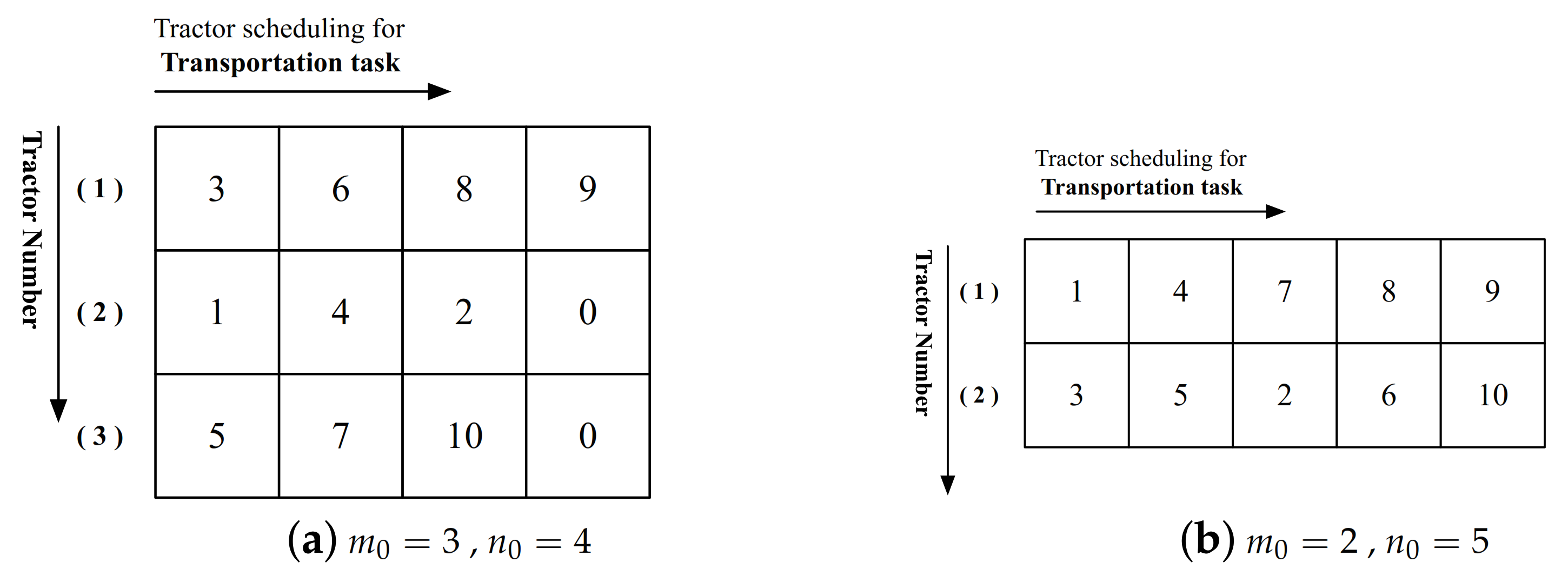
The solution can be represented as a with transportation tasks number, as shown in Figure 1. The row index means that the employed tractor number and column index shows the maximum number of transportation tasks that one tractor served. Xu et al. [52] first proposed this encoding style for self-support and 3PL vehicle scheduling problem, the row index might be the variable so-called varying dimension matrix encoding. In our study, both the row index and column index are variable and interrelated with each other. Therefore, we define our path encoding style as two-dimensional variable matrix encoding.
Special attention should be paid to tractor scheduling, which is affected by Pre-task constraint based on Equation (12), due to the above solution encoding. Consequently, we present a Infeasible-Arc filtration strategy. In each selection process of artificial ants, we extract all the optional arc and filtrate the infeasible combination. The framework of this operation is demonstrated, as shown in Algorithm 1.
| Algorithm 1: Framework of Infeasible-Arc filtration strategy. |
| INPUT: Currently solution encoding for tractors. |
| OUTPUT: Feasible-Arc Martix. |
| 1. Extract the tractor number as . |
| 2. Extract Unvisited tasks number as . |
| 3. Build a null matrices as |
| 4. for i = 1: |
| 5. for j = 1: |
| 6. if the Pre-task of task j has been visited. |
| 7. if After insert task j, tractor j had plenty of time for return trip. |
| 8. Assignment to Optional-arc Matrix . |
| 9. end |
| 10. end |
| 10. end |
| 10. end |
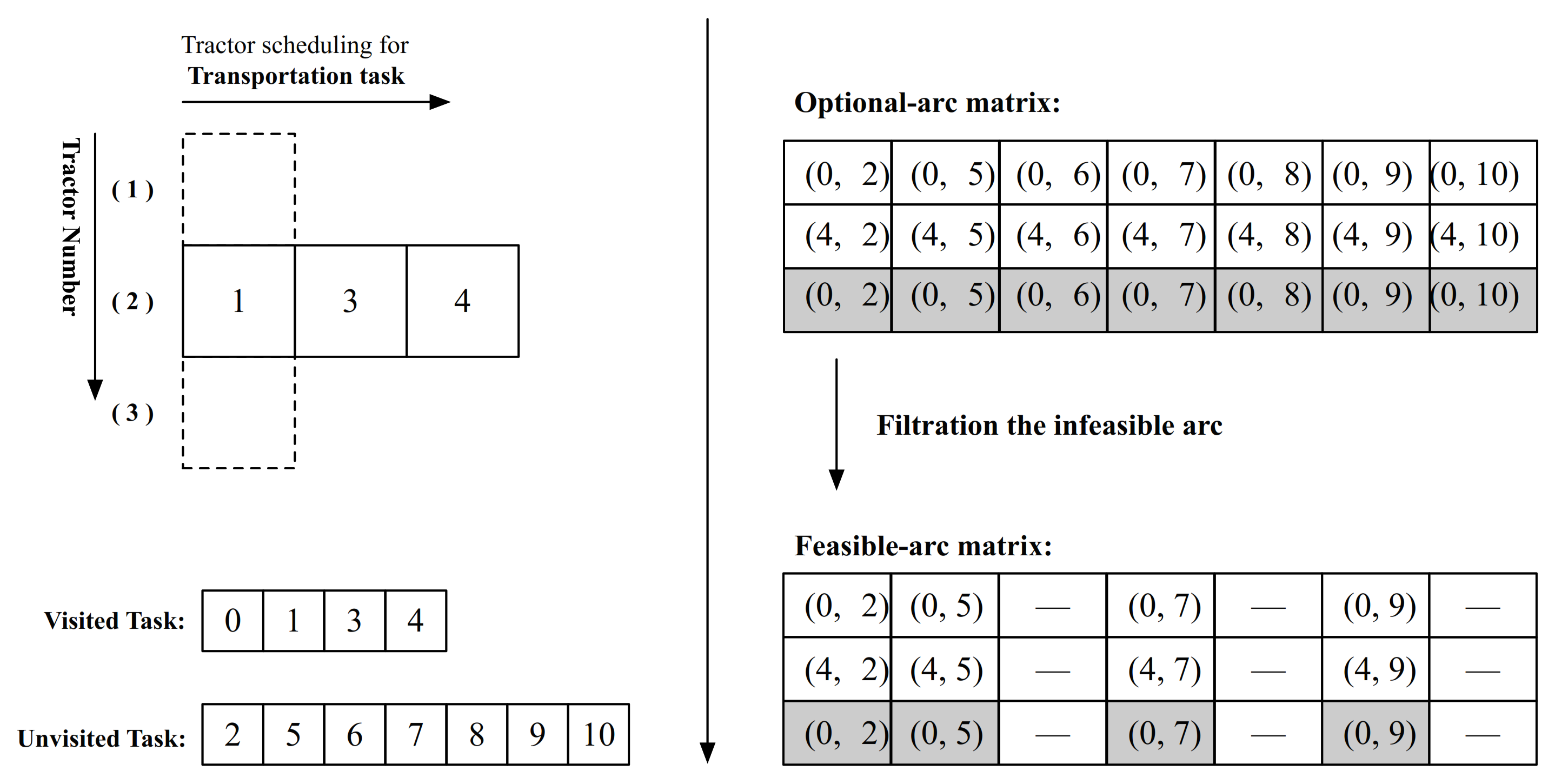
The filtration of the infeasible arc is based on the following aspect: (1) the pre-task has been selected. (2) The tractors have not broken the planning horizon in Equation (10). Figure 2 illustrates a selection process of the fourth task decision. In the initial phase, tractor 2 has three transportation tasks and parks the destination of Task 4, and tractor 1 and 3 are parked at the trailer depot. For convenience, we assume the odd-numbered tasks are the pre-task for the corresponding even-numbered tasks. The optional-arcs consist of the last task of each tractor and all of the tasks in the unvisited task set. Subsequently, we filtrate the infeasible arc and obtain the feasible-arc matrix.
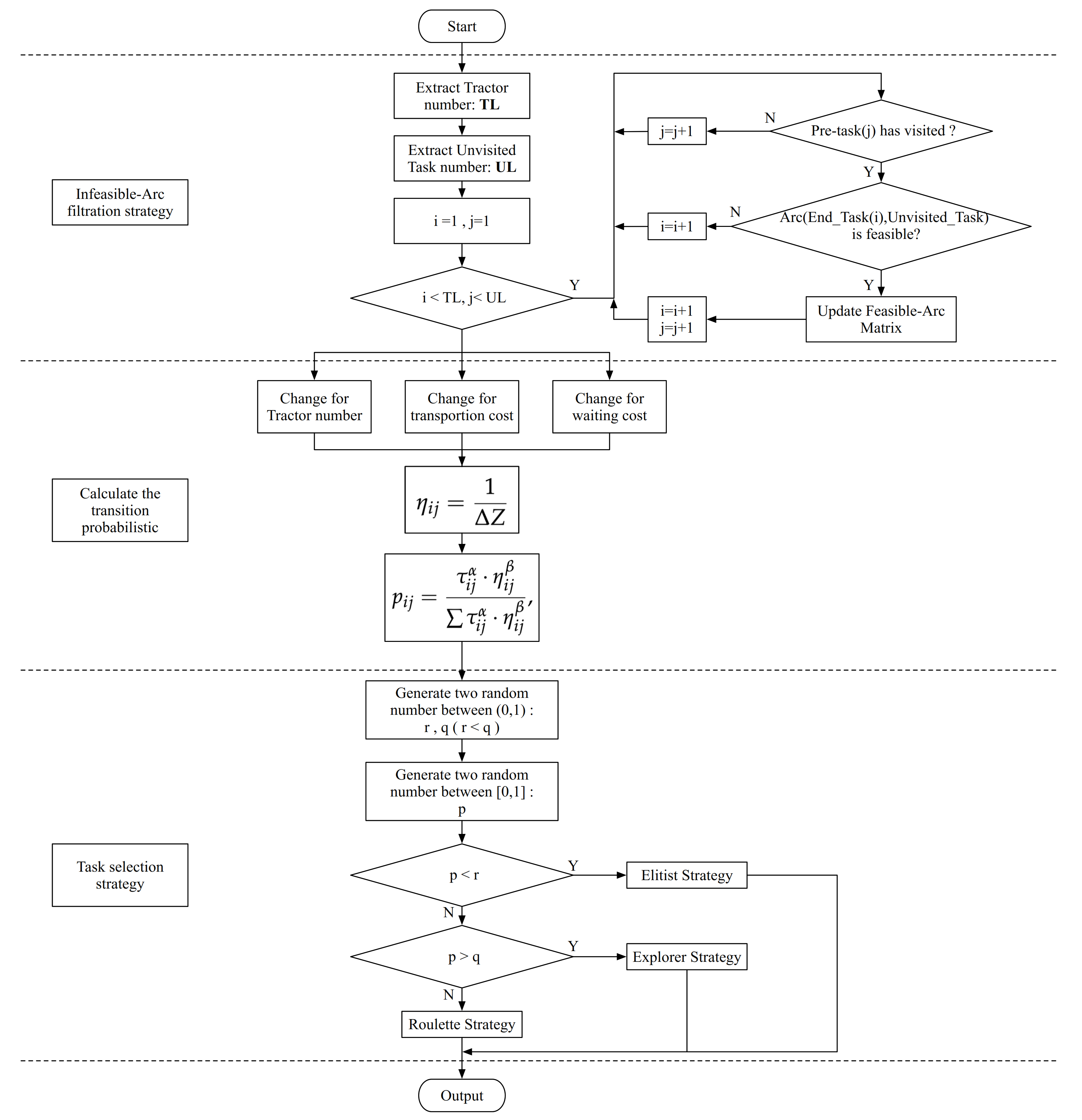
In the next step, we will calculate the transition probabilistic for each feasible-arc. First, we calculate the visibility for arc ; this parameter is affected by the objective function value, so we defined the calculation method of , as in Equation (14).
is included in the changes of the number of tractors, the connection cost for arc , and waiting time for task j. Subsequently, we could calculate the transition probabilistic , as follows:
where is pheromone level of arc , the initial value is 1, and , are two parameters that control the weight of pheromone and visibility. It is especially noted that there are a few identical elements in the Feasible-arc matrix (e.g., in Row1-Column1 and Row3-Column1), because these feasible-arcs belong to different tractors, we should calculate the transition probabilistic separately. We use three different selection strategies to improve the searching performance of ACO and prevent falling into the local best solution:
- Elitist Strategy: select the arc with a maximum transition probabilistic .
- Explorer Strategy: select one stochastic arc in a feasible-arc matrix.
- Roulette Strategy: the classical in existing ACO, where the probability for each arc corresponds to its transition probabilistic .
Figure 3 demonstrates the solution construction process.
4.2. Solution Decoding Rule and Pheromone Update Strategy
On the basis of the two-dimensional variable matrix coding system and selection strategy based on the feasible-arc matrix, as described above, a step-by-step solution decoding rule and pheromone update strategy example for Figure 1 is presented below.
- Step 1. Choose a Two-dimensional variable matrix solution.
- Step 2. Randomly select one row of this encoding. If all numbers are zero, Repeat this Step; else extract all the non-zero task number in sequence. One typical selection of tractor route in this Step is Figure 1a is “1-4-2”, for example.
- Step 3. Determine the sub-sequence of tractor route. For the example in Step 2, the sub-sequence are “0–1”, “1–4”, “4–2”, “2–0”.
- Step 4. If the objective value of this ant less than the current best solution, adopt Max–Min Ant System (MMAS) updating strategy, which only elitist ant have survived and update pheromone of sub-sequence (the pheromone update amount is , where denotes total variation for each decision step of ant and equals to objective function value of our model, and Q is pheromone update value); or else, update the whole sub-sequence pheromone of each ant.
- Step 5. Repeat Steps 2–4 until all of the tractor route in Step 1 has updated pheromone.
5. Computational Experiments
In this section, we perform numerical computational experiments to verify the performance of the proposed solution algorithm and examine the benefits of separation mode with traditional stay-with mode. The structure of this section is organized, as follows: firstly, we generate 24 small-scale and 11 large-scale test instances that are based on the benchmark of VRP with different task characteristics: Cluster, Random, and Semi-Cluster. Secondly, we present the computational results and compare them with the commercial solver. Finally, we further demonstrate the efficiency of the proposed ACO algorithm and study the scope of application. All of the procedures are embedded with ILOG Cplex optimizer (version 12.6) and Matlab R2018a 64 bit, and all of the experiments are executed on a PC with a CORE i5 CPU of 2.5 GHz and 8.0 G RAM.
5.1. Instances Generation
Our test instances are generated based on the VRP benchmark, which was first proposed by Solomon et al. [53] in accordance with presupposed rules. We determine customer number , transportation task number , inbound task number , and outbound task number , , and . Subsequently, we randomly select customer coordinate from the VRP benchmark instances, and assign one inbound task or outbound task to each customer; the remainder tasks are randomly assigned to the customers. After this step, each inbound task could be subdivided into a task and a and each outbound task could be subdivided into a task and a task. Therefore, the problem scale of generation instance is .
In addition, we assume that the tractor speeds with different vehicle states are all 40 km/h, and use Euclidean distance to conduct the transportation routes. The loading/unloading of one container is set one of the three options: 0.5 h, 1 h, 1.5 h. Referring to the calculation of fuel costs and carbon emissions costs in the literature [45], we set , , .
5.2. Small-Scale Instances
In order to demonstrate the performance metrics of the improved ACO algorithm, the optimization results are contrasted with IBM CPLEX Optimizer (version 12.6) in the same computing environment condition. We set the acceptable time constraint to 3600 s for this commercial solver, and then output the lower bound on the optimal solution and computing time (if less than 1 h). For the proposed ACO algorithm, multiple running has been simulated, and then record the best/worst/average solution and mean iteration times in Table 2.
With the increasing of transportation task number, the computation time of CPLEX has an exponential rise in atrocities and is restricted with 12 upwards scale problems, as can be seen from Table 2. This is because the interrelates and influences with pre-tasks would increase the magnitude of calculation. Moreover, the start time is another headaches in our mixed-integer programming model. However, the proposed ACO can still gain the optimal solution at an ideal time. also shows the stronger stabilizing astringency of our algorithm. For the estimation result of with different characteristic problems, the objective function values tumbled by nearly 18 percent on average. Therefore, our algorithm is able to obtain a cost-effective response to various distributed instances.
In addition, it can be seen that our approach with Random (R) distribution has comparatively better performance than the cluster (C) and semi-cluster (RC) distribution cases. On the schedule of freight process, the clustered customers tend to use traditional stay-with mode than the separation-mod. The semi-trailers and empty containers have an efficient turnover rate among these customers. However, for the Random (R) distribution cases, the tractor needs to exert much energy on their ways, the separation-mode concentrated on saving time through synchronization transportation and the loading/unloading process. Therefore, we will further demonstrate the benefit of the new operation mode through large-scale instances with Random (R) distribution.
5.3. Large-Scale Instances
This new operation is compared with the traditional stay-with mode with the improved ACO algorithm in order to demonstrate the superiority of separation mode in ICT problems. Table 3 shows the comparison result with diversity indicators. To ensure properly get the stay-with mode solutions with our algorithm, we modify the Infeasible-Arc filtration strategy of source code, which, if the Pre-task i has been visited by one tractor k, the feasible-arc of this tractor can only result in (), and . This restriction inevitably reduces the problem scale of stay-with modes. Therefore, the computation time of the stay-with mode always better than the separation mode in Table 3.
The estimation result of has shown the benefits of separation mode, which reduces the average 17.48% total transportation cost. and indicate the stability of our algorithm with different operation modes, respectively. With the enlargement of order quantity, computational complexity grows exponentially. Nevertheless, the customized improved algorithm that we designed for separation mode still maintain preferable stabilization astringency.
5.4. Performance Analysis of the Customized ACO
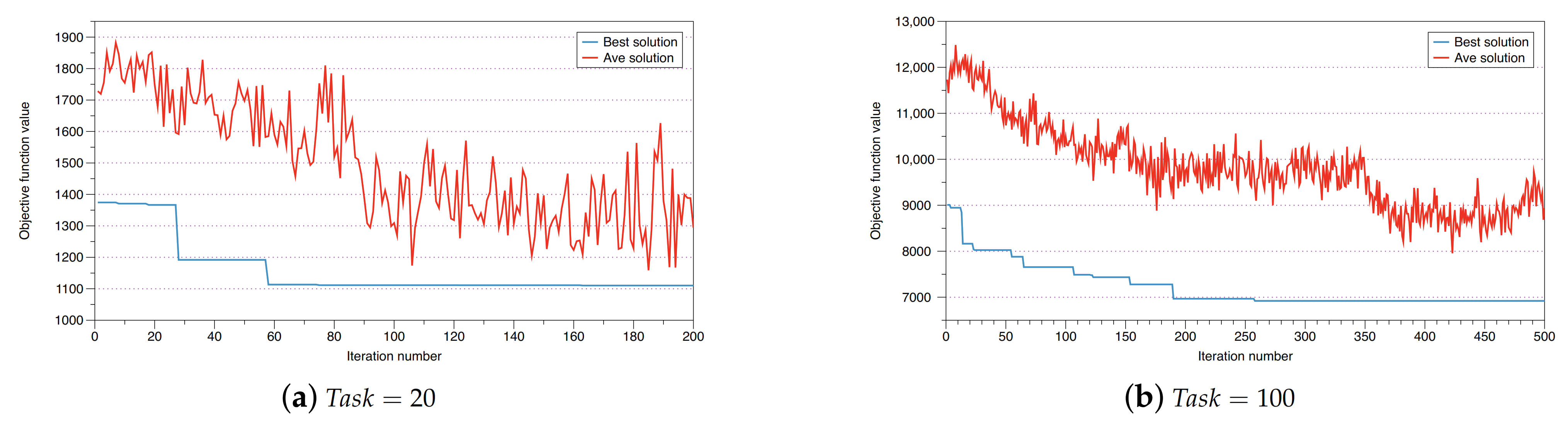
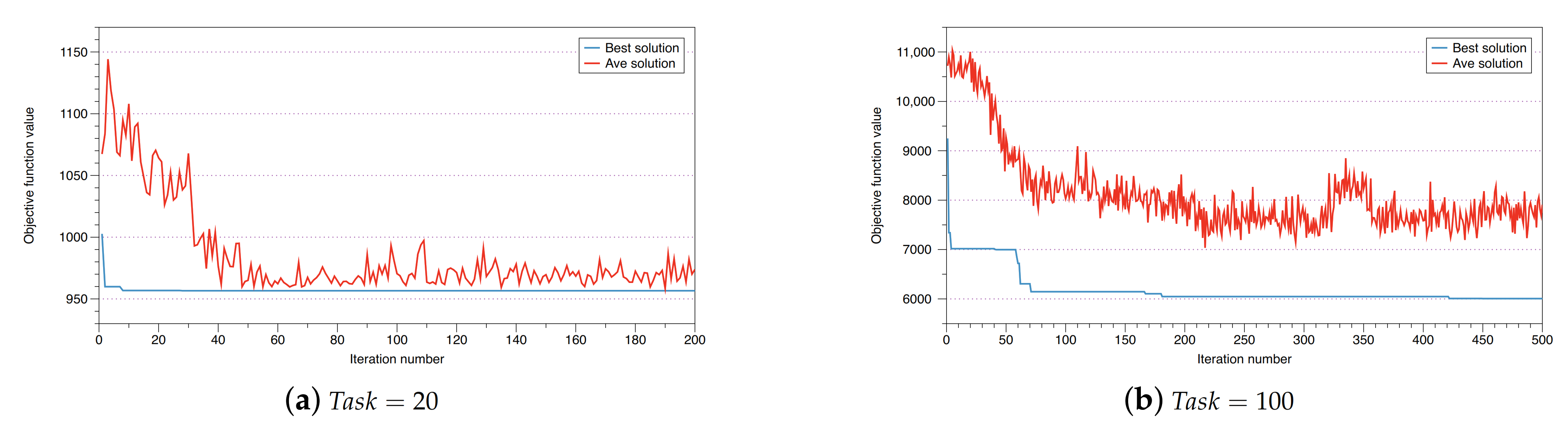
The improved ACO has comparatively better performance with Random (R) distribution, as mentioned previously. We will investigate the applicability conditions of our algorithm. Figure 4, Figure 5 and Figure 6 show the convergence of our algorithm. For the small-scale instances, the graphical representation of the results indicates excellent stability with different task characteristic distribution.
However, for the large-scale instances, the convergence speed of C and RC distribution situation are significantly less than R distribution. Especially, the algorithm searches for a new optimal solution at 465th iteration, which might indicate that the algorithm has not yet reached the steady convergence state. This is because the visibility parameter canot effectively influence the decision-making of artificial ants, in which the cluster transportation tasks have indistinguishable visibility .
6. Conclusions
The ICT problem has become an essential part of sustainable freight network construction, directly affecting fuel cost and carbon dioxide emissions. In this paper, a mixed-integer programming mathematical model with Full-Empty container integration has been proposed. Under the separation mode with tractor and semi-trailer, the pre-task constraint and carbon emission cost have been built into the model. An improved ACO algorithm with two-dimensional variable matrix encoding and Infeasible-Arc filtration strategy is designed to tackle this problem. Numerical instances with different scales and characteristics are randomly generated in order to evaluate the effectiveness of the proposed ACO algorithm. The experimental results show that our algorithm has a significant reduction in computation time and a higher overall quality of the solution.
In this study, we assume the semi-trailers and empty containers are inexhaustible. In practice, these transportation equipments are attached to different freight companies. Empty container sharing among these cooperating trucking companies is a core question, which balances the empty container flow in the freight network. Meanwhile, the multi-size trailer and container, and quantitative restrictions for trailers and empty containers will be considered in our future research work.
Author Contributions
Z.J. and S.X. proposed this research and created its framework; W.H. and Y.H. helped to collect data and analysis; S.X. completed the paper. All authors have read and approved the final manuscript.
Funding
This research is partially supported by Belt & Road Program of China Association for Science and Technology (2020ZZGJB072032), Joint Program of Liaoning Provincial Natural Science Foundation of China (2020HYLH49), Leading Talents Support Program of Dalian Municipal Government (2018-573) and Fundamental Research Funds for the Central Universities (3132019301), National Natural Science Foundation of China (71572023), European Commission Horizon 2020 (MSCA-RISE-777742-56); Leading Talents Support Program of Dalian (2018-573) and Fundamental Research Funds for the Central Universities (3132020301).
Institutional Review Board Statement
Not applicable.
Informed Consent Statement
Not applicable.
Data Availability Statement
Our research did not involve humans or animals, and did not report any data.
Conflicts of Interest
The authors declare no conflict of interest.
References
- Li, H.; Lu, Y.; Zhang, J.; Wang, T. Trends in road freight transportation carbon dioxide emissions and policies in China. Energy Policy 2013, 57, 99–106. [Google Scholar] [CrossRef]
- Demir, E.E.; Burgholzer, W.; Hrušovský, M.; Arıkan, E.; Jammernegg, W.; Van Woensel, T.T. A green intermodal service network design problem with travel time uncertainty. Transp. Res. Part B Methodol. 2016, 93, 789–807. [Google Scholar] [CrossRef]
- Shi, X.; Zhang, Y.; Voss, S. Actions applied by Chinese shipping companies under greenhouse gas emissions trading scheme. Int. J. Shipp. Transp. Logist. 2013, 5, 463–484. [Google Scholar] [CrossRef]
- Huang, Z.; Shi, X.; Wu, J.; Hu, H.; Zhao, J. Optimal annual net income of a containership using CO2 reduction measures under a marine emissions trading scheme. Transp. Lett. 2015, 7, 24–34. [Google Scholar] [CrossRef]
- Huang, Z.; Shi, X.; Wu, J.; Hu, H.; Zhao, J. How Will the Marine Emissions Trading Scheme Influence the Profit and CO2 Emissions of a Containership. In International Conference on Computational Logistics; Springer: Berlin/Heidelberg, Germany, 2013; pp. 45–57. [Google Scholar]
- Li, H. Effects of the Drop-and-Pull Transportation Mode on Mitigation of Carbon Dioxide Emissions based on the System Dynamics Model. J. Syst. 2016, 25, 514–526. [Google Scholar]
- Olivo, A.; Zuddas, P.; Di Francesco, M.; Manca, A. An operational model for empty container management. Marit. Econ. Logist. 2005, 7, 199–222. [Google Scholar] [CrossRef]
- Zhang, R.; Yun, W.Y.; Moon, I. A reactive tabu search algorithm for the multi-depot container truck transportation problem. Transp. Res. Part Logist. Transp. Rev. 2009, 45, 904–914. [Google Scholar]
- Zhang, R.; Yun, W.Y.; Kopfer, H. Heuristic-based truck scheduling for inland container transportation. OR Spectr. 2010, 32, 787–808. [Google Scholar] [CrossRef]
- Fang, L.; Xiaoning, S.; Hao, H. Analysis of Influencing Factors and Location Prediction of Dry Port Based on Logit Model. J. Chongqing Jiaotong Univ. 2012, 5, 31. [Google Scholar]
- Li, F.; Shi, X.; Hu, H. Location selection of dry port based on AP clustering-the case of southwest China. J. Syst. Manag. Sci. 2011, 1, 255–260. [Google Scholar]
- Zhang, G.; Smilowitz, K.; Erera, A. Dynamic planning for urban drayage operations. Transp. Res. Part E Logist. Transp. Rev. 2011, 47, 764–777. [Google Scholar] [CrossRef]
- Zhang, R.; Yun, W.Y.; Kopfer, H. Multi-size container transportation by truck: Modeling and optimization. Flex. Serv. Manuf. J. 2015, 27, 403–430. [Google Scholar] [CrossRef]
- Zhang, R.; Zhao, H.; Moon, I. Range-based truck-state transition modeling method for foldable container drayage services. Transp. Res. Part E Logist. Transp. Rev. 2018, 118, 225–239. [Google Scholar] [CrossRef]
- Zhang, R.; Huang, C.; Wang, J. A novel mathematical model and a large neighborhood search algorithm for container drayage operations with multi-resource constraints. Comput. Ind. Eng. 2020, 139, 106–143. [Google Scholar] [CrossRef]
- Funke, J.; Kopfer, H. A model for a multi-size inland container transportation problem. Transp. Res. Part E Logist. Transp. Rev. 2016, 89, 70–85. [Google Scholar] [CrossRef]
- van Riessen, B.; Negenborn, R.R.; Dekker, R. Real-time container transport planning with decision trees based on offline obtained optimal solutions. Decis. Support Syst. 2016, 89, 1–16. [Google Scholar] [CrossRef] [Green Version]
- Li, K.X.; Park, T.J.; Lee, P.T.W.; McLaughlin, H.; Shi, W. Container transport network for sustainable development in South Korea. Sustainability 2018, 10, 3575. [Google Scholar] [CrossRef] [Green Version]
- Fazi, S.; Roodbergen, K.J. Effects of demurrage and detention regimes on dry-port-based inland container transport. Transp. Res. Part C Emerg. Technol. 2018, 89, 1–18. [Google Scholar] [CrossRef]
- Huang, D.; Zhao, G. A Shared Container Transportation Mode in the Yangtze River. Sustainability 2019, 11, 2886. [Google Scholar]
- Shi, X.; Vanelslander, T. Design and evaluation of transportation networks: constructing transportation networks from perspectives of service integration, infrastructure investment and information system implementation. Netnomics 2010, 11, 1–4. [Google Scholar] [CrossRef] [Green Version]
- Sterzik, S.; Kopfer, H.; Yun, W.Y. Reducing hinterland transportation costs through container sharing. Flex. Serv. Manuf. J. 2015, 27, 382–402. [Google Scholar] [CrossRef]
- Song, Y.; Zhang, J.; Liang, Z.; Ye, C. An exact algorithm for the container drayage problem under a separation modes. Transp. Res. Part E Logist. Transp. Rev. 2017, 106, 231–254. [Google Scholar] [CrossRef]
- Shan, W.; Peng, Z.; Liu, J.; Yao, B.; Yu, B. An exact algorithm for inland container transportation network design. Transp. Res. Part B Methodol. 2020, 135, 41–82. [Google Scholar] [CrossRef]
- Daham, H.A.; Yang, X.; Warnes, M.K. An efficient mixed integer programming model for pairing containers in inland transportation based on the assignment of orders. J. Oper. Res. Soc. 2017, 68, 678–694. [Google Scholar] [CrossRef] [Green Version]
- Li, H.; Lv, T.; Li, Y. The tractor and semitrailer routing problem with many-to-many demand considering carbon dioxide emissions. Transp. Res. Part D Transp. Environ. 2015, 34, 68–82. [Google Scholar] [CrossRef]
- Sterzik, S.; Kopfer, H. A tabu search heuristic for the inland container transportation problem. Comput. Oper. Res. 2013, 40, 953–962. [Google Scholar] [CrossRef]
- Ji, S.; Luo, R. A hybrid estimation of distribution algorithm for multi-objective multi-sourcing intermodal transportation network design problem considering carbon emissions. Sustainability 2017, 9, 1133. [Google Scholar]
- Vidović, M.; Popović, D.; Ratković, B.; Radivojevic, G. Generalized mixed integer and VNS heuristic approach to solving the multisize containers drayage problem. Int. Trans. Oper. Res. 2017, 24, 583–614. [Google Scholar] [CrossRef]
- Chao, I.M. A tabu search method for the truck and trailer routing problem. Comput. Oper. Res. 2002, 29, 33–51. [Google Scholar] [CrossRef]
- Tan, K.C.; Chew, Y.H.; Lee, L.H. A hybrid multi-objective evolutionary algorithm for solving truck and trailer vehicle routing problems. Eur. J. Oper. Res. 2006, 172, 855–885. [Google Scholar] [CrossRef]
- Lin, S.W.; Vincent, F.Y.; Chou, S.Y. Solving the truck and trailer routing problem based on a simulated annealing heuristic. Comput. Oper. Res. 2009, 36, 1683–1692. [Google Scholar] [CrossRef]
- Villegas, J.G.; Prins, C.; Prodhon, C.; Medaglia, A.L.; Velasco, N. A GRASP with evolutionary path relinking for the truck and trailer routing problem. Comput. Oper. Res. 2011, 38, 1319–1334. [Google Scholar] [CrossRef]
- Villegas, J.G.; Prins, C.; Prodhon, C.; Medaglia, A.L.; Velasco, N. A matheuristic for the truck and trailer routing problem. Eur. J. Oper. Res. 2013, 230, 231–244. [Google Scholar] [CrossRef]
- Lu, Y.; Lang, M.; Yu, X.; Li, S. A Sustainable Multimodal Transport System: The Two-Echelon Location-Routing Problem with Consolidation in the Euro—China Expressway. Sustainability 2019, 11, 5486. [Google Scholar] [CrossRef] [Green Version]
- Yang, Z.H.; Yang, G.M.; Xu, Q.; Guo, S.J.; Jin, Z.H. Optimization on tractor-and-trailer transportation scheduling with uncertain empty-trailer tasks. J. Traffic Transp. Eng. 2016, 16, 103–111. [Google Scholar]
- Xue, Z.; Lin, W.-H.; Miao, L.; Zhang, C. Local container drayage problem with tractor and trailer operating in separable mode. Flex. Serv. Manuf. J. 2015, 27, 431–450. [Google Scholar] [CrossRef]
- Xue, Z.; Zhang, C.; Lin, W.-H.; Miao, L.; Yang, P. A tabu search heuristic for the local container drayage problem under a new operation mode. Transp. Res. Part E Logist. Transp. Rev. 2014, 62, 136–150. [Google Scholar] [CrossRef]
- Caballini, C.; Sacone, S.; Saeednia, M. Cooperation among truck carriers in seaport containerized transportation. Transp. Res. Part E Logist. Transp. Rev. 2016, 93, 38–56. [Google Scholar] [CrossRef]
- Sun, Q.; Sun, J.; Jin, Z.; Sun, S. Mode selection of tractor-and-semitrailer swap transport for ro-ro shipping under land-sea combined transportation. Marit. Policy Manag. 2019, 46, 995–1010. [Google Scholar] [CrossRef]
- Liao, C.-H.; Tseng, P.-H.; Cullinane, K.; Lu, C.-S. The impact of an emerging port on the carbon dioxide emissions of inland container transport: An empirical study of Taipei port. Energy Policy 2010, 38, 5251–5257. [Google Scholar] [CrossRef]
- Jaehun, S. A carbon emission evaluation model for a container terminal. J. Clean. Prod. 2018, 186, 526–533. [Google Scholar]
- Hung, G.S. The impact of foldable ocean containers on back haul shippers and carbon emissions. Transp. Res. Part D Transp. Environ. 2019, 67, 514–527. [Google Scholar]
- Hoen, K.M.R.; Tan, T.; Fransoo, J.C.; Van Houtum, G.J. Effect of carbon emission regulations on transport mode selection under stochastic demand. Flex. Serv. Manuf. J. 2014, 26, 170–195. [Google Scholar] [CrossRef] [Green Version]
- Fan, H.; Ren, X.; Guo, Z.; Li, Y. Truck Scheduling Problem Considering Carbon Emissions under Truck Appointment System. Sustainability 2019, 11, 6256. [Google Scholar] [CrossRef] [Green Version]
- Li, L.; Zhang, X. Integrated optimization of railway freight operation planning and pricing based on carbon emission reduction policies. J. Clean. Prod. 2020, 263, 121316. [Google Scholar] [CrossRef]
- Yin, C.; Ke, Y.; Yan, Y.; Lu, Y.; Xu, X. Operation Plan of China Railway Express at Inland Railway Container Center Station. Int. J. Transp. Sci. Technol. 2020, 9, 249–262. [Google Scholar] [CrossRef]
- Thai, P.H.; Lee, H. Developing a green route model for dry port selection in Vietnam. Asian J. Shipp. Logist. 2019, 35, 96–107. [Google Scholar]
- Tsao, Y.-C.; Linh, V.T. Seaport-dry port network design considering multimodal transport and carbon emissions. J. Clean. Prod. 2018, 199, 481–492. [Google Scholar] [CrossRef]
- Qiu, X.; Lam, J.S.L. The value of sharing inland transportation services in a dry port system. Transp. Sci. 2018, 52, 835–849. [Google Scholar] [CrossRef]
- Yuvraj, G.; Abad, P. An ant colony system (ACS) for vehicle routing problem with simultaneous delivery and pickup. Comput. Oper. Res. 2009, 36, 3215–3223. [Google Scholar]
- Xu, S.; Liu, Y.; Chen, M. Optimisation of partial collaborative transportation scheduling in supply chain management with 3PL using ACO. Expert Syst. Appl. 2017, 71, 173–191. [Google Scholar] [CrossRef]
- Solomon, M.M. Algorithms for the vehicle routing and scheduling problems with time window constraints. Oper. Res. 1987, 35, 254–265. [Google Scholar] [CrossRef] [Green Version]
Figure 1.
Two typical solution encoding of 10 tasks with different number of tractors.

Figure 2.
The generation of the feasible-arc matrix.

Figure 3.
Demonstration of solution construction process.

Figure 4.
Convergence of customized ant colony optimization (ACO) with Cluster distribution.

Figure 5.
Convergence of customized ACO with Random distribution.

Figure 6.
Convergence of customized ACO with Semi-cluster distribution.


Table 1.
The Tractor operation of Link-arc with different classification tasks.
| - | Drive to full container yard | Drive to the Receiver location | Drive to empty container yard Pickup empty container Drive to the Shipper location | Drive to the Shipper location | |
| Back to trailer depot | Drive to the trailer depot Pull on a trailer Drive to full container yard | Drive to the Receiver location | Drive to the trailer depot Pull on a trailer Drive to empty container yard Pickup empty container Drive to the Shipper location | Drive to the Shipper location | |
| Drive to empty container yard Drop the empty container solely Back to trailer depot | Drive to empty container yard Drop the empty container solely Drive to full container yard | Drive to empty container yard Drop the empty container solely Drive to the trailer depot Drop off a trailer Drive to the Receiver location | Drive to the Shipper location | Drive to empty container yard Drop the empty container solely Drive to the trailer depot Drop off a trailer Drive to the Shipper location | |
| Back to trailer depot | Drive to the trailer depot Pull on a trailer Drive to full container yard | Drive to the Receiver location | Drive to the trailer depot Pull on a trailer Drive to empty container yard Pickup empty container Drive to the Shipper location | Drive to the Shipper location | |
| Back to trailer depot | Stay at heavy container yard | Drive to the trailer depot Drop off a trailer Drive to the Receiver location | Drive to empty container yard Pickup empty container Drive to the Shipper location | Drive to the trailer depot Drop off a trailer Drive to the Shipper location |
Table 2.
Performance comparison for small-scale instances with various distributions.
| Dst. | Scale | Task | Commercial Solver | Improved ACO | (%) | (%) | ||||
|---|---|---|---|---|---|---|---|---|---|---|
| CPU | CPU | |||||||||
| C | 4-C | 1/1/1/1 | 332.721 | 0.17 | 332.721 | 332.721 | 332.721 | 0.52 | 0 | 0 |
| 6-C | 1/1/2/2 | 331.183 | 0.34 | 331.183 | 331.183 | 331.183 | 0.73 | 0 | 0 | |
| 6-C | 2/2/1/1 | 331.265 | 0.40 | 331.265 | 331.265 | 331.265 | 0.78 | 0 | 0 | |
| 8-C | 1/1/3/3 | 354.255 | 6.99 | 354.255 | 354.255 | 354.255 | 1.50 | 0 | 0 | |
| 8-C | 2/2/2/2 | 351.938 | 9.51 | 351.938 | 351.938 | 351.938 | 1.53 | 0 | 0 | |
| 10-C | 2/2/3/3 | 452.071 | 421.67 | 452.071 | 454.403 | 453.006 | 2.08 | 0 | 0.21 | |
| 12-C | 3/3/3/3 | 830.999 | 3600 | 746.601 | 789.913 | 776.838 | 5.31 | 10.16 | 4.05 | |
| 16-C | 4/4/4/4 | 1032.308 | 3600 | 780.542 | 846.301 | 811.051 | 5.66 | 24.39 | 3.91 | |
| R | 4-R | 1/1/1/1 | 342.529 | 0.40 | 342.529 | 342.529 | 342.529 | 0.55 | 0.00 | 0.00 |
| 6-R | 1/1/2/2 | 300.000 | 0.52 | 300.000 | 300.000 | 300.000 | 0.84 | 0.00 | 0.00 | |
| 6-R | 2/2/1/1 | 309.252 | 0.63 | 309.252 | 309.252 | 309.252 | 0.85 | 0.00 | 0.00 | |
| 8-R | 1/1/3/3 | 316.540 | 7.36 | 316.540 | 316.540 | 316.540 | 1.05 | 0.00 | 0.00 | |
| 8-R | 2/2/2/2 | 331.790 | 12.34 | 331.790 | 331.790 | 331.790 | 1.26 | 0.00 | 0.00 | |
| 10-R | 2/2/3/3 | 453.292 | 661.11 | 453.292 | 503.865 | 495.169 | 2.76 | 0.00 | 9.24 | |
| 12-R | 3/3/3/3 | 774.703 | 3600 | 686.196 | 732.741 | 719.969 | 4.89 | 11.42 | 4.92 | |
| 16-R | 4/4/4/4 | 1154.970 | 3600 | 765.292 | 823.932 | 804.578 | 7.40 | 33.74 | 5.13 | |
| RC | 4-RC | 1/1/1/1 | 322.275 | 0.31 | 322.275 | 322.275 | 322.275 | 0.59 | 0.00 | 0.00 |
| 6-RC | 1/1/2/2 | 360.371 | 0.55 | 360.371 | 360.371 | 360.371 | 0.84 | 0.00 | 0.00 | |
| 6-RC | 2/2/1/1 | 357.678 | 0.41 | 357.678 | 357.678 | 357.678 | 0.93 | 0.00 | 0.00 | |
| 8-RC | 1/1/3/3 | 355.796 | 9.45 | 355.796 | 355.796 | 355.796 | 1.09 | 0.00 | 0.00 | |
| 8-RC | 2/2/2/2 | 397.043 | 6.55 | 397.043 | 397.043 | 397.043 | 1.26 | 0.00 | 0.00 | |
| 10-RC | 2/2/3/3 | 821.319 | 242.93 | 723.373 | 776.307 | 766.909 | 1.41 | 11.93 | 6.02 | |
| 12-RC | 3/3/3/3 | 854.553 | 3600 | 717.856 | 803.346 | 766.660 | 5.27 | 16.00 | 6.80 | |
| 16-RC | 4/4/4/4 | 979.120 | 3600 | 752.427 | 835.855 | 790.760 | 8.60 | 23.15 | 5.09 | |
| Average | 18.68 | 5.13 | ||||||||
Scale: n-X stand for the n transportation tasks with X characteristic distribution. ; Task: m/n/k/l stand for the task number of , , , , respectively. : the lower bound on the optimal solution; CPU: Computation time for CPLEX and proposed ACO; Gap1 = (LB − Opt)/LB; Gap2 = (Ave − Opt)/Opt.
Table 3.
Performance comparison for large-scale instances with Random (R) distributions.
| No. | Scale | Stay-With Mode | Separation Mode | (%) | (%) | (%) | ||||
|---|---|---|---|---|---|---|---|---|---|---|
| CPU | CPU | |||||||||
| 1 | 20-R | 1129.815 | 1143.228 | 10.19 | 940.749 | 947.871 | 11.55 | 16.73 | −1.19 | −0.757 |
| 2 | 30-R | 1205.287 | 1256.424 | 12.50 | 1110.288 | 1151.889 | 32.67 | 7.88 | −4.24 | −3.747 |
| 3 | 30-R | 1718.442 | 1794.912 | 20.64 | 1372.741 | 1427.110 | 27.58 | 20.12 | −4.45 | −3.961 |
| 4 | 30-R | 1721.429 | 1805.311 | 21.42 | 1414.490 | 1469.680 | 32.19 | 17.83 | −4.87 | −3.902 |
| 5 | 40-R | 2300.307 | 2469.760 | 103.43 | 1955.706 | 2062.820 | 136.39 | 14.98 | −7.37 | −5.477 |
| 6 | 60-R | 3512.034 | 4106.269 | 426.39 | 3038.304 | 3277.800 | 524.04 | 13.49 | −16.92 | −7.883 |
| 7 | 80-R | 4994.781 | 6006.973 | 662.64 | 4241.813 | 4850.220 | 923.31 | 15.08 | −20.26 | −14.343 |
| 8 | 100-R | 6526.592 | 8207.964 | 1178.31 | 5458.694 | 6293.559 | 2091.55 | 16.36 | −25.76 | −15.294 |
| 9 | 120-R | 8843.383 | 10,717.706 | 2222.92 | 6920.267 | 8411.912 | 3170.94 | 21.75 | −21.19 | −21.555 |
| 10 | 160-R | 11,324.120 | 15,363.589 | 4609.23 | 9016.639 | 11,991.371 | 7939.20 | 20.38 | −35.67 | −32.992 |
| 11 | 200-R | 16,598.903 | 23,704.445 | 10,346.77 | 11,994.986 | 18,404.399 | 14,680.57 | 27.74 | −42.81 | −53.434 |
| Ave | 17.48 | −16.79 | −14.85 | |||||||
Scale: n-X stand for the n transportation tasks with X characteristic distribution. ; Task: m/n/k/l stand for the task number of , , , , respectively. Gap1 = (Opta − Optb)/Opta; Gap2 = (Opta − Avea)/Opta; Gap3 = (Optb − Aveb)/Optb.
Publisher’s Note: MDPI stays neutral with regard to jurisdictional claims in published maps and institutional affiliations. |
© 2021 by the authors. Licensee MDPI, Basel, Switzerland. This article is an open access article distributed under the terms and conditions of the Creative Commons Attribution (CC BY) license (http://creativecommons.org/licenses/by/4.0/).
Share and Cite
MDPI and ACS Style
He, W.; Jin, Z.; Huang, Y.; Xu, S. The Inland Container Transportation Problem with Separation Mode Considering Carbon Dioxide Emissions. Sustainability 2021, 13, 1573. https://0-doi-org.brum.beds.ac.uk/10.3390/su13031573
AMA Style
He W, Jin Z, Huang Y, Xu S. The Inland Container Transportation Problem with Separation Mode Considering Carbon Dioxide Emissions. Sustainability. 2021; 13(3):1573. https://0-doi-org.brum.beds.ac.uk/10.3390/su13031573
Chicago/Turabian StyleHe, Wenqing, Zhihong Jin, Ying Huang, and Shida Xu. 2021. "The Inland Container Transportation Problem with Separation Mode Considering Carbon Dioxide Emissions" Sustainability 13, no. 3: 1573. https://0-doi-org.brum.beds.ac.uk/10.3390/su13031573
Note that from the first issue of 2016, this journal uses article numbers instead of page numbers. See further details here.