Article

Large-Area Empirically Based Visual Landscape Quality Assessment for Spatial Planning—A Validation Approach by Method Triangulation

1
Landscape Planning, Especially Landscape Informatics, School of Environment/Design/Therapy, Nürtingen-Geislingen University, 72622 Nürtingen, Germany
2
Institute of Landscape and Environment, Nürtingen-Geislingen University, 72622 Nürtingen, Germany
3
Landscape Ecology and Geographical Information Systems, Faculty of Agriculture/Environment/Chemistry, Dresden University of Applied Sciences, 01069 Dresden, Germany
4
Leibniz Institute of Ecological Urban and Regional Development, Research Area Landscape Change and Management, 01217 Dresden, Germany
*
Author to whom correspondence should be addressed.
Sustainability 2021, 13(4), 1891; https://0-doi-org.brum.beds.ac.uk/10.3390/su13041891
Submission received: 25 January 2021 / Revised: 5 February 2021 / Accepted: 6 February 2021 / Published: 9 February 2021
(This article belongs to the Special Issue Visual Landscape Research in Sustainable Urban and Landscape Planning)

Abstract

:
Large area visual landscape quality assessment, especially at the national level is needed to answer the demand from strategic planning. In our paper, we describe and compare two recent modelling approaches for this task regarding their theoretical and empirical basis, resolution, model configuration and results. To compare the outcomes of the two methods, both correlation measures and a visual overlay analysing the inversions are used. The results show, that despite the different methodological approaches, in over 90% of the area of Germany there are only minor deviations between the resulting scenic quality maps (less or equal one step on a five-step scale). The main differences occur due to a different relative weight given to terrain and water indicators in the respective methods. We conclude that a methodologically valid scenic quality evaluation using geodata of homogenous quality is possible also at the national level. By triangulating between different methods, for both, the validity could be proven. The datasets elaborated can also be used as a benchmark for regional landscape assessments and for an upcoming monitoring of changes in visual landscape quality.

1. Introduction

At the outset, we would like to formulate our guiding question: “What is a large-area assessment of landscape scenery needed for?” In seeking an answer, we here propose the thesis that planning information on the quality of landscape scenery is essential at the national level. And certainly, we can confirm that spatial planning—not just in Germany but worldwide—is increasingly being carried out by national authorities. It is clear that development and implementation tasks are ever more frequently assigned to the national level in order to ensure a more coordinated and harmonized spatial development. Growing disparities between regions can only be overcome by means of supra-regional models and spatial plans. In addition, EU guidelines frequently demand that planning take place at national level, at least within the European Union, for example through directives to establish a Natura 2000 network of nature reserves [1] or measures to develop national concepts for ‘green infrastructure’ in Member States [2]. In Germany, the implementation of the requirement to establish a Europe-wide Natura 2000 network is the responsibility of the individual Länder (i.e., German federal states). Yet past experience has shown that success can only be achieved through the close cooperation of the various Länder with a specific focus on the national context. This applies, for example, to coordinated management planning for Natura 2000 sites. In order to achieve a favourable conservation status for a habitat type or species, it is precisely the overarching goals at the biogeographical and thus possibly federal states transboundary or even national level that must be taken into account (cf. [3] p. 306). In this case, only a broader and cooperative perspective of management planning leads to overall success. Recently, Germany has also adopted a national concept for ‘green infrastructure’, whereby important natural features and areas are brought together in a strategic network covering all the Länder. The aim in drawing up this network is to aid spatial planning [4] by providing information on ecosystem services. This can assist, for example, in federal planning for transport infrastructure [5] or to expand Germany’s electricity grid by minimizing or compensating impacts on ecosystem services and green infrastructure. Strategic Environmental Assessments of federal plans and programmes are important instruments that require precisely such highly aggregated, nationwide information on the environment and landscapes [6]. In this respect, it is only logical that, in addition to physical-material data on ecosystem services at federal level, large-scale information on cultural ecosystem services is now also being prepared, especially on landscape scenery qualities. This has become necessary to cope with the expansion of the federal electricity grid within the country’s ambitious Energiewende (i.e., the transition to an energy system based on renewable energy) as well as the processes of public participation that it entails.
The horizontal, cross-sectoral need at federal level for data on the environment, nature conservation and landscapes is accompanied vertically by demands at the level of Germany’s Länder and regions. It is becoming increasingly clear that nationwide standardized data on landscapes are also required at the regional planning level [7] or even local level [8]; for example, in order to better compare the development of tourism or recreation-related qualities in different areas (with their specific landscape conditions) for regional or landscape planning. This can help establish a benchmark for tourist regions. Information on landscape scenery qualities at federal level is thus also demanded in Germany by planning levels lower down the vertical hierarchy.
High-resolution data and information is now also on hand to help deal with complex tasks of spatial coordination at federal level for the purposes of spatial development (see, for example, the IOER Monitor of Settlement and Open Space Development [9]). Such sources of data mean that planning at federal level is not limited to purely theoretical considerations but can also be presented at this planning level in great detail with corresponding GIS zoom functions across a range of scales. Thus, technological progress in data gathering and presentation also aids the development of concrete planning goals at federal level. Summarizing, we can say that a large-scale assessment of landscapes and landscape scenery is needed by the national authorities in Germany to secure an empirical basis for a wide variety of new tasks. This need of data on the visual landscape as an input to spatial planning is also confirmed for other countries and planning levels such as coastal landscapes in the French Mediterranean [10], visual impacts caused by wind turbines in parts of Austria, Germany, Poland and the Czech Republic [11], or planning and decision support systems in Switzerland [12].
Looking at both landscape quality assessments and landscape planning in practice in Germany, it can be observed, that methodologically sound visual landscape quality assessment models with an empirical basis, using geodata of homogenous quality, and covering whole federal states or even the whole of Germany were either not existent or were not used in the past [13,14]. Thus, the aim of this paper is to present and compare two modelling approaches addressing visual landscape quality at the national level, and to compare their results in order to cross-validate the underlying methodologies by a method triangulation approach.

2. Materials and Methods

In this paper, we compare two approaches for nationwide visual landscape quality assessment. Walz & Stein developed the first in 2016 [15] using spatial data, providing a nationwide standardised evaluation to be used for the “regular monitoring to make changes over time visible” [15] (p. 65). Roth et al. [16] invented the second method, which in addition to nationwide standardized geodata used a large survey on landscape perception and empirical landscape quality assessment as a basis to statistically model perceived landscape quality. Both methods are based on human perception of landscapes, be it indirect through the selection of parameters that have “a relation to the perception of landscape by humans” [15] (p. 65) or direct through a representative survey on landscape perception [16]. Thus, both approaches are in line with the landscape definition of the European Convention [17] that defines landscape as “an area, as perceived by people, whose character is the result of the action and interaction of natural and/or human factors.” In the following sections, we describe the methodological approaches including the underlying theories, the data used and the results of the two respective methods, before we compare their results and draw some conclusions.

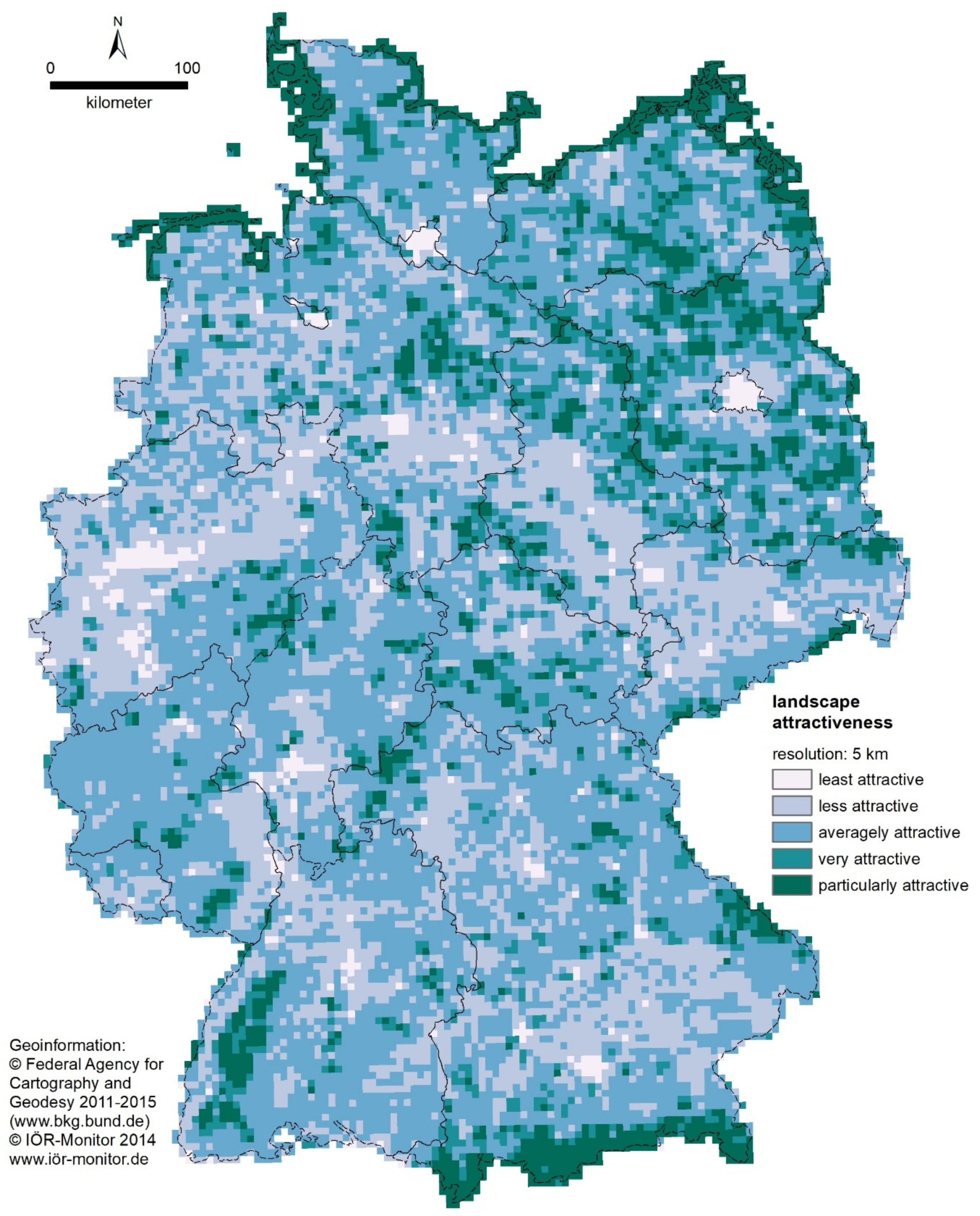
2.1. Landscape Attractiveness (Method Walz & Stein)

2.1.1. Underlying Theory

In the method used by Walz & Stein, the attractiveness of the landscape is derived from the natural features of the landscape and the way it is shaped by man. This model, which basically represents a suitability analysis of a region for nature-related recreation, is based on the assumption that certain features of the landscape have a positive or negative effect on the attractiveness of the landscape and its suitability for recreation.
The basic idea is to carry out a comparable landscape assessment for the whole of Germany on the basis of existing geodata. This will enable regular repetition in the future. Local surveys or questionnaires are therefore out of the question. Instead, parameters or sub-indicators are used which have been cited in the literature as relevant and some of which have been checked for plausibility by means of surveys. These include the methods according to Kiemstedt [18]; Briggs & France [19]; Marks [20]; Chen et al. [21]; Augenstein [22]; Berger & Walz [23]; Federal Office for Building and Regional Planning (BBR) [24] and Roth & Gruehn [25,26]. More recent publications that also use existing geodata to determine the attractiveness of landscapes include Frank et al. [27]; Schirpke et al. [28]; Schüpbach et al. [29] and Hermes et al. [30]. Roth & Bruns [31] provide an overview of the topic for the German-speaking countries.

2.1.2. Description of the Approach and Evaluation Method (including Justification of the Choice of Indicators)

The method used here was initially developed for a nationwide study to analyse possible effects of landscape planning in spatial terms [32]. Following Berger & Walz [23], Chen et al. [21] and BBR [24] (p. 209), positive value-giving parameters such as the diversity of relief, the proportion of open space, the hemeroby index, the wood-dominated ecotone density, the density of watercourse edges, the coastlines and the proportion of unfragmented open spaces > 50 km2 were used. This is based on the assumption that people feel most at home in a landscape that is diverse and varied, with a high proportion of near-natural areas, and that these are therefore particularly attractive for recreational purposes [33].
In a further step, this methodology was supplemented by landscape elements of the technical infrastructure, which negatively influence the suitability of the landscape for the mentioned purposes (see also contributions in [34]). Specifically, these are high-voltage power lines, wind turbines and solar fields. The supplemented methodology was published in Walz & Stein [15].
The parameters are in detail:
The topographic diversity (ratio 3D/2D) [35] reflects not only the maximum height difference (relief energy) but also the cumulative height differences. Relief contributes significantly to the diversity of a landscape and the resulting variety perceived by man [36]. A high value promises a good overview of the landscape, provides views and makes the landscape more interesting. According to Augenstein [22], views have a positive effect in so far as they stimulate the exploration and interpretation of the landscape through the newly emerging visual relationships.
The proportion of undeveloped areas is indicated by the open space percentage. We followed the definition of open space in a landscape ecological and landscape architectureal understanding [37] as the opposite of built-up space. Thus, open space is the part of the landscape that is not covered by buildings or traffic infrastructure. A low proportion of open space indicates urban or densely built-up village areas, which can weaken the natural attractiveness of the landscape due to the strong overshadowing by technical artefacts. A higher proportion of open space also increases the perceived closeness to nature [22] and thus the attractiveness. This includes forests, grassland areas, but also arable land. Nohl [38] notes that grassland landscapes in Germany have traditionally been important for tourism because they are perceived as aesthetic and attractive landscapes.
The hemeroby index is a surface-weighted average of the hemeroby levels of all land uses. The hemeroby index as a measure of human influence gives the open space component a weighting in terms of naturalness and land use. Naturalness is an important factor for the attractiveness of landscapes [22,39,40]. Data from Walz & Stein [41] based on the LBM-DE 2009 and the potential natural vegetation of Germany were used.
The density of ecotones dominated by woody plants takes into account the diversity and structure of the landscape. This parameter characterises above all variety and edge effects. In ecology, an ecotone is defined as a transition zone between two different ecosystems. Woody and forest edges, tree rows and hedges play an important role in this context. The more such elements are present in a landscape, the more structured it is. A variety of studies and procedures for landscape perception and assessment [20,42] assume that landscape diversity, which is significantly influenced by marginal effects such as ecotones, increases the recreational and experience value. This parameter consists of lines representing woody and forest edges, as well as rows of trees and hedges. The density (km/km2) of the ecotones for the reference area is determined for this parameter. The less straightened the course of these lines is and the more lines there are, the higher is the density of the linear elements. A high density promises a pronounced complexity, which gives the impression of undisturbed area expansion and thus closeness to nature [36].
Another measure of landscape diversity and structure is the ratio of riparian areas. Watercourses have a considerable influence on the landscape and thus on its attractiveness [18,20]]. Transitional areas between water (blue) and vegetation (green) are particularly attractive. In the case of lakes, the length of the banks is decisive for those seeking recreation (cf. [43]). By taking watercourse edges into account, smaller lakes and, above all, running waters also attract attention. This parameter reflects the density (km/km2) of all water bodies, except for artificial waterways such as canals and temporary water bodies.
As the coasts play a very important role in terms of attractiveness and recreation [40], they are represented by the independent parameter coastlines. The values of this parameter are entered into the indicator with “1” (raster cell has a share of coast) or with “0” (raster cell has no share of coast).
With the proportion of unfragmented open spaces larger than 50 km2, the undisturbedness of landscape areas by the fragmenting supra-local transport network is included as a value-giving factor. Coherent forests, woodlands, heaths and other ecologically valuable areas are of great importance as habitats for animals and plants and as recreational areas for humans [44]. The large areas, which in the selection of the dataset only cover those not fragmented by traffic corridors with high traffic volume and bigger than 50 km2 are quiet and contain no barriers due to traffic routes. High proportions occur in sparsely populated regions with low traffic density. In addition to ecologically valuable areas, however, numerous large unfragmented areas also show intensive use (e.g., agriculture or open-cast mines) [44].
The technical infrastructure for the production and transport of renewable energies was taken into account by including the number of wind turbines, the proportion of solar fields and the length of high-voltage lines (see also [45]).

2.1.3. Data Used

In accordance with the above-mentioned objective of the method to provide nationwide comparable results that can be repeated regularly, only data sources that are collected nationwide using comparable methods and updated regularly were considered. Only data from the official surveying authorities fulfil these requirements. In this context, simplifications had to be accepted due to the content and spatial resolution of the geodata regularly collected nationwide.
All parameters used were collected on the basis of the Official Topographic-Cartographic Information System (ATKIS Basis-DLM) or the land cover model (LBM-DE), both dating from 2010, which were the most up-to-date nationwide datasets available at the time of the original project. These are officially collected land use data in vector format by the State and Federal Surveying Authorities. The values of the parameters relief diversity, proportion of open space, hemeroby and ecotone density, wind turbine density and proportion of photovoltaic open space systems are freely available in the IÖR-Monitor (www.ioer-monitor.de; accessed on 8 February 2021).

2.1.4. Resolution, Raster Width of the Grid

The indicator of landscape attractiveness presented here was calculated on the basis of a 5 km grid (according to INSPIRE). The use of the INSPIRE grid was important in order to remain connectable to the European monitoring systems. The INSPIRE spatial units will in future be the applicable reference units for monitoring in various disciplines in Germany. In order to transfer the result values to municipalities (see map in [15]), the average value of all grid cells touched was then given for the municipal areas. This prevents small-scale effects from having too strong impacts on the attractiveness value. The influence of different sizes of municipalities is also mitigated. The inclusion of all grid cells that intersect the municipality also takes into account the fact that the attractiveness of the landscape does not change abruptly at municipal boundaries and that there are visual relationships with the surrounding landscape.

2.1.5. Equal Weighting of All Indicators

All parameters were standardised between 0 and 1 and then summed up. This ensures that all parameters are equally weighted in the total value. No weighting was deliberately applied, as Kiemstedt [18], for example, suggested when calculating the experience value of a landscape (v-value). This lacks an objective basis for evaluation, which would make the methodology less comprehensible.

2.1.6. Correlation of the Parameters with Each Other

It was also crucial for the choice of parameters that they did not correlate with each other. This can be ruled out except for a moderate correlation between the hemeroby index and relief diversity (r = −0.403; N = 14,589) and the proportion of open space and hemeroby (r = −0.491; N = 14,589; see also Table 1). However, since these correlations are only moderate, it can be assumed that all three parameters add further information content to the indicator.

2.1.7. Classification

The standard deviation from the nationwide mean value of the positively occupied parameters was used to determine the class boundaries (maximum values achieved). The main purpose of this class division is to avoid using a fixed scale, but rather to be able to make statements based on the average values of landscape attractiveness on whether a municipality is less attractive or more particularly attractive in terms of landscape. The verbal scale of intensity is divided in 5 classes by the following calculation rule (Table 2):
The division of the values into only five classes is intended to meet the indicative character of the calculation despite the large scale of representation (municipal level, 5 km grid). Thus, no exact indicator value is given, as this would not be very meaningful as an absolute value at first.

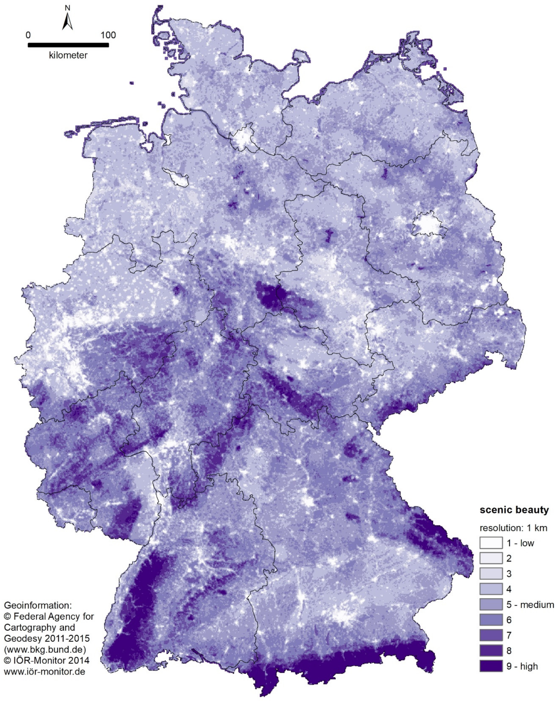
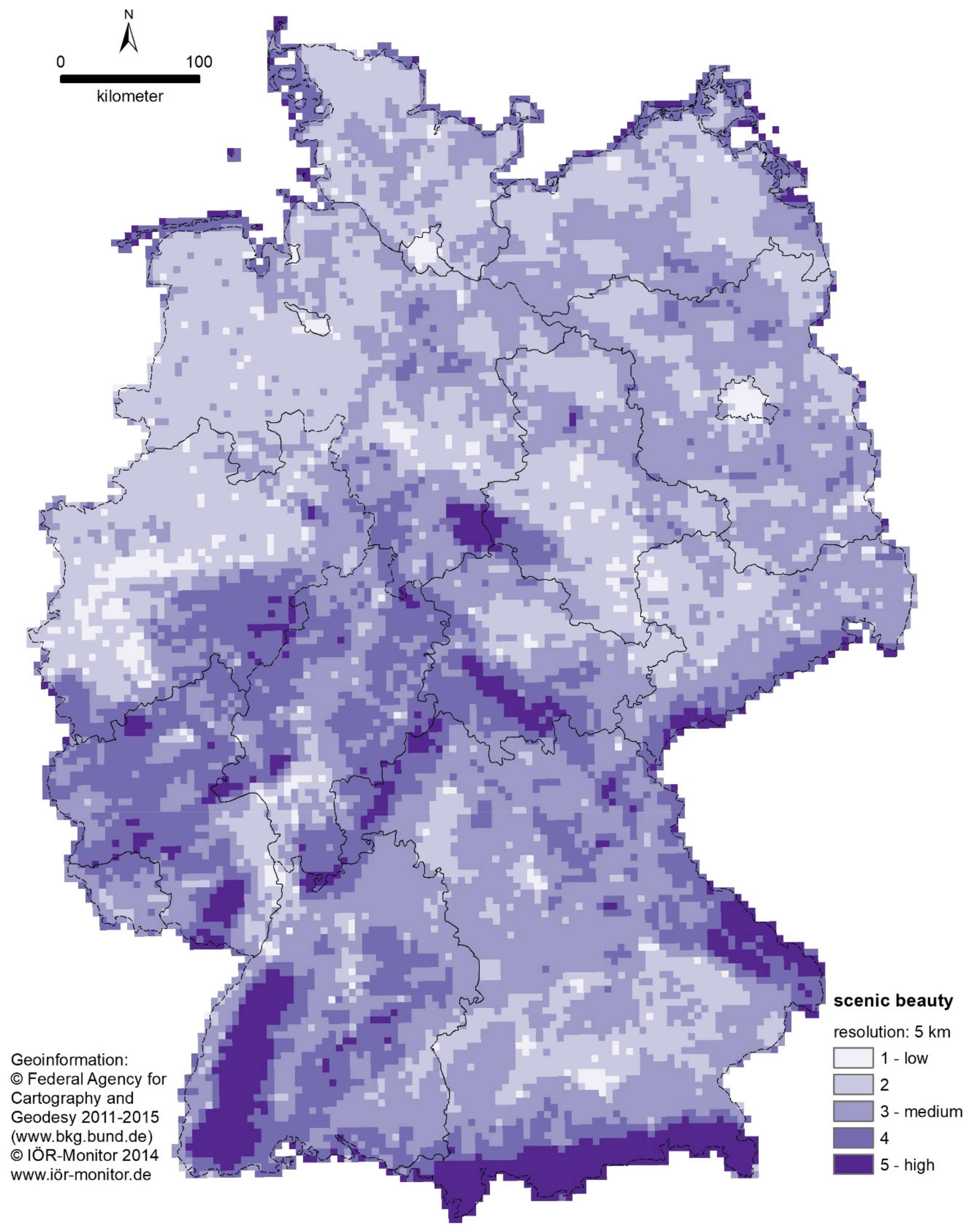
2.2. Assessment of Germany’s Scenic Beauty Based on Online Survey and GIS Data (Method Roth et al.)

The second nationwide visual landscape assessment was conducted in a project financed by the German Federal Agency for Nature Conservation, from 2015 to 2018. Its aim is the use in Strategic Environmental Assessment (SEA) for nationwide grid infrastructure planning. Roth et al. [16] assessed the criteria of visual diversity, landscape character and scenic beauty, separately. In this article, we consider only their assessment of scenic beauty ([16]). By definition, this is closest to the landscape attractiveness assessment (carried out by Walz & Stein [15]), described in the above sections. The indicators in the model for scenic beauty are chosen and weighted based on the results of an online survey using landscape photographs as stimuli. Based on the survey results and geodata in the viewsheds of the landscape photographs, Roth et al. developed a statistical model (regression analysis) for scenic beauty using 30 sampling areas (each around 150 km2) distributed representatively over the German landscapes. Subsequently, the model was applied to the whole study area (Germany).

2.2.1. Underlying Theory

The model for scenic beauty landscape assessment can be classified as a perception-based method [46]. Perception based methods (e.g., [26,28,47,48,49,50,51,52] assume an interaction between the landscape elements (that can be visually perceived) and an observer. The landscape is treated as an objective input to the observer, which is defined by its biophysical components, structures and phenomena. In the online survey, Roth et al. use landscape photographs as a substitute for a real landscape experiences. They also analyse the visible features in the photographs, using GIS Data. The observer’s perception and appreciation of a landscape is affected by biological, cultural and individual factors. The biological factors are—to a great extent—evolutionary determined dispositions, following e.g., the prospect-refugee theory [53,54], the water preference theory [55] or the preference matrix by Kaplan & Kaplan, stating that humans prefer conditions in landscape, which optimize the possibility for gaining knowledge, measured by the four factors legibility, coherence, complexity and mystery [56,57]. The cultural background appears to be a multilayered influence, which may vary across cultural groups and time [58,59,60]. With a nationwide landscape assessment in Germany Roth et al. addressed the subject group of the German population as an example of a typical western culture.

2.2.2. Description of the Approach and Evaluation Method (including Justification of the Choice of Indicators)

In comparison with other existing large-scale landscape assessments, the whole of Germany is a huge study area (about 358,000 km2). To build a representative sample of landscape photographs to use in the online survey, Roth et al. identified 30 sample areas, each around 150 km2 of size. As selection criteria in their two-way stratified sampling, they used the six major regions of the natural landscape classification of Germany [61] and landscape types of Germany defined by Gharadjedaghi et al. [62]. The natural landscape classification of Germany takes into account mainly geological, geomorphical and hydrological features. The Landscape types also represent anthropogenic influences such as human land uses and settlements. Table 3 shows the combinations of the groups of both classifications and the number of sample areas within each combination. The number of sample areas was determined proportionally to the share of area covered by this combination of landscape types and landscape classes within Germany to reach a representative sample of German landscapes covering the maximum diversity of different factors.
Photo documentations were taken in all 30 sample areas, from May to August 2016. Each sample area was visited by car for one day. All photo documentations had to give a representative overview of the different aspects of landscape a sample area exhibits. Different land uses and landscape elements like forest, agriculture, settlements, varying grades of hemeroby, water bodys, roads, wind turbines, power lines etc. have been depicted in different combinations and at different ranges. Over 10,000 photos were taken in total and Roth et al. chose 822 (25 to 30 per sample area) for their online survey.
In the online survey, participants rated the photos on a nine level scale (from 1—not beautiful at all to 9—very beautiful). Roth et al. gave a short definition for the criteria scenic beauty: “the subjective liking of the landscape illustrated in the photograph”. They deliberately kept the definition simple, in order to encourage the participants to apply their own sense of beauty. The question asked to the participants was “How beautiful do you find this landscape?”
To reach a large and representative amount of participants Roth et al. cooperated with a social science online research panel (SoSci Survey). In its two-month duration, 3556 participants took part in the online survey. In total, the participants provided 44,573 ratings, which means that an average of more than 54 ratings per image was achieved. In this methodology, mean values of all ratings for each single photograph were used as dependent variable for the scenic beauty model. For all photos, the exact position, field of view (focal length) and horizontal viewing direction was recorded. Through a GIS-based visibility analysis, based on the national digital elevation model with 10 m resolution (ATKIS-DGM 10), Roth et al. calculated the viewsheds for each landscape photograph. For further analysis they divided the individual viewsheds in several distance zones (Table 4).
Using a GIS, Roth et al. measured about 80 potential indicators, in each distance zone (land uses, landscape elements and landscape metrics). Combining the potential indicators and the various distance zones led to about 600 potential explanatory variables for the linear regression model. A linear regression model uses explanatory variables (regressors) to compute the given values of an explained/dependent variable based on a linear combination of independent variables (cf. [63]). The model shall explain the scenic beauty perceived by the participants based on landscape features within the viewsheds of the landscape photos presented. To build the model Roth et al. used a heuristic, iterative procedure. They tested different combinations of regressor variables until the solution with the highest explanatory power was found.
A raster-based approach was used, as it enables a much faster processing than vector based computations. The smallest possible analysing unit matches distance zone 1. By using the ArcGIS tool “focal statistics” Roth et al. assigned the concept of distance zones illustrated in Table 2 to the raster analysis. Using this approach, raster datasets for all explanatory variables with their associated distance zone for all 365,000 raster cells of the study area (Germany) were calculated. Based on the raster datasets the scenic beauty model was then applied to the whole of Germany. The outcome of the raster analysis is a nationwide scenic quality map.

2.2.3. Data Used

For a nationwide assessment, the aim was to use geo data of homogeneous quality for the whole of Germany. Extensive land covers were taken from the Land Cover Model for Germany (LBM-DE). They used the land cover classes provided by the LBM-DE as indicators by themselves and furthermore formed groups of related classes. To illustrate this using an example, the classes “broadleaf forest (311)”, “conifer forest (312)” and “mixed forest (313)” were analysed individually and combined as the land cover group “forest”. For linear elements like power lines and streets, the German Digital Landscape Model (ATKIS-Base-DLM) was used. Single elements were extracted from the OpenStreetMap Dataset. Roth et al. also used the nationwide hemeroby dataset of the Leibniz Institute of Ecological Urban and Regional Development [41] and the already mentioned ATKIS-DGM 10 as a digital elevation model (DEM) to take into account the relief.

2.2.4. Resolution, Raster Width of the Grid

After successful model building, Roth et al. determined the occurrence of each indicator, which was used as explanatory variable, in a 1-km raster nationwide. Since the aim of the nationwide scenic beauty assessment was its use in the Strategic Environmenal Assessment (SEA) for the nationwide grid infrastructure planning, a relatively fine resolution was desirable. The 1-km resolution is a compromise between accuracy and computing time needed to process the data.

2.2.5. Empirically Based Weighting of Indicators in the Regression Analysis

Table 5 shows the results of the linear regression used to build the scenic beauty model. It lists all explanatory variables with their appropriated distance zone and non-standardized as well as standardized beta coefficients. With a coefficient of determination (r2) of 0.639 the model explains about 64% of the variance in the mean photo ratings for scenic beauty. The model contains 17 explanatory variables. A high positive influence on scenic beauty can be found for the relief (measured by difference in ground level) and the occurrence of water bodies. Forest and other green and natural-appearing land uses have also a positive effect. An indicator that led to explicitly high scenic beauty ratings in photos was the occurrence of heathlands. However, regressors with a negative impact make up the larger part of the model. The major regressor here is hemeroby, the level of anthropogenic influence. Consistent with that effect, land uses and landscape elements, which are clearly signs of human use of landscape are negatively weighted. This applies to traffic infrastructure, industrial areas and arable land. In addition, technical infrastructure like transmission lines and wind turbines have a negative effect.

2.2.6. Correlation of the Parameters with Each Other

To ensure the independence of the regressor variables, it was a requirement that an indicator does not occur multiple time in a distance zone (e.g., in zone 1 and foreground) or individually and in a group of land cover classes. Furthermore, through the iterative approach, the least possible thematic overlap of the explanatory variables was ensured. In addition, it was screened, that there are no strong correlations between regressors to avoid multi-collinearity.

2.2.7. Classification

Following the nine-step scale of the online survey, the method aimed at assigning a nine-class scale to the outcome raster. In some raster cells, the outcome values in the regression model exceeded the values of the nine-step online survey scale. Thus, a reclassification of the values calculated by the regression model was performed, using a scheme whose class breaks are linked to mean value (MV) and standard deviation (SD) (cf. Table 6).

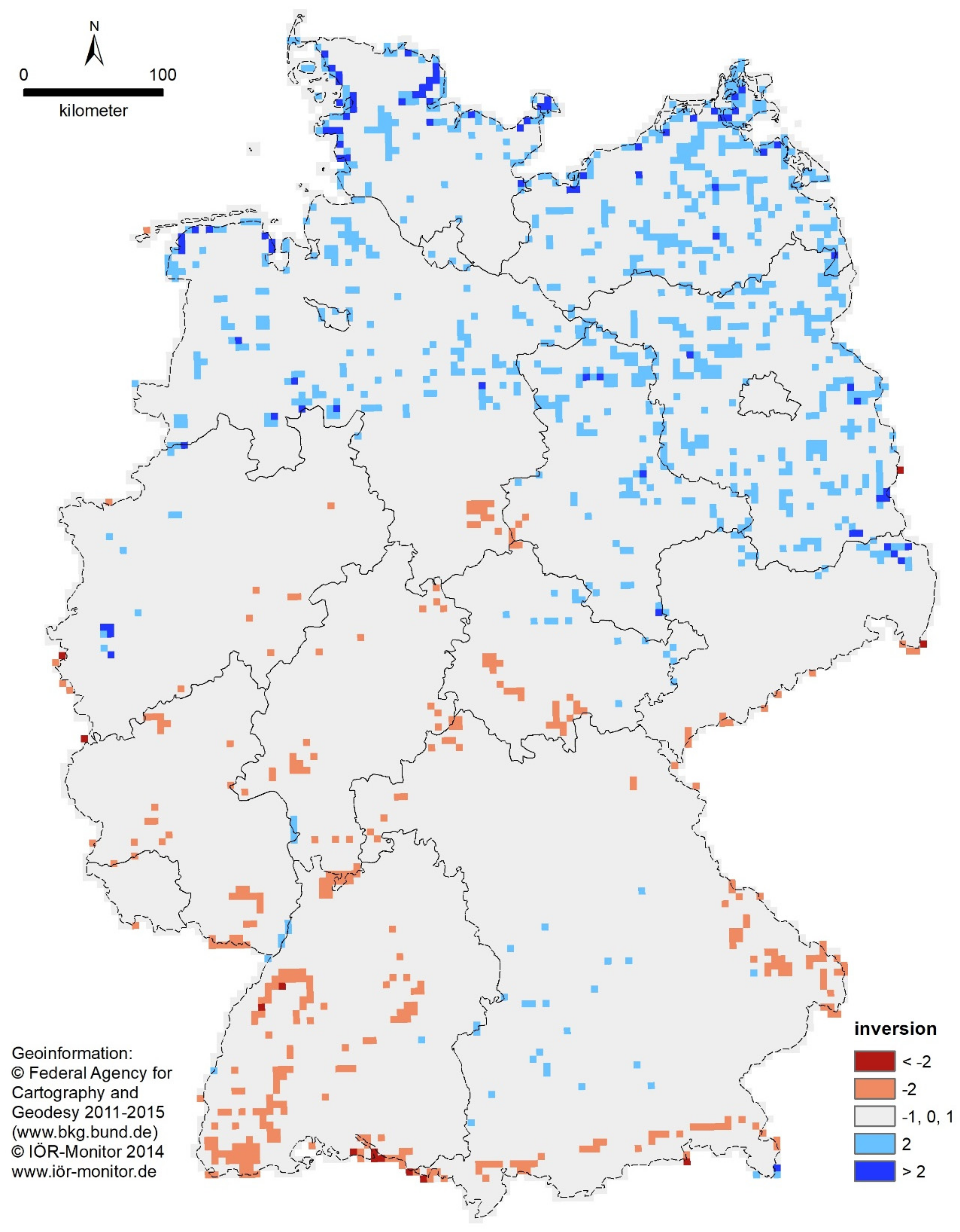
2.3. Method for Comparison of the Two Large-Area Visual Landscape Assessments

To compare the results of the two methods described above, we use the cardinally scaled outcome raster of the respective methods, prior to the assignment of any classes. As a spatial reference base, we choose the INSPIRE 5-km-grid of the model for landscape attractivity (Walz & Stein) presented first. As first step we projected the outcome raster of the scenic beauty model (Roth et al.) to the coordinate system of the reference raster. We then transferred the 1-km raster applied in the scenic beauty assessment to the 5-km raster applied in the landscape attractiveness method, by aggregating mean values of the finer resolution to the zones defined by the coarser resolution. This was done to have the same spatial basis and resolution to enable statistical comparisons. The overlay of the two visual landscape assessments was then exported to SPSS to determine correlation (Pearson’s r) between the two datasets. To visualize similarities and differences we applied the same classification scheme used for the landscape attractivity assessment of Walz & Stein [15] to the newly created 5-km raster for scenic beauty. We compared the two 5-class assessments directly by subtracting the values of one raster from the other to generate an inversion display.

3. Results

3.1. Landscape Attractiveness Assessment Results (Method Walz & Stein)

With its diverse cultural and natural landscapes, Germany is very varied and scenically attractive (see Figure 1). The classes “very attractive” and “particularly attractive” describe landscapes that stand out in their diversity and characteristics and are therefore much more attractive than the national German average. These are above all areas on the coasts, in the Alps and in wooded low mountain ranges such as the Black Forest, the Palatinate Forest, the Thuringian Forest, the Harz, the Ore Mountains and others. The relief, the closeness to nature and the particular attractiveness of the coast are particularly evident here. In addition, parts of the north (east) German lowlands with little relief but with a high proportion of lakes and forests in Brandenburg and Mecklenburg-Western Pomerania were also rated very highly. These landscapes, classified as very or particularly attractive, largely coincide with the nationally known destinations for nature-related tourism and the holiday regions.
In the “average attractive” class, there are landscapes which, viewed across Germany, show a typical characteristic of the diversity and landscape structure of Central European landscapes. They are quite attractive, but the outstanding properties are missing. There are many traditional cultural landscapes, which can also be holiday regions, but in particular fulfil local recreational functions. Examples are the Swabian-Franconian Alb, parts of the Rhenish Slate Mountains or the Hessian mountainous region. In the “less attractive” class there are mostly structurally poor, above all intensively agriculturally used areas and metropolitan areas. “Least attractive” landscapes are characterized by low values for all seven parameters, which is an indication of dense development (e.g., in densely populated areas such as the Ruhr area, the Middle Neckar around Stuttgart or in the Berlin area) or low naturalness of land use, e.g., intensive agriculture. Examples of this are the Loessbörden of Lower Saxony, Saxony-Anhalt and Saxony, but also the Lower Bavarian hill country. High densities of technical systems, such as wind turbines, high-voltage lines, etc. can also lead to a reduction in the values.

3.2. Scenic Beauty Assessment Results (Method Roth et al.)

Roth et al. applied the linear regression model described above to the area of Germany and displayed the outcome as a map, dividing scenic beauty on a nine-level-scale (Figure 2). The strong positive effect of relief, water bodies and forest as well as the strong negative impact of anthropogenic influence in the landscape shows clearly on the map. The highest levels 8 and 9 (coloured dark) are assigned to regions like the Harz Mountains, Thuringian Forest, Black Forest, Bavarian Forest and the Alps, which are characterized by steep relief, semi-natural land uses and minor presence of anthropogenic elements in the landscape (Figure 3). Also regions, rich in water reach high levels of 7 and 8 (e.g., Mecklenburg Lake District, North and Baltic Sea Coast) (Figure 4). Urban Agglomerations and urbanized regions, with high amounts of traffic infrastructure (e.g., big cities like Berlin, Hamburg or Munich and their surroundings) are assessed particularly negative. Likewise regions with high occurrence of industry and a corresponding high settlement and traffic infrastructure density (e.g., the Ruhr agglomeration) are assigned low values for scenic beauty (Figure 5). Areas with intensive agriculture can also be identified through lower values, especially if they contain a high amount of wind turbines and power lines (cf. e.g., the Magdeburg Börde) (Figure 6).

3.3. Comparison of the Two Large Area Visual Landscape Assessments

As has been described above, in order to compare the results of the two assessments, we transferred them to the same spatial reference system and brought them to the same resolution of the 5-km INSPIRE grid. We calculated the correlation between the two assessment values for each grid cell based on the raw outcome values of the respective methods (not the classified values). A correlation of Pearson’s r = 0.772 (r2 = 0.596, p < 0.001) could be observed. Taking into account that both methods represent the average individual subjective appreciation of visual landscape quality, which is a complex psychological process and only partially based on the presence of objective landscape elements, we use thresholds from social science literature [63], psychology [64] and geography [65] to interpret the strength of this correlation. From a social sciences and psychology perspective, a value of r > 0.5 can be classified as a strong effect, whereas from a geographical perspective, a value of 0.6 < r < 0.8 would be classified as a distinct effect (and values of r > 0.8 as a strong effect).
To be able to contrast both assessments visually, we divided the newly generated cardinally scaled outcome raster for scenic beauty with 5-km resolution in 5 classes (Figure 7) to have both the same spatial reference system (see above) and the same classification system.
The map in Figure 8 shows the inversions, generated by subtracting the raster values of the scenic beauty dataset from the landscape attractiveness values (Walz & Stein-Roth et al.). Thus negative values (red raster cells) reveal areas, where the scenic beauty assessment by Roth et al. [16] scored higher and positive values (blue raster cells) show areas where the landscape attractiveness of Walz & Stein [15]) has higher values. Table 7 shows the frequency of inversion values. In about 91% of all raster cells, there was no difference in the classified assessement or the difference was only one level (on a 5 level ordinal scale). Differences of 3 or 4 level are very rare (<1%).

4. Discussion

First of all, it should be noted that the two models lead to valid and reliable results and thus agree to a large extent. It becomes clear that the landscape attractiveness assessment by Walz & Stein [15] scored a little bit higher values in the north of Germany and the scenic beauty assessment by Roth et al. [16] tends to score little higher values in some few parts of central and southern Germany. Main reasons for these differences could be that with the approach Roth et al. [16] (scenic beauty model), the relief (differences in ground level, topographic diversity) plays a major role (relief in fore- and background were the highest weighted regressors), whereas the approach by Walz & Stein [15] weighted indicators equally. Thus, regions of Germany’s up- and highlands areas are partially marked in red in the inversion map. Terrain is not only such a relevant factor (and good predictor of scenic quality) because undulating terrain provides vistas and viewers appreciate long distance lookouts over varied surfaces, but also because many secondary factors depend on terrain. This applies for example to the intensity and parcel size of agricultural uses, which tends to be less intense and on a smaller mosaic in steeper terrain and higher altitudes.
Blue areas (rated higher by the landscape attractiveness assessment by Walz & Stein [15]) are often regions, which are rich in water (e.g., the lake districts in the federal states Mecklenburg-Western Pomerania and Brandenburg, as well as the coastal area). Despite the fact that waterbodies were one of the regressors with the highest positive weight in the scenic beauty model by Roth et al. [16], Walz & Stein [15] gave them an even higher relative weight by equally weighting all indicators.
Generally speaking, some of the indicators used by the two methods were congruent (e.g., the hemeroby indicator). Others were similar but different (e.g., the way terrain was represented in the two models), while some were only present in one model (e.g., the percentage of open space used by Walz & Stein [15], or the heathlands and road density used by Roth et al. [16]).
One fundamental difference is that the scenic beauty assessment by Roth et al. [16] is based on an empirical survey and a statistical modelling approach, which allows to assess the model quality by the coefficient of determination (r2). In contrast, the landscape attractiveness method is based on the normative setting of equal weights for all indicators used. Yet, by triangulating the two methods described in this paper, an additional external validation approach is performed for both methods. The fact that despite the theoretical, methodical and empirical differences, a correlation of Pearson’s r = 0.772 (r2 = 0.596, p = 0.000) could be observed, shows that a large and common share of visual landscape qualities can be explained by objective geodata on landscape elements, land uses and landscape metrics.
The two approaches differ in the spatial resolution (1 km with Roth et al. [16] and 5 km with Walz & Stein [15]). This leads to different effects: Whereas the finer resolution allows to clearly see narrower river valleys such as the Danube valley in Southern Germany or the Elbe valley in Northern Germany, the coastal zones with high visual quality are better represented in the approach using the coarser resolution).
Another difference in the methodological approaches that is partly due to the different resolutions is that Walz & Stein [15] restricted the indicators relevant for a raster cell to those geodata occurring in this cell. Roth et al. [16] in contrast analysed the indicators in several distance zones around the cell to be assessed in addition to the geodata occurring in this specific cell.
Both datasets can be used for a regular monitoring of landscape quality, by re-assessing the German landscape with updated geodata (changed land uses, new or lost landscape elements, and different landscape metrics). The scenic beauty assessment by Roth et al. [16] also allows including changed value systems in the landscape viewers’ assessment into the method. This can be done by replicating the survey and then giving modified weights to the indicators, based on a new statistical modelling of the regression analysis. A suitable timeframe/interval for the repetition based on modified geodata might start from 3–5 years, whereas the repetition based on changed value systems requires a longer perspective (such as 5–10 years minimum), because the value shifts are slower processes. For the ease of communication with decision-makers, it might make sense to aggregate the resulting data for administrative units such as municipalities, which Walz & Stein [15] have already done.

5. Conclusions and Outlook

The main conclusion of this paper is that a valid visual landscape quality assessment for large areas is possible, and that the quality of these assessment methods/models can be empirically proven by method triangulation. While both approaches investigated are not congruent but cover different aspects of visual landscape quality (and were developed for a different purpose), both can be used as a benchmarking for regional/local assessment to contextualize them within a larger landscape setting. Yet, the following, more detailed levels of planning have to add more detailed data that is relevant on the local and regional level.
During and after the development of the two approaches, a very high demand from the planning practice for these nationwide datasets could be observed. Thus, we are confident, that by providing these datasets to the practice, gaps of a rudimentary assessment or risks of underestimating the visual landscape quality in high-level planning procedures, such as for the Federal Transport Infrastructure Plan or for the expansion of the federal electricity grid, could be avoided. Yet, it cannot always be taken for granted that the political acceptance of these assessments can be ensured. Nevertheless, we are confident that a methodologically sound, validated visual landscape assessment, especially if based on or validated by representative empirical data (which could also be classified as a kind of citizen science approach), has a much better standing and can withstand also better at court, than a single expert’s assessment.
From an academic perspective, the continuous advance of spatial modelling in the field of visual landscape assessment is a prospective research area, knowing that the complexity of the methods used, the amount of data analysed, and the computation power required cannot be provided in standard planning applications by the practitioners themselves. Thus, this paper shall also contribute to raising the awareness about what is technically possible, which is an underutilized potential [66].

Author Contributions

Conceptualization, M.R. and W.W.; methodology, M.R. and W.W.; validation, M.R.; formal analysis, S.H. and U.W.; data curation, S.H. and U.W.; writing—original draft preparations, M.R., S.H., U.W. and W.W.; writing—review and editing, M.R., S.H., U.W. and W.W.; supervision, M.R. All authors have read and agreed to the published version of the manuscript.

Funding

This research was funded by the German Federal Agency for Nature Conservation (Bundesamt für Naturschutz–BfN), grant number FKZ 3515 82 2800, and by the German Research Foundation (Deutsche Forschungsgemeinschaft–DFG), grant number WE 3057/3-1 resp. WA 2131/2-1.

Institutional Review Board Statement

Not applicable.

Informed Consent Statement

Not applicable.

Data Availability Statement

Not applicable.

Conflicts of Interest

The authors declare no conflict of interest.

References

  1. European Commission. COUNCIL DIRECTIVE 92/43/EEC of 21 May 1992 on the Conservation of Natural Habitats and of Wild Fauna and Flora. Available online: https://eur-lex.europa.eu/legal-content/EN/TXT/PDF/?uri=CELEX:31992L0043&from=EN (accessed on 15 October 2020).
  2. European Commission. Green Infrastructure (GI)—Enhancing Europe’s Natural Capital—COM (2013) 149. Available online: https://eur-lex.europa.eu/resource.html?uri=cellar:d41348f2-01d5-4abe-b817-4c73e6f1b2df.0014.03/DOC_1&format=PDF (accessed on 15 October 2020).
  3. Ellwanger, G.; Ssymank, A. Managementpläne für Natura-2000-Gebiete. In Landschaftsplanung, 3rd ed.; Riedel, W., Lange, H., Jedicke, H., Reinke, M., Eds.; Springer Spektrum: Berlin/Heidelberg, Germany, 2016; pp. 305–314. [Google Scholar] [CrossRef]
  4. Federal Agency for Nature Conservation Germany. Federal Green Infrastructure Concept. Available online: https://www.bfn.de/fileadmin/BfN/planung/bkgi/Dokumente/BKGI_Broschuere_englisch.pdf (accessed on 15 October 2020).
  5. Wende, W.; Hanusch, M.; Gassner, E.; Guennewig, D.; Koeppel, J.; Lambrecht, H.; Langenheld, A.; Peters, W.; Roethke-Habeck, P. Requirements of the SEA Directive and the German Federal Transport Infrastructure Plan. Europ. Env. 2004, 14, 105–122. [Google Scholar] [CrossRef]
  6. Rehhausen, A.; Köppel, J.; Scholles, F.; Stemmer, B.; Syrbe, R.-U.; Magel, I.; Geißler, G.; Wende, W. Quality of federal level strategic environmental assessment—A case study analysis for transport, transmission grid and maritime spatial planning in Germany. Env. Imp. Assessm. Rev. 2018, 73, 41–59. [Google Scholar] [CrossRef]
  7. Hersperger, A.-M.; Bürgi, M.; Wende, W.; Bacău, S.; Grădinaru, S.-R. Does landscape play a role in strategic spatial planning of European urban regions? Landsc. Urban Plan. 2020, 194, 103702. [Google Scholar] [CrossRef]
  8. Wende, W.; Walz, U.; Stein, C. Evaluating municipal landscape plans and their influence on selected aspects of landscape development—An empirical study from Germany. Land Use Policy 2020, 99, 104855. [Google Scholar] [CrossRef]
  9. Monitor of Settlement and Open Space Development (IOER Monitor). Available online: https://www.ioer-monitor.de/en/ (accessed on 15 October 2020).
  10. Robert, S. Assessing the visual landscape potential of coastal territories for spatial planning. A case study in the French Mediterranean. Land Use Policy 2018, 72, 138–151. [Google Scholar] [CrossRef]
  11. Sklenicka, P.; Zouhar, J. Predicting the visual impact of onshore wind farms via landscape indices: A method for objectivizing planning and decision processes. Appl. Energy 2018, 209, 445–454. [Google Scholar] [CrossRef]
  12. Schmid, W. The emerging role of visual resource assessment and visualisation in landscape planning in Switzerland. Landsc. Urban Plan. 2001, 54, 213–221. [Google Scholar] [CrossRef]
  13. Roth, M.; Bruns, E. Landschaftsbildbewertung in der vorsorgenden Landschaftsplanung—Stand und Perspektiven. Natur Landsch. 2016, 91, 537–543. [Google Scholar] [CrossRef]
  14. Hildebrandt, S.; Roth, M. Landschaftsbildbewertung auf Landesebene—Stand und Eignung gängiger Verfahren. Nat. Schutz Landsch. Plan 2020, 52, 62–67. [Google Scholar]
  15. Walz, U.; Stein, C. Indicator for a monitoring of Germany’s landscape attractiveness. Ecol. Indic. 2018, 94, 64–73. [Google Scholar] [CrossRef]
  16. Roth, M.; Hildebrandt, S.; Röhner, S.; Tilk, C.; Schwarz-von Raumer, H.G.; Roser, F.; Borsdorff, M. Landscape as an area as perceived by people: Empirically-based nationwide modelling of scenic landscape quality in Germany. J. Digit. Landsc. Archit. 2018, 3, 129–137. [Google Scholar] [CrossRef]
  17. Council of Europe. European Landscape Convention. 2000. Available online: https://rm.coe.int/1680080621 (accessed on 27 January 2021).
  18. Kiemstedt, H. Zur Bewertung der Landschaft für die Erholung; Ulmer: Hannover, Germany, 1967. [Google Scholar]
  19. Briggs, D.J.; France, J. Assessing landscape attractiveness: A South Yorkshire study. Landsc. Res. 1981, 6, 2–5. [Google Scholar] [CrossRef]
  20. Marks, R. Erholungsfunktion. In Anleitung zur Bewertung des Leistungsvermögens des Landschaftshaushaltes; Marks, R., Müller, M.J., Leser, H., Klink, H.-J., Eds.; Zentralausschuß für dt. Landeskunde: Trier, Germany, 1989; pp. 129–136. ISBN 3-88143-030-X. [Google Scholar]
  21. Chen, Y.-L.; Maier, J.; Menchen, N.; Sieker, T.; Stoiber, M. Fremdenverkehrsgebiete und naturräumliche Ausstattung. In Freizeit und Tourismus; Spektrum Akademischer Verlag: Heidelberg, Germany, 2000; ISBN 3827409381. [Google Scholar]
  22. Augenstein, I. Die Ästhetik der Landschaft. In Ein Bewertungsverfahren für die Planerische Umweltvorsorge; Weißensee Verlag: Berlin, Germany, 2002; ISBN 3934479901. [Google Scholar]
  23. Berger, A.; Walz, U. Landschaftsmaße für eine Langzeituntersuchung von Flächennutzungsänderungen in Ostsachsen. In Landschaftsstruktur im Kontext von Naturräumlicher Vorprägung und Nutzung—Datengrundlagen, Methoden und Anwendungen; Walz, U., Lutze, G., Schultz, A., Syrbe, R.-U., Eds.; Leibniz-Institut für ökologische Raumentwicklung Dresden (IÖR): Dresden, Germany, 2004; pp. 255–272. ISBN 3933053242. [Google Scholar]
  24. Federal Office for Building and Regional Planning (BBR—Bundesamt für Bauwesen und Raumordnung). Raumordnungsbericht; BBR: Bonn, Germany, 2005; ISBN 3879940711. [Google Scholar]
  25. Roth, M.; Gruehn, D. Modellierung von Vielfalt, Eigenart und Schönheit von Natur und Landschaft: Kriterien zur Bestimmung von Landschaftsbildqualitäten für große Räume. Nat. Schutz Landsch. Plan. 2010, 42, 115–120. [Google Scholar]
  26. Roth, M.; Gruehn, D. Visual Landscape Assessment for Large Areas—Using GIS, Internet Surveys and Statistical Methodologies in Participatory Landscape Planning for the Federal State of Mecklenburg-Western Pomerania, Germany. Proc. Latv. Acad. Sci. Sect. Hum. Soc. Sci. 2012, 66, 129–142. [Google Scholar]
  27. Frank, S.; Fürst, C.; Koschke, L.; Witt, A.; Makeschin, F. Assessment of landscape aesthetics—Validation of a landscape metrics-based assessment by visual estimation of the scenic beauty. Ecol. Indic. 2013, 32, 222–231. [Google Scholar] [CrossRef]
  28. Schirpke, U.; Tasser, E.; Tappeiner, U. Predicting scenic beauty of mountain regions. Landsc. Urban Plan. 2013, 111, 1–12. [Google Scholar] [CrossRef]
  29. Schüpbach, B.; Junge, X.; Lindemann-Matthies, P.; Walter, T. Seasonality, diversity and aesthetic valuation of landscape plots: An integrative approach to assess landscape quality on different scales. Land Use Policy 2016, 53, 27–35. [Google Scholar] [CrossRef]
  30. Hermes, J.; Albert, C.; Von Haaren, C. Assessing the aesthetic quality of landscapes in Germany. Ecosyst. Serv. 2018, 31, 296–307. [Google Scholar] [CrossRef]
  31. Roth, M.; Bruns, E. Landschaftsbildbewertung in Deutschland—Stand von Wissenschaft und Praxis: Ergebnisse eines Sachverständigengutachtens im Auftrag des Bundesamtes für Naturschutz; Bundesamt für Naturschutz: Bonn-Bad Godesberg, Germany, 2016. [Google Scholar]
  32. Stein, C.; Walz, U. Indikator für ein Monitoring der landschaftlichen Attraktivität Deutschlands. In Flächeninanspruchnahme in Deutschland: Auf dem Wege zu Einem Besseren Verständnis der Siedlungs-und Verkehrsflächenentwicklung; Behnisch, M., Kretschmer, O., Meinel, G., Eds.; Springer Spektrum: Berlin, Germany, 2018; pp. 155–169. ISBN 9783662503041. [Google Scholar]
  33. Nohl, W. Heimat als symbolischer Aneignungsprozess—Konzeptionelle Überlegungen und empirische Untersuchungen. Nat. Schutz Landsch. Plan. 2006, 38, 140–145. [Google Scholar]
  34. Gailing, L.; Leibenath, M. (Eds.) Neue Energielandschaften—Neue Perspektiven der Landschaftsforschung; Springer Fachmedien: Wiesbaden, Germany, 2013; ISBN 978-3-531-19794-4. [Google Scholar]
  35. Walz, U. Indicators to monitor the structural diversity of landscapes. Ecol. Model. 2015, 295, 88–106. [Google Scholar] [CrossRef]
  36. Walz, U.; Berger, A. Analyse der Auswirkungen des Landschaftswandels auf die Erholungseignung. In Angewandte Geoinformatik 2004: Beiträge zum 16. AGIT-Symposium Salzburg; Strobl, J., Blaschke, T., Griesebner, G., Eds.; Wichmann: Heidelberg, Germany, 2004; pp. 760–769. ISBN 9783879074068. [Google Scholar]
  37. Freiraum und Naturschutz: Die Wirkungen von Störungen und Zerschneidungen in der Landschaft; Baier, H.; Erdmann, F.; Holz, R.; Waterstraat, A. (Eds.) Springer: Berlin/Heidelberg, Germany, 2006; ISBN 978-3-540-30824-9. [Google Scholar]
  38. Nohl, W. Grünland und Landschaftsästhetik. Die ästhetische Bedeutung von Grünland und die Auswirkungen vermehrten Grünlandumbruchs auf das Landschaftsbild. Nat. Landsch. 2009, 41, 357–364. [Google Scholar]
  39. Coeterier, J.F. Dominant attributes in the perception and evaluation of the Dutch landscape. Landsc. Urban. Plan. 1996, 34, 27–44. [Google Scholar] [CrossRef]
  40. Real, E.; Arce, C.; Manuel Sabucedo, J. Classification of Landscapes using quantitative and categorical data, and prediction of their scenic beauty in north-western Spain. J. Environ. Psychol. 2000, 20, 355–373. [Google Scholar] [CrossRef]
  41. Walz, U.; Stein, C. Indicators of hemeroby for the monitoring of landscapes in Germany. J. Nat. Conserv. 2014, 22, 279–289. [Google Scholar] [CrossRef]
  42. Nohl, W. Sustainable landscape use and aesthetic perception—preliminary reflections on future landscape aesthetics. Landsc. Urban Plan. 2001, 54, 223–237. [Google Scholar] [CrossRef]
  43. Kienast, F.; Degenhardt, B.; Weilenmann, B.; Wäger, Y.; Buchecker, M. GIS-assisted mapping of landscape suitability for nearby recreation. Landsc. Urban Plan. 2012, 105, 385–399. [Google Scholar] [CrossRef]
  44. Walz, U. Verwendung von Landschaftsstrukturmaßen zur Analyse und Bewertung der biologischen Vielfalt von Landschaften. Arch. Forstwes. Landsch. 2011, 45, 116–130. [Google Scholar]
  45. Koldrack, N.; Bill, R.; Walz, U. GIS-basierte Ermittlung der Flächeninanspruchnahme für Energieinfrastrukturen in Deutschland. GIS Sci. 2014, 2, 55–63. [Google Scholar]
  46. Daniel, T.C. Whither Scenic beauty? Visual landscape quality assessment in the 21st century. Landsc. Urban Plan. 2001, 54, 267–281. [Google Scholar] [CrossRef]
  47. Bishop, I.D.; Hulse, D.W. Prediction of scenic beauty using mapped data and geographic information systems. Landsc. Urban Plan. 1994, 30, 59–70. [Google Scholar] [CrossRef]
  48. Palmer, J.F.; Lankhorst, J.R.K. Evaluating visible spatial diversity in the landscape. Landsc. Urban Plan. 1998, 43, 65–78. [Google Scholar] [CrossRef]
  49. Hunziker, M.; Kienast, F. Potential impacts of changing agricultural activities on scenic beauty—A prototypical technique for automated rapid assessment. Landsc. Ecol. 1999, 14, 161–176. [Google Scholar] [CrossRef]
  50. Bishop, I.D.; Wherrett, J.R.; Miller, D.R. Using image depth variables as predictors of visual quality. Environ. Plan. B Plan. Des. 2000, 27, 865–875. [Google Scholar] [CrossRef]
  51. Roth, M.; Gruehn, D. Scenic quality modelling in real and virtual environments. In Trends in Real Time Landscape Visualization and Participation; Buhmann, E., Paar, P., Bishop, I.D., Lange, E., Eds.; Wichmann-Verlag: Heidelberg, Germany, 2005; pp. 291–302. [Google Scholar]
  52. Roser, F. Entwicklung einer Methode zur Großflächigen RECHNERGESTÜTZTEN Analyse des Landschaftsästhetischen Potenzials; Weißensee Verlag: Berlin, Germany, 2011. [Google Scholar]
  53. Appleton, J. Propects and refuges revisited. Landsc. J. 1984, 8, 91–103. [Google Scholar] [CrossRef]
  54. Appleton, J. The Experience of Landscape; Wiley: Chichester, UK, 1996; ISBN 978-0471032564. [Google Scholar]
  55. Bourassa, S.C. The Aesthetics of Landscape; Belhaven Press: London, UK, 1991; ISBN 978-1852930714. [Google Scholar]
  56. Kaplan, S. Aesthetics, affect, and cognition: Environmental preferences from an evolutionary perspective. Environ. Behav. 1987, 19, 3–32. [Google Scholar] [CrossRef] [Green Version]
  57. Kaplan, R.; Kaplan, S. The Experience of Nature: A Psychological Perspective; Cambridge University Press: Cambridge, UK, 1989; ISBN 978-0521341394. [Google Scholar]
  58. Buyhoff, G.J.; Wellmann, J.D.; Koch, N.E.; Gauthier, L.; Hultman, S. Landscape preference metrics: An international comparison. J. Environ. Manag. 1983, 16, 181–190. [Google Scholar]
  59. Yang, B.E.; Kaplan, R. The perception of landscape style: Across-cultural comparison. Landsc. Urban Plan. 1990, 19, 251–262. [Google Scholar]
  60. Jacobs, M. Psychology of the Visual Landscape. In Exploring the Visual Landscape; Advances in Physiognomic Landscape Research in the Netherlands. Research in Urbanism Series; Nijhuis, S., Lammeren, R.V., Hoeven, F.V.D., Eds.; IOS Press: Amsterdam, The Netherlands, 2011; Volume 2, pp. 41–54. [Google Scholar]
  61. Meynen, E.; Schmithüsen, J.; Gellert, J.; Neef, E.; Müller-Miny, H.; Schulze, J.H. Handbuch der Naturräumlichen Gliederung Deutschlands; Bundesanstalt für Landeskunde und Raumforschung: Bad Godesberg, Germany, 1962. [Google Scholar]
  62. Gharadjedaghi, B.; Heimann, R.; Lenz, K.; Martin, C.; Pieper, V.; Schulz, A.; Riecken, U. Verbreitung und Gefährdung schutzwürdiger Landschaften in Deutschland. Natur Landsch. 2004, 79, 71–81. [Google Scholar]
  63. Bortz, J.; Schuster, C. Statistik für Human-und Sozialwissenschaftler, 7th ed.; Springer: Berlin, Germany, 2010; ISBN 978-3642127694. [Google Scholar]
  64. Cohen, J. A power primer. Psychol. Bull. 1992, 112, 155. [Google Scholar] [CrossRef]
  65. Zimmermann-Janschitz, S. Statistik in der Geographie: Eine Exkursion Durch die Deskriptive Statistik; Springer Spektrum: Berlin, Germany, 2014; ISBN 978-3-8274-2612-3. [Google Scholar]
  66. Liu, M.; Nijhuis, S. Mapping landscape spaces: Methods for understanding spatial-visual characteristics in landscape design. Environ. Impact Assess. Rev. 2020, 82, 106376. [Google Scholar] [CrossRef]
Figure 1. Landscape attractiveness in Germany (method Walz & Stein), using a 5-km-grid.
Sustainability 13 01891 g001
Figure 2. Resulting map for scenic beauty of Germany based on linear regression (resolution: 1 × 1 km) by Roth et al. [16].
Sustainability 13 01891 g002
Figure 3. Landscapes with varieties in relief and uncommon sights like heathland belong to the most appreciated landscape photos in the online survey and lead to high levels in scenic beauty assessment (left: Alps near Oberammergau, Bavaria, right: Lueneburg Heath near Hermannsburg, Lower Saxony).
Sustainability 13 01891 g003
Figure 4. Landscapes dominated by water are preferred, especially when paired with forest and greenways (left: coastal area of North Sea near Nordholz, Lower Saxony, right: lake near Wilhelmsdorf, Baden-Württemberg).
Sustainability 13 01891 g004
Figure 5. Densely populated regions reached low levels in online survey and model results, especially if they are rich in industry and transport infrastructure (left: Ingelheim, Rhineland-Palatinate, right: Gelsenkirchen, North Rhine-Westphalia).
Sustainability 13 01891 g005
Figure 6. Unstructured agricultural landscapes often come with energy infrastructure like power lines and wind turbines and are not considered scenically beautiful (left: agricultural area with grid infrastructure near Magdeburg, Saxony-Anhalt, right: agricultural area with wind turbines near Hermannsburg, Lower Saxony).
Sustainability 13 01891 g006
Figure 7. Resulting map of scenic beauty assessment (Roth et al.) with a resolution of 5 × 5 km.
Sustainability 13 01891 g007
Figure 8. Inversions as visualization for comparison between the two large visual landscape assessments. Red values show a higher score by Roth et al. [16] (scenic beauty assessment) and blue value imply a higher score by Walz & Stein [15] (landscape attractiveness assessment).
Sustainability 13 01891 g008
Table 1. Correlation matrix of all parameters; N = 14,859 (Pearson’s r), all correlations are significant at the level of 0.05. Source: [15].
Proportion of Unfragmented Open Space > 50 km2Topographic Diversity Ratio of Riparian AreasDensity of Ecotones Dominated by Woody PlantsHemeroby IndexPercentage of Open SpaceCoastlinesCharacterising Impacts of Technical Infrastructure
Wind TurbinesPhotovoltaic Power PlantsHigh-Voltage Power Lines
Proportion of unfragmented open space > 50 km21.0000.2260.094−0.1150.3990.2480.1710.0560.0150.209
Topographic diversity0.2261.000−0.0270.0770.4030.107−0.0650.0870.0300.093
Ratio of riparian areas0.094−0.0271.000−0.0250.0650.0340.180−0.0410.0280.042
Density of ecotones dominated by woody plants−0.1150.077−0.0251.0000.033−0.117−0.1020.0660.031−0.022
Hemeroby index0.3990.4030.065−0.0331.0000.4910.3060.1720.0530.312
Percentage of open space0.2480.1070.034−0.1170.4911.0000.012−0.0710.0210.230
Coastlines0.171−0.0650.180−0.1020.3060.0121.000−0.0210.0210.111
Caracterising impacts of technical infrastructureWind turbines0.0560.087−0.0410.0660.172−0.071−0.0211.0000.0040.037
Photo-voltaic power-plants0.0150.0300.0280.0310.0530.0210.0210.0041.0000.030
High-voltage power-lines0.2090.0930.042−0.0220.3120.2300.1110.0370.0301.000
Table 2. Scheme for verbal scale of landscape attractiveness outcomes ((MV = mean value, SD = standard deviation).
Verbal ClassificationCalculation Rule
particularly attractive>[MV + 1.5 SD]
very attractive>[MV + 0.5 SD] to [MV + 1.5 SD]
averagely attractive>[MV − 0.5 SD] to [MV + 0.5 SD]
less attractive>[MV − 1.5 SD] to [MV − 0.5 SD]
least attractive<[MV − 1.5 SD]
Table 3. Combinations of landscape types and classes and their assigned quantity.
Major Regions of Natural Landscape Classification
(Meynen and Schmithüsen 1953–1962)
North/
Baltic Sea
North German PlainCentral German Upland RangeGerman CuestasAlpine ForelandsAlps
Landscape Types
(Gharadjedaghi (2004)
Coastal landscapes20----
Forest landscapes-23201
Structurally diverse cultural landscapes 33220
Open cultural landscapes-5111-
Mining landscapes-1----
Urban agglomerations-1000-
Table 4. Distance zones used for viewshed analysis and modelling.
ZoneDistance
10 to 500 m
2>500 to 2000 m
3>2000 to 5000 m
4>5000 to 10,000 m
foreground0 to 2000 m (zones 1 and 2 combined)
background>2000 to 10,000 m (zones 3 and 4 combined)
overall view0 to 10,000 m (all zones combined)
Table 5. Regressors of linear regression model for scenic beauty with according distances and beta-coefficients (* = significant (p ≤ 0.05), ** = highly significant (p ≤ 0.001)).
Regressor Variable.Distance ZoneNon-Standardized Beta CoefficientStandardized Beta
Coefficient
constant/7.109
difference in elevation (absolute value) 10 to 2000 m+0.002 **+0.171 **
difference in elevation (absolute value) 22000 to 10,000 m+0.001 **+0.185 **
lake, ocean, river (percentage of viewshed)0 to 500 m+0.008 **+0.152 **
orchard (percentage of viewshed)0 to 10,000 m+0.031 **+0.096 **
forest (percentage of viewshed)0 to 10,000 m+0.005 *+0.088 *
natural grassland (percentage of viewshed)500 to 2000 m+0.025 **+0.083 **
heathland (percentage of viewshed)0 to 500 m+0.017 *+0.068 *
hemeroby (average value)0 to 500 m−0.317 **−0.200 **
road density (m/km2)0 to 2000 m−0.0001 **−0.189 **
arable land (percentage of viewshed)0 to 10,000 m−0.010 **−0.187 **
Industrial, commercial and traffic infrastructure 1 (percentage of viewshed)0 to 500 m−0.019 **−0.187 **
Industrial, commercial and traffic infrastructure 2 (percentage of viewshed)500 to 2000 m−0.018 **−0.106 **
Industrial, commercial and traffic infrastructure 3 (percentage of viewshed)2000 to 5000 m−0.011 *−0.065 *
transmission line density (m/km2)0 to 500 m−0.0001 **−0.101 **
sport and recreation area
(percentage of viewshed)
0 to 500 m−0.019 **−0.077 **
Aera with sparse vegetation
(percentage of viewshed)
500 to 2000 m−0.205 *−0.075 *
wind turbine density (no./km2)0 to 10,000 m−0.588 *−0.071 *
Table 6. Scheme for classification of scenic beauty outcomes (MV = mean value, SD = standard deviation).
ClassCalculation Rule
1<[MV − 2 SD]
2>[MV − 2 SD] to [MV − 1.5 SD]
3>[MV − 1.5 SD] to [MV − SD]
4>[MV − SD] to [MV − 1/3 SD]
5>[MV − 1/3 SD] to [MV + 1/3 SD]
6>[MV + 1/3 SD] to [MV + SD]
7>[MV + SD] to [MV + 1.5 SD]
8>[MV + 1.5 SD] to [MV + 2 SD]
9> [MV + 2 SD]
Table 7. Frequency and percentage of inversions in comparison between the two visual landscape assessments.
Inversion Value.FrequencyPercentage
−3 and −480.05
−23812.55
−1360624.09
0696946.56
1310020.71
28265.52
3 and 4790.53
Publisher’s Note: MDPI stays neutral with regard to jurisdictional claims in published maps and institutional affiliations.

