
Railway System Design by Adopting the Merry-Go-Round (MGR) Paradigm


Department of Civil, Architectural and Environmental Engineering, Federico II University of Naples, Via Claudio 21, 80125 Naples, Italy
*
Author to whom correspondence should be addressed.
Sustainability 2021, 13(4), 2033; https://0-doi-org.brum.beds.ac.uk/10.3390/su13042033
Submission received: 18 January 2021
/
Revised: 27 January 2021
/
Accepted: 4 February 2021
/
Published: 13 February 2021
(This article belongs to the Special Issue Sustainable Railway Systems: Innovation and Optimization)
Abstract
:Public transport systems can be characterised by a schedule-based or a frequency-based framework according to the kind of service to be operated. In the former case, specific departure and arrival times are set for each run and disclosed to the users; in the latter, instead, it is necessary to maintain a certain headway between two successive runs, rather than a specific timetable structure. This paper focuses on modelling frequency-based systems, which can be described by means of the so-called Merry-Go-Round (MGR) paradigm. The paradigm is first discussed and the related analytical formulation is presented; the role of the terminal station layout is then investigated within this framework. Finally, in order to show the effectiveness of the proposed formulation, it was implemented in the case of a real-scale metro line.
1. Introduction
Railway systems are widely acknowledged to be energy-efficient and environmentally sustainable. This stems not only from the fact that such systems are electric-powered, but also from the unit energy consumption they require (i.e., per passenger carried), which is even lower than that of other electric-powered vehicles, such as electric cars. Indeed, assuming a full occupancy rate, an electric car requires 10–15 kW/pax, against the 1.2 kW/pax required in the case of a metro system, amounting to a private/public energy demand ratio of as much as 12:1, which clearly also has an impact in terms of emissions (e.g., in Italy, 1 kW/h produces 0.49 kg of CO2 [1]). This implies that any strategy aimed at improving rail system performance (thus enhancing the attractiveness of such a transport mode for the users and driving the modal split towards an environmentally-friendly direction) can be considered as a valuable effort for promoting a sustainable mobility system. Clearly, interventions related to both infrastructure and service can be considered. In this context, the presented work analyses the effect of infrastructure layout of terminal stations on rail system performance in a sustainable perspective. More specifically, our proposal consists in modelling railway services by adopting the so-called Merry-Go-Round (MGR) paradigm.
It is worth specifying that the idea behind the provided definition (i.e., paradigm) lies in the adoption of a different view in the interpretation of a physical phenomenon for modelling urban rail systems. The key factor, indeed, is represented by the evaluation of rail service performance as dependent on terminal station layouts. This is the crucial element which distinguishes the proposed approach from the several timetabling algorithms presented in the literature (see, for instance, [2,3,4,5,6]). The latter, indeed, generally aims at defining a timetable structure satisfying travel demand loads, by neglecting the analysis of the effects, in terms of service performance, related to the adoption of different infrastructural frameworks (such as the layouts of terminal stations). This is validated from the fact that, as will be shown in the following, the proposed analytical framework is consistent with resolution procedures presented in the literature and leads to the same outcome [7].
The rest of the paper is structured as follows. Section 2 provides the literary review; Section 3 presents the theoretical discussion as well as the analytical formulation of the MGR paradigm and its dependence on terminal station layouts; Section 4 shows an application to a real case study; Section 4 outlines some concluding observations and possible future improvements; finally, Appendix A reports some mathematical issues related to the analytical modelling of the proposed approach.
2. Literary Review
The energy efficiency of rail systems is widely acknowledged and several energy-saving and energy-recovery measures have been proposed in the literature for further maximising such a benefit (see, for instance, [8,9]).
Besides the environmental perspective, railway systems can also achieve high efficiency in terms of operations by providing low headways and high travel speeds. Of course, performance is dictated by some constraints, both of an infrastructural and operational nature. In this context, the problem of optimising certain objectives representing the efficiency of public transport networks under operational and resource constraints is known in the literature as the Mass-Transit Network Design Problem (MTNDP) [10]. Specifically, it can address the optimisation of infrastructural features which represent a severe constraint, given the large investment required in the case of adjustments to the network layout. On the other hand, with the given infrastructure, rail service can be optimised by properly designing operational decision variables, such as number and length of routes, allowable service frequencies, and number of available convoys. In particular, the optimisation of service frequency was addressed in [11,12], while a combined framework integrating the optimisation of frequencies and routes can be found in [13,14]. Moreover, [15,16] also incorporated in the MTNDP the elasticity of travel demand, while a multimodal assignment considering external costs and private car costs was introduced in the MTNDP formulation provided by [17]. Finally, several meta-heuristic procedures have been proposed as resolution methods for the problem in question (see, for instance, [18,19]). A comprehensive review on MTNDP can be found in [10,20].
However, as already stated, the strongest constraint to be considered is the infrastructure layout, which has a great impact on the maximum carrying capacity achievable on the line [21]. According to the literature, three main approaches can be identified for estimating railway capacity: (i) analytical methods [22,23,24,25]; (ii) optimisation methods [26,27]; (iii) simulation methods [28,29]. Such methods generally consider line capacity and station capacity separately by computing them independently. Among line capacity methods, we can find the analytical method adopted by Italian Infrastructure Manager—RFI [30]; the International Union of Railways (UIC) compression method [26] and the saturation method [31]. By contrast, of the methods focusing on railway station capacity, there is the Potthoff method [32], the probabilistic method [33], and the so-called Deutsche Bahn method [34]. Further details on such approaches can be found in [35]. However, in estimating the maximum number of trains to be operated on a line, it is crucial not to refer to ideal conditions, but to consider operational constraints such as buffer times, shunting movements, and the number of rail tracks. Further, in certain systems, the crucial element is the terminal station organisation, since it affects inversion manoeuvres and related times. Indeed, according to such factors, a certain convoy could overtake the run in the opposite direction or be forced to wait at the platform until the need to comply with the planned headway requires an additional train. In this case, a comprehensive procedure combining capacity requirements on the rail line and railway stations, with a focus on terminus layout, could be required. Such systems are so-called frequency-based systems.
Definition of a public transport service requires a preliminary assumption concerning the service type to be dispensed, that is, a schedule-based or a frequency-based service.
The former approach consists of a service characterised by low frequency (i.e., few runs per hour) and high regularity (i.e., the departure times are rigidly defined). In this case, passengers tend to choose a precise run and reach the departure station (or bus stop) with an advance time margin. Examples of this kind of service are rail, sea, air, and rural (i.e., extra-urban) bus services. Details of the analytical formulation of schedule-based services and related user behaviours can be found in [36,37,38,39].
By contrast, the second approach (frequency-based) consists of a service characterised by high frequency (i.e., a large number of runs per hour) and low regularity (i.e., there is no real timetable or, if there is, variations in arrival and departure times are comparable with the headways between two successive runs). Under this approach, it is possible to include services with high frequency and high regularity. In both cases, passengers tend to choose the line rather than a precise run since the discomfort associated with late arrival is nullified by the low headway between two successive runs. Examples of this kind of service are metro and urban bus services in which it is fundamental to take account of interactions with travel demand [40]. Details of the analytical formulation of the frequency services and related user behaviours can be found in [41,42,43,44].
Clearly, in practice, the system can provide an intermediate framework, especially because it is generally based on different headways during the day, thus dealing with highly uneven peak and off-peak loads. Regarding this aspect, a couple of clarifications are due.
Firstly, it is worth noting that, although, as a general rule, provided services should fit the travel demand trend during the day and, therefore, can provide different operation schemes during the daily service, they are effectively designed (and hence supplied) on the basis of an initial constant value of travel demand. In other words, the trend of travel demand is preventively estimated in the planning phase and no periodical or real-time adjustments are generally performed when the system is operative. Indeed, this would require a complete re-calibration of rolling stock circulation plans and staff shifts, which is unfeasible during the service. In this context, it is necessary to put in evidence that we considered changes in the supply system, and related effects on the attractiveness of rail service, without adopting a demand-oriented approach based on real-time adjustments. Indeed, the object of the provided analysis is investigating how the structure of terminus layout can affect performance of rail service, by neglecting the issue of meeting travel demand flows which could remain unsatisfied as well; however, this falls beyond the scope of the paper.
Moreover, it is worth underlining that the key factor to be considered is represented by the perception that users have of that service, rather than the idea behind its planning. In other words, if users consider a certain service as frequency-based, they arrive randomly; otherwise, they plan to reach the service at a specific time instantly according to the schedule. However, generally, an urban system has a high frequency and, therefore, it is perceived as a frequency-based service, where departure times may change day by day and, hence, cannot be memorised by the users. Therefore, we analyse systems requiring the compliance with a planned headway, rather than a specific departure/arrival time at each station, by modelling them by means of the so-called Merry-Go-Round (MGR) paradigm, which is deeply discussed in what follows.
3. Definition of Rail Services
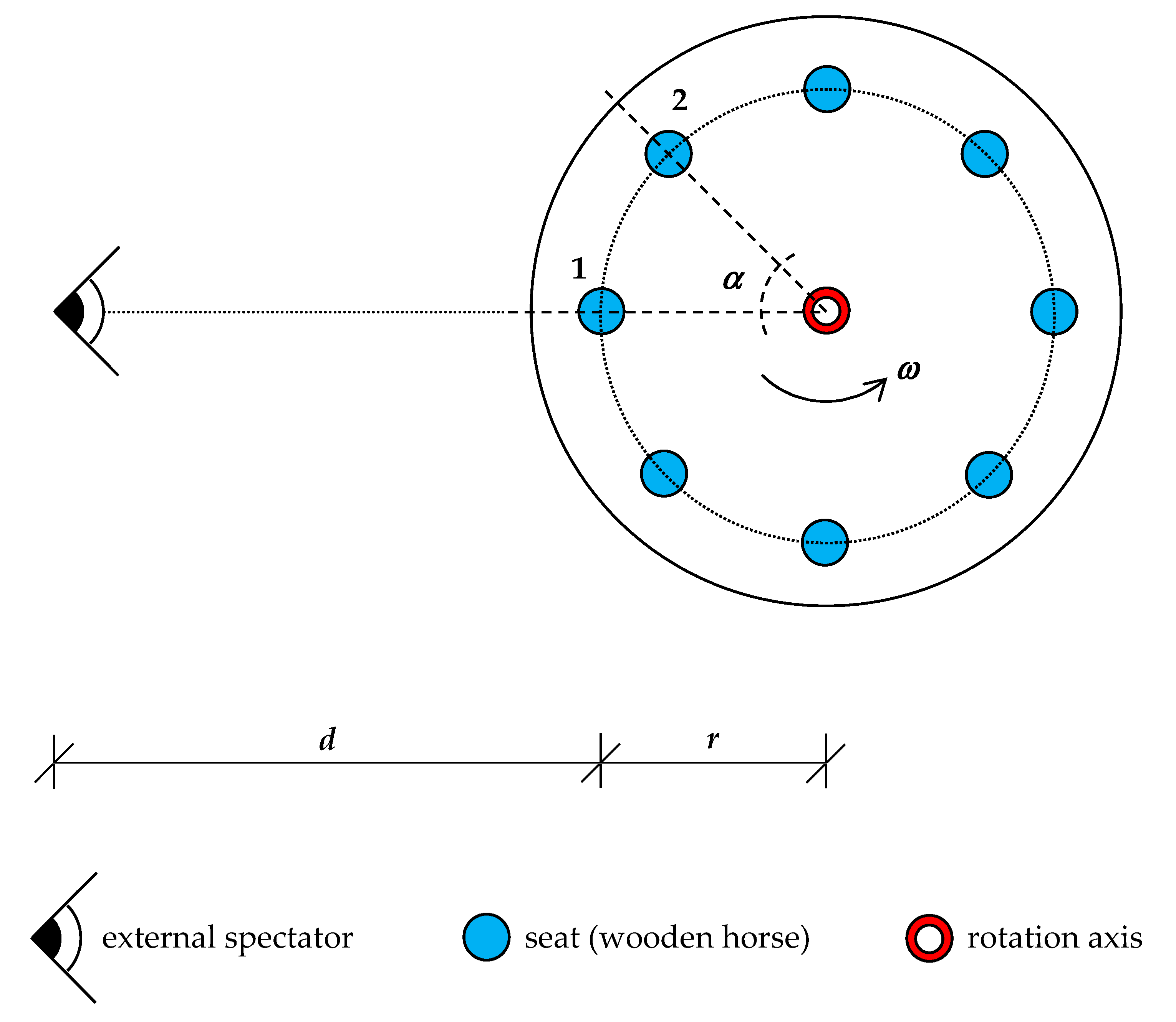
A frequency-based service may be described by adopting the Merry-Go-Round (MGR) paradigm: a roundabout (see Figure 1) is based on a rotating circular platform with seats for riders which are, traditionally, in the form of rows of wooden horses or other animals mounted on posts. However, a merry-go-round has the following property: “it shows each rider (i.e., wooden horse) to an external spectator at regular time intervals”.
Hence, in the case of uniform circular motion, let ω be the constant angular velocity of the merry-go-round around the rotation axis, and let r be the distance of each seat from the rotation axis. In this case, the tangential velocity of each seat, indicated as vseat, may be expressed as:
vseat = ω·r
Let Nseat be the number of the seats on the same row. With the assumption that the seats are equidistant along the same circumference, the angular distance between two successive seats, indicated as α, may be expressed as follows:
Likewise, the distance between two successive seats along the circular arc, indicated as dseat, may be expressed as:
dseat = α·r
Hence, with the above assumptions, the headway of the merry-go-round, indicated as HMGR, which represents the regular time interval for a seat to occupy the position of the previous seat (i.e., in the case of Figure 1, the time interval for an external spectator to see seat 2 in the position of seat 1), may be expressed as the ratio between Equations (1) and (3), that is:
Moreover, by substituting Equation (2) into Equation (4), we obtain:
It is worth noting that we may define the cycle time of a merry-go-round, indicated as CTMGR, as the time interval required by a seat (for instance seat 1 in Figure 1) to make a complete rotation and reach the initial configuration. In this case, the cycle time may be expressed as:
By combining Equation (5) with Equation (6), we obtain the following equation:
which represents the fundamental equation of the Merry-Go-Round (MGR) paradigm. In particular, HMGR and CTMGR being continuous quantities depending only on ω (see Equations (5) and (6)), once the number of seats Nseat has been fixed, for any value of HMGR, it is always possible to identify a corresponding value of CTMGR (or, equivalently, for any value of CTMGR, it is always possible to identify a corresponding value of HMGR) satisfying Equation (7).
HMGR·Nseat = CTMGR
However, Equation (7) is based on the following assumptions:
- all analyses are based on a regime condition (i.e., the transition phases are neglected) in the case of a uniform circular motion;
- all merry-go-round elements are rigidly tied to the rotating circular platform (i.e., the rotation axis, as well as the angular velocity, is unique for all elements);
- all seats (i.e., wooden horses) have the same dimensions and are equally spaced;
- all seats (i.e., wooden horses) are aligned on the same row (i.e., the tangential velocities are the same for all seats).
Obviously, in the case of seats aligned on different rows, it is necessary to apply the above equations for any row.
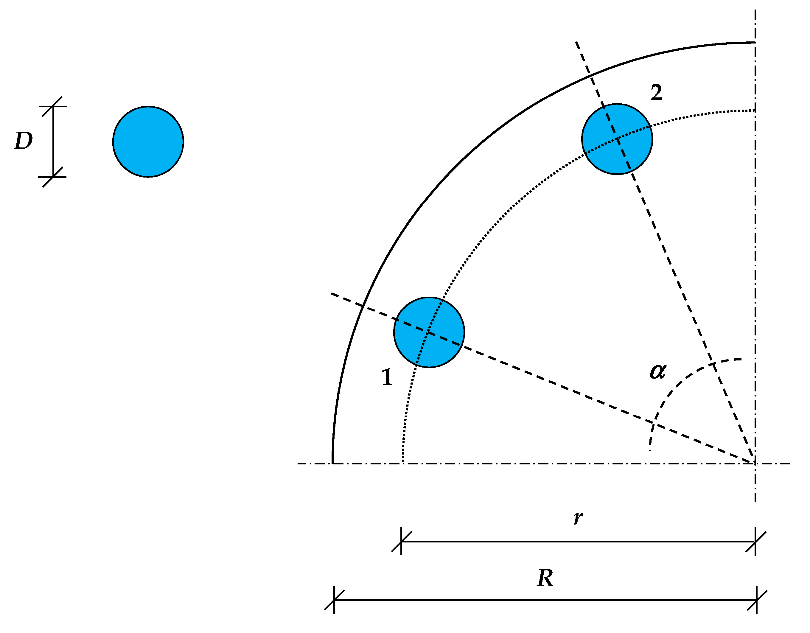
Moreover, since all the elements are rigidly tied to the rotating circular platform, it is necessary to impose some spatial constraints. With reference to Figure 2, let D be the maximum overall dimension of a seat (i.e., wooden horse). The distance between gravity centres of consecutive elements has to be no lower than D, that is:
α·r ≥ D
By substituting Equation (2) into Equation (8), we obtain the following constraint:
The second spatial constraint is based on the assumption that the circular platform is able to carry all seats. Hence, let R be the radius of the circular platform. It has to be no lower than r plus the semi-dimension of the seats, that is:
Obviously, all elements being rigidly tied to the circular platform, the above constraints (i.e., Equations (9) and (10)) are independent of the adopted motion regime. In the case of seats aligned on different rows, the above constraints have to be imposed for any row. Moreover, according to Equation (10), each row has to be considered as a circular platform for all inner rows.
However, the two spatial constraints show that, having fixed the dimensions of the circular platform (i.e., parameter R) and of the seats (i.e., parameter D), the number of seats (Nseat) and the radius of the row (i.e., parameter r) cannot be arbitrarily fixed.
In this context, as shown in Figure 3, if we consider passengers waiting on a station platform as external spectators of a roundabout and the rail convoys as the riders (i.e., wooden horses), we may analyse a rail service by adopting the Merry-Go-Round paradigm. Obviously, it is necessary to take into account the following differences:
- in a roundabout, the seats are rigidly tied to the rotating platform (i.e., there is no relative motion), while, in a railway context, the railway tracks are fixed (rigidly tied to the ground) and the rail convoys are in motion;
- in a roundabout, except for the transition phases (i.e., initial and final phases), all elements may be in a condition of (circular) uniform motion, while in a railway context, the rail convoys (the only non-fixed elements) reach a uniform condition only in some phases since: (a) they have to stop at stations to allow boarding/alighting of passengers; (b) they have to respect speed limits along the railway line;
- in a roundabout, all elements are spatially synchronised (i.e., being fixed to the platform, they keep their relative distances constant), while in a railway context, since the stations are not equidistant and the speed limits may vary along the line, even in uniform service conditions (i.e., all rail convoys have the same features in terms of priority, speed limits, and speed profiles), rail convoys may vary their relative distances continuously.
However, in a railway context, in the case of uniform service conditions, it is possible to guarantee the succession of trains so as to ensure constant time spacing (i.e., the Merry-Go-Round paradigm). Hence, it is necessary to analyse preliminarily the motion of an isolated rail convoy.
Since a rail convoy has to stop at stations in order for passengers to board/alight, it may assume at least three different motion conditions:
- an acceleration phase, where the train increases its speed (starting from a stop condition) up to the desired speed of the track section (generally, the minimum between the maximum speed of the considered train and the speed limit of the track section);
- a cruising phase, where the train travels at a constant speed;
- a braking phase, where the train reduces its speed (until it comes to a halt).
Obviously, in some cases (for instance when two successive stations are very close), the cruising phase may be absent since it is not possible to reach the desired speed during the acceleration phase and the braking phase is required in advance. Moreover, if different (desired) speeds are required in a track section between two successive stations, further motion phases have to be adopted (i.e., acceleration, cruising, braking phases) so as to respect the speed requirements. Finally, in some cases such as the case of energy-saving applications based on adopting proper driving speed profiles (for details, see [45]), a further motion phase may be adopted, indicated as a coasting phase, where the engine stops and the train moves by inertia.
In some cases, railway services are performed by means of two joint circular lines: a clockwise and an anticlockwise line. Although from a functional point of view, they can be considered joint services (i.e., a passenger chooses a line or its opposite according to his/her travel needs and uses the other line in his return journey), from an operational point of view, they may be considered independent services since frequencies, as well as rolling stock and driver shifts, can be set independently (i.e., it is possible to assign different service frequencies to the two lines or use different rolling stock). Hence, in the case of two joint circular lines, we may adopt the Merry-Go-Round paradigm by considering two independent lines (i.e., the following formulations have to be applied twice).
With the above definitions, it is possible to define the minimum cycle time of a rail convoy, indicated as , as the time interval required by a train to make a complete outward trip starting from the first terminus, carry out all the preparatory operations to undertake the return trip, starting from the second terminus, complete the return trip, and carry out all the preparatory operations to undertake the outward trip once again. Hence, the minimum cycle time may be calculated simply by adding all the times mentioned above, that is:
where rtlot and rtlrt are the running times between two successive stations associated, respectively, with links lot and lrt; lot and lrt are the generic track sections (i.e., links) associated, respectively, with the outward trip (ot) and return trip (rt); dtlot and dtlrt are the dwell times associated, respectively, with station platforms sot and srt; sot and srt are the generic station platforms associated, respectively, with the outward trip (ot) and return trip (rt); itot and itrt are the inversion times (i.e., the times spent in the preparatory operations to undertake the subsequent trip) associated, respectively, with the outward trip (ot) and return trip (rt).
Since the terms of Equation (11) have to be considered as realisations of random (i.e., stochastic) processes due to their variability, each term may be expressed as the sum of its mathematical expectation (i.e., the first moment or mean) and its random residual, as analysed in detail in Appendix A.1. In particular, represents the mathematical expectation of , that is:
where represents the random residual of the minimum cycle time.
Moreover, since a primary delay occurs when the real cycle time is higher than the planned one (i.e., a rail convoy arrives later than scheduled), in order to minimise delays, it is necessary to extend cycle time durations by adopting proper time extensions to offset time increases. In particular, having fixed a confidence level of and calculated the corresponding extension time (indicated as ), we may adopt a planned cycle time, indicated as , being calculated as follows:
such that the probability of the minimum cycle time being no higher than the planned one is equal to θ, that is:
By substituting Equations (12) and (13) into Equation (14), we obtain:
Hence, knowing the statistical distribution of , it is possible to determine the corresponding value of parameter which satisfies Equation (15). Details on the calculation of parameter can be found in [45].
Generally, term is split into two contributions: one associated with the outward trip (indicated as ) and one with the return trip (indicated as ), that is:
By extending the above analyses (i.e., Equations (11)–(16), as well as equations reported in Appendix A.1) in the case of multiple rail convoys (i.e., a real railway service), it is necessary to take into account that:
- the signalling system imposes a minimum distance (whose value may depend on the track section features) between two consecutive trains in order to avoid accidental collisions. Hence, a delayed train may affect the motion of a rail convoy in time;
- although a train can generally be overtaken at particular locations of a railway network (for instance, at stations), the assumption of the Merry-Go-Round paradigm imposes that the sequence of rail convoys has to be kept fixed.
The above aspects imply that there is a problem of delay propagation between consecutive rail convoys indicated in the literature as the secondary delay. In particular, in order to mitigate effects of secondary delays, the planned cycle time has to be modified by adding a further term, indicated as the buffer time, that is:
where is the scheduled cycle time; is the buffer time (i.e., the time extension of the planned cycle time) being calculated according to a confidence level equal to . Details on the calculation of term can be found in [46]. However, term is split into two contributions: that associated with the outward trip (indicated as ) and the one associated with the return trip (indicated as ), that is:
and Equation (17) may be expressed as:
Let HRAIL be the headway of the considered railway service (i.e., the time interval for a train to occupy the position of the previous train) and let Ntrain be the number of rail convoys to perform the service. In order to satisfy the Merry-Go-Round paradigm, according to Equation (7), it is possible to formulate the following equation:
However, since is fixed, representing the sum of physical times (i.e., running, dwell, and inversion) and times for recovery delays (depending only on confidence levels and ), the service headway HRAIL cannot be set arbitrarily since it has to respect Equation (20) jointly with the requirement that Ntrain has to be a positive integer number (i.e., ).
Hence, in order to avoid this limitation in feasible values of service headway, it is possible to consider an additional time, termed layover time, which represents the time spent by a train at the initial stations waiting for the departure time. In this context, if LT is the layover time, then it is possible to define the real cycle time, indicated as , as follows:
Additionally, in this case, term LT may be split into two contributions: that associated with the outward trip (namely ltot) and that for the return trip (ltrt), that is:
and Equation (21) may be expressed as:
By adopting term instead of term , we may reformulate Equation (20) as follows:
It is worth noting that this formulation allows us to overcome the above limitations. Indeed, in this case, for any desired value of HRAIL, it is always possible to identify a corresponding value of LT (or, equivalently, two values, ltot and ltrt) which allows Equation (24) (by affecting value) and the integer constraint of term Ntrain to be jointly satisfied. Hence, theoretically, we may consider a railway service with any value of headway, where, by combining Equations (21) and (24), we obtain:
It is worth noting that Equation (24) represents the fundamental equation proposed by [7] for describing a railway service analytically. Indeed, as mentioned above, the proposed approach, based on the Merry-Go-Round paradigm, provides the same results as the traditional approach by analysing the problem from a different perspective.
The constraints on rolling stock, that is, the minimum and the maximum number of trains required to perform a service, are analysed in Appendix A.2.
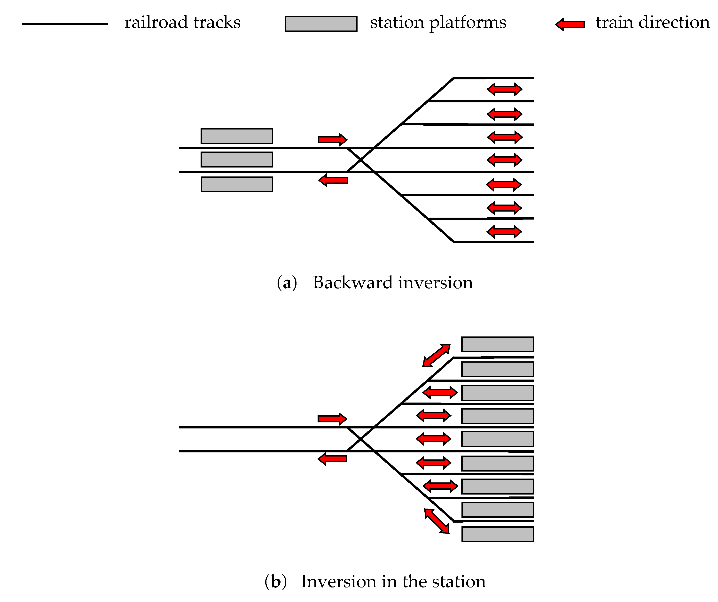
However, in order to analyse effects of terminal layouts on the implementation of the Merry-Go-Round paradigm, we have to consider two different configurations according to the relative position between the inversion tracks and the platform location (Figure 4): backward inversion and inversion in stations.
In the first case (i.e., Figure 4a), the train arrives in the station and, once all passengers have alighted, it leaves to reach the inversion area. Then, having completed all preparation phases (inversion, extension, and buffer times), the train reaches the station again where it waits for the passengers to board (i.e., the dwell time). In this case, the layover time can be spent on the inversion track or, equivalently, at the station platform.
Likewise, in the second case (i.e., Figure 4b), the train arrives in the station at the terminal track where it spends all times including the two dwell times (for alighting passengers when it arrives and for boarding passengers just before leaving) and the layover time.
In the case of the “backward inversion” configuration (i.e., Figure 4a), let , , and be, respectively, the inversion, extension, and buffer times associated with the i-th inversion track at the x-th terminal, where x may assume the value ot (i.e., in the case of the outward trip) or rt (i.e., in the case of the return trip). The corresponding layover time may be indicated as . In order to satisfy the MGR paradigm, all trains have to spend the same time regardless of the i-th track used, that is:
where , , , and are the general terms indicated in the Merry-Go-Round formulation (i.e., Equations (11)–(25)); Ix is the set of inversion tracks associated with the x-th terminal.
If we assume that the difference in variability among terms may be neglected, term does not depend on the i-th inversion track, such that:
However, if we want to consider difference in variability among terms , we have to fix the general term equal to the maximum among terms and apply this value to any inversion track. That is, Equation (26) has to be rewritten as:
with:
Likewise, since the buffer time has to be fixed to allow for interaction between successive rail convoys regardless of the inversion track used, it is independent of i, that is:
Equations (27) and (30) modify Equation (26) (or Equation (28)) into:
which expresses that:
- the higher the inversion time, the lower the layover time;
- or equivalently, the lower the inversion time, the higher the layover time.
Operatively, in order to determine the terms of Equation (31), once the inversion times are known for each track (i.e., term ), it is necessary to fix term as follows:
Then, by adopting Equation (A9), we may determine term ltx. Finally, term may be calculated by means of Equation (31) as follows:
The above formulation is based on the assumption that the time spacing between subsequent trains is kept constant along the entire line. This means that a rail convoy departs from the last station and reaches the switching point only after the previous train has left the switching point. Hence, a different number of inversion tracks in a station does not affect service performance.
However, by removing the above assumption (i.e., the use of constant time spacing) and adopting a swap technique between two successive trains (i.e., the rail convoys swap their function in terms of cycle time definition), we may increase the performance of the line. Indeed, we may assume that a rail convoy departs from the last station while the previous train is completing preparation phases at the inversion track, without waiting for it to leave the switching point. The previous train will depart once the subsequent train has arrived at the inversion track.
Although for a single train, all times (and related analytical formulations) analysed above remain constant, in terms of estimation of scheduled cycle time (i.e., term ), use of the swap technique allows the presence of buffer and extension times to be neglected, as well as the inversion time to be reduced to the mere contribution of running time on the inversion tracks. This means that:
- the lower the cycle time, the higher the service frequencies (or the lower the service headway) with the same number of rail convoys;
- or equivalently, the lower the cycle time, the lower the number of required rail convoys with the same service frequency (or service headway).
Obviously, in order to implement this improved scenario, at least two inversion tracks have to be available. However, the availability of additional tracks (i.e., a number greater than two) does not allow further improvements to the service performance.
A similar analysis may be implemented in the case of “inversion in the station” (i.e., Figure 4b). Indeed, since each train has to spend the same time regardless of the i-th track used, in this case, the MGR paradigm implies the following condition:
with:
where and are, respectively, the dwell time for alighting passengers when a train arrives at the i-th platform (i.e., the platform associated with the i-th inversion track) of the n-th station of the x-th trip and the dwell time for boarding passengers just before leaving from the i-th platform of the same station, which represents the first station of the subsequent trip (i.e., the y-th trip), and and are, respectively, terms and to be adopted in the general formulation of the Merry-Go-Round paradigm (i.e., Equations (11)–(25)).
Since the dwell time duration is related to the number of passengers wishing to alight or board, it does not depend on the inversion track used. Hence, we may assume:
Moreover, adopting for extension and buffer times considerations similar to those made in the case of “backward inversion” configuration, we may adopt Equations (27) and (30) (or, equivalently Equations (29) and (30)) also in the case of “inversion in the station”. Hence, Equation (34) may be changed to:
which, although it has formally the same formulation as Equation (31), may assume different values. Indeed, in this case (i.e., Figure 4b), the inversion time is evaluated from the switching point to the end of the inversion track used and from the end of the inversion track to the switching point. Differently, in the case of the “backward inversion” configuration (i.e., Figure 4a), the inversion time is evaluated from the platform of the last station to the end of the inversion track and from the end of the inversion track to the platform of the first station. It means that, in the case of “inversion in the station” layout, running times, which have to be computed up to the switching point, may be greater, while inversion times may be smaller with respect to the “backward inversion” configuration.
However, also in this case, a higher inversion time is associated with a lower layover time, or equivalently, a lower inversion time is associated with a higher layover time. Likewise, the terms of Equation (38) may be determined with a procedure similar to the case of “inversion in the station”. Indeed, once inversion times are known for each track (i.e., term ), we may calculate term according to Equation (32), term ltx by Equation (A9), and, finally, term by Equation (33).
In this case, the formulation concerning the time spacing among trains assumes that a rail convoy crosses the switching point only after the previous train has left the switching point. However, by removing this assumption and adopting a swap technique between two consecutive trains, we may assume that a rail convoy reaches the inversion track (i.e., the station platform) while the previous train is completing its preparation phase, and the waiting train will depart once the subsequent train has arrived. With this service framework (i.e., the adoption of a swap technique), in the cycle time definition, it is possible to neglect buffer and extension times, as well as the dwell times of the arriving and departing trains, besides reducing the inversion time only to the running time on the inversion tracks. Additionally, in this case, we may state that:
- the lower the cycle time, the higher the service frequencies (or the lower the service headway) with the same number of rail convoys;
- or equivalently, the lower the cycle time, the lower the number of required rail convoys with the same service frequency (or service headway).
However, this scenario may be implemented only if there are at least two inversion tracks where the availability of further additional tracks does not allow further improvements in the service.
4. Application to a Real Metro Line
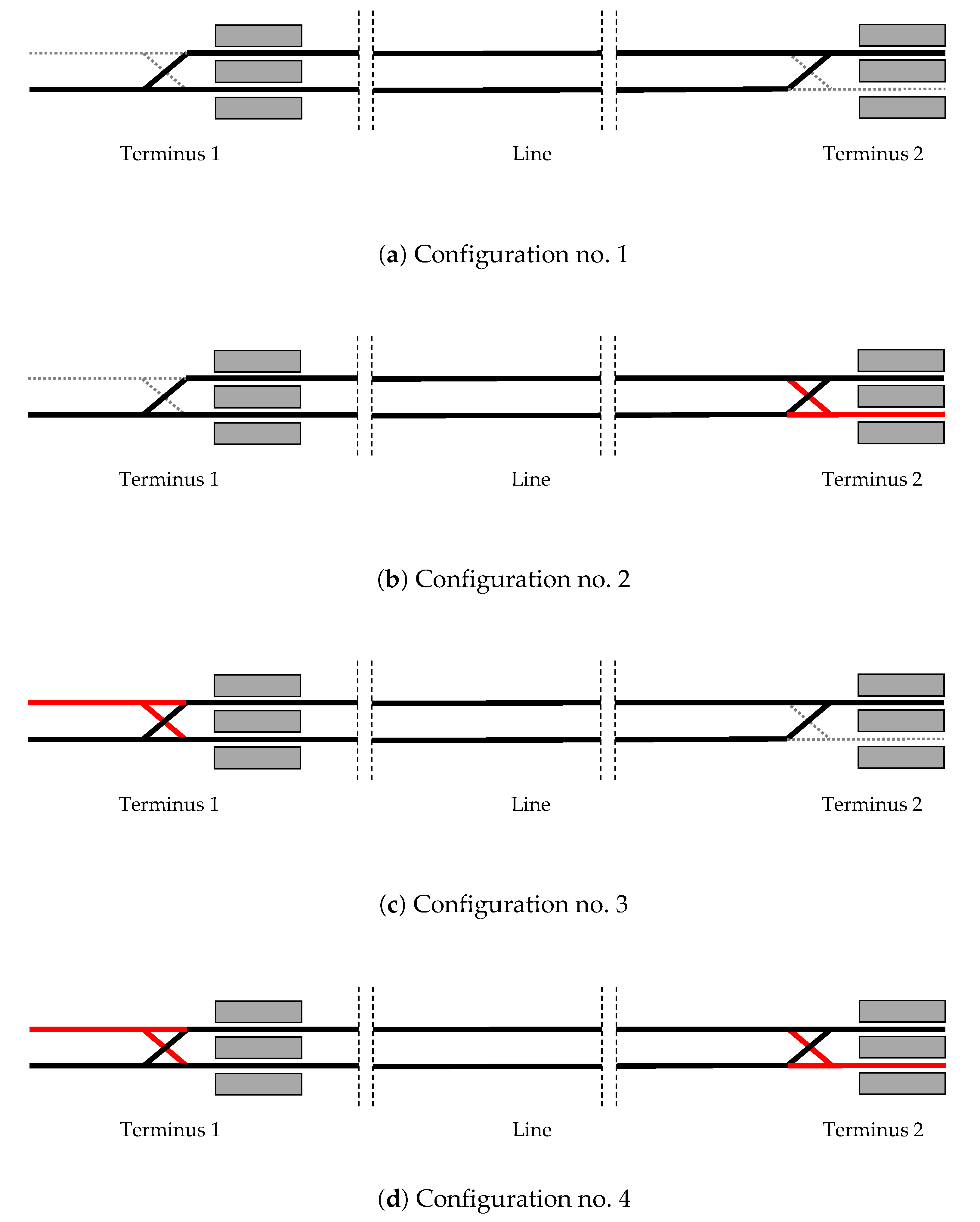
In order to show the feasibility and utility of the proposed approach, we applied it in the case of a real-scale railway line, where a frequency-based service is assumed. The main features of the line in question are reported in Figure 5. In particular, we considered a line with two terminals, each of them equipped with a single inversion track (Figure 5a—Configuration no. 1). The application consisted in analysing improvement effects due to the construction of an additional inversion track at the outward terminus (Figure 5b—Configuration no. 2), at the return terminus (Figure 5c—Configuration no. 3), or at both terminuses (Figure 5d—Configuration no. 4).
Table 1 provides service times for each analysed configuration. In particular, with a view to implementing some service improvements based on the adoption of a swap technique, we distinguished two contributions in the inversion time: train movement, which represents the time spent travelling from the switching points or the last station to the inversion track and vice versa, and train preparation, which is the time spent stationary on the inversion track where the train is prepared for the subsequent trip (change of cab, driver’s rest, cleaning operations, etc.). Moreover, in order to consider both feasible terminus layouts and related improvements, we assumed a “backward inversion” scheme in the first terminus of the outward trip and an “inversion in the station” scheme in the last terminus of the outward trip.
Data in Table 1 represents input data of the analytical formulations described in Section 3, which allows determining of railway service performance. In particular, in the case of Configuration 1 (i.e., both terminuses equipped with single inversion tracks), assuming a service headway of 7.50 min, from Equations (25) and (A13), it may be determined that the service requires at least 11 rail convoys and the related total layover time is 1.13 min. Moreover, by using Equation (24), it may be calculated that with a fleet of 11 trains, the minimum service headway is 7.40 min (i.e., a 1.37% reduction).
In the case of Configuration 2, which consists of adopting the improvements due to a second additional inversion track with a “backward inversion” scheme at the initial terminus of the outward trip (or, equivalently, at the final terminus of the return trip), jointly with the use of a swap technique between consecutive trains, we obtain the new times as shown in Table 1. In particular, times for train preparation, extension time, and buffer times associated with the return trip may be assumed as equal to zero. This implies an 8.42% reduction in scheduled cycle time. Hence, with a service headway of 7.50 min, from Equations (25) and (A13), it may be determined that the service requires at least 10 rail convoys (reduction of 9.09%) and the related total layover time is 0.48 min. Moreover, by adopting a fleet consisting of 10 trains, the minimum service headway calculated by means of (24) is 7.45 min. However, if we adopt the same number of rail convoys present in the unimproved condition (i.e., 11 rail convoys), we may obtain a minimum service headway of 6.77 min, which means a reduction of 9.68%.
In the case of Configuration 3, which consists of adopting the improvements due to a second additional inversion track with an “inversion in the station” scheme at the final terminus of the outward trip (or, equivalently, at the initial station of the return trip), jointly with the use of a swap technique between consecutive trains, we obtain the new times as shown in Table 1. Times for train preparation, extension time, and buffer times associated with the return trip may be assumed as equal to zero. Moreover, dwell times at the improved terminus may be assumed as equal to zero (only in terms of cycle time calculation) since a train departs when the next train arrives. These assumptions imply a 10.41% reduction in scheduled cycle time. Hence, with a service headway of 7.50 min, Equations (25) and (A13) may be used to determine that the service requires at least 10 rail convoys (9.09% reduction) and the related total layover time amounts to 2.10 min. Moreover, by adopting a fleet consisting of 10 trains, the minimum service headway calculated by means of (24) is 7.29. However, if we adopt the same number of rail convoys present in the unimproved condition (i.e., 11 rail convoys), we may obtain a minimum service headway of 6.63 min, which implies a reduction of 11.64%.
Finally, adopting the improvements due to a second additional inversion track at both terminuses (i.e., Configuration 4) and related swap techniques, we obtain the new times as shown in Table 1. In particular, by combining both improvements, we obtain an 18.82% reduction in scheduled cycle time. Hence, with a service headway of 7.50 min, Equations (25) and (A13) allow us to determine that the service requires at least nine rail convoys (reduction of 18.18%) and the related total layover time amounts to 1.45 min. Moreover, by adopting a fleet consisting of nine trains, the minimum service headway calculated by means of (24) is 7.34. However, if we adopt the same number of rail convoys present in the unimproved condition (i.e., 11 rail convoys), we may obtain a minimum service headway of 6.00 min, which means a reduction of 19.94%.
5. Conclusions and Research Prospects
In this paper, frequency-based systems were properly modelled by means of an analytical formalisation of the MGR paradigm. Indeed, just as a carousel has the property of showing wooden horses at regular time intervals to outside spectators, a frequency-based rail system has the property of showing trains at regular time intervals to the passengers waiting on the platform. It is worth noting that, to model the MGR effect accurately, it is necessary to take into account the role of the terminal station layout, which greatly affects system performance. This further aspect was thus extensively discussed and the whole framework was implemented in the case of a real-scale metro line.
The main findings concern the number of tracks required for the terminus stations. In order to comply with the MGR paradigm, only one inversion track for each terminus may be necessary. Moreover, service improvements may be achieved by adopting up to two inversion tracks per terminus.
It is worth noting that these results are valid in the case of isolated lines or terminuses devoted to single lines. Indeed, if the terminus station is shared by different lines, a maximum of two tracks per line are necessary for inversion tasks of convoys. Besides the coexistence of different lines, a number of tracks higher than that strictly required for the service may be useful for allowing recovery tasks. In other words, except where there is a depot in the middle of the line, which can feed both travel directions within the same time period, the need could arise for trains to queue on recovery tracks (other than those used for ordinary services) to avoid delays in operations. Indeed, if no recovery tracks are available, in the case of only one depot, a gap equivalent to the cycle time occurs in the service, while in the case of two depots serving the two terminal stations, this gap is equal to the maximum travel time between outward and return trips. Clearly, the greater the number of recovery tracks available, the lower the number of trains to be queued on a single track, thus allowing shorter tracks. Such observations confirm the significance of the proposed framework also in supporting design tasks related to the infrastructural layout.
Instead, in the case of more complex lines (e.g., lines with mixed freight and passenger traffic) or for managing unexpected events (e.g., service delays), the proposed theoretical framework could be embedded in a computer-aided decision support system, thus allowing simulation and forecasting tasks. Therefore, in regards to implications for future research, we propose applying the developed analytical framework in the case of different network contexts, as well as testing its effectiveness in supporting dispatching and rescheduling tasks such as implementation of energy-saving measures or the re-planning of rail services to cope with disruption.
Author Contributions
Conceptualization, L.D.; data curation, M.B.; formal analysis, L.D.; investigation, M.B. and L.D.; methodology, L.D.; validation, M.B. and L.D.; writing—original draft, M.B. and L.D.; writing—review and editing, M.B. and L.D. All authors have read and agreed to the published version of the manuscript.
Funding
This research was partially funded by Federico II University of Naples (Italy), grant number 000009-ALTRO-R-2020-LD “Department research DICEA”.
Institutional Review Board Statement
Not applicable.
Informed Consent Statement
Not applicable.
Data Availability Statement
The data used to support the findings of this study are available from the corresponding author upon request.
Conflicts of Interest
The authors declare no conflict of interest. The funders had no role in the design of the study; in the collection, analyses, or interpretation of data; in the writing of the manuscript, or in the decision to publish the results.
Appendix A
In this appendix, we propose two subsections where there are analysed in detail the stochastic analysis of the cycle time and the rolling stock constraints.
Appendix A.1. Stocastic Analysis of the Cycle Time
With the assumption that terms of Equation (11) have to be considered as the realisation of a random process due to their variability, each term may be expressed as the sum of its mathematical expectation and its random residual. Hence, assuming X is the generic element of Equation (11), the following may be expressed:
with:
where is the mathematical expectation of X; is the random residual of X; is the statistical distribution of ; is the vector of parameters describing the statistical distribution .
With the above assumptions, we may express Equation (11) as follows:
with:
and:
Appendix A.2. Rolling Stock Constraints
With the assumption of a fixed sequence of rail convoys (i.e., trains cannot be overtaken), layover times, as well as buffer times and time extensions, have to satisfy the following constraints:
By combining Equations (22) and (25), we obtain:
Likewise, by combining Equations (A7) and (A8), since the layover times have to be non-negative, we obtain:
Finally, by substituting Equation (A9) into Equation (A10), we obtain:
which, by means of (19), may be expressed as follows:
Therefore, since , we obtain the following constraints:
where and represent, respectively, the minimum and maximum number of trains required to perform the service.
References
- Caputo, A. Factors Affecting Atmospheric Emissions of CO2 and Other Greenhouse Gases within the Electricity Industry; Technical Report 257/2017; National Institute for Environmental Protection and Research (ISPRA): Rome, Italy, 2017. (In Italian) [Google Scholar]
- Canca, D.; Zarzo, A.; Algaba, E.; Barrena, E. Confrontation of Different Objectives in the determination of train scheduling. Procedia-Soc. Behav. Sci. 2011, 20, 302–312. [Google Scholar] [CrossRef] [Green Version]
- Canca, D.; Barrena, E.; Zarzo, A.; Ortega, F.A.; Algaba, E. Optimal Train Reallocation Strategies under Service Disruptions. Procedia-Soc. Behav. Sci. 2012, 54, 402–413. [Google Scholar] [CrossRef] [Green Version]
- Canca, D.; Zarzo, A. Design of energy-Efficient timetables in two-way railway rapid transit lines. Transp. Res. Part B Methodol. 2017, 102, 142–161. [Google Scholar] [CrossRef]
- Canca, D.; De-Los-Santos, A.; Laporte, G.; Mesa, J.A. The Railway Network Design, Line Planning and Capacity Problem: An Adaptive Large Neighborhood Search Metaheuristic. In Advances in Intelligent Systems and Computing; Springer: Cham, Switzerland, 2017; Volume 572, pp. 198–219. [Google Scholar]
- Ortega, F.A.; Mesa, J.A.; Piedra-De-La-Cuadra, R.; Pozo, M.A. A matheuristic for optimizing skip–stop operation strategies in rail transit lines. Int. J. Transp. Dev. Integr. 2019, 3, 306–316. [Google Scholar] [CrossRef] [Green Version]
- D’Acierno, L.; Botte, M.; Gallo, M.; Montella, B. Defining Reserve Times for Metro Systems: An Analytical Approach. J. Adv. Transp. 2018, 2018, 5983250. [Google Scholar] [CrossRef] [Green Version]
- Botte, M.; D’Acierno, L. Dispatching and Rescheduling Tasks and Their Interactions with Travel Demand and the Energy Domain: Models and Algorithms. Urban. Rail Transit. 2018, 4, 163–197. [Google Scholar] [CrossRef]
- D’Acierno, L.; Botte, M. Passengers’ Satisfaction in the Case of Energy-Saving Strategies: A Rail System Application. In Proceedings of the 2018 IEEE International Conference on Environment and Electrical Engineering and 2018 IEEE Industrial and Commercial Power Systems Europe (EEEIC/I&CPS Europe), Palermo, Italy, 12–15 June 2018; pp. 1–5. [Google Scholar]
- Kepaptsoglou, K.; Karlaftis, M. Transit Route Network Design Problem: Review. J. Transp. Eng. 2009, 135, 491–505. [Google Scholar] [CrossRef]
- Goossens, J.-W.; Van Hoesel, S.; Kroon, L. On solving multi-type railway line planning problems. Eur. J. Oper. Res. 2006, 168, 403–424. [Google Scholar] [CrossRef]
- Yu, B.; Yang, P.Z.; Yao, J. Genetic Algorithm for Bus Frequency Optimization. J. Transp. Eng. 2010, 136, 576–583. [Google Scholar] [CrossRef]
- Marín, A.; Jaramillo, P. Urban rapid transit network design: Accelerated Benders decomposition. Ann. Oper. Res. 2008, 169, 35–53. [Google Scholar] [CrossRef]
- Laporte, G.; Mesa, J.A.; Perea, F. A game theoretic framework for the robust railway transit network design problem. Transp. Res. Part B Methodol. 2010, 44, 447–459. [Google Scholar] [CrossRef]
- Fan, W.D.; Machemehl, R.B. Optimal Transit Route Network Design Problem with Variable Transit Demand: Genetic Algorithm Approach. J. Transp. Eng. 2006, 132, 40–51. [Google Scholar] [CrossRef]
- Marín, Á.; García-Ródenas, R. Location of infrastructure in urban railway networks. Comput. Oper. Res. 2009, 36, 1461–1477. [Google Scholar] [CrossRef]
- Gallo, M.; Montella, B.; D’Acierno, L. The transit network design problem with elastic demand and internalisation of external costs: An application to rail frequency optimisation. Transp. Res. Part C Emerg. Technol. 2011, 19, 1276–1305. [Google Scholar] [CrossRef]
- D’Acierno, L.; Gallo, M.; Montella, B. Application of metaheuristics to large-scale transportation problems. In International Conference on Large-Scale Scientific Computing; Lecture Notes in Computer Science; Springer: Berlin/Heidelberg, Germany, 2014; Volume 8353, pp. 215–222. [Google Scholar] [CrossRef]
- Fan, W.D.; Machemehl, R.B. Tabu Search Strategies for the Public Transportation Network Optimizations with Variable Transit Demand. Comput. Civ. Infrastruct. Eng. 2008, 23, 502–520. [Google Scholar] [CrossRef]
- Guihaire, V.; Hao, J.-K. Transit network design and scheduling: A global review. Transp. Res. Part A Policy Pract. 2008, 42, 1251–1273. [Google Scholar] [CrossRef] [Green Version]
- Crenca, D.; Malavasi, G.; Ricci, S. Dependence of railway lines carrying capacity by signalling systems and track geometry. In Proceedings of the 1st International Seminar on Railway Operations Modelling and Analysis, Delft, The Netherlands, 8–10 June 2005. [Google Scholar]
- Schwanhäusser, W. Die Bemessung der Pufferzeiten im Fahrplangefüge der Eisenbahn. Ph.D. Thesis, RWTH Aachen University, Aachen, Germany, 1974. [Google Scholar]
- Bonora, G.; Giuliani, L. Computational criteria for estimating capacity of railway lines. Ing. Ferrov. 1982, 37, 441–447. (In Italian) [Google Scholar]
- International Union of Railways (UIC). UIC Leaflet 405-1: Method to be Used for the Determination of the Capacity of Lines; UIC: Paris, France, 1983. [Google Scholar]
- Schultze, K.; Gast, I.; Schwanhäusser, W. Sls Plus—Einführung, Technical Report, Berlin, Germany, 2015. Available online: https://docplayer.org/46924828-E-i-n-f-ue-h-r-u-n-g-sls-plus-streckenleistungsfaehigkeit-simulation-fahrplankonstruktion-stand-14-dezember-2015.html (accessed on 1 February 2021).
- International Union of Railways (UIC). UIC Code 406: Capacity, 2nd ed.; UIC: Paris, France, 2013. [Google Scholar]
- Gonzalez, J.; Rodriguez, C.; Blanquer, J.; Mera, J.M.; Castellote, E.; Santos, R. Increase of metro line capacity by optimisation of track circuit length and location: In a distance to go system. J. Adv. Transp. 2010, 44, 53–71. [Google Scholar] [CrossRef]
- Prencipe, F.P.; Petrelli, M. Analytical methods and simulation approaches for determining the capacity of the Rome-Florence “Direttissima” line. Ing. Ferrov. 2018, 73, 599–633. [Google Scholar]
- Lindfeldt, A. Railway Capacity Analysis: Methods for Simulation and Evaluation of Timetables, Delays and Infrastructure. Ph.D. Thesis, KTH Royal Institute of Technology, Stockholm, Sweden, 2015. [Google Scholar]
- Galatola, M. Rail operation analysis–Consistency and quality indexes. Ing. Ferrov. 2004, 59, 649–655. (In Italian) [Google Scholar]
- Rete Ferroviaria Italiana—RFI (Italian National Railway Infrastructure Manager). Computation Methods for Railway Capacity; Technical Report; RFI: Rome, Italy, 2011. (In Italian) [Google Scholar]
- Potthoff, G. Verkerhrsstnomungslehre 1; Transpress VEB Verlag für Verkehrswesen: Berlin, Germany, 1963. [Google Scholar]
- Corazza, G.R.; Musso, A. Railway operations and rail stations. Long-term testing. Ing. Ferrov. 1991, 46, 607–618. (In Italian) [Google Scholar]
- Deutsche Bahn. Guidelines for Determining the Performance of Route Nodes; DB: Berlin, Germany, 1979. (In German) [Google Scholar]
- Malavasi, G.; Molková, T.; Ricci, S.; Rotoli, F. A synthetic approach to the evaluation of the carrying capacity of complex railway nodes. J. Rail Transp. Plan. Manag. 2014, 4, 28–42. [Google Scholar] [CrossRef]
- Nuzzolo, A.; Russo, F.; Crisalli, U. A Doubly Dynamic Schedule-based Assignment Model for Transit Networks. Transp. Sci. 2001, 35, 268–285. [Google Scholar] [CrossRef]
- Hamdouch, Y.; Lawphongpanich, S. Schedule-based transit assignment model with travel strategies and capacity constraints. Transp. Res. Part B Methodol. 2008, 42, 663–684. [Google Scholar] [CrossRef]
- Hamdouch, Y.; Ho, H.; Sumalee, A.; Wang, G. Schedule-based transit assignment model with vehicle capacity and seat availability. Transp. Res. Part B Methodol. 2011, 45, 1805–1830. [Google Scholar] [CrossRef]
- Hamdouch, Y.; Szeto, W.; Jiang, Y. A new schedule-based transit assignment model with travel strategies and supply uncertainties. Transp. Res. Part B Methodol. 2014, 67, 35–67. [Google Scholar] [CrossRef] [Green Version]
- Ercolani, M. The use of microsimulation models for the planning and management of metro systems. WIT Trans. Built Environ. 2014, 135, 509–521. [Google Scholar] [CrossRef] [Green Version]
- Nguyen, S.; Pallottino, S.; Gendreau, M. Implicit Enumeration of Hyperpaths in a Logit Model for Transit Networks. Transp. Sci. 1998, 32, 54–64. [Google Scholar] [CrossRef]
- Wong, S.C.; Yang, C.; Lo, H.K. A path-based traffic assignment algorithm based on the TRANSYT traffic model. Transp. Res. Part B Methodol. 2001, 35, 163–181. [Google Scholar] [CrossRef]
- Maadi, S.; Schmöcker, J.-D. Optimal hyperpaths with non-additive link costs. Transp. Res. Part B Methodol. 2017, 105, 235–248. [Google Scholar] [CrossRef]
- D’Acierno, L.; Botte, M.; Montella, B. Assumptions and simulation of passenger behaviour on rail platforms. Int. J. Transp. Dev. Integr. 2018, 2, 123–135. [Google Scholar] [CrossRef] [Green Version]
- D’Acierno, L.; Botte, M. A Passenger-Oriented Optimization Model for Implementing Energy-Saving Strategies in Railway Contexts. Energies 2018, 11, 2946. [Google Scholar] [CrossRef] [Green Version]
- International Union of Railways (UIC). UIC CODE 451-1: Timetable Recovery Margins to Guarantee Timekeeping—Recovery Margins; UIC: Paris, France, 2000. [Google Scholar]
Figure 1.
Elements of a merry-go-round.

Figure 2.
Seat details in a merry-go-round context.

Figure 3.
Comparison between a merry-go-round and a railway line.

Figure 4.
Terminal layout configurations.

Figure 5.
Terminal layout configurations.

Figure 6.
Service times in the case of outward trip.

Figure 7.
Service times in the case of return trip.

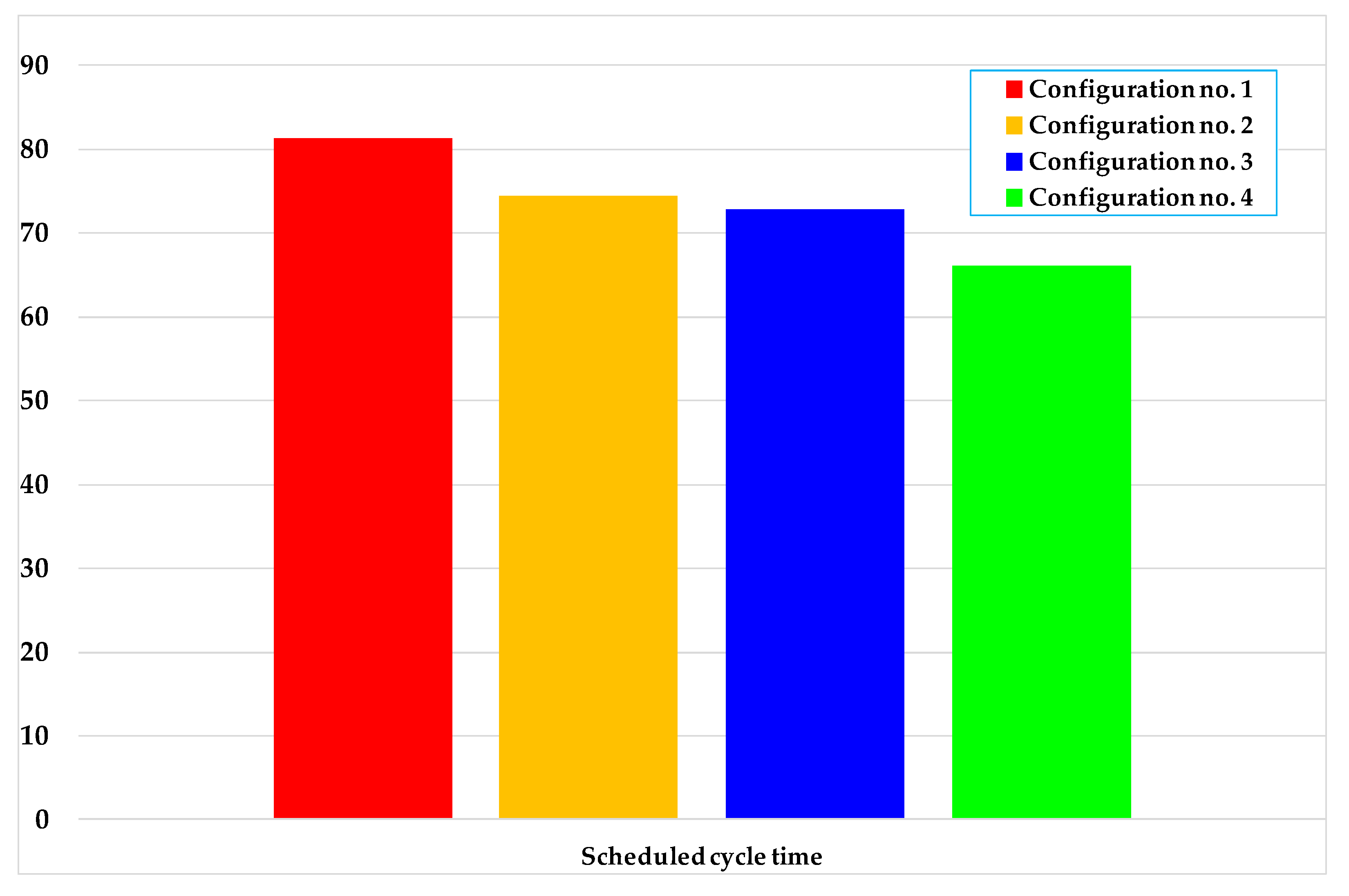
Figure 8.
Scheduled cycle times.


Table 1.
Service times in the case of different terminal layout configurations.
| Configuration No. 1 | Configuration No. 2 | Configuration No. 3 | Configuration No. 4 | ||||||
|---|---|---|---|---|---|---|---|---|---|
| Outward Trip (min) | Return Trip (min) | Outward Trip (min) | Return Trip (min) | Outward Trip (min) | Return Trip (min) | Outward Trip (min) | Return Trip (min) | ||
| Total running time | 24.37 | 24.77 | 24.37 | 24.77 | 24.37 | 24.77 | 24.37 | 24.77 | |
| Total dwell time | 7.33 | 7.33 | 7.33 | 7.33 | 6.00 | 7.33 | 6.00 | 7.33 | |
| Inversion time | Train movement | 2.12 | 1.47 | 2.12 | 1.47 | 2.12 | 1.47 | 2.12 | 1.47 |
| Train preparation | 3.00 | 3.00 | 3.00 | 0.00 | 0.00 | 3.00 | 0.00 | 0.00 | |
| Extension time | 2.18 | 1.93 | 2.18 | 0.00 | 0.00 | 1.93 | 0.00 | 0.00 | |
| Buffer time | 1.95 | 1.92 | 1.95 | 0.00 | 0.00 | 1.92 | 0.00 | 0.00 | |
| Total | 40.95 | 40.42 | 40.95 | 33.57 | 32.48 | 40.42 | 32.48 | 33.57 | |
| Scheduled cycle time | 81.37 | 74.52 | 72.90 | 66.05 | |||||
Publisher’s Note: MDPI stays neutral with regard to jurisdictional claims in published maps and institutional affiliations. |
© 2021 by the authors. Licensee MDPI, Basel, Switzerland. This article is an open access article distributed under the terms and conditions of the Creative Commons Attribution (CC BY) license (http://creativecommons.org/licenses/by/4.0/).
Share and Cite
MDPI and ACS Style
D’Acierno, L.; Botte, M. Railway System Design by Adopting the Merry-Go-Round (MGR) Paradigm. Sustainability 2021, 13, 2033. https://0-doi-org.brum.beds.ac.uk/10.3390/su13042033
AMA Style
D’Acierno L, Botte M. Railway System Design by Adopting the Merry-Go-Round (MGR) Paradigm. Sustainability. 2021; 13(4):2033. https://0-doi-org.brum.beds.ac.uk/10.3390/su13042033
Chicago/Turabian StyleD’Acierno, Luca, and Marilisa Botte. 2021. "Railway System Design by Adopting the Merry-Go-Round (MGR) Paradigm" Sustainability 13, no. 4: 2033. https://0-doi-org.brum.beds.ac.uk/10.3390/su13042033
Note that from the first issue of 2016, this journal uses article numbers instead of page numbers. See further details here.