
The Dynamic Correlation among Financial Leverage, House Price, and Consumer Expenditure in China


1
Business School of Nanjing, Xiaozhuang University, Nanjing 211171, China
2
Department of Information Management, Chang Gung University, Taoyuan 33302, Taiwan
3
Clinical Trial Center, Chang Gung Memorial Hospital, Taoyuan 33305, Taiwan
4
Department of Industrial Engineering and Management, Ming Chi University of Technology, New Taipei City 24301, Taiwan
5
Department of Agriculture and Applied Economics, University of Georgia, Athens, GA 30602, USA
6
Business School, Jinling Institute of Technology, Nanjing 211169, China
*
Author to whom correspondence should be addressed.
Sustainability 2021, 13(5), 2617; https://0-doi-org.brum.beds.ac.uk/10.3390/su13052617
Submission received: 27 January 2021
/
Revised: 23 February 2021
/
Accepted: 24 February 2021
/
Published: 1 March 2021
Abstract
:With the help of the time-varying parameter vector autoregression with stochastic volatility (TVP-SV-VAR) model and the Bayesian dynamic conditional correlational autoregressive conditional heteroscedasticity (Bayesian DCC-GARCH) model, this study analyzes the interaction mechanism and dynamic correlation among financial leverage, house price, and consumer expenditure (the survey data are collected from China’s National Bureau of Statistics from January 2000 to December 2019; the data on financial leverage and consumer expenditure are from the Wind economic database, and the price of commercial housing was calculated based on the sales volume and area of commercial housing on the official website of China’s National Bureau of Statistics). Empirical results show that an increase in financial leverage significantly increases house prices and reduces consumer expenditure, that a rise in house prices inhibits financial leverage and weakens consumer expenditure, and that an increase in consumer expenditure raises financial leverage and stimulates a rise in house prices. In addition, house price and consumer expenditure are most relevant, followed by financial leverage and consumer expenditure, and then by financial leverage and house price. Therefore, systematic analysis of dynamic correlation among the three variables has important practical significance for formulating appropriate financial policies to stabilize house prices and promote the growth of consumer expenditures. Specially, financial leverage is an important factor to hold back soaring house prices and shrinking consumer expenditure. Therefore, monetary and macroprudential policies should be used to deal with financial leverage variables in order to achieve a balanced and sustainable development of the macroeconomy in China.
1. Introduction
After more than 40 years of rapid development, China has achieved world-renowned economic growth but has accumulated more and more urgent problems to be resolved, such as a widening gap between the rich and the poor, lack of social security, and rising labor costs. Currently, problems like rising debt leverage, scarce land resources, and diminishing investment returns are increasingly constraining the development of China’s extensive economy. Chinese scholars are more and more aware that the economic growth mode driven solely by investment and foreign trade is no longer sustainable [1] In addition, the spread of anti-globalization, the rise of trade protectionism, China–US trade disputes, and the COVID-19 epidemic have exacerbated the deterioration of China’s foreign trade environment. Therefore, it is necessary to change its current mode of economic growth by transforming it from an extensive economy to an intensive economy and from being driven by investment and trade to being driven by consumption. Consumption is an inevitable factor to fundamentally expand the scale of production. A strong consumer demand can expand the scale of production and provide impetus for sustainable economic growth. Besides, consumption is closely related to not only an improvement in residents’ living standards but also the transformation and upgrading of the industrial structure. Therefore, how to effectively stimulate residents’ demand for consumption is increasingly becoming the key to transforming China’s economic growth mode and strengthening its sustainable economic growth (some opinions on improving the system and mechanism of promoting consumption and further stimulating the consumption potential of residents were issued by the Chinese government in 2018).
In recent years, the rapid rise in China’s financial leverage and house prices and the sharp decline in consumption growth have been striking. To avoid a hard landing of the economy due to the global financial crisis, the Chinese government implemented a “CNY four trillion” fiscal stimulus policy beginning from late 2008, local governments launched many supporting stimulus policies, and the People’s Bank of China reduced interest rates and deposit reserve ratios multiple times to inject sufficient liquidity into the market. As a result, the debt ratio of the government, enterprises, and even residents climbed up. Economic downturn has further caused the deterioration of the total social asset and resulted in continuous increases in the overall financial leverage of the society. China’s current financial leverage ratio (private sector credit/GDP) has far exceeded the average levels of the world’s major economies (groups), such as emerging economies, developed countries, and G20 countries, being second only to that of the United States and Japan. Its financial leverage also rose rapidly after 2008. However, the marginal utility of financial leverage has gradually declined. Especially during the current economic transformation, the real economy has generally low returns. Large amounts of credit funds have been allowed to idle for arbitrage among financial institutions, financial systems, and capital markets, which easily leads to the rapid accumulation of financial risks and a substantial decline in the stability of the finance sector. The most obvious signal in this regard is the huge volatility in the stock and bond markets recently (from 15 June to 9 July 2015, China’s A-share market plunged from 5178 points to 3373 points. In 2016, the prices of black futures, represented by rebar, iron ore, and coking coal, fluctuated sharply). The Chinese government noticed the seriousness of this problem; so it implemented a deleveraging strategy in 2015 and proposed to “improve monetary policy and macroprudential policy” and “control the main valve of money supply” in 2017 to strictly control the amount of money supply. Since then, credit growth has gradually declined and rise in financial leverage has slowed down.
Against the background of slowed macroeconomic growth and declining corporate profitability, house prices still remain high. Since the implementation of the housing system reform in 1998, house prices have risen sharply and rapidly in most of the years. In 2019, their cumulative increase exceeded 360%. (The data come from the official website of the National Bureau of Statistics of China. The housing price is the national average price). As the expected return on the real estate market is significantly higher than that on other assets or investments, a large part of credits went to the real estate market through various channels. A large number of high-risk, high-yield bonds are closely related to the real estate market and house prices. China’s current real estate market is closely related to the financial system and the macroeconomy. Great volatility in house prices will exert a huge impact on the stability of the financial system and the macroeconomy. Some studies have shown that the rapid increase in house prices and great volatility in the macroeconomy are closely related to financial leverage. A rapid increase in financial leverage is usually considered an early warning of potential risks. Excessive expansion of credit often leads to skyrocketing asset prices, increased external imbalances, and overheated economic operations, which in turn endanger the healthy operation of the entire financial system and the macroeconomy [2,3].
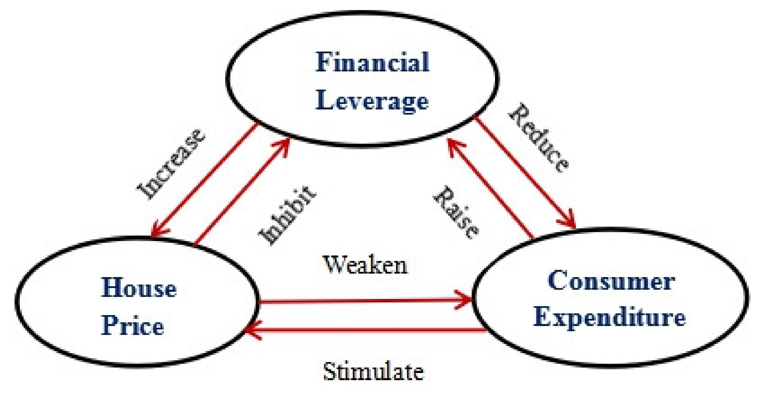
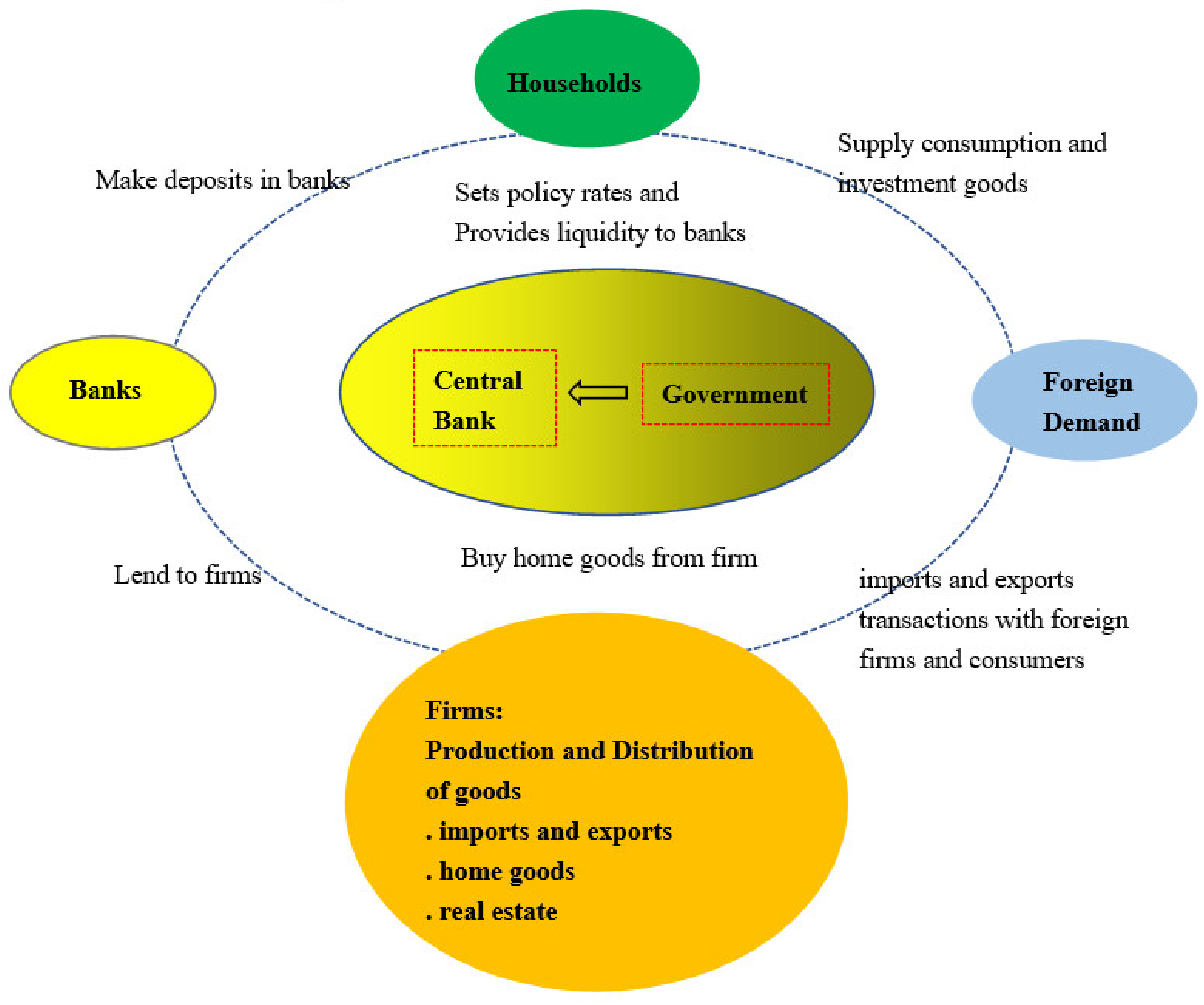
In stark contrast to continuous rises in financial leverage and house prices, consumer expenditure is sluggish. Data from the National Bureau of Statistics of China show that Chinese residents’ consumption rate from 2000 to 2010 declined from 46.7% to 35.6% and rebounded after 2010. China’s current consumption rate is not only significantly lower than that of major European and American economies but also lower than that of Japan and South Korea. According to the World Bank, its average consumption rate from 2016 to 2018 was 53.6%, being lower than that in the US (82.4%), in the UK (84.0%), in Germany (72.2%), in Japan (75.4%), and in South Korea (64.0%). What is even more disturbing is that the growth momentum of China’s consumption has been significantly weakened since 2017. The contribution rate of the final consumption spending to GDP growth has fallen from 66.5% in 2016 to 58.8% in 2019. The growth rate of total retail sales of consumer goods reached the lowest in 14 years, being only 10.2%, which further dropped to 9.4% in the first half of 2018. Figure 1 shows the relationship among China’s major macroeconomic sectors [4], indicating that financial leverage, house price, and consumer expenditure are closely related.
It is not difficult to see that in-depth analysis of the relationship among financial leverage, house price, and consumer expenditure can help us understand and resolve some important issues that China is facing (e.g., stabilizing leverage, stabilizing house price, and boosting consumption) and achieve sustainable economic growth. The main contents of the remaining parts of this article include the following: A literature review is in Section 2, which systematically sorts out and summarizes related literature. Theoretical analysis and model description are in Section 3. The interpretation of empirical results is in Section 4, which mainly includes analysis of the degree of mutual influence among financial leverage, house price, and consumer expenditure; the mechanism of action; and the dynamic correlation coefficient. Conclusions and recommendations are in Section 5.
2. Literature Review
Existing research on the relationship among financial leverage, house price, and consumer expenditure can be roughly divided into three categories: research on the impact of financial leverage on house price, research on the impact of financial leverage on consumer expenditure, and research on the impact of house price on consumer expenditure. Status quo and trends of domestic and foreign research in this regard are as follows:
2.1. The Impact of Financial Leverage on House Price
Regarding the impact of financial leverage on house price, Bernanke and Gertler (1989), Bernanke, Gertler, and Gilchrist (1999), and Gertler and Karadi (2011) introduced agency problem in financing contract to analyze how the financial market affects the macroeconomy via asset price. They believed that when the finance sector becomes more developed, the financial market or financial intermediaries will significantly amplify macroeconomic volatility through changes in asset price [5,6,7]. Herring and Wachter (1999) and Krugman (1999) held that excessive leverage of financial system is the main reason for bubbles in housing price [8,9]. Edelstein and Paul (2000) pointed out that the main reasons for real estate bubbles in Japan are an excessively low credit interest rate and excessive financial support caused by international capital flows [10]. Studies by Schularick and Taylor (2012), Carlin and Soskice (2012), and Geanakoplos and Zame (2014) revealed that the growth of the financial leverage ratio (private sector credit/GDP) is a key factor that drives rapid increases in asset price (including house price) [11,12,13]. Punzi (2013) and Gete and Reher (2016) conducted research with the DSGE (Dynamic Stochastic General Equilibrium) model and found that in countries with a developed financial market, house price is more sensitive to financial variables and that changes in house price significantly amplify macroeconomic volatility through the “financial accelerator” mechanism of lending among households) [14,15].
2.2. The Impact of Financial Leverage on Consumer Expenditure
As for the impact of financial leverage on consumer expenditure, Mishkin (1976) pointed out that there is a distinct negative correlation between consumption expenditure of households and the bank credit obtained by them [16]. Research by Bacchetta and Gerlach (1997) showed that there is a positive correlation among consumer credit, mortgage loans, and consumer expenditure [17], which is particularly obvious in the consumption of durable goods. Dynan et al. (2012) analyzed the Panel Study of Income Dynamics (PSID) and found that after the outbreak of the financial crisis in 2008, high-leverage households were forced to deleverage, which inhibited their consumption and delayed the recovery of the macroeconomy [18]. Dynan and Edelberg (2013) pointed out that excessive leverage weakens residents’ access to consumer credit support, thereby limiting their consumption expenditures and ultimately negatively affecting consumption and production [19]. Johnson and Li (2007) analyzed relevant data from 1992 to 2005 in the US and found that in the face of the same income changes, changes in consumption of high-leverage households far exceed those of low-leverage households [20]. Baker (2015) studied relevant data from 2008 to 2013 and found that when faced with the same income shock, high-leverage households showed a range of spending adjustment significantly greater than that of low-leverage households [21]. Mian et al. (2013) and Yao et al. (2015) analyzed relevant data from the US and Norway, respectively, and further proved that when facing the same increase in wealth, high-leverage households tend to increase consumption expenditure more than low-leverage households [22,23].
2.3. The Impact of House Price on Consumer Expenditure
Concerning the impact of house price on consumer expenditure, Case et al. (2005) conducted empirical research on data of many countries and found that the effect of wealth on the housing market is very obvious, that increase in house price can promote the increase of consumer expenditure, and that the effect of wealth on the stock market is very weak [24]. Carroll et al. (2006) employed the sluggishness of the consumption growth model and found there is a wealth effect on both short-term and long-term house price and that a rise in house price promotes an increase in consumer expenditure [25]. Mian and Sufi (2009) studied the relationship between house price and household borrowing and consumption with relevant US data from 1997 to 2008 and found rising house prices increase household borrowing, which is not used to repay loans but to buy consumables and decorate the house [26]. Bonis and Silvestrini (2012) pointed out that in OECD (Organization for Economic Co-operation and Development) countries, rising house prices have a very significant positive impact on consumption [27]. Cristini and Sevilla (2014) re-estimated the wealth effect of rising house price by setting a single model that incorporates the characteristics of multiple influence mechanisms and found that house price affects household consumption either through wealth effect or through common causality [28]. Catte et al. (2004) pointed out that house price exerts quite different influences on household consumption in different countries and regions. To be specific, countries such as Australia and the US face greater wealth effect, while in Germany and France, real estate has no significant impact on consumption [29]. Campbell et al. (2007) and Chanmon and Prasad (2010) believed that a rise in house prices causes some residents to save for house purchase, which increases residents’ saving rates and reduces their consumption [30,31].
In summary, the correlation among financial leverage, house price, and consumer expenditure has attracted more and more attention from scholars and the business community, but existing literature mainly focuses on the impact of financial leverage on house price. Researchers have not drawn a conclusion about the impact of financial leverage on consumer expenditure and the impact of house price on consumer expenditure. In addition, existing studies do not put financial leverage, house price, and consumer expenditure into the same framework to analyze their mutual influence or discuss the dynamic relationship among them. Therefore, this study makes two marginal contributions. First, existing empirical analyses lack discussion on time variants. With the passage of time, economic structure and other factors continue to change, so parameters of the econometric model should be changed accordingly. Traditional measurement models used in most existing studies cannot describe this dynamic feature, which has inevitably greatly compromised the accuracy of their conclusions. Therefore, this study chooses a dynamic measurement model for empirical analysis. Second, financial leverage, house price, and consumer expenditure are put into the same framework to systematically analyze the degree of mutual influence and dynamic correlation among them. Most existing studies focus on the degree of influence of financial leverage on house price, the degree of influence of financial leverage on consumer expenditure, and the degree of influence of house price on consumer expenditure in a unidirectional manner but ignore the mutual influence among them. This study systematically analyzes the interaction and dynamic correlation among financial leverage, house price, and consumer expenditure based on the time-varying parameter vector autoregression with stochastic volatility (TVP-SV-VAR) model and the Bayesian dynamic conditional correlational autoregressive conditional heteroscedasticity (Bayesian DCC-GARCH) model and makes policy recommendations on how to maintain a balanced and stable macroeconomic development, which makes it a useful supplement and expansion of existing research.
3. Theoretical Analysis and Model Description
3.1. Theoretical Analysis
The theory of financial deepening shows that excessive government intervention in financial activities obstructs the development of the financial system. Then the underdevelopment of the financial system will seriously hinder economic development, resulting in a vicious circle of financial repression and economic backwardness. On the contrary, developing countries can build a virtuous circle of financial reform and economic development through financial deepening (McKinnon, 1973; Shaw, 1973) [32,33]. Therefore, some studies believe that financial leverage can help push up house prices and stimulate consumer expenditure. Lambertini et al. (2013) confirmed a positive effect of short-term financial leverage on a country’s consumption level [34]. Gao et al. (2020), using China Family Panel Studies (CFPS) microdata, showed that increasing financial leverage in the short term can help stimulate household consumption expenditure [35]. By the life cycle model, Ruan et al. (2020) showed house prices are closely related to the leverage ratio of the residential sector and there is a significant self-reinforcing effect between them, which will magnify the impact on major macroeconomic variables, such as consumption and investment [36]. Ma and Zubairy (2020) claimed that due to the mechanism of collateral constraint, financial leverage will exert a non-negligible impact on consumption, investment, and total social output by acting on collateral prices (mainly house prices and stock prices) [37].
The debt deflation theory believes that a rise in financial leverage hinders economic growth, especially when debt accumulates to a certain extent, possibly causing the economy to fall into a circle of debt deflation, triggering a comprehensive and long-term economic recession. Once too much debt accumulates, facing more tightened constraints, companies and households have to reduce investment and consumption and sell assets at low prices to repay the debts due. This leads to a loss of net assets, a rapid decline in prices, and a rise in the level of real debt. Then, the circle of high level of debt and deflation ultimately exacerbates the economic recession (Fisher, 1933; Tobin, 1975) [38,39]. Therefore, some scholars believe that financial leverage will push up house prices but will shrink the consumer expenditure. Dynan et al. (2012) found that after the financial crisis, highly leveraged households were forced to reduce their consumptions. This high financial leverage inhibited aggregate demand and delayed the recovery of the economy. The reason is that after the financial crisis, highly leveraged households had to choose to deleverage. The reduction in household wealth inhibited consumer expenditure, and financial leverage played the role of an accelerator [18]. Mian et al. (2017), using cross-country unbalanced panel data, have shown that if the financial leverage ratio has a continuous upward trend, the consumption and output decrease significantly [40]. Scholnick (2013) claimed that a rapid rise in house prices caused by financial leverage makes households delay their consumption, which leads to a decline in consumer expenditure [41]. Mendoza (2010) found that the leverage ratio of the representative household with credit constraints rises rapidly during the period of economic expansion. When the leverage ratio is high enough, it triggers the constraint effect, which reduces the amount of credit and asset prices through a deflationary mechanism and finally affects consumption [42].
Based on permanent income hypothesis and life cycle hypothesis, the size of wealth and changes in wealth affect consumer expenditure (Friedman, 1957; Ando & Modigliani, 1963) [43,44]. Households can smoothly allocate their assets to consumption in each period. Therefore, a higher level of household assets leads to a higher level of consumption. Based on the life cycle-permanent income hypothesis, some studies have analyzed the effect of house price on financial leverage. Veirman and Duncan (2010) used New Zealand’s macrodata to show that most changes in real estate wealth and financial wealth are permanent changes, which have a lagging effect on consumption [45]. Burrows (2018) and Cloyne et al. (2019) showed that rising house prices increase the market value of real estate and families with a house can obtain more low-cost credit and release liquidity constraints. Therefore, they are able to maintain smooth consumption in each period [46,47]. China’s “house slave effect” is particularly obvious at this stage [48]. In the context of rapidly rising house prices, Chinese families often choose to cut down on spending on food and clothing, reduce consumption, and save for buying a house. Bernanke et al. (1996) found that the increase in the price of a house increases the value of the real estate as collateral, which improves the family’s borrowing capacity and pushes up the level of financial leverage [49]. Oikarinen (2009) and DeFusco (2018) found that rising housing prices increase the expected wealth of households, leading to more consumption and ultimately expanding credit demand. Due to the rise in house prices, it is common for a Chinese family to buy a house with a loan [50,51]. Higher house prices naturally lead to an increase in housing loans. The expectation of rising house prices also prompts families with housing demand to buy houses earlier with loans instead of renting [52].
Life cycle hypothesis and liquidity constraint theory are the main theoretical basis for analyzing the impact of consumer expenditure on financial leverage and house prices. Under the budget constraint, consumers allocate current consumption according to all expected income to maximize their utilities with smooth consumption using credit. The existence of liquidity constraints makes the impact of current income on consumption greater than that under the life cycle theory, and at the same time, consumers’ liabilities will be less than that under the life cycle theory. Stiglitz (2009) claimed that facing a stagnant wage income, poor households tend to use credit to maintain their living standards, thereby pushing up debt leverage [53]. Barba and Pivetti (2009) analyzed the reasons for the increase in household debt and found that income inequality and the desire to improve living standards are likely to lead to an increase in financial leverage [54].
Based on the above analysis, our study proposes two hypotheses:
Hypothesis 1.
Financial leverage, house prices, and consumer spending are interrelated and affect each other.
Hypothesis 2.
There are differences in the degree of dynamic correlation among financial leverage, house prices, and consumer spending.
3.2. Model Description
Based on the traditional structural vector autoregression (SVAR) model, Primiceri (2005) further considered the time-varying variance of coefficients and error term and proposed a vector autoregressive model (TVP-SV-VAR) with time-varying parameters and random fluctuations [55]. Engle (2002) and Christodoulakis and Satchell (2002) generalized the constant condition correlation (CCC)-GARCH model to the dynamic condition correlation (DCC)-GARCH model [56,57]. The above two models are often used to handle financial data sequence with noisy, nonlinear, and dynamic characteristics. This article mainly discusses the dynamic relationship between financial leverage, house price, and consumer expenditure. The so-called dynamic relevance is manifested as the influence of a variable change on others, which is a kind of volatility spillover effect, and this relevance changes with time. Therefore, we choose TVP-SV-VAR to study the dynamic influence degree and time-varying characteristics of financial leverage, house price, and consumer expenditure. Then DCC-GARCH is used to measure the dynamic correlation coefficient of financial leverage, house price, and consumer expenditure.
3.2.1. TVP-SV-VAR Model
Nakajima (2011) defined the structural vector autoregression (SVAR) model as follows [58]:
where is the dimension vector of the variable to be observed;, , …, are the dimension coefficient matrices; disturbance term is the dimension structural shock; and , where . Assuming A is a lower triangular matrix:
, Equation (1) can be rewritten as
where and . Stack elements in into a dimension column vector ; define , where refers to the Kronecker product; and we get
In Equation (3), all parameters are time-invariant parameters. If they are transformed into time-variant ones, the model is extended to a TVP-SV-VAR model (Primiceri, 2005; Nakajima, 2011). Consider the following equation:
where , , and are all time-variant parameters.
3.2.2. Bayesian DCC-GARCH Model
According to Fioruci et al. (2014) and Bauwens and Laurent (2005), consider the GARCH model of multivariate time series ,, where is a arbitrary positive definite matrix and is the conditional variance of , which depends on the finite parameter vector . The error vector obeys order-independent and identical distribution. , . is the order identity matrix. Define the constant conditional correlation (CCC) model [59,60]:
where and R is a positive definite symmetric matrix. The element in it is the fixed condition correlation coefficient , and when and . Each conditional variance is determined by . Each conditional variance in is set as a monovariant GARCH model. Set the GARCH (1, 1) model as follows:
where , , , , and . The model contains k(k+5)/2 parameters. If and only if , , and R is a positive definite matrix is a positive definite matrix.
By allowing the conditional correlation coefficient matrix to change with time, Engle (2002) proposed a more general CCC model, namely the DCC model [56]. Drawing on Engle (2002) and Fioruci et al. (2014) [56,59], in ,
where is a symmetric positive definite matrix.
where R is the unconditional covariance matrix of . , , , , and .
4. Empirical Analysis
4.1. Empirical Analysis Based on the TVP-SV-VAR Model
Set the variable sequence of the model as financial leverage (FL), house price (HP), and consumer expenditure (CE); process the TVP-SV-VAR model with Oxmetrics 6.2; and set the Markov Chain Monte Carlo (MCMC) sampling as 20,000 and the model lag period as 2.
4.1.1. Analysis of Results of Parameter Regression
Results of the parameter estimation for this model, as shown in Table 1, reveal that its null hypothesis of the Geweke test cannot be rejected at the 5% significance level and that the maximum value of invalid influence factors is 149.21. This proves that the MCMC algorithm used in this study is effective in estimating parameters.
Figure 2 covers the autocorrelation coefficient, simulation path, and posterior distribution of samples. It shows that after samples in the burn-in period are excluded, the autocorrelation coefficients of , , and all converge, which indicates that the method used herein for value assignment on samples can effectively produce uncorrelated samples and that the simulation is valid.
4.1.2. Analysis of Time-Variant Impulse Responses
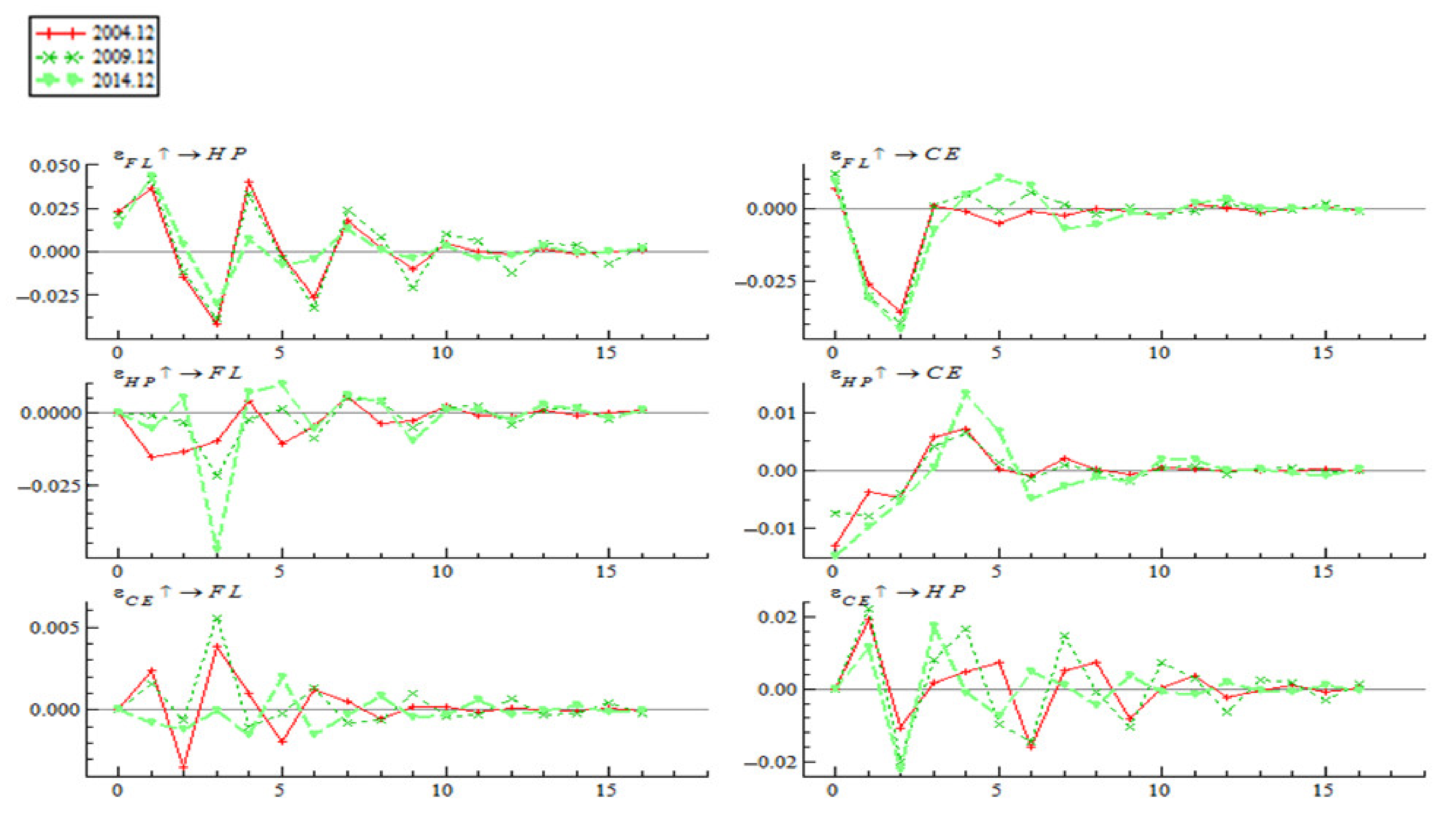
Two different impulse response diagrams can be derived from TVP-VAR model, with one for time point impulse responses as shown in Figure 3 and the other for period impulse responses as shown in Figure 4. The time points in Figure 3 are December 2004, December 2009, and December 2014, which were randomly selected, while the lead times in Figure 4 are set as 1-period ahead, 3-period ahead, and 5-period ahead. Figure 4 indicates impulse responses formed by a unit of standard forward shock at different lead times.
① Analysis of the Time-Variant Characteristics of Impulse Responses at Different Time Points
Impulse response functions of three shocks at three time points showed similar changes. To be specific, house price reacted to the shock of financial leverage in the current period. Its intensity reached a maximum in period 1, then declined rapidly and reached a minimum in period 3, then fluctuated at an increasingly smaller range, and finally showed almost no volatility in period 9. Similarly, consumer expenditure responded to financial leverage in the current period. Its intensity fell rapidly after that, reaching a minimum in period 3, and then gradually increased and approached zero in period 6. Financial leverage responded to the shock of house price in the current period. Its intensity gradually decreased after that, reaching a minimum in period 3, and then gradually increased and got close to zero in period 6. Consumer expenditure responded to house price in the current period. Its intensity reached a minimum in the current period, then gradually increased, reaching a maximum in period 4, and then approached zero in period 9. Impulse response functions of the shock of house price on consumer expenditure at three time points showed similar trends. The value of impulse responses of house price switched between positive and negative ranges and approached zero in period 12.
Impulse responses of financial leverage to consumer expenditure were not consistent at the three time points. Specifically, the impulse response of financial leverage to consumer expenditure in December 2014 was quite different from the impulse responses in December 2004 and December 2009. Impulse responses of financial leverage to consumer expenditure in December 2004 and December 2009 gradually declined and reached a minimum in period 3, rose rapidly and became positive in period 4, and then gradually fell to zero. Financial leverage immediately responded to consumer expenditure in December 2014. Its intensity gradually decreased, reached a minimum in period 4, and then gradually rose and got close to zero in period 10.
② Analysis of Time-variant Characteristics of Impulse Response at Different Lead Times
Figure 3 shows impulse responses formed by a unit of standard forward shock at 1-period ahead, 3-period ahead, and 5-period ahead. Although impulse responses at three different lead times are generally similar, they are different in direction.
As shown in Figure 4, impulse responses of house price to financial leverage at 1-period ahead are positive and very stable. This means that empirical data reveal that a rise in financial leverage in China will significantly stimulate a rise in house price. Impulse responses of consumer expenditure to financial leverage at 1-period ahead were always negative, a trend that further expanded after 2006. Impulse responses of financial leverage to house price at 1-period ahead, 3-period ahead, and 5-period ahead showed a similar trend and were negative most of the time. Impulse responses of consumer expenditure to house price at 1-period ahead were negative and very stable. Impulse responses at 1-period ahead, 3-period ahead, and 5-period ahead were negative at an expanded trend in 2005, 2010, and 2015, which shows that the inhibitory effect of house price on consumer expenditure became more obvious over time. In addition, impulse responses of financial leverage to consumer expenditure at 1-period ahead were positive most of the time, while responses of house price to consumer expenditure were always positive.
So far, this study has analyzed the internal relation and transmission mechanism among financial leverage, house price, and consumer expenditure with the help of the TVP-SV-VAR model against the realistic background that China is undergoing major changes in economic structure and verified hypothesis 1. To further analyze the dynamic correlation among them, we measure the coefficients of dynamic correlation among them with the Bayesian DCC-GARCH model.
4.2. Empirical Analysis Based on the Bayesian DCC-GARCH Model
4.2.1. Estimation Results of the Model
The Bayesian DCC-GARCH model was used to analyze the dynamic correlation among financial leverage, house price, and consumer expenditure. Table 2 presents the empirical results of the model.
Parameter measures the skewness of financial leverage, house price, and consumer expenditure. means right-skewed, while ≤ 1 means left-skewed. is a constant term of the variance equation of the model. α and β are the coefficients of ARCH term and GARCH term of the variance equation, respectively; the closer their sum is to 1, the slower is the decay rate of the volatility. In addition, measures whether the thick-tail distribution is applicable to the error term. a and b and their sum are used to detect whether the DCC model should be employed. If , the CCC model is applicable. If , the DCC model is more suitable. As seen in Table 2, it is reasonable to use the DCC model for analysis.
Estimation results of the model show that the volatility of financial leverage, house price, and consumer expenditure is asymmetric, with financial leverage and consumer expenditure obviously left-skewed and house price right-skewed. Being left-skewed means that volatility has a higher probability of falling to the right of the mean value, while being right-skewed means volatility has a higher probability of falling to the left of the mean value. Assuming volatility is a risk, being left-skewed indicates greater market risk. The asymmetry of volatility shows that the risk of volatility in financial leverage and consumer expenditure is relatively large and that of volatility in house price is relatively small. The mean value of of the three variables is above 0.27. Volatility in financial leverage, house price, and consumer expenditure gradually intensifies at a slower speed, which indicates its strong inertia.
4.2.2. Analysis of Dynamic Correlation Coefficients
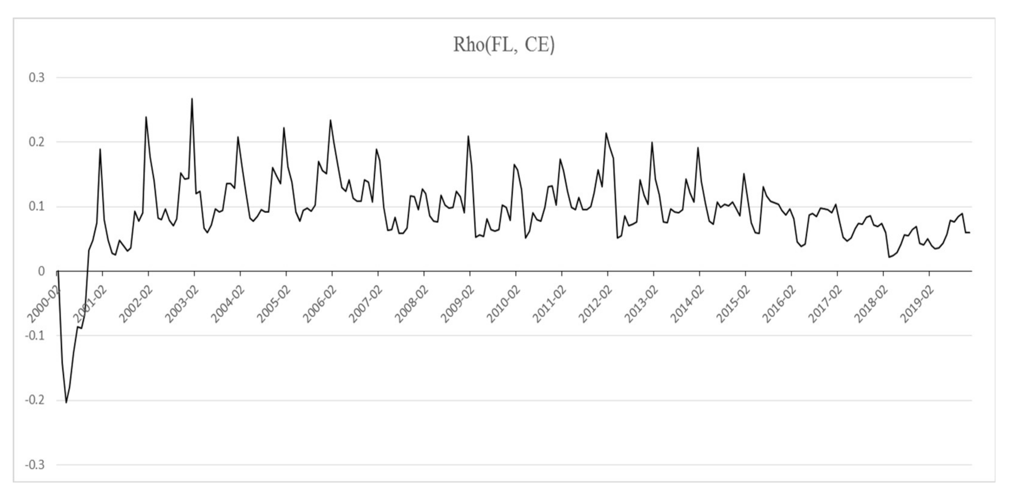
Figure 5, Figure 6 and Figure 7 show a dynamic correlation between financial leverage and house price, financial leverage and consumer expenditure, and house price and consumer expenditure, respectively, calculated using the Bayesian DCC-GARCH model. We can draw the following conclusions from them:
First, the coefficient of dynamic correlation between financial leverage and house price was negative in 2000 and from 2011 to 2015 and positive during the rest of the time period. Its value varied between –0.1514 and 0.1199. In terms of time trend, it showed an upward trend from 2000 to 2005 and a downward trend from 2007 to 2008. It rebounded rapidly from the beginning of 2008, reaching a maximum in 2009; then dropped rapidly again, reaching a minimum in 2012; rebounded again, reaching another maximum in the first half of 2017; and dropped at a slower speed from the second half of 2017, which shows that financial deleveraging has gradually reduced the correlation between financial leverage and house price. Second, the coefficient of dynamic correlation between financial leverage and consumer expenditure was negative from February 2000 to September 2000 and positive after October 2000, ranging from 0.0594 to 0.2699. Overall, there is a positive correlation between them. Figure 6 indicates that the coefficient declined significantly after 2015, which reveals that over time, the positive effect of financial leverage on consumer expenditure has gradually decreased. In addition, the coefficient shows obvious cyclical volatility with change in seasons. Most of the cyclic climaxes occurred in January each year, near the traditional Chinese Spring Festival, which indicates that the influence of the festival on the correlation between financial leverage and consumer expenditure cannot be ignored. Third, the coefficient of dynamic correlation between house price and consumer expenditure was always negative, varying from –0.0992 to –0.3035. This shows there is a negative correlation between house price and consumer expenditure, which indicates that rising house prices will restrain increase in consumer expenditure. From the perspective of time trend, the correlation showed a generally downward trend from 2000 to 2019. Especially from 2017 to 2018, the downward trend was very obvious. This may have resulted from the implementation of the “three-year plan for redeveloping shantytowns” and monetary resettlement compensation policy beginning from 2015, which quickly stimulated a rise in house prices in China’s third- and fourth-tier cities, which drove the country’s average house price to rise again and led to a rapid decline in consumer expenditure. We can conclude that with the vigorous development of China’s real estate market, the rapid rise in house prices weakens the increase in consumer expenditure to a certain extent and that this inhibitory effect becomes more obvious over time.
Figure 5, Figure 6 and Figure 7 indicate house price and consumer expenditure are most relevant, followed by financial leverage and consumer expenditure, and then by financial leverage and house price and these empirical analysis result confirm hypothesis 2. The dynamic correlations among financial leverage, house price, and consumer expenditure are as follows: a negative correlation between house price and consumer expenditure, a positive correlation between financial leverage and consumer expenditure, and an uncertain relationship between financial leverage and house price. This means that currently, a rise in financial leverage helps stimulate consumer expenditure, while a continued rise in house prices gradually reduces consumer expenditure.
5. Conclusions and Discussion
5.1. Conclusions
A continued rapid rise in China’s house prices and intensified volatility in consumer expenditure have attracted more and more attention from academic and practical circles. This study first analyzes the mechanism of action and transmission among China’s financial leverage, house price, and consumer expenditure in recent years by constructing a TVP-SV-VAR model with both time-variant parameters and stochastic volatility (Figure 8 shows the interaction of financial leverage, house price, and consumer expenditure). The results show that a rise in financial leverage significantly increases house prices and reduces consumer expenditure, and it is not difficult to find out that this result is consistent with the results in recently published literature, such as Mian et al. (2017) and Verner and Gyöngyösi (2020) [40,61], but is inconsistent with Gao et al. (2020) and Ruan et al. (2020) [35,36]. In contrast to Burrows (2018) and Cloyne et al. (2019) [46,47], the results show that a rise in house prices inhibits financial leverage and weakens consumer expenditure. It means that the wealth effect of the housing market is not significant in China [48]. Besides, similar to Yin et al., (2021), the results also show that an increase in consumer expenditure raises the level of financial leverage and stimulates the rise in house prices [62].
Secondly, the study further explores the dynamic correlation among financial leverage, house price, and consumer expenditure with the help of the DCC-GARCH model. The results show that there is a negative correlation between house price and consumer expenditure, a positive correlation between financial leverage and consumer expenditure, and an uncertain relationship between financial leverage and house price and that house price and consumer expenditure are most relevant, followed by financial leverage and consumer expenditure, and then by financial leverage and house price. Combined with the two models, we can find out that in the current year, the credit increase raised by financial leverage stimulated the current consumption. This short-term stimulating effect will turn into an inhibitory effect after one to two years since households need to repay the credit by reducing their expenditures. House price inhibits households’ expenditures due to the budget limit, while the increases in expenditure reflect a higher income expectation, which increases the demand for houses. This indicates that the demand for houses of Chinese families is still an inelastic demand.
Our study uses macrodata to dig into the dynamic relationship among house price, financial leverage, and consumer expenditure in China. However, due to a lack of data, we cannot track the household-level information about consumption and credits although heterogeneity cannot be ignored. Low-income and high-income families have different consuming behaviors and preferences for investment. For example, in China, most low-income households choose to save for the future while high-income households tend to allocate financial assets. The geographic factor also influences house price trends. Due to an imbalance in the allocation of public resources, the migration of a large population to cities has caused different changes in rural and urban housing prices and house prices in rural areas are more sensitive to economic shock. In this case, in our future research, geographic and income heterogeneity could be considered in the model to investigate different paths of effects.
5.2. Discussion
China is at a critical stage of economic transformation and upgrading. It is important to maintain relatively stable consumer expenditure. However, continued rapid rises in house prices have not only increased the debt pressure on residents and decreased their living standards but also led to a deteriorated non-performing loan ratio of the credit sector to a certain extent. These factors are not conducive to the transformation and upgrading of China’s economic growth mode. This study reveals that there is a close relationship among financial leverage, house price, and consumer expenditure. Therefore, we believe that to achieve a balanced economic growth inside and outside China, potential impacts of financial leverage should be fully considered in maintaining the stability of consumer expenditure and formulating housing price control policies and monetary and macroprudential policies should be employed to effectively control the overall gate of the leverage ratio, thereby achieving a balanced and stable development of the macroeconomy.
Author Contributions
Conceptualization, K.D. and S.W.; methodology, K.D.; software, S.W.; validation, K.D., S.W. and X.L.; formal analysis, K.D.; investigation, S.W.; resources, S.W.; data curation, X.L.; writing—original draft preparation, K.D.; writing—review and editing, K.D.; visualization, C.-T.C.; supervision, C.-T.C.; project administration, S.W.; funding acquisition, C.-T.C. All authors have read and agreed to the published version of the manuscript.
Funding
This research was supported by the National Natural Science Foundation of China No. 71901002; The Ministry of Science and Technology under Grant MOST 106-2410-H-182-004 and Chang Gung Medical Foundation under Grant BMRPA79; General Project of Philosophy and Social Sciences in Jiangsu Universities No.2019sja0411; NanJing Xiaozhuang University High Level Cultivation Project No.2018nxy05.
Institutional Review Board Statement
Not applicable.
Informed Consent Statement
Not applicable.
Data Availability Statement
Not applicable.
Conflicts of Interest
The authors declare no conflict of interest.
References
- Xu, H. Sustainable Development of China’s Economy under the “New Normal”. China Dev. Observ. 2014, 9, 21–25. [Google Scholar]
- Lamont, O.; Stein, J.C. Leverage and house-price dynamics in US cities. Rand J. Econ. 1999, 30, 498–514. [Google Scholar] [CrossRef] [Green Version]
- Aizenman, J.; Jinjarak, Y. Real estate valuation, current account and credit growth pat terns, before and after the 2008–2009 crisis. J. Int. Money Financ. 2014, 48, 249–270. [Google Scholar] [CrossRef] [Green Version]
- Wang, Y.; Du, L.; Zeng, Z. Special report 4: The current situation, problems and Countermeasures of the coordination of China’s macro-control departments. Econ. Res. Ref. 2014, 4, 60–69. [Google Scholar]
- Bemanke, B.; Gertler, M. Agency costs, net worth, and business fluctuations. Am. Econ. Rev. 1989, 79, 14–31. [Google Scholar]
- Bernanke, B.S.; Gertler, M.; Gilchrist, S. The financial accelerator in a quantitative business cycle framework. Handb. Macroecon. 1999, 1, 1341–1393. [Google Scholar]
- Gertler, M.; Karadi, P. A model of unconventional monetary policy. J. Monet. Econ. 2011, 58, 17–34. [Google Scholar] [CrossRef]
- Herring, R.J.; Wachter, S.M. Real estate booms and banking busts: An international perspective. In The Wharton School Research Paper No. 99-27; The Wharton School, University of Pennsylvania: Philadelphia, PA, USA, 1999; p. 110. [Google Scholar]
- Krugman, P. Balance sheets, the transfer problem, and financial crises. In International Finance and Financial Crises; Springer: Dordrecht, The Netherlands, 1999; pp. 31–55. [Google Scholar]
- Edelstein, R.H.; Paul, J. Japanese land prices: Explaining the boom-bust cycle. In Asia’s Financial Crisis and the Role of Real Estate; Mera, K., Renaud, B., Eds.; Routledge: Milton Park, UK, 2000; pp. 65–82. [Google Scholar]
- Schularick, M.; Taylor, A.M. Credit booms gone bust: Monetary policy, leverage cycles, and financial crises, 1870–2008. Am. Econ. Rev. 2012, 102, 1029–1061. [Google Scholar] [CrossRef] [Green Version]
- Carlin, W.; Soskice, D. How should macroeconomics be taught to undergraduates in the post-crisis era? A concrete proposal. VoxEU. Org. 2012, 1990, 1–3. [Google Scholar]
- Geanakoplos, J.; Zame, W.R. Collateral equilibrium, I: A basic framework. Econ. Theory 2014, 56, 443–492. [Google Scholar] [CrossRef]
- Punzi, M.T. Housing market and current account imbalances in the international economy. Rev. Int. Econ. 2013, 21, 601–613. [Google Scholar] [CrossRef] [Green Version]
- Gete, P.; Reher, M. Two Extensive Margins of Credit and Loan-to-Value Policies. J. Money Credit. Bank. 2016, 48, 1397–1438. [Google Scholar] [CrossRef]
- Mishkin, F.S. Illiquidity, consumer durable expenditure, and monetary policy. Am. Econ. Rev. 1976, 66, 642–654. [Google Scholar]
- Bacchetta, P.; Gerlach, S. Consumption and credit constraints: International evidence. J. Monet. Econ. 1997, 40, 207–238. [Google Scholar] [CrossRef]
- Dynan, K.; Mian, A.; Pence, K.M. Is a Household Debt Overhang Holding Back Consumption? [with comments and discussion]. In Brookings Papers on Economic Activity. JSTOR. 2012, p. 299. Available online: http://0-www-jstor-org.brum.beds.ac.uk/stable/23287219 (accessed on 3 April 2020).
- Dynan, K.; Edelberg, W. The relationship between leverage and household spending behavior: Evidence from the 2007–2009 survey of consumer finances. Fed. Reserve Bank St. Louis Rev. 2013, 95, 425–448. [Google Scholar] [CrossRef] [Green Version]
- Johnson, K.W.; Li, G. Do High Debt Payments Hinder Household Consumption Smoothing? (No. 2007-52); Board of Governors of the Federal Reserve System (US): Washington, DC, USA, 2007. [Google Scholar]
- Baker, S.R. Debt and the Consumption Response to Household Income Shocks. Available online: https://web.stanford.edu/~srbaker/Papers/Baker_DebtConsumption.pdf (accessed on 9 March 2020).
- Mian, A.; Rao, K.; Sufi, A. Household balance sheets, consumption, and the economic slump. Q. J. Econ. 2013, 128, 1687–1726. [Google Scholar] [CrossRef]
- Yao, J.; Fagereng, A.; Natvik, G. Housing, debt and the marginal propensity to consume. Nor. Bank Res. Pap. 2015, pp. 1–38. Available online: http://www.good2use.com/knet/economic/gloss/iaae2016-171.pdf (accessed on 3 April 2020).
- Case, K.E.; Quigley, J.M.; Shiller, R.J. Comparing wealth effects: The stock market versus the housing market. BE J. Macroecon. 2005, 5, 1–34. [Google Scholar] [CrossRef]
- Carroll, C.D.; Otsuka, M.; Slacalek, J. How large are housing and financial wealth effects? A new approach. J. Money Credit Bank. 2011, 43, 55–79. [Google Scholar] [CrossRef] [Green Version]
- Mian, A.; Sufi, A. The consequences of mortgage credit expansion: Evidence from the US mortgage default crisis. Q. J. Econ. 2009, 124, 1449–1496. [Google Scholar] [CrossRef]
- De Bonis, R.; Silvestrini, A. The effects of financial and real wealth on consumption: New evidence from OECD countries. Appl. Financ. Econ. 2012, 22, 409–425. [Google Scholar] [CrossRef] [Green Version]
- Cristini, A.; Sevilla, A. Do House Prices Affect Consumption? A Re-assessment of the Wealth Hypothesis. Economica 2014, 81, 601–625. [Google Scholar] [CrossRef] [Green Version]
- Catte, P.; Girouard, N.; Price, R.; André, C. Housing Markets, Wealth and the Business Cycle (No. 394); OECD Publishing: Paris, France, 2004. [Google Scholar] [CrossRef]
- Campbell, J.Y.; Cocco, J.F. How do house prices affect consumption? Evidence from micro data. J. Monet. Econ. 2007, 54, 591–621. [Google Scholar] [CrossRef] [Green Version]
- Chamon, M.D.; Prasad, E.S. Why are saving rates of urban households in China rising? Am. Econ. J. Macroecon. 2010, 2, 93–130. [Google Scholar] [CrossRef] [Green Version]
- McKinnon, R.I. Money and Capital in Economic Development; Brookings Institution Press: Washington, DC, USA, 1973. [Google Scholar]
- Shaw, E.S. Financial Deepening in Economic Development; Oxford University Press: Oxford, UK, 1973. [Google Scholar]
- Lambertini, L.; Mendicino, C.; Punzi, M.T. Leaning against boom–bust cycles in credit and housing prices. J. Econ. Dyn. Control 2013, 37, 1500–1522. [Google Scholar] [CrossRef] [Green Version]
- Gao, D.; Yue, Q.; Yang, D.; Deng, D.; Xu, G. The effect of residents’ leverage ratio on consumption: Promotion or inhibition. Economist 2020, 8, 100–109. [Google Scholar]
- Ruan, J.; Liu, X.; Ye, H. Research on the current situation and influencing factors of China’s residents’ leverage ratio. Financ. Res. 2020, 8, 18–33. [Google Scholar]
- Ma, E.; Zubairy, S. Homeownership and Housing Transitions: Explaining the Demographic Composition. Available online: https://0-onlinelibrary-wiley-com.brum.beds.ac.uk/doi/10.1111/iere.12493 (accessed on 7 July 2020).
- Fisher, I. The debt-deflation theory of great depressions. Econometrica 1933, 1, 337–357. [Google Scholar] [CrossRef] [Green Version]
- Tobin, J. Keynesian models of recession and depression. Am. Econ. Rev. 1975, 65, 195–202. [Google Scholar]
- Mian, A.; Sufi, A.; Verner, E. Household debt and business cycles worldwide. Q. J. Econ. 2017, 132, 1755–1817. [Google Scholar] [CrossRef]
- Scholnick, B. Consumption smoothing after the final mortgage payment: Testing the magnitude hypothesis. Rev. Econ. Stat. 2013, 95, 1444–1449. [Google Scholar] [CrossRef]
- Mendoza, E.G. Sudden stops, financial crises, and leverage. Am. Econ Rev. 2010, 100, 1941–1966. [Google Scholar] [CrossRef]
- Friedman, M. A Theory of the Consumption Function; Princeton University Press: Princeton, NJ, USA, 1957. [Google Scholar]
- Ando, A.; Modigliani, F. The” life cycle” hypothesis of saving: Aggregate implications and tests. Am. Econ Rev. 1963, 53, 55–84. [Google Scholar]
- De Veirman, E.; Duncan, A. Does wealth variation matter for consumption? Reserve Bank N. Zeal. 2010. Available online: http://citeseerx.ist.psu.edu/viewdoc/download?doi=10.1.1.691.4961&rep=rep1&type=pdf (accessed on 16 July 2020).
- Burrows, V. The impact of house prices on consumption in the UK: A new perspective. Economica 2018, 85, 92–123. [Google Scholar] [CrossRef]
- Cloyne, J.; Huber, K.; Ilzetzki, E.; Kleven, H. The effect of house prices on household borrowing: A new approach. Am. Econ Rev. 2019, 109, 2104–2136. [Google Scholar] [CrossRef]
- Wang, X.; Wen, Y. Can Rising Housing Prices Explain China’s High Household Saving Rate? Fed. Reserve Bank St. Louis Work. Paper Series. 2010. Available online: https://papers.ssrn.com/sol3/papers.cfm?abstract_id=1707062 (accessed on 23 July 2020).
- Bernanke, B.; Gertler, M.; Gilchrist, S. The financial accelerator and the flight to quality. Rev. Econ. Stat. 1996, 78, 1–15. [Google Scholar] [CrossRef]
- Oikarinen, E. Interaction between housing prices and household borrowing: The Finnish case. J. Bank. Financ. 2009, 33, 747–756. [Google Scholar] [CrossRef]
- DeFusco, A.A. Homeowner borrowing and housing collateral: New evidence from expiring price controls. J. Financ. 2018, 73, 523–573. [Google Scholar] [CrossRef]
- Sinai, T.; Souleles, N.S. Owner-occupied housing as a hedge against rent risk. Q. J. Econ. 2005, 120, 763–789. [Google Scholar]
- Stiglitz, J. Joseph Stiglitz and why inequality is at the root of the recession. Next Left Website. 2009. Available online: http://www.nextleft.org/2009/01/joseph-stiglitz-and-why-inequality-is.html (accessed on 3 May 2020).
- Barba, A.; Pivetti, M. Rising household debt: Its causes and macroeconomic implications—a long-period analysis. Camb. J. Econ. 2009, 33, 113–137. [Google Scholar] [CrossRef] [Green Version]
- Primiceri, G.E. Time varying structural vector autoregressions and monetary policy. Rev. Econ. Stud. 2005, 72, 821–852. [Google Scholar] [CrossRef]
- Engle, R. Dynamic conditional correlation: A simple class of multivariate generalized autoregressive conditional heteroskedasticity models. J. Bus. Econ. Stat. 2002, 20, 339–350. [Google Scholar] [CrossRef]
- Christodoulakis, G.A.; Satchell, S.E. Correlated ARCH (CorrARCH): Modelling the time-varying conditional correlation between financial asset returns. Eur. J. Oper. Res. 2002, 139, 351–370. [Google Scholar] [CrossRef]
- Nakajima, J. Time-Varying Parameter VAR Model with Stochastic Volatility: An Overview of Methodology and Empirical Applications (No. 11-E-09); Institute for Monetary and Economic Studies, Bank of Japan: Tokyo, Japan, 2011. [Google Scholar]
- Fioruci, J.A.; Ehlers, R.S.; Andrade Filho, M.G. Bayesian multivariate GARCH models with dynamic correlations and asymmetric error distributions. J. Appl. Stat. 2014, 41, 320–331. [Google Scholar] [CrossRef]
- Bauwens, L.; Laurent, S. A new class of multivariate skew densities, with application to generalized autoregressive conditional heteroscedasticity models. J. Bus Econ. Stat. 2005, 23, 346–354. [Google Scholar] [CrossRef]
- Verner, E.; Gyöngyösi, G. Household debt revaluation and the real economy: Evidence from a foreign currency debt crisis. Am. Econ. Rev. 2020, 110, 2667–2702. [Google Scholar] [CrossRef]
- Yin, Z.; Li, Q.; Zhang, C. The impact of income inequality on household leverage. Financ. Trade Econ. 2021, 1, 11–15. [Google Scholar]
Figure 1.
The relationship among China’s major macroeconomic sectors.

Figure 2.
Estimation results of parameters in the TVP-SV-VAR model.

Figure 3.
Impulse responses to shocks at different time points.

Figure 4.
Impulse responses to shocks at different lead times.
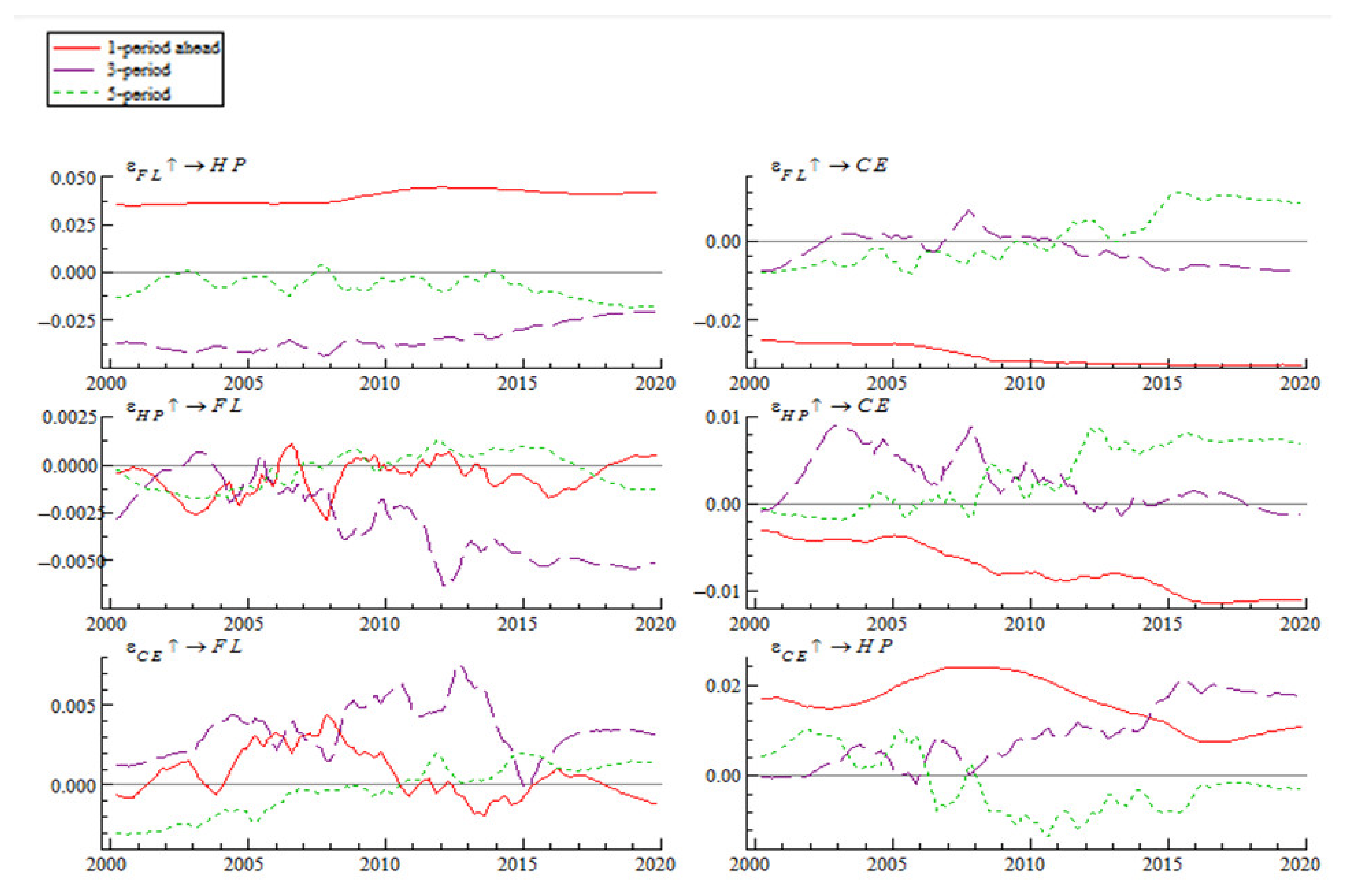
Figure 5.
Diagram of the coefficient of dynamic correlation between financial leverage and house price.
Figure 5.
Diagram of the coefficient of dynamic correlation between financial leverage and house price.
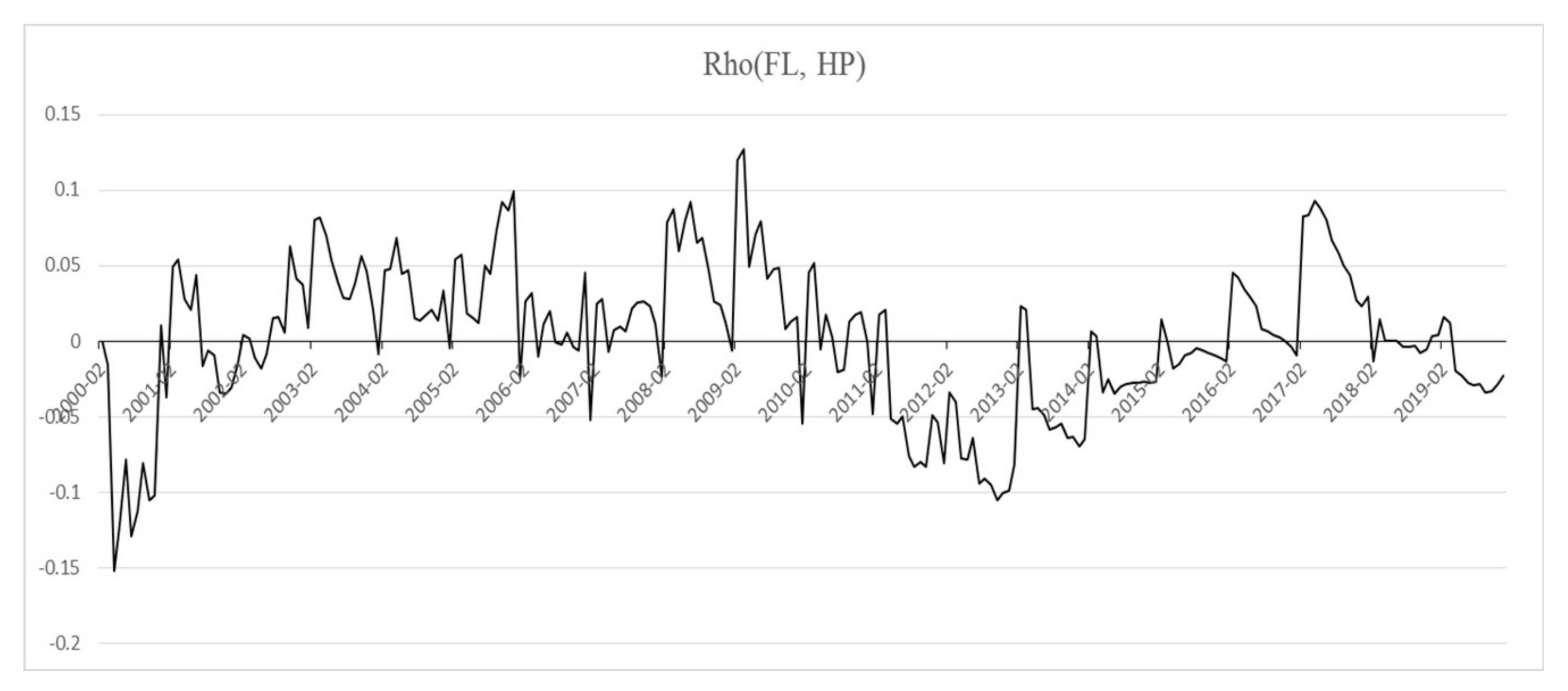
Figure 6.
Diagram of the coefficient of dynamic correlation between financial leverage and consumer expenditure.
Figure 6.
Diagram of the coefficient of dynamic correlation between financial leverage and consumer expenditure.

Figure 7.
Diagram of the coefficient of dynamic correlation between house price and consumer expenditure.
Figure 7.
Diagram of the coefficient of dynamic correlation between house price and consumer expenditure.
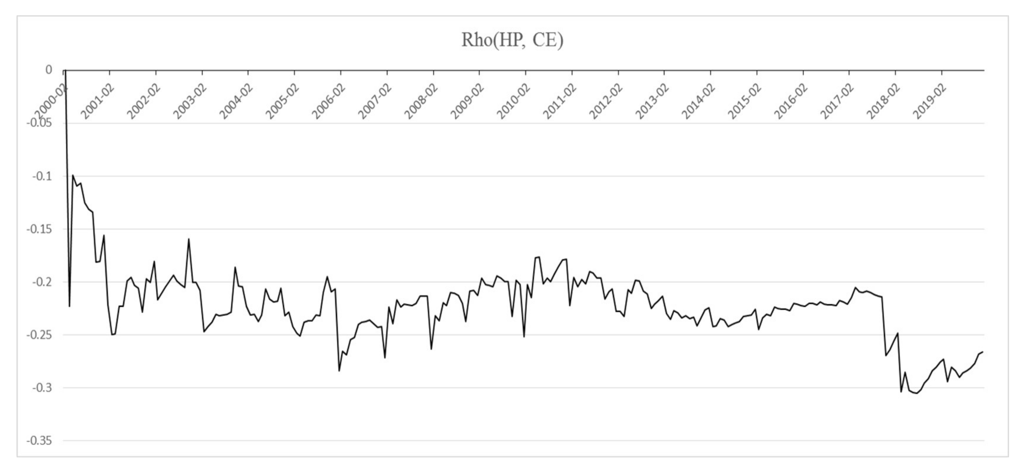
Figure 8.
Diagram of the interaction of financial leverage, house price, and consumer expenditure.

Table 1.
Estimation results of the time-varying parameter vector autoregression with stochastic volatility (TVP-SV-VAR) model.
Table 1.
Estimation results of the time-varying parameter vector autoregression with stochastic volatility (TVP-SV-VAR) model.
| Parameter | Mean Value | Standard Deviation | 95% Confidence Interval | Geweke | Non-Effective Factor |
|---|---|---|---|---|---|
| sb1 | 0.0229 | 0.0026 | [0.0184, 0.0287] | 0.05 | 13.01 |
| sb2 | 0.0208 | 0.0021 | [0.0171, 0.0253] | 0.81 | 9.99 |
| sa1 | 0.0903 | 0.0435 | [0.0428, 0.2086] | 0.405 | 149.21 |
| sa2 | 0.0743 | 0.0249 | [0.0412, 0.1314] | 0.816 | 81.91 |
| sh1 | 0.5188 | 0.062 | [0.4130, 0.6568] | 0.001 | 57.02 |
| sh2 | 0.5949 | 0.1496 | [0.3393, 0.9272] | 0.272 | 71.59 |
Table 2.
Results of the Monte Carlo estimation of the Bayesian dynamic conditional correlational autoregressive conditional heteroscedasticity (Bayesian DCC-GARCH) model.
Table 2.
Results of the Monte Carlo estimation of the Bayesian dynamic conditional correlational autoregressive conditional heteroscedasticity (Bayesian DCC-GARCH) model.
| Quantile | |||||||
|---|---|---|---|---|---|---|---|
| Variable | Parameter | Mean Value | 2.50% | 25.00% | 50.00% | 75.00% | 97.50% |
| FL | 0.5629 | 0.5048 | 0.5314 | 0.5479 | 0.5688 | 0.9255 | |
| 0.0021 | 0.0002 | 0.0003 | 0.0004 | 0.0005 | 0.0434 | ||
| 0.2651 | 0.0651 | 0.1818 | 0.2520 | 0.3392 | 0.5110 | ||
| 0.3172 | 0.0331 | 0.1718 | 0.2520 | 0.3392 | 0.5110 | ||
| HP | 1.0096 | 0.9807 | 0.9976 | 1.0067 | 1.0213 | 1.0445 | |
| 0.0042 | 0.0018 | 0.0028 | 0.0036 | 0.0046 | 0.0117 | ||
| 0.3696 | 0.0606 | 0.2405 | 0.3639 | 0.4839 | 0.7355 | ||
| 0.3464 | 0.1168 | 0.2326 | 0.3164 | 0.4305 | 0.8066 | ||
| CE | 0.9407 | 0.8622 | 0.9060 | 0.9347 | 0.9696 | 1.0370 | |
| 0.0048 | 0.0023 | 0.0034 | 0.0040 | 0.0047 | 0.0270 | ||
| 0.0639 | 0.0054 | 0.0262 | 0.0534 | 0.0898 | 0.1858 | ||
| 0.2098 | 0.0161 | 0.0855 | 0.1796 | 0.2916 | 0.6885 | ||
| 0.7859 | 0.2554 | 0.7562 | 0.7959 | 0.8456 | 0.9332 | ||
| 0.0093 | 0.0006 | 0.0031 | 0.0065 | 0.0112 | 0.0387 | ||
| 0.411 | 0.0094 | 0.1222 | 0.3175 | 0.6870 | 0.9726 | ||
Publisher’s Note: MDPI stays neutral with regard to jurisdictional claims in published maps and institutional affiliations. |
© 2021 by the authors. Licensee MDPI, Basel, Switzerland. This article is an open access article distributed under the terms and conditions of the Creative Commons Attribution (CC BY) license (http://creativecommons.org/licenses/by/4.0/).
Share and Cite
MDPI and ACS Style
Dong, K.; Chang, C.-T.; Wang, S.; Liu, X. The Dynamic Correlation among Financial Leverage, House Price, and Consumer Expenditure in China. Sustainability 2021, 13, 2617. https://0-doi-org.brum.beds.ac.uk/10.3390/su13052617
AMA Style
Dong K, Chang C-T, Wang S, Liu X. The Dynamic Correlation among Financial Leverage, House Price, and Consumer Expenditure in China. Sustainability. 2021; 13(5):2617. https://0-doi-org.brum.beds.ac.uk/10.3390/su13052617
Chicago/Turabian StyleDong, Kai, Ching-Ter Chang, Shaonan Wang, and Xiaoxi Liu. 2021. "The Dynamic Correlation among Financial Leverage, House Price, and Consumer Expenditure in China" Sustainability 13, no. 5: 2617. https://0-doi-org.brum.beds.ac.uk/10.3390/su13052617
Note that from the first issue of 2016, this journal uses article numbers instead of page numbers. See further details here.