
Investigating the Causal Relationships among Carbon Emissions, Economic Growth, and Life Expectancy in Turkey: Evidence from Time and Frequency Domain Causality Techniques


Abstract
:1. Introduction
2. Literature Review and Hypotheses Development
2.1. Literature Review
2.2. Theory and Hypotheses
2.2.1. Theory
2.2.2. Hypotheses
3. Data and Methodology
3.1. Data
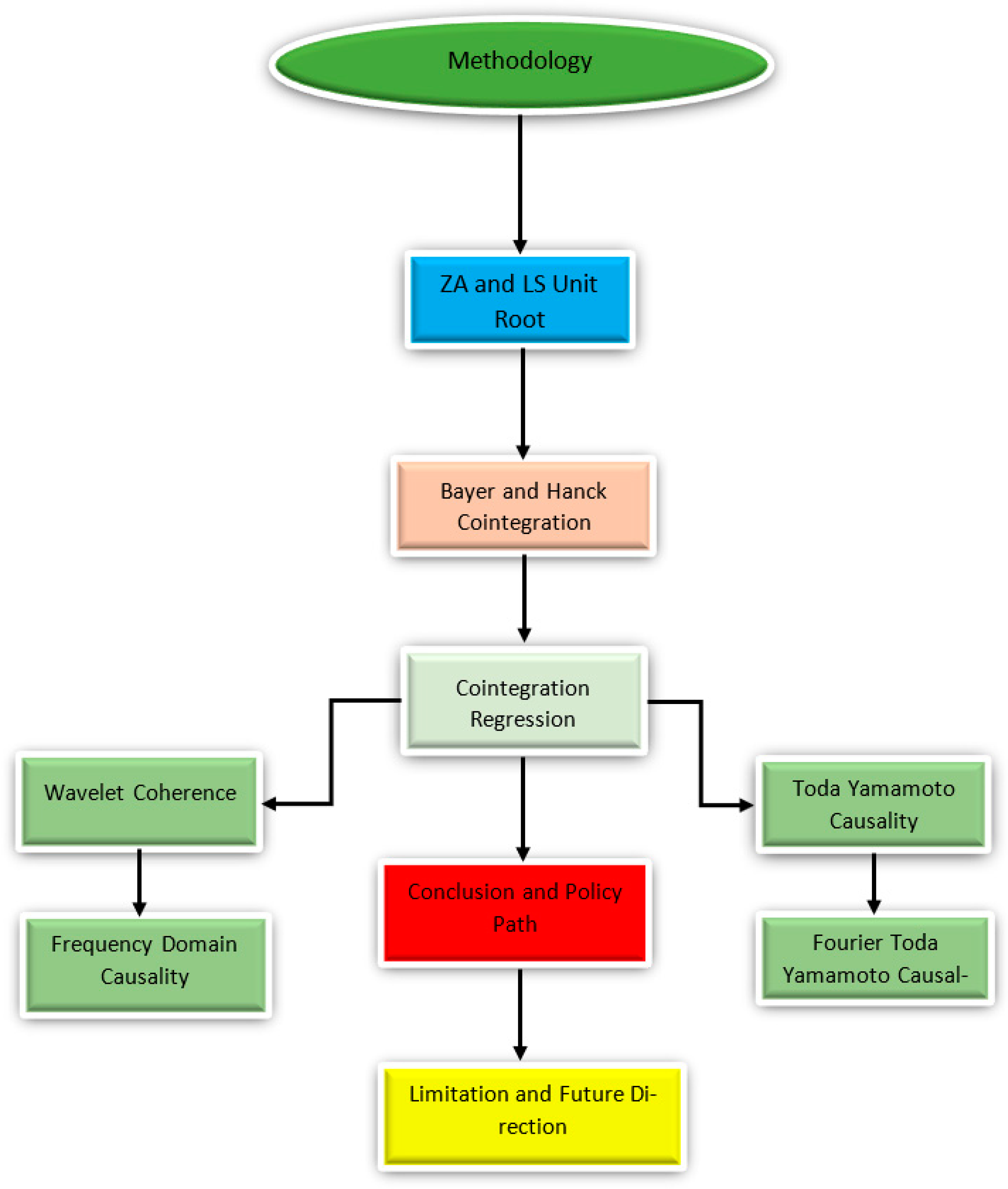
3.2. Methodology
3.2.1. Stationarity Tests
The Zivot–Andrews Unit Root Test
Lee–Strazicich Unit-Root Test
3.2.2. Cointegration Test
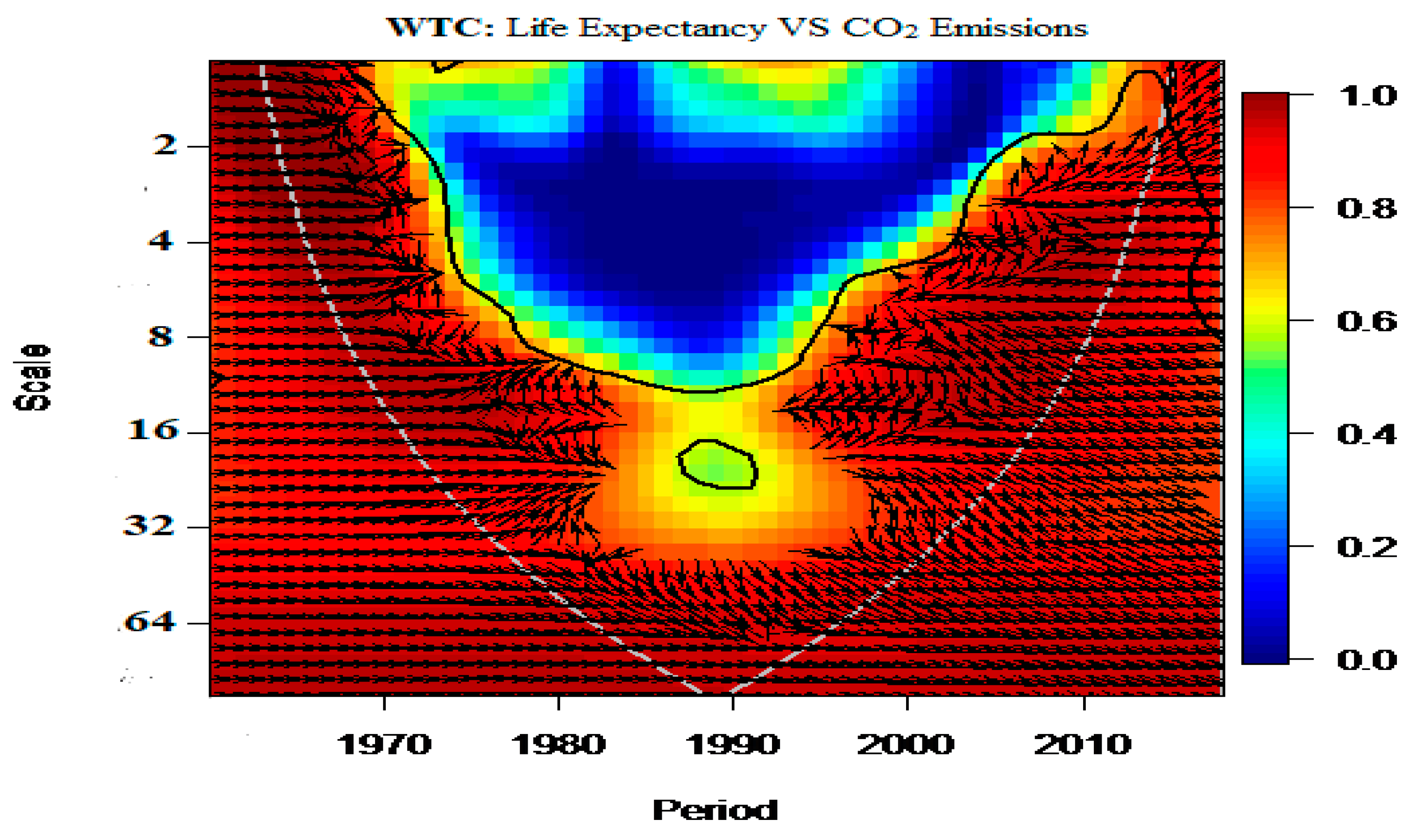
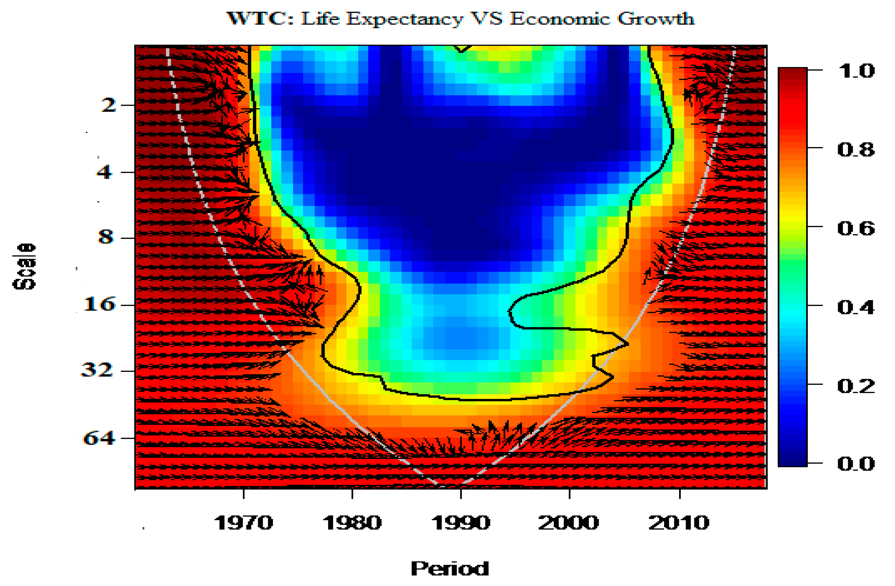
3.2.3. Wavelet Approach
3.2.4. Toda–Yamamoto and Fourier Toda–Yamamoto Causality Tests
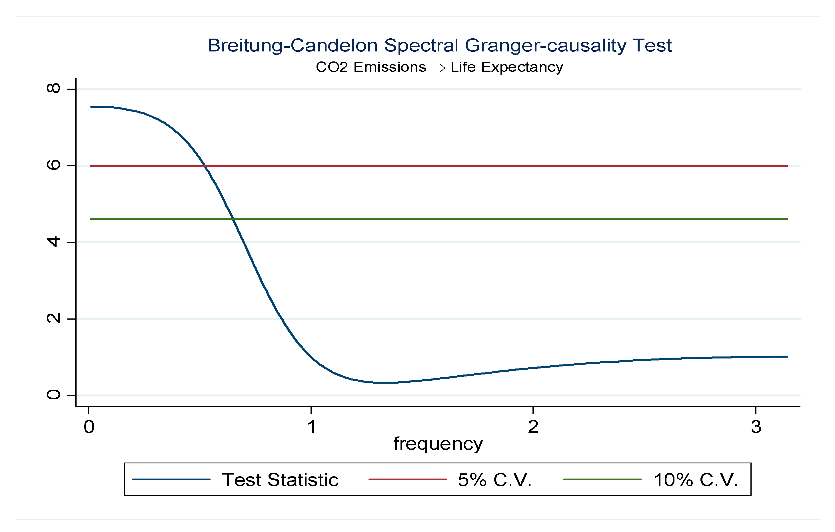
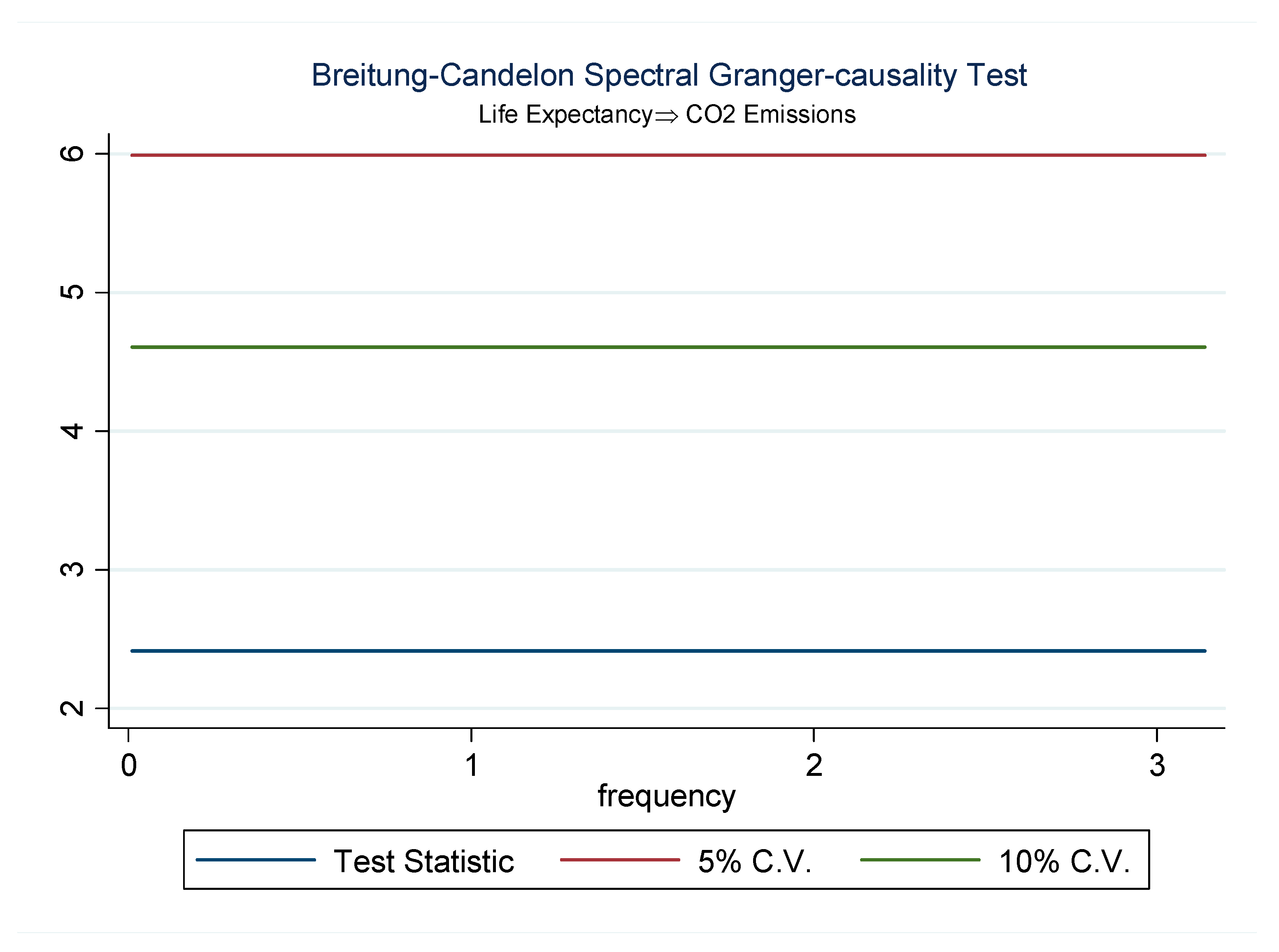
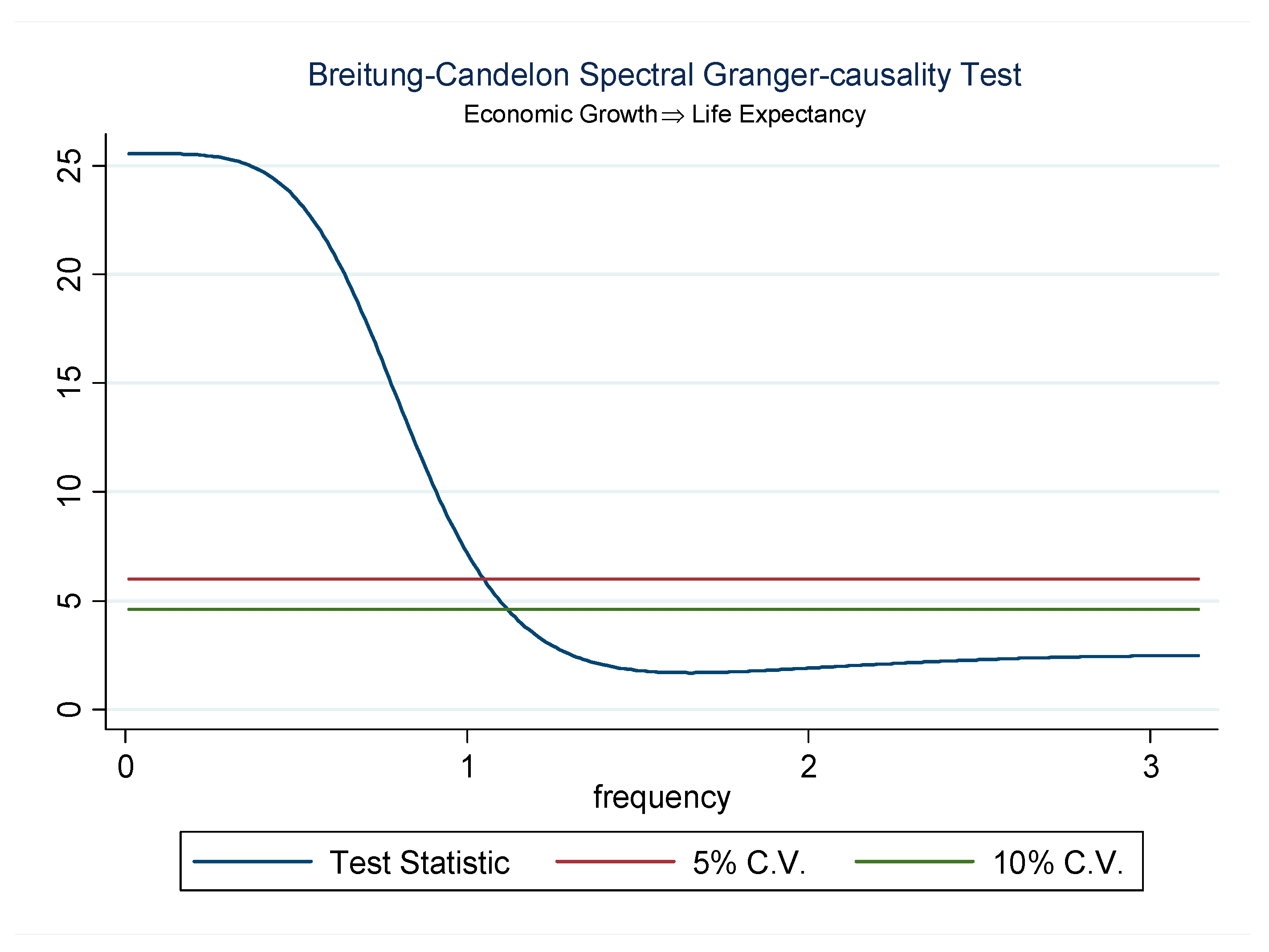
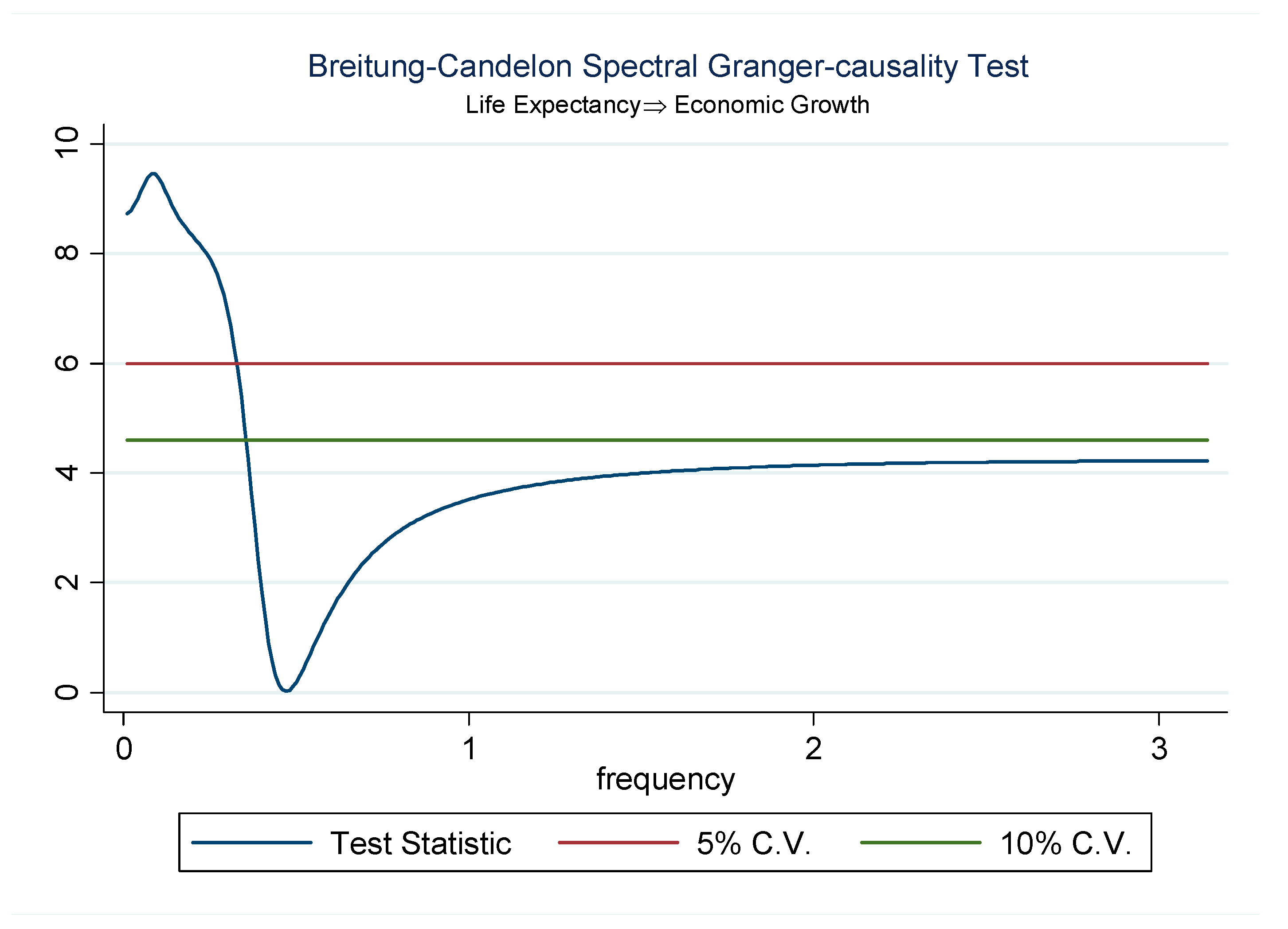
3.2.5. Breitung–Candelon Frequency-Domain Causality TEST
4. Empirical Findings and Inferences
5. Conclusions and Inference
Author Contributions
Funding
Institutional Review Board Statement
Informed Consent Statement
Data Availability Statement
Conflicts of Interest
References
- Balan, F. Environmental quality and its human health effects: A causal analysis for the EU-25. Int. J. Appl. Econ. 2016, 13, 57–71. [Google Scholar]
- Agbanike, T.F.; Nwani, C.; Uwazie, U.; Uma, K.E.; Anochiwa, L.; Igberi, C.; Ogbonnaya, I.O. Oil, Environmental Pollution and Life Expectancy In Nigeria. Appl. Ecol. Environ. Res. 2019, 17, 11143–11162. [Google Scholar] [CrossRef]
- Balakrishnan, K.; Dey, S.; Gupta, T.; Dhaliwal, R.S.; Brauer, M.; Cohen, A.J.; Sabde, Y. The impact of air pollution on deaths, disease burden, and life expectancy across the states of India: The Global Burden of Disease Study 2017. Lancet Planet. Health 2019, 3, e26–e39. [Google Scholar] [CrossRef] [Green Version]
- Schwartz, J.D.; Wang, Y.; Kloog, I.; Yitshak-Sade, M.A.; Dominici, F.; Zanobetti, A. Estimating the effects of PM2.5 on life expectancy using causal modeling methods. Environ. Health Perspect. 2018, 126, 127002. [Google Scholar] [CrossRef] [PubMed] [Green Version]
- Adebayo, T.S.; Odugbesan, J.A. Modeling CO2 emissions in South Africa: Empirical evidence from ARDL based bounds and wavelet coherence techniques. Environ. Sci. Pollut. Res. 2020, 1–13. [Google Scholar] [CrossRef]
- Odugbesan, J.A.; Adebayo, T.S. The symmetrical and asymmetrical effects of foreign direct investment and financial development on carbon emission: Evidence from Nigeria. SN Appl. Sci. 2020, 2, 1–15. [Google Scholar] [CrossRef]
- Rjoub, H.; Odugbesan, J.A.; Adebayo, T.S.; Wong, W.K. Sustainability of the Moderating Role of Financial Development in the Determinants of Environmental Degradation: Evidence from Turkey. Sustainability 2021, 13, 1844. [Google Scholar] [CrossRef]
- Odusanya, I.A.; Adegboyega, S.B.; Kuku, M.A. Environmental Quality and Health Care Spending In Nigeria. Fountain J. Manag. Soc. Sci. 2014, 3, 57–67. [Google Scholar]
- Mariani, F.; Pérez-Barahona, A.; Raffin, N. Life expectancy and the environment. J. Econom. Dyn. Control 2010, 34, 798–815. [Google Scholar] [CrossRef]
- Biyase, M.; Malesa, M. Life Expectancy and Economic Growth: Evidence from the Southern African Development Community. Econ. Internazionale/Int. Econ. 2019, 72, 351–366. Available online: http://www.iei1946.it/en/rivista-articolo.php?id=197 (accessed on 10 December 2020).
- Alam, M.S.; Shahbaz, M.; Paramati, S.R. The role of financial development and economic misery on life expectancy: Evidence from post reforms in India. Soc. Indic. Res. 2016, 128, 481–497. [Google Scholar] [CrossRef]
- Shahbaz, M.; Loganathan, N.; Mujahid, N.; Ali, A.; Nawaz, A. Determinants of life expectancy and its prospects under the role of economic misery: A case of Pakistan. Soc. Indic. Res. 2016, 126, 1299–1316. [Google Scholar] [CrossRef] [Green Version]
- Wu, C. Human capital, life expectancy, and the environment. J. Int. Trade Econ. Dev. 2017, 26, 885–906. [Google Scholar] [CrossRef]
- Wang, Z.; Asghar, M.M.; Zaidi, S.A.H.; Nawaz, K.; Wang, B.; Zhao, W.; Xu, F. The dynamic relationship between economic growth and life expectancy: Contradictory role of energy consumption and financial development in Pakistan. Struct. Chang. Econ. Dyn. 2020, 53, 257–266. [Google Scholar] [CrossRef]
- He, L.; Li, N. The linkages between life expectancy and economic growth: Some new evidence. Empir. Econ. 2020, 58, 2381–2402. [Google Scholar] [CrossRef]
- Kirikkaleli, D.; Adebayo, T.S. Do public-private partnerships in energy and renewable energy consumption matter for consumption-based carbon dioxide emissions in India? Environ. Sci. Pollut. Res. 2021, 1–14. [Google Scholar] [CrossRef]
- World Bank. World Development Indicators. Available online: http://data.worldbank.org/ (accessed on 30 September 2020).
- Bilgen, S.; Keleş, S.; Kaygusuz, A.; Sarı, A.; Kaygusuz, K. Global warming and renewable energy sources for sustainable development: A case study in Turkey. Renew. Sustain. Energy Rev. 2008, 12, 372–396. [Google Scholar] [CrossRef]
- TUIK. Main Statistics. Available online: http://www.turkstat.gov.tr (accessed on 30 May 2020).
- Gövdeli, T. Life Expectancy, Direct Foreign Investments, Trade Openness and Economic Growth in E7 Countries: Heterogeneous Panel Analysis. Third Sect. Soc. Econ. Rev. 2019, 54, 731–743. [Google Scholar] [CrossRef]
- Shahbaz, M.; Shafiullah, M.; Mahalik, M.K. The dynamics of financial development, globalisation, economic growth and life expectancy in sub-Saharan Africa. Aust. Econ. Pap. 2019, 58, 444–479. [Google Scholar] [CrossRef]
- Sirag, A.; Norashidah, M.N.; Law, S.H. Does higher longevity harm economic growth? Panoeconomicus 2020, 67, 51–68. [Google Scholar] [CrossRef] [Green Version]
- Yakita, A. Life expectancy, money, and growth. J. Political Econ. 2006, 19, 579–592. [Google Scholar] [CrossRef]
- Kalemli-Ozcan, S.; Ryder, H.E.; Weil, D.N. Mortality decline, human capital investment, and economic growth. J. Dev. Econ. 2000, 62, 1–23. [Google Scholar] [CrossRef]
- Acemoglu, D.; Johnson, S. Disease and development: The effect of life expectancy on economic growth. J. Political Econ. 2007, 115, 925–985. [Google Scholar] [CrossRef] [Green Version]
- Leung, M.C.; Wang, Y. Endogenous health care, life expectancy and economic growth. Pac. Econ. Rev. 2010, 15, 11–31. [Google Scholar] [CrossRef]
- Boucekkine, R.; La Croix, D.D.; Licandro, O. Vintage human capital, demographic trends, and endogenous growth. J. Econom. Theory 2002, 104, 340–375. [Google Scholar] [CrossRef] [Green Version]
- Echevarría, C.A. Life expectancy, schooling time, retirement, and growth. Econ. Inq. 2004, 42, 602–617. [Google Scholar] [CrossRef]
- Kunze, L. Life expectancy and economic growth. J. Macroecon. 2014, 39, 54–65. [Google Scholar] [CrossRef]
- Martins, F.; Felgueiras, C.; Smitkova, M.; Caetano, N. Analysis of fossil fuel energy consumption and environmental impacts in European countries. Energies 2019, 12, 964. [Google Scholar] [CrossRef] [Green Version]
- Wang, Z.; Asghar, M.M.; Zaidi, S.A.H.; Wang, B. Dynamic linkages among CO2 emissions, health expenditures, and economic growth: Empirical evidence from Pakistan. Environ. Sci. Pollut. Res. 2019, 26, 15285–15299. [Google Scholar] [CrossRef] [PubMed]
- Sarkodie, S.A.; Strezov, V.; Jiang, Y.; Evans, T. Proximate determinants of particulate matter (PM2.5) emission, mortality and life expectancy in Europe, Central Asia, Australia, Canada and the US. Sci. Total Environ. 2019, 683, 489–497. [Google Scholar] [CrossRef]
- Adebayo, T.S.; Kalmaz, D.B. Determinants of CO2 emissions: Empirical evidence from Egypt. Environ. Ecol. Stat. 2021, 1–24. [Google Scholar] [CrossRef]
- Zaidi, S.A.H.; Danish; Hou, F.; Mirza, F.M. The role of renewable and non-renewable energy consumption in CO2 emissions: A disaggregate analysis of Pakistan. Environ. Sci. Pollut. Res. 2018, 25, 31616–31629. [Google Scholar] [CrossRef]
- Bekhet, H.A.; Matar, A.; Yasmin, T. CO2 emissions, energy consumption, economic growth, and financial development in GCC countries: Dynamic simultaneous equation models. Renew. Sustain. Energy Rev. 2017, 70, 117–132. [Google Scholar] [CrossRef]
- Wang, B.; Wang, Z. Imported technology and CO2 emission in China: Collecting evidence through bound testing and VECM approach. Renew. Sustain. Energy Rev. 2018, 82, 4204–4214. [Google Scholar] [CrossRef]
- Zakaria, M.; Bibi, S. Financial development and environment in South Asia: The role of institutional quality. Environ. Sci. Pollut. Res. 2019, 26, 7926–7937. [Google Scholar] [CrossRef]
- Zaidi, S.; Saidi, K. Environmental pollution, health expenditure and economic growth in the Sub-Saharan Africa countries: Panel ARDL approach. Sustain. Cities Soc. 2018, 41, 833–840. [Google Scholar] [CrossRef]
- Al-Mulali, U.; Ozturk, I. The effect of energy consumption, urbanization, trade openness, industrial output, and the political stability on the environmental degradation in the MENA (Middle East and North African) region. Energy 2015, 84, 382–389. [Google Scholar] [CrossRef]
- Issaoui, F.; Toumi, H.; Touili, W. The effects of carbon dioxide emissions on economic growth, urbanization, and welfare. J. Energy Dev. 2015, 41, 223–252. Available online: https://0-www-jstor-org.brum.beds.ac.uk/stable/10.2307/90005938 (accessed on 10 December 2020).
- Clootens, N. Public debt, life expectancy, and the environment. Environ. Modeling Assess. 2017, 22, 267–278. [Google Scholar] [CrossRef]
- Ono, T.; Maeda, Y. Sustainable development in an aging economy. Environ. Dev. Econ. 2002, 7, 9–22. [Google Scholar] [CrossRef] [Green Version]
- Pecchenino, R.; Pollard, P. The effects of annuities, bequests and aging in an overlapping generations model of endogenous growth. Econ. J. 1997, 107, 26–46. [Google Scholar] [CrossRef] [Green Version]
- John, A.; Pecchenino, R. An overlapping generations model of growth and the environment. Econ. J. 1994, 104, 1393. [Google Scholar] [CrossRef]
- Elo, I.T.; Preston, S.H. Effects of early-life conditions on adult mortality: A review. Popul. Index 1992, 58, 186–212. Available online: https://0-www-jstor-org.brum.beds.ac.uk/stable/3644718 (accessed on 10 December 2020). [CrossRef] [PubMed]
- Pope, C.A.; Burnett, R.T.; Thurston, G.D.; Thun, M.J.; Calle, E.E.; Krewski, D.; Godleski, J.J. Cardiovascular mortality and longterm exposure to particulate air pollution: Epidemiological evidence of general pathophysiological pathways of disease. Circulation 2004, 109, 71–77. [Google Scholar] [CrossRef] [PubMed] [Green Version]
- Evans, M.F.; Smith, V.K. Do new health conditions support mortality-air pollution effects? J. Environ. Econ. Manag. 2005, 50, 496–518. [Google Scholar] [CrossRef]
- Zivot, E.; Andrews, D.W.K. Further evidence on the great crash, the oil-price shock, and the unit-root hypothesis. J. Bus. Econ. Stat. 2002, 20, 25–44. [Google Scholar] [CrossRef]
- Lee, J.; Strazicich, M.C. Minimum Lagrange multiplier unit root test with two structural breaks. Rev. Econ. Stat. 2003, 85, 1082–1089. [Google Scholar] [CrossRef]
- Phillips, P.C.; Perron, P. Testing for a unit root in time series regression. Biometrika 1988, 75, 335–346. [Google Scholar] [CrossRef]
- Vougas, D.V. Reconsidering LM unit root testing. J. Appl. Stat. 2003, 30, 727–741. [Google Scholar] [CrossRef]
- Bayer, C.; Hanck, C. Combining non-cointegration tests. J. Time Ser. Anal. 2013, 34, 83–95. [Google Scholar] [CrossRef]
- Engle, R.F.; Granger, C.W. Co-integration and error correction: Representation, estimation, and testing. Econ. J. Econom. Soc. 1987, 251–276. Available online: https://0-www-jstor-org.brum.beds.ac.uk/stable/1913236 (accessed on 10 December 2020). [CrossRef]
- Boswijk, H.P. Testing for an unstable root in conditional and structural error correction models. J. Econom. 1994, 63, 37–60. [Google Scholar] [CrossRef]
- Johansen, S. Estimation of cointegration vectors in Gaussian vector autoregressive models. Econom. J. Econom. Soc. 1991, 59, 1551–1580. Available online: https://0-www-jstor-org.brum.beds.ac.uk/stable/2938278 (accessed on 10 December 2020).
- Banerjee, A.; Dolado, J.; Mestre, R. Error-correction mechanism tests for cointegration in a single-equation framework. J. Time Ser. Anal. 1998, 19, 267–283. [Google Scholar] [CrossRef] [Green Version]
- Bekun, F.V.; Emir, F.; Sarkodie, S.A. Another look at the relationship between energy consumption, carbon dioxide emissions, and economic growth in South Africa. Sci. Total Environ. 2019, 655, 759–765. [Google Scholar] [CrossRef] [PubMed]
- Goupilaud, P.; Grossmann, A.; Morlet, J. Cycle-octave and related transforms in seismic signal analysis. Geoexploration 1984, 23, 85–102. [Google Scholar] [CrossRef]
- Torrence, C.; Compo, G.P. A practical guide to wavelet analysis. Bull. Am. Meteorol. Soc. 1998, 79, 61–78. [Google Scholar] [CrossRef] [Green Version]
- Toda, H.Y.; Yamamoto, T. Statistical inference in vector autoregressions with possibly integrated processes. J. Econom. 1995, 66, 225–250. [Google Scholar] [CrossRef]
- Breitung, J.; Candelon, B. Testing for short-and long-run causality: A frequency-domain approach. J. Econom. 2006, 132, 363–378. [Google Scholar] [CrossRef]
- Adebayo, T.S. Revisiting the EKC hypothesis in an emerging market: An application of ARDL-based bounds and wavelet coherence approaches. SN Appl. Sci. 2020, 2, 1–15. [Google Scholar] [CrossRef]
- Buonanno, P.; Carraro, C.; Galeotti, M. Endogenous induced technical change and the costs of Kyoto. Resour. Energy Econ. 2003, 25, 11–34. [Google Scholar] [CrossRef] [Green Version]
- Pal, D.; Mitra, S.K. Time-frequency contained co-movement of crude oil and world food prices: A wavelet-based analysis. Energy Econ. 2017, 62, 230–239. [Google Scholar] [CrossRef]


| Variable | Life Expectancy | CO2 Emissions | Economic Growth |
|---|---|---|---|
| Code | LF | CO2 | GDP |
| Time | 1960–2018 | ||
| Mean | 63.11790 | 2.586048 | 7229.986 |
| Median | 63.76300 | 2.628989 | 6404.016 |
| Maximum | 77.43700 | 5.090000 | 15068.98 |
| Minimum | 45.36900 | 0.612271 | 3134.777 |
| Std. Dev. | 9.642200 | 1.249366 | 3226.139 |
| Skewness | −0.193939 | 0.217269 | 0.855215 |
| Kurtosis | 1.810046 | 2.016545 | 2.819231 |
| Jarque–Bera | 3.850832 | 2.841849 | 7.272362 |
| Probability | 0.145815 | 0.241491 | 0.026353 |
| Observations | 59 | 59 | 59 |
| Lee–Strachwich Unit-Root | Zivot–Andrews Unit-Root | |||||
|---|---|---|---|---|---|---|
| t-Statistic | SB1 | SB2 | t-Statistic | SB1 | ||
| At levels | ||||||
| LE | K&T | −9.711 * | 1979 | 2005 | −1.359 | 2003 |
| CO2 | −5.755 ** | 1994 | 2000 | −5.222 ** | 2001 | |
| GDP | −5.486 | 1995 | 2008 | −4.279 | 2001 | |
| At first difference | ||||||
| LE | K&T | −13.01 * | 1981 | 1997 | −6.889 * | 1995 |
| CO2 | −8.113 * | 1975 | 1999 | −6.885 * | 1978 | |
| GDP | −7.328 * | 1988 | 1992 | −7.847 * | 2003 | |
| Model Specifications | Fisher Statistics | Fisher Statistics | Cointegration Decision |
|---|---|---|---|
| EG-JOH | EG-JOH-BAN-BOS | ||
| LE = f(CO2, GDP) | 14.291 ** | 25.813 *** | Yes |
| Critical value | Critical value | ||
| Significance level at 5% | 10.576 | 20.143 |
| Toda–Yamamoto Causality Test | Fourier Toda–Yamamoto Test | ||
|---|---|---|---|
| Direction of Causality | Mwald-Stat | Wald-Stat | Decision |
| LE→CO2 | 3.912 | 8.511 | Do not reject Ho |
| CO2→LE | 8.612 *** | 13.095 *** | Reject Ho |
| LE→GDP | 7.319 * | 13.126 *** | Reject Ho |
| GDP→LE | 8.208 * | 16.225 ** | Reject Ho |
Publisher’s Note: MDPI stays neutral with regard to jurisdictional claims in published maps and institutional affiliations. |
© 2021 by the authors. Licensee MDPI, Basel, Switzerland. This article is an open access article distributed under the terms and conditions of the Creative Commons Attribution (CC BY) license (http://creativecommons.org/licenses/by/4.0/).
Share and Cite
Rjoub, H.; Odugbesan, J.A.; Adebayo, T.S.; Wong, W.-K. Investigating the Causal Relationships among Carbon Emissions, Economic Growth, and Life Expectancy in Turkey: Evidence from Time and Frequency Domain Causality Techniques. Sustainability 2021, 13, 2924. https://0-doi-org.brum.beds.ac.uk/10.3390/su13052924
Rjoub H, Odugbesan JA, Adebayo TS, Wong W-K. Investigating the Causal Relationships among Carbon Emissions, Economic Growth, and Life Expectancy in Turkey: Evidence from Time and Frequency Domain Causality Techniques. Sustainability. 2021; 13(5):2924. https://0-doi-org.brum.beds.ac.uk/10.3390/su13052924
Chicago/Turabian StyleRjoub, Husam, Jamiu Adetola Odugbesan, Tomiwa Sunday Adebayo, and Wing-Keung Wong. 2021. "Investigating the Causal Relationships among Carbon Emissions, Economic Growth, and Life Expectancy in Turkey: Evidence from Time and Frequency Domain Causality Techniques" Sustainability 13, no. 5: 2924. https://0-doi-org.brum.beds.ac.uk/10.3390/su13052924