Validation of the Velocity Optimization for a Ropeway Passing over a Support

Abstract

In this paper, we present a successful experimental validation of the velocity optimization for a cable car passing over a support. We apply the theoretical strategy developed in a previous work, refined by taking into account in a simple manner the hauling cable dynamics. The experiments at the ropeway Postal–Verano (South Tirol, Italy) have shown a significant reduction of the pendulum angle amplitude for both the descent and the ascending rides, as predicted from simulations. Furthermore, we measured a smoother progress of the torque at the driving engine during the vehicle support crossings.

1. Introduction

Oscillations of cables and vehicles in ropeway applications play an important role, and there exists a rich literature about simulations of cable and vehicle vibrations [1,2,3,4,5,6,7,8,9,10,11,12]. Most investigations deal with the direct problem: given the geometry and the mechanical parameters, they consider the dynamics of the system. In practice, however, often the inverse problem arises, which concerns the way how parameters must be selected in order to optimize certain mechanical properties. In a recent work, we theoretically investigated a cableway vehicle passing over a support, addressing in particular, the suppression of the unwanted oscillations of the vehicle which lead to an uncomfortable sensation for the passengers [1]. After mathematically formulating the problem as an optimization task, we derived the equations of motion, taking into account both vehicles of a classical aerial ropeway. We defined a system of differential equations to numerically compute a suitable cost function J defined via the two phase-space trajectories of damped pendulums with time-dependent suspension point coordinates. We only considered in-plane oscillations of the pendulums, such that each vehicle has one degree of freedom. The minimization of J was addressed numerically by different solvers for global optimization provided by Mathematica (Random Search and Nelder–Mead; here, we use the Nelder–Mead algorithm, [13]).

In this paper, we apply the theoretical approach to an existing structure, the ropeway in Postal–Verano, South Tirol, realized by Doppelmayr Italia in 2017. We perform the numerical computations of a refined model and compare the results with experimental investigations. We demonstrate the effectiveness of the developed theory towards a reduction of the vehicle oscillations.

We invite the reader to watch the accompanying short video/animation (Supplementary Materials) before reading the article. We believe that this will immediately make the problem statement, as well as the reached results clear. Both in the paper and in the video, we use a so–called original velocity profile for comparison. This profile was obtained as a first attempt to solve, by hand, the problem of improvement of the vehicle behavior when passing over the support. It was inspired by the following fact: If the effect of the damper is neglected, a pendulum whose suspension point moves along an arbitrary trajectory remains in equilibrium, provided the horizontal component of the velocity remains constant. For the ascending ride, the velocity direction on the support flattens and, to ensure a constant horizontal component, one has to decelerate the vehicle. The moderate achievement of the original velocity profile served as motivation to consider the issue more in depth, and was the starting point for this research project.

2. Characterization of the System

We briefly discuss the main features of the system. The cableway vehicle is modeled as a damped pendulum, with the suspension point (carrier truck) moving with (partially) controllable velocity v. The speed of operation away from the stations and single support is $v=10$ m/s. We treat both vehicles in theory as equal (damping, pendulum length), so we distinguish the vehicles only by the driving direction. In practice, however, both vehicles are considered individually (vehicle 1 and 2), and in fact, there are differences in the measurement results, which in theory should be equal for both.

As experimental investigations have shown, the reduced pendulum length $l_p$ of the vehicle is weakly mass-dependent [14]. To capture this dependence, we use a simple linear function (see

Table 1. Values for the main parameters characterizing the system: ${\alpha }_{\pm }$ are the tangent angles (${\alpha }_{+}$ mountain, ${\alpha }_{-}$ valley side) and $r_c$ the radius of curvature at the center of the support head with length l, respectively. The velocity $v_{max}$ is the maximum operational speed and $v_{min}$ the chosen minimal allowed velocity to pass the support. The modulus of the damping is $m_d$ and the reduced pendulum length depends weakly on mass m, where 1970 kg (empty) $\le m\le$ 4770 kg (loaded).

${\mathit{\alpha }}_{-}$ [${}^{\circ }$]	${\mathit{\alpha }}_{+}$ [${}^{\circ }$]	${\mathit{r}}_{\mathit{c}}$ [m]	l [m]	${\mathit{m}}_{\mathit{d}}$ [m/s${}^2$]	${\mathit{v}}_{\mathit{m}\mathit{i}\mathit{n}}$ [m/s]	${\mathit{v}}_{\mathit{m}\mathit{a}\mathit{x}}$ [m/s]	${\mathit{l}}_{\mathit{p}}$ [m]
44.5	6.3	28	23.76	$0.132+308/m$(kg)	5	10	$6.3+0.00015[m$(kg)$-1970]$

), valid to estimate $l_p$ between an empty and fully loaded vehicle (35 passengers).

The damping of the pendulum arises from two parts: a mass-independent part coming from the damper (two discs pressed together with a constant force, one fixed at the carrier truck, the second at the hanger) and a mass-dependent part caused by the drag bolt/socket, which is proportional to the weight of the vehicle. Both contributions obviously act in an opposite direction to the angular velocity, where the angular velocity of the carrier truck $\dot{\psi }$ also plays an important role (see left part in Figure 1). To describe the path of the carrier trucks, we use a mathematical approach, presented in detail in [15]. Here, we need the main results only: For a given support head geometry, we can find a parametrization that fits well with the real structure (similar to a clothoid) and has the properties of finite first and second derivatives (analytically available), see Figure 1. We describe the path outside the support head with straight lines. The length of this path was chosen to be as short as possible, such that this approximation is sufficiently fulfilled (the exact trajectory of the ropeway vehicle is more involved, even within a quasi-static calculation [16]), and as long as needed to ensure well-defined initial conditions for the pendulums, so that the phase-space trajectories start at the origin. In all considerations, the air resistance was of minor influence and neglected. The parameters of the system, which are important for this investigation, are listed in Table 1.

The governing differential equation for the pendulum angle $\phi$ of the vehicle (obtained using a suitable Lagrangian [17], for details of the derivations see [1]), whose suspension point (pivot) has cartesian coordinates $(X,Y)$ and prescribed velocity v, is given by

$$\begin{array}{c}{l}_p\left[{\phi }^{″}{v}^2+{\phi }^{\prime }v{v}^{\prime }\right]+\left[X^{″}{v}^2+X^{\prime }v{v}^{\prime }\right]cos\left(\phi \right)+\left[Y^{″}{v}^2+Y^{\prime }v{v}^{\prime }\right]sin\left(\phi \right)\hfill \\ \multicolumn{1}{c}{+gsin\left(\phi \right)+m_d\mathrm{sign}({\phi }^{\prime }-{\psi }^{\prime })=0.}\end{array}$$

(1)

Here, the independent variable is the curve parameter s (to simplify the comparison between measurements and the numerical calculations, we use s instead of the time as an independent variable), and g is the earth acceleration. The last term in Equation (1) models the damping of the pendulum, where the sign function ensures the correct dissipative character of the damping, and the prefactor $m_d$ takes into account the observed mass dependence (see Table 1). The argument of the sign-function also contains the derivative ${\psi }^{\prime }\left(s\right)$, which is the curvature of the support head, since $\psi \left(s\right)$ is the angle of the support head tangent. For the numerical computations, we have to take into account two driving directions, and consequently, two paths and two pendulum angles ${\phi }_{1,2}$, as well as two different velocities, as discussed in the next section.

Hauling Cable Dynamics, Three Velocities Model, and Cost Function

The assumptions from the previous sections would allow a quite robust simulation with high accuracy, because the coeffients of the differential equations are continous functions in the whole integration range (the sign function was replaced by an appropriate continuous approximation), evaluable to arbitrary precision (as provided by Mathematica’s NDSolve command). However, the main problem remaining is the exact velocity of the carrier truck. It is difficult to find a simple description which is in accordance with the measured velocities. In particular, we believe that the measured velocities show a superposition of deterministic (elasticity of the oscillating hauling cable and damped movement of the counterweight [18]) and stochastic (wind, [19]) influences of the same order of magnitude. The wind (not captured in Equation (1)) obviously affects the dynamics of the vehicle itself, and also induces oscillations in the hauling and track cable [20]. In order to proceed, we therefore apply a simple three-velocities model, with $v_c$ the completely controllable velocity of the driving disk, $v_a$ the velocity of the ascent, and $v_d$ the velocity of the descent vehicle, respectively:

$$v_a\left(s\right)=v_c\left(s\right)+\delta v_a\left(s\right),v_d\left(s\right)=v_c\left(s\right)+\delta v_d\left(s\right).$$

(2)

We assume for both corrections $v_c\left(s\right)\ge \delta v_a\left(s\right),\delta v_d\left(s\right)$, and use for the latter Gaussian shapes, centered around the positions of the support (in particular, we use $\delta v_a\left(s\right)=0.3exp[-0.01s^2]$ m/s and $\delta v_d\left(s\right)=0.3exp[-0.02s^2]$ m/s, written without the relative displacement). This ansatz is purely phenomenological, derived from several velocity measurements and only restricted to the region near the support, which is in fact the most interesting part of our optimization problem. Furthermore, we assume that these corrections are independent of $v_c$, and consequently, we can use both for any velocity profile $v_c$ (the original, as well as the optimized). For $v_c\left(s\right)$ itself, we use an expression as in [1],

$$v_c(s;S_j,V_j)=\sum _{j=1}^4\Theta (s-S_j)\Theta (S_{j+1}-s)\sqrt{V_j^2+(V_{j+1}^2-V_j^2)\frac{s-S_j}{S_{j+1}-S_j}},$$

(3)

where $\Theta \left(s\right)$ is the unit step function and $S_j,V_j$ are eight design variables ($S_j=$ position, $V_j=$ velocity at the position $S_j$, located around the support), free for optimization. Equation (3) is constructed such that the acceleration $\mathrm{d}{v}_c/\mathrm{d}t=v_c\mathrm{d}{v}_c/\mathrm{d}s$ is piecewise constant, as required by the motor–control.

The cost function J is defined with the help of the phase-space trajectory of the dynamical system, and therefore J contains the pendulum angles and the derivatives of both driving directions, ${\phi }_1,{\phi }_1^{\prime }$ and ${\phi }_2,{\phi }_2^{\prime }$. We set up J as

$$J[S_j,V_j]=\sum _{k=1,2}{\int }_{s_{min}}^{s_{max}}\frac{\mathrm{d}s}{v_c\left(s\right)}\left\{\frac{1}{2}{l}_p^2{v}_c{\left(s\right)}^2{\phi }_k^{\prime 2}+g{l}_p\left[1-cos\left({\phi }_k\right)\right]\right\}.$$

(4)

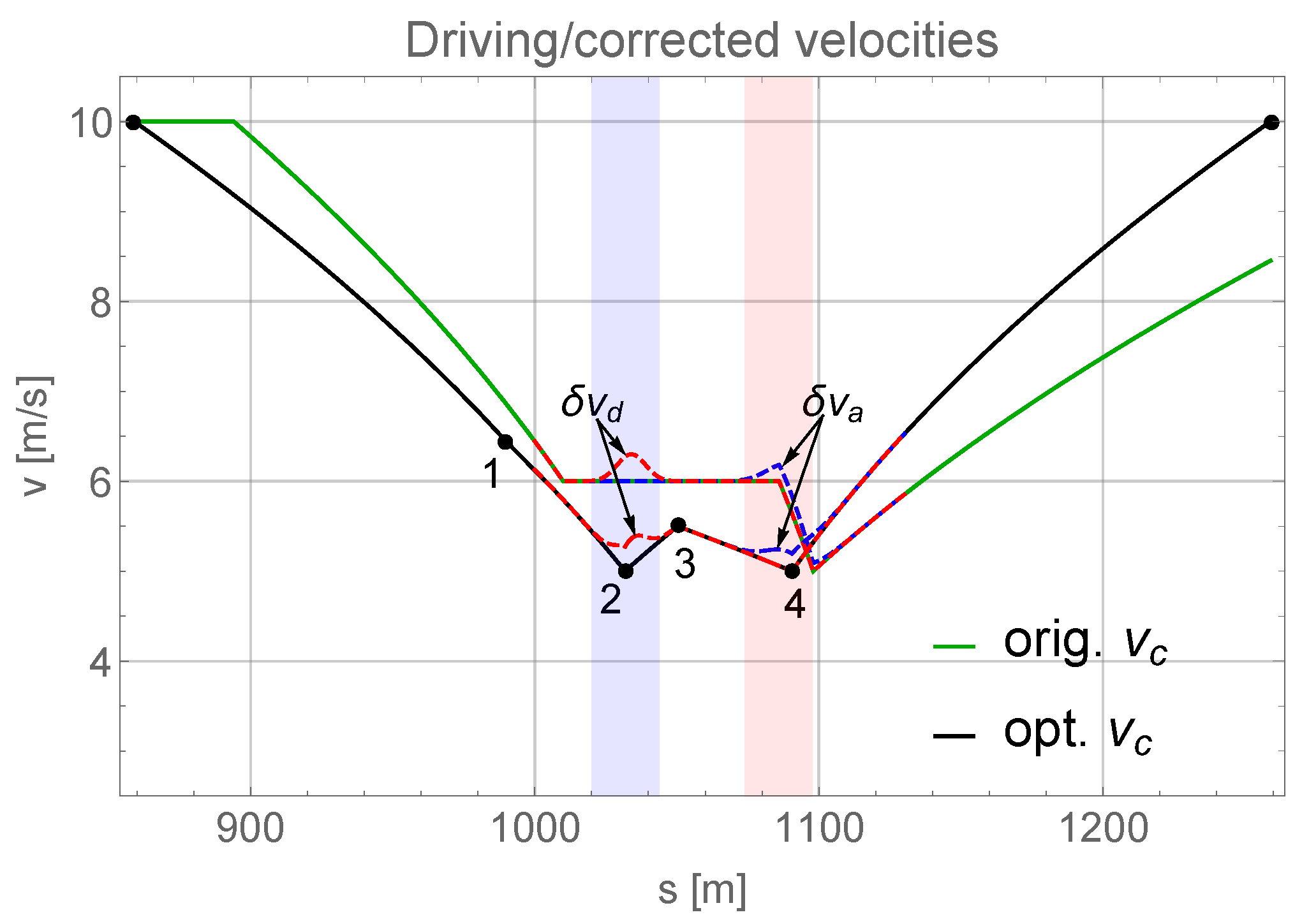
By minimization of J, we obtain the four points ${(S_j,V_j)}_{j=1...4}$ for the optimal velocity within the interval $[s_{min},s_{max}]$, where $s_{max}-s_{min}$ = 400 m, see Figure 3. Since we allowed for variation of the positions of the four points within small regions around the support (ensuring disjunct intervals in position), the run-time was essentially constant and equal to the original run-time. An incorporation of the run-time in the cost function J was therefore not necessary [1]. In order to better approach the measurements in which we used empty vehicles, the minimization of J was executed for the empty vehicles as well. However, it turns out that the solution depends only negligibly on the vehicle mass. This indicates that the obtained optimal velocity profile is rather robust under different loadings (to capture the mass dependency, it is possible to generalize the cost function by summation over many loads).

3. Experimental Validation and Discussion

The experimental setups and methods of velocity, as well as pendulum angle measurements are discussed and presented in detail in our recent work [14]. There, one can find results obtained with the original velocity profile, as well as damping measurements of the static vehicle with different loadings. Here, we use these methods and results to make a comparison with the new, optimized velocity profile. Furthermore, we use here the improved velocity model expressed by Equation (2) to better fit the theory and experiment.

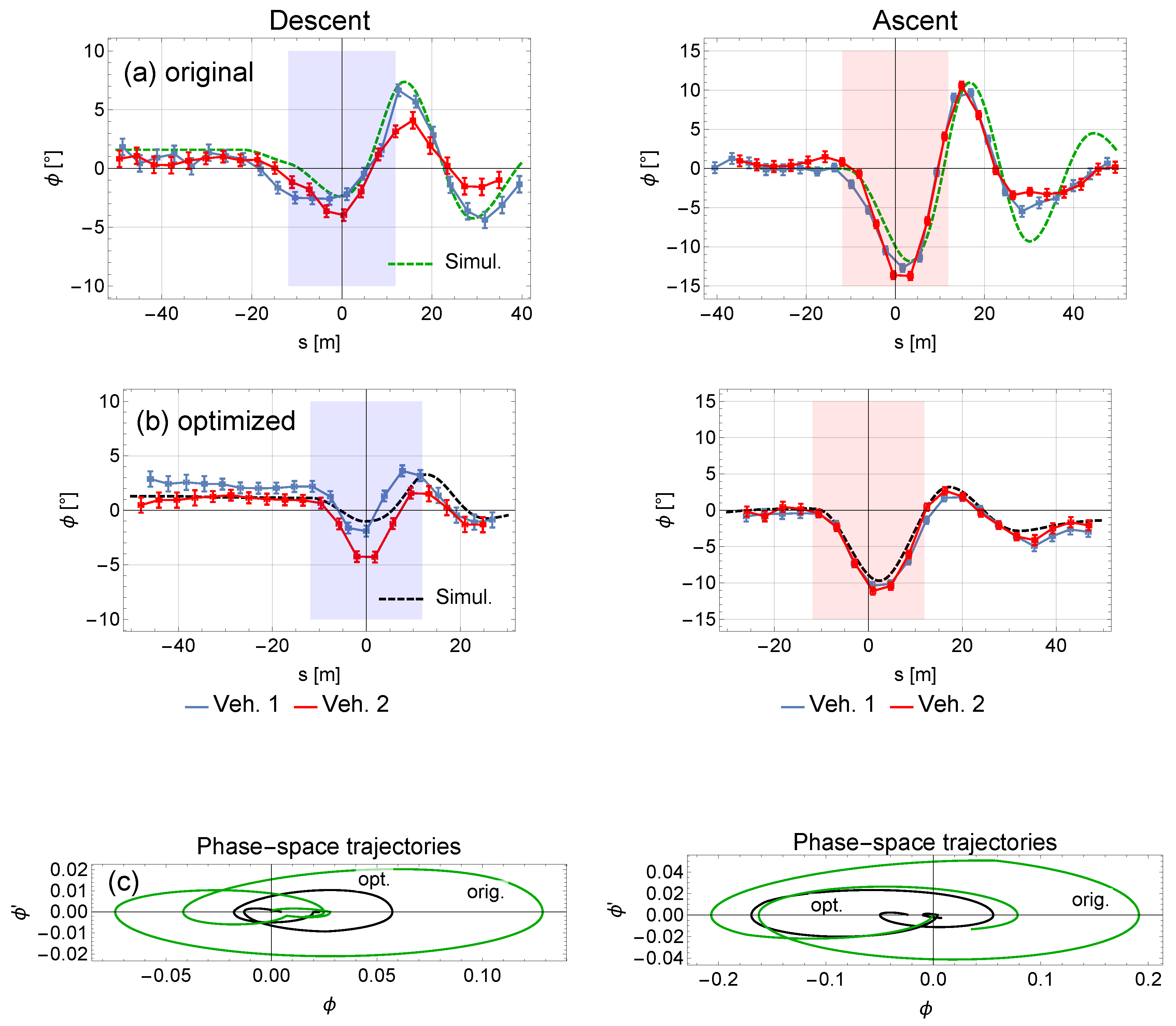
We start the discussion with Figure 2, which shows the measured vehicle velocities (vehicle 1 only, where in the video this is the vehicle in the background) for the descent and ascent case. In order to estimate velocity fluctuations for different rides, we made several measurements, where two of them are plotted for both driving directions. The dashed lines correspond to the theoretical corrected velocities, using the Gaussian modifications according to Equation (2). Figure 3 shows the optimal and the original velocity profile, together with the Gaussian corrections. The four labeled points indicate the solution of the minimization of J. The solution shows a slower speed, compared with the original velocity profile. This is not surprising, because we set the minimal allowed velocity at 5 m/s—more interesting, however, is the position of the points 2 and 4, which are located at the support head. This is also in contrast to any traditional velocity profile, where one simply decelerates before and accelerates after the support passing. Figure 4 contains the results of the video evaluation, the pendulum angles for the original (row (a)), and the optimized velocity profile (row (b)) for both vehicles and both driving directions. The results of simulations are also shown. One can see a difference between the two vehicles in the measurements, in particular for the descending ride in (b), where in the region $s\approx -40$ …−15 m, a constant deceleration along a straight line should result in equal pendulum angles, which indeed is not the case. Since an uncertainty in $v_c$ is certainly not the reason for this difference, we believe that it is caused by a weak blowing wind. The most significant effect of the optimization is visible in the ascending ride. From (a) to (b), we can see that the second swinging is reduced from $\approx {11}^{\circ }$ to $\approx 3^{\circ }$. In panel (c) we plotted the corresponding phase-space trajectories in the most interesting $s-$ parameter region. The trajectories for the optimal velocity profile are contracted to the origin, which also demonstrates the effectiveness of the optimization. In

Table 2. Summary of the experiments/simulations. The * values are the mean of both vehicles. For the ascending ride we measured and calculated a reduction of the oscillation amplitude of $\approx {10}^{\circ }$, which is a significant improvement.

-	J (Empty)	J (Loaded)	$\mathbf{\Delta }\mathit{\phi }$ Descent (Meas.*/simul.) [${}^{\circ }$]	$\mathbf{\Delta }\mathbf{\phi }$ Ascent (Meas. */simul.) [${}^{\circ }$]
original	11.4	14.3	9.5/11.6	23.5/22.8
optimized	3.9	4.0	6.0/4.3	13.0/12.9

, the measured/simulated results for some quantities are summarized. We observe a reduction of the cost function J and the max. amplitude of the vehicle oscillations $\Delta \phi$ for both driving directions, where simulations and measurements coincide better for the ascending ride, since the relative measurement error is smaller.

The values of the pendulum angle depend only weakly on the load, as we confirmed by simulation and observation. This is reported in Figure 5, where we plotted the pendulum angle for the optimal velocity profile and the empty and loaded vehicle. The influence of the vehicle’s mass on the pendulum angle is more relevant for the damping $m_d$ than for the reduced pendulum length $l_p$. We also checked a traditional velocity profile, where the vehicles pass the support with constant velocity of $v_c$ = 5 m/s, augmented by the introduced Gaussian corrections $\delta v_a$, $\delta v_d$. We obtained for the oscillation amplitudes $\Delta \phi =8.4^{\circ }/17.2^{\circ }$ for the descending/ascending rides.

Moreover, we looked at the behavior of the driving engine. Figure 6 shows a monitoring of the torque measured at the motor in the mountain station for the original and the optimized velocity profile. It is interesting that during the passing around the support, the torque is smoother, when the velocity profile is switched from the original to the optimal. This means that the adjustment of the subsystems “driving engine” and “cables plus vehicles” is improved and the energy exchange is reduced.

4. Conclusions

In this paper, we presented a successful implementation of the optimal velocity profile to steer the Postal–Verano ropeway (South Tirol, Italy). The experiments have shown a significant improvement of the vehicle oscillation behavior for both driving directions (ascent and descent) and the validation of the theoretical optimization procedure. In a video accompanying this paper, we show the results by a comparison of the simulated and real system. Apart from the improvement of passenger comfort, we also found a significant smoothing of the torque at the driving engine. Of course, ropeways are a kind of "individual installation" that has to be adapted to the existing conditions (terrain, inclination, wind conditions, etc.). Accordingly, it is not so easy to evaluate a universal method of analysing these structures and related problems. Nevertheless, we believe that the solution strategy adopted here has the potential, if appropriately adapted and refined, to be applied to improve other aerial cableway plants, especially because it does not require changes in the ”hardware”. We think that the method can have a relevant practical impact, even for energy dissipation considerations in ropeways [21].

References

- Wenin, M.; Windisch, A.; Ladurner, S.; Bertotti, M.L.; Modanese, G. Optimal velocity profile for a cable car passing over a support. Eur. J. Mech. A/Solids 2019, 73, 366–372. [Google Scholar] [CrossRef]
- Bryja, D.; Knawa, M. Computational model of an inclined aerial ropeway and numerical method for analyzing nonlinear cable–car interaction. Comput. Struct. 2011, 98, 1895–1905. [Google Scholar] [CrossRef]
- Brownjohn, J.M. Dynamics of an aerial cableway system. Eng. Struct. 1998, 20, 826–836. [Google Scholar] [CrossRef]
- Yi, Z.; Wang, Z.; Zhou, Y.; Stanciulescu, I. Modeling and vibratory characteristics of a mass-carrying cable system with multiple pulley supports in span range. Appl. Math. Model. 2017, 49, 59–68. [Google Scholar] [CrossRef]
- Sofi, A. Nonlinear in-plane vibrations of inclined cables carrying moving oscillators. J. Sound Vib. 2013, 332, 1712–1724. [Google Scholar] [CrossRef]
- Hurel, G.; Laborde, J.; Jézéquel, L. Simulation of the Dynamic Behavior of a Bi-Cable Ropeway with Modal Bases. Top. Modal Anal. Test. 2019, 9, 43–54. [Google Scholar]
- Sofi, A.; Muscolino, G. Dynamic analysis of suspended cables carrying moving oscillators. Int. J. Solids Struct. 2007, 44, 6725–6743. [Google Scholar] [CrossRef] [Green Version]
- Wu, J.S.; Chen, C.C. The dynamic analysis of a suspended cable due to a moving load. Int. J. Numer. Methods Eng. 1989, 28, 2361–2381. [Google Scholar] [CrossRef]
- Arena, A.; Carboni, B.; Angeletti, F.; Babaz, M.; Lacarbonara, W. Ropeway roller batteries dynamics: Modeling, identification, and full-scale validation. Eng. Struct. 2019, 180, 793–808. [Google Scholar] [CrossRef]
- Wang, L.; Rega, G. Modelling and transient planar dynamics of suspended cables with moving mass. Int. J. Solids Struct. 2010, 47, 2733–2744. [Google Scholar] [CrossRef] [Green Version]
- Gattulli, V.; Alaggio, R.; Potenza, F. Analytical prediction and experimental validation for longitudinal control of cable oscillations. Int. J. Non-Linear Mech. 2008, 43, 36–52. [Google Scholar] [CrossRef] [Green Version]
- Petrova, R. Dynamic Analysis of a Chair Ropeway Exposed to Random Wind Loads. FME Trans. 2005, 33, 123–128. [Google Scholar]
- Research, W. NMinimize. [version 12.2.0]. 2014. Available online: https://reference.wolfram.com/language/ref/NMinimize.html (accessed on 8 March 2021).
- Ladurner, S.; Wenin, M.; Reiterer, D.; Bertotti, M.L.; Modanese, G. Experimental Investigation of the dynamics of a ropeway passing over a support. In Engineering Design Applications III; Öchsner, A., Altenbach, H., Eds.; Springer: Berlin/Heidelberg, Germany, 2020. [Google Scholar]
- Wenin, M.; Windisch, A.; Ladurner, S.; Bertotti, M.L.; Modanese, G. Optimization of the Head Geometry for a Cable Car Passing over a Support. In Engineering Design Applications II; Öchsner, A., Altenbach, H., Eds.; Springer: Berlin/Heidelberg, Germany, 2020. [Google Scholar]
- Czitary, E. Seilschwebebahnen (2. Auflage); Springer: Berlin/Heidelberg, Germany, 1962. [Google Scholar]
- Landau, L.D.; Lifschitz, E.M. Lehrbuch der Theoretischen Physik I, Klassische Mechanik (14.Auflage); Verlag Harry Deutsch: Frankfurt am Main, Germany, 2011. [Google Scholar]
- Canale, R. Schwingungen bei Seilbahnen (5. Teil). Int. Seilb. Rundsch. 2010, 6, 24–26. [Google Scholar]
- Volmer, M. Stochastische Schwingungen an Ausgedehnten Seilfeldern und ihre Anwendung zur Spurweitenberechnung an Seilbahnen; Dissertation am Inst. f. Leichtbau und Seilbahntechnik ETH, CH-8092 Zürich, Nr. 13379; 1999. Available online: https://www.research-collection.ethz.ch/handle/20.500.11850/144468 (accessed on 8 March 2021).
- Hoffmann, K. Oscillation Effects of Ropeways Caused by Cross–Wind and Other Influences. FME Trans. 2009, 175, 175–184. [Google Scholar]
- Szlosarek, R.; Yan, C.; Kröger, M.; Nußbaumer, C. Energy efficiency of ropeways: A model-based analysisi. Public Transp. 2019. [Google Scholar] [CrossRef]
Figure 1.
Sketch of the system and some geometrical quantities for the support head. The radius of curvature r has the minimal value at the center of the support. The tangents at the end points of the support head are . The point here indicates the center of the support head. The derivatives are given in units m.
Figure 2.
Measured vehicle velocities (always vehicle 1) for the original velocity profile (solid lines; the (*) means loaded vehicle) and the theoretical velocities used for simulations (dashed lines). The colored bands indicate the support head.
Figure 3.
Original and optimal velocity of the hauling cable at the driving disk and the applied corrections to receive the corresponding velocities at the vehicle positions. The labeled points are the solution of the global optimization procedure, whereas the outside points were left-fixed.
Figure 4.
Experimental results: The row (a) shows the pendulum angle versus position for the original velocity profile. In (b), the same is shown for the optimized velocity profile. The red and blue lines are measured quantities, supported by error bars, indicating the estimated measurement errors. The dashed lines in (a,b) were obtained by simulation. The row (c) shows the simulated phase-space trajectories for both the original and optimized velocities, respectively.
Figure 5.
Pendulum angles for the optimal velocity profile and the two cases: empty and loaded vehicle. Furthermore, the case is shown when the vehicle passes the support with m/s (plus the corrections , ) without any optimization.
Figure 6.
Screenshot of the control window of the computer at the mountain station for both velocity profiles, where (a) gives the original case and (b) the optimized case, respectively. The yellow lines are the velocity profiles, and the lines in cyan give the torque measured at the electrical engine. As one can see in the center of the images, in (a) the torque shows two peaks when the vehicles pass the support, which disappear in (b) (white arrows).