Scenario-Based Stochastic Framework for Optimal Planning of Distribution Systems Including Renewable-Based DG Units

Abstract

Renewable energy-based distributed generators are widely embedded into distribution systems for several economical, technical, and environmental tasks. The main concern related to the renewable-based distributed generators, especially photovoltaic and wind turbine generators, is the continuous variations in their output powers due to variations in solar irradiance and wind speed, which leads to uncertainties in the power system. Therefore, the uncertainties of these resources should be considered for feasible planning. The main innovation of this paper is that it proposes an efficient stochastic framework for the optimal planning of distribution systems with optimal inclusion of renewable-based distributed generators, considering the uncertainties of load demands and the output powers of the distributed generators. The proposed stochastic framework depends upon the scenario-based method for modeling the uncertainties in distribution systems. In this framework, a multi-objective function is considered for optimal planning, including minimization of the expected total power loss, the total system voltage deviation, the total cost, and the total emissions, in addition to enhancing the expected total voltage stability. A novel efficient technique known as the Equilibrium Optimizer (EO) is actualized to appoint the ratings and locations of renewable-based distributed generators. The effectiveness of the proposed strategy is applied on an IEEE 69-bus network and a 94-bus practical distribution system situated in Portugal. The simulations verify the feasibility of the framework for optimal power planning. Additionally, the results show that the optimal integration of the photovoltaic and wind turbine generators using the proposed method leads to a reduction in the expected power losses, voltage deviations, cost, and emission rate and enhances the voltage stability by 60.95%, 37.09%, 2.91%, 70.66%, and 48.73%, respectively, in the 69-bus system, while in the 94-bus system these values are enhanced to be 48.38%, 39.73%, 57.06%, 76.42%, and 11.99%, respectively.

1. Introduction

1.1. Problem Statement

Uncertainty is essential in the optimal power planning problem of electrical systems, and it is a main consideration adding to its complexity, specifically the uncertainties of the renewable energy resources (RERs) and load demands. Many research efforts related to the optimal integration of Distributed Generators (DGs) are expressed as ideal optimization problems, and only few have considered uncertainty. The optimal allocation of the photovoltaic (PV) and wind turbine (WT) units in power systems and techniques existing in the literature considering the uncertainty of systems have an incredible impact on the planning of renewable DGs, and uncertainties effect the load demand and the output powers of solar and wind-based DGs in the distribution systems (DSs). The contribution and the research gap are referenced in detail. Electric power generation organizations will in general utilize (DGs) near the load to convey the electrical power to the consumers for technical, economic, and environmental reasons. As of late, integration of the RERs including wind and photovoltaic energies have become a favored solution for defeat increasing the load growth as they are sustainable and clean resources. Nonetheless, the inclusion of the RERs in the distribution grids face numerous issues due to their intermittency and the fluctuations of the output power, which increases the uncertainties in electrical systems. In this way, the uncertainties in power systems should be taken into consideration for correct planning and the secure operation of power systems.

1.2. Literature Survey

The essential purpose of efficient planning in distribution systems is to provide excellent solutions that guarantee the security, quality, and reliability of power supply to clients at the least cost [1]. The cost of power generation from conventional generators is expanding quickly because of the increase in fuel costs, although lately the generation cost of RERs has diminished. Alongside financial contemplations, another advantage of RERs is the eco-friendly power generation from these sources [2]. A stochastic scenario modeling of a multistage joint for the distribution systems planning has been utilized to decrease the operational and investment costs [3]. Sensible application of DGs can bring numerous points of interest, for example, voltage profile improvement, reducing emissions and energy cost [4,5,6].

Nonetheless, improper placement of DGs may lead to the fluctuations of voltage and also system instability because of the uncertain nature of RERs [7,8]. The issue of optimal integration of DGs has been explored in the several papers from different points of view. The authors in [9] suggested an improved adaptive genetic algorithm for resolving the optimal DG allocation problem. In [10], an efficient framework has been suggested for the optimal DG allocation problem to reduce the system costs. The authors in [11] offered a genetic algorithm along with the Monte Carlo method for solving the optimal DG integration problem under the uncertainties of RER generation. The cost of energy losses and DGs have been considered in the model. In [12], an efficient method has been presented for the optimal planning of accommodating the integration of PEV along with renewable DGs under uncertainties of the system. In [13], the optimal power planning problem in the active distribution system is solved to reduce total cost and emissions using a cuckoo search (CS) with optimal integration of WTs and demand response, considering the uncertainties of the system by the scenario synthesis method. The authors in [14] applied the Crisscross Optimization Algorithm and Monte Carlo Simulation for assigning the rating and location of DGs in the distribution system for reducing the power losses and the cost. Esmaeili et al. presented a multi-objective framework for optimizing the DG allocation and reconfiguration of the distribution network using the Big Bang–Big Crunch algorithm [15]. In [16], a probabilistic planning method was suggested based on mixed integer nonlinear programming (MINLP) and has been implemented to assign energy loss reduction with optimal integration of RERs in a rural distribution system. The author in [17] proposed a stochastic model for optimizing the investment of the DGs under uncertain conditions in distribution networks. Ref. [18] proposed a planning strategy for a hybrid solar-wind generation MG system with hydrogen energy storage using a novel multi-objective optimization algorithm to minimize the following three objective functions: loss of load expected, annualized cost of the system, and loss of energy expected. Ref. [19] proposed an algorithm for DG allocation planning based on using the probabilistic uncertainty modeling method. Several optimization algorithms have been used to determine the best size and location of DGs in a radial distribution network (RDN) considering the uncertainties of systems such as Particle Swarm Optimization (PSO) [20], modified sine cosine algorithm [21], Cuckoo Search Algorithm (CA) [22], water cycle algorithm [23], Improved Antlion Optimization Algorithm (IALO) [24], Specialized Genetic Algorithm (SGA) [25], Ant Colony Optimizer (ACO) [26], Modified Differential Evolution Algorithm (MDEA) [27], harmony search algorithm [28], Seeker Optimization Algorithm (SOA) [29], and teaching learning-based optimization [30].

The Equilibrium Optimizer (EO) is a novel physical-based optimization technique which emulates the control volume mass balance models [31]. The EO has been applied for solving numerous engineering problems, and in [32] it has been applied for solving the economic dispatch of a micro-grid The authors in [33] applied the EO for assigning the optimal rating and locations of the renewable-based DGs for loss reduction under uncertainties of the system. In [34], the EO was implemented for optimizing the structural design of vehicle components. The EO was employed for solving the optimal power flow problem in an AC/DC network. The solar photovoltaic parameters have been estimated using the EO in [35].

In this paper, the EO is utilized for deciding the best allocation of the solar and wind units for minimization of the expected power losses, the system voltage deviation, the total cost, and the total emissions as well as enhancing the expected voltage stability considering the uncertainties of load demands and solar and wind power generators in an IEEE 69-bus network and a 94-bus practical distribution system situated in Portugal.

1.3. Contribution of Paper

From the previous survey, the main concern or the problem statement related to the optimal planning of distribution systems with the inclusion of optimal RERs is the uncertainties of load demand and the output power of the RERs. Therefore, the planning problem became more complex and needs an efficient method to be solved.

This paper contributes to the existing body of knowledge as it solves the optimal planning problem in a distribution system for optimal incorporation of DGs using a scenario-based stochastic framework considering the uncertainties of load demands and the output powers of RERs. The innovation and contributions of this paper are summarized as follows:

• Proposing an efficient framework for the optimal planning of distribution systems considering the uncertainties of load and the output powers of renewable based DGs.
• The application of scenario-based methods for modeling the uncertainties in the electrical systems.
• The application of an efficient algorithm, called the EO, for solving the planning problem.
• The developed algorithms are applied for optimal integration of the renewable-based DGs for loss reduction, voltage improvements, system voltage deviation, the total cost, and the total emissions of the IEEE 69-bus and 94-bus distribution networks.
• A comparison is presented between the EO and other well know techniques for solving the planning problem.

1.4. Paper Layout

The paper is arranged as follows: Section 2 displays the problem formulation including the objective function. Section 3 illustrates the uncertainty modeling methods. Section 4 introduces an overview of the EO technique. Section 5 shows the obtained outcomes, while Section 6 lists the paper’s conclusions.

2. Problem Formulation

In this study, five objective functions are considered in a multi-objective function. It is worth mentioning that in case of modeling or considering the uncertainties in power systems, a set of scenarios will be generated. Thus, these scenarios should be considered for the efficient solving of planning problems, and each scenario has its expected values as depicted in the following sections. In this work, the considered objective function is a multi-objective function comprising five objective functions which can be presented as follows:

2.1. The Objective Functions

2.1.1. Minimization of the Expected Power Loss ($E{P}_{Loss}$)

The expected power losses of the radial distribution network are determined as follows:

$$P_{loss}{}_{\left(k,k+1\right)}=R_{k,k+1}\left(\frac{P_k^2+j{Q}_k^2}{{\left|V_k\right|}^2}\right)$$

(1)

where

$$P_{Total\_Loss}={\displaystyle \sum }_{i=1}^{NT}{P}_{Loss,i}$$

(2)

$$ET{P}_{Loss}={\displaystyle \sum }_{k=1}^{Ns}E{P}_{Loss,k}={\displaystyle \sum }_{k=1}^{Ns}{\pi }_{S,k}\times P_{Tota{l}_{Loss},k}$$

(3)

2.1.2. Minimization of the Expected Voltage Deviations ($ETVD$)

The expected summation of the voltage deviations of the radial distribution network are given as follows:

$$ETVD={\displaystyle \sum }_{k=1}^{Ns}EV{D}_k={\displaystyle \sum }_{k=1}^{Ns}{\pi }_{S,k}\times V{D}_k$$

(4)

where

$$VD={\displaystyle \sum }_{n=1}^{NB}\left|V_n-1\right|$$

(5)

2.1.3. Enhancement of the Expected Voltage Stability ($ETVSI$)

The expected summation of the voltage stability indices can be expressed as follows:

$$ETVSI={\displaystyle \sum }_{k=1}^{Ns}EVS{I}_k={\displaystyle \sum }_{k=1}^{Ns}{\pi }_{S,k}\times VS{I}_k$$

(6)

where

$$VS{I}_n={\left|V_n\right|}^4-4{\left(P_n{X}_{nm}-Q_n{R}_{nm}\right)}^2-4\left(P_n{X}_{nm}+Q_n{R}_{nm}\right){\left|V_n\right|}^2$$

(7)

2.1.4. Minimization of the Expected Total Cost ($ETCost$)

The expected total annual cost ($ETCost$) is considered, which consists of the expected annual energy loss cost ($ECos{t}_{loss}$), the expected cost of the electric energy savings from the main substation ($ECos{t}_{Grid}$), the expected PV units cost ($ECos{t}_{PV}$), and the expected WT cost ($ECos{t}_{WT}$). It can be represented as follows:

$$ETCost=ECos{t}_{loss}+ECos{t}_{Grid}+ECos{t}_{PV}+ECos{t}_{WT}$$

(8)

The items detailed in Equation (8) are defined as follows:

$$Cos{t}_{Grid}=8760\times K_{Grid}\times P_{Grid}$$

(9)

$$ETCos{t}_{Grid}={\displaystyle \sum }_{k=1}^{Ns}ECos{t}_{Grid,k}={\displaystyle \sum }_{k=1}^{Ns}{\pi }_{S,k}\times Cos{t}_{Grid,k}$$

(10)

$$Cos{t}_{Loss}=8760\times K_{Loss}\times P_{Total\_loss}$$

(11)

$$ETCos{t}_{Loss}={\displaystyle \sum }_{k=1}^{Ns}ECos{t}_{Loss,k}={\displaystyle \sum }_{k=1}^{Ns}{\pi }_{S,k}\times Cos{t}_{Loss,k}$$

(12)

$$ETCos{t}_{wind}={\displaystyle \sum }_{k=1}^{Ns}ECos{t}_{wind,k}={\displaystyle \sum }_{k=1}^{Ns}{\pi }_{S,k}\times \left(a_1+8760\times b_1\times P_{WT,k}\right)$$

(13)

$$a_1=CF\times CSD{G}_{WT}\times P_{wr}$$

(14)

$$b_1=Cost\_W{T}_{O\&M}+Cost\_W{T}_{Fuel}$$

(15)

$$CF=\frac{\rho \times {\left(1+\rho \right)}^{NP }}{{\left(1+\rho \right)}^{NP}-1}$$

(16)

where $a_1$ is the annual installment of the wind turbine, and $b_1$ is the annual operation and maintenance cost of the wind turbine.

$$ETCos{t}_{PV}={\displaystyle \sum }_{k=1}^{Ns}ECos{t}_{PV,k}={\displaystyle \sum }_{n=1}^{Ns}{\pi }_{S,k}\times \left(a_2+8760\times b_2\times P_{PV,k}\right)$$

(17)

$$a_2=CF\times CSD{G}_{PV}\times P_{sr}$$

(18)

$$b_2=Cost\_P{V}_{O\&M}+Cost\_P{V}_{Fuel}$$

(19)

where $a_2$ is the annual installment of the PV unit, and $b_2$ is the annual operation and maintenance cost of the PV unit. In this paper the cost coefficients of PV are selected to be $CSD{G}_{PV}=770$ USD/kW, $Cost\_P{V}_{O\&M}=0.01$ USD/kWh, $Cost\_P{V}_{Fuel}=0$ USD/kWh, and the cost coefficients of the wind are selected to be $CSD{G}_{WT}=4000$ USD/kW, $Cost\_W{T}_{O\&M}=0.01$ USD/kWh, $Cost\_W{T}_{Fuel}=0$ USD/kWh [36].

2.1.5. Minimization of the Expected Total Emissions ($ETEmission$)

The expected total annual emissions in kilotons (Kt) can be expressed as follows:

$$ETEmission={\displaystyle \sum }_{k=1}^{Ns}EEmissio{n}_k={\displaystyle \sum }_{n=1}^{Ns}{\pi }_{S,k}\times P_{Grid,k}\times LF\times E{R}_{Grid}\times 8760$$

(20)

According to $E{R}_{Grid}$, the emission rate of grid values of NOx, CO_2, and SO₂ are 2.2952 kg/MWh, 921.25 kg/MWh and 3.5834 kg/MWh, respectively [15].

2.1.6. The Multi-Objective Function

In this work, the previous objective functions are considered simultaneously. To consider these objective functions concurrently, the weight approach method is utilized. In addition, the objectives should be normalized as follows via division by its base value (without PV or WT), which makes the objective function dimensionless and also prevents any scaling problems. The augmented objective function can be described as follows:

$$F={\propto }_1{F}_1+{\propto }_2{F}_2+{\propto }_3{F}_3+{\propto }_4{F}_4+{\propto }_5{F}_5$$

(21)

where ${\propto }_1$, ${\propto }_2$, ${\propto }_3$, ${\propto }_4$, and ${\propto }_5$ are weighting factors. The summation of weight factors should equal 1 as follows:

$$\left|{\propto }_1\right|+\left|{\propto }_2\right|+\left|{\propto }_3\right|+\left|{\propto }_4\right|+\left|{\propto }_5\right|=1$$

(22)

The normalized objective functions can be formulated as follows:

$$F_1=\frac{ET{P}_{Loss}}{ET{P}_{Los{s}_{base}}}$$

(23)

$$F_3=\frac{ETVD}{ETV{D}_{base}}$$

(24)

$$F_3=\frac{1}{ETVSI}$$

(25)

$$F_4=\frac{ETCost}{ETCos{t}_{base}}$$

(26)

$$F_5=\frac{ETEmission}{ETEmissio{n}_{base}}$$

(27)

2.2. The System Constraints

The system constraints are categorized as follows:

2.2.1. Equality Constraints

$$P_{Grid}+{\displaystyle \sum }_{i=1}^{NPV}{P}_{PV,i}+{\displaystyle \sum }_{i=1}^{NWT}{P}_{WT,i}={\displaystyle \sum }_{i=1}^{NT}{P}_{loss,i}+{\displaystyle \sum }_{i=1}^{NB}{P}_{L,i}$$

(28)

$$Q_{Grid}+{\displaystyle \sum }_{i=1}^{NT}{Q}_{WT,i}={\displaystyle \sum }_{i=1}^{NT}{Q}_{loss,i}+{\displaystyle \sum }_{i=1}^{NB}{Q}_{L,i}$$

(29)

2.2.2. Inequality Constraints

$$V_{min}\le V_i\le V_{max}$$

(30)

$${\displaystyle \sum }_{i=1}^{NWT}{Q}_{WT,i}\le {\displaystyle \sum }_{i=1}^{NB}{Q}_{L,i}$$

(31)

$$I_n\le I_{max,n} n=1,2,3\dots ,NT$$

(32)

3. Uncertainty Modeling

In this work, the uncertainties that existed in the power system are considered by solving the problem of optimal power planning. The proposed stochastic framework considered three uncertain parameters including load demand, solar irradiance, and wind speed. The continuous probability density functions (PDFs) of wind speed, solar irradiance, and loads are used for representing the uncertainties of these parameters; then, the scenario-based method is utilized for generating a set of scenarios from combinations of these parameters. The proposed stochastic framework can be depicted as follows:

3.1. Modeling of Load Demand

The normal PDF ($f_d\left(P_d\right)$) is used for uncertainty representation of the load demand, which can be described using the following equations [37]:

$$f_d\left(P_d\right)=\frac{1}{{\sigma }_d\sqrt{2\pi }}exp\left[-\frac{{\left(P_d-{\mu }_d\right)}^2}{2{\sigma }_d{}^2}\right]$$

(33)

The generated load scenarios and their probabilities obtained from (33) can be obtained as follows [38]:

$${\pi }_{d,i}={{\displaystyle \int }}_{P_{d,i}^{min}}^{P_{d,i}^{max}}\frac{1}{{\sigma }_d\sqrt{2\pi }}exp\left[-\frac{{\left(P_d-{\mu }_d\right)}^2}{2{\sigma }_d{}^2}\right]d{P}_d$$

(34)

$$P_{d,i}=\frac{1}{{\tau }_{d,i}}{{\displaystyle \int }}_{P_{d,i}^{min}}^{P_{d,i}^{max}}\frac{P_d}{{\sigma }_d\sqrt{2\pi }}exp\left[-\frac{{\left(P_d-{\mu }_d\right)}^2}{2{\sigma }_d{}^2}\right]d{P}_d$$

(35)

In this work, three load scenarios are presented. The load scenarios are obtained by dividing the normal PDF into three intervals.

Table 1. The generated scenarios of the uncertain parameters.

Load Scenario	${\mathit{\pi }}_{\mathit{d},\mathit{i}}$	Loading %
1	0.1587	54.7486
2	0.6827	70.0000
3	0.1587	85.2514
Wind Scenario	${\pi }_{wind,z}$	Wind Speed (m/s)
1	0.7902	7.4518
2	0.1694	13.6153
3	0.0404	17.7289
Irradiance Scenario	${\pi }_{Solar,m}$	Solar Irradiance (W/m2)
1	0.1605	416.0627
2	0.4412	609.1166
3	0.3983	790.4621

provides the load scenarios and their probabilities when ${\mu }_d$ and ${\sigma }_d$ are 70 and 10 [39].

3.2. Modeling of Wind Speed

The Weibull PDFs ($f_v\left(v\right)$) are used to describe the uncertainties of wind speed which can be expressed as follows [38]:

$$f_v\left(v\right)=\left(\frac{k}{c}\right){\left(\frac{k}{c}\right)}^{\left(k-1\right)}{e}^{-{(v/c)}^k}\hspace{1em}0\le v<\infty$$

(36)

The wind turbine output power can be specified as follows [40,41]:

$$P_w\left(v_{\omega }\right)=\{\begin{array}{ccc}0& for& v_{\omega }<v_{\omega i} \& v_{\omega }>v_{\omega o}\\ P_{wr}\left(\frac{v_{\omega o}-v_{\omega i}}{v_{\omega r}-v_{\omega i}}\right)& for& \left(v_{\omega i}\le v_{\omega }\le v_{\omega r}\right)\\ P_{wr}& for & \left(v_{\omega r}<v_{\omega }\le v_{\omega o}\right)\end{array}$$

(37)

Additionally, a set of scenarios can be obtained from (36) by dividing the $f_v\left(v\right)$ into of a set of wind speed intervals. The generated wind speeds and their probabilities can be obtained as follows [42]:

$${\pi }_{wind,z}={{\displaystyle \int }}_{v_z^{min}}^{v_z^{max}}\left(\left(\frac{k}{c}\right){\left(\frac{k}{c}\right)}^{\left(k-1\right)}{e}^{-{(v/c)}^z}\right)dv$$

(38)

$$v_z=\frac{1}{{\pi }_{wind,z}}{{\displaystyle \int }}_{v_z^{min}}^{v_z^{max}}\left(\left(\frac{k}{c}\right){\left(\frac{k}{c}\right)}^{\left(z-1\right)}{e}^{-{(v/c)}^z}\right)dv$$

(39)

In this paper, three scenarios of wind speed are generated from the previous equations. The wind speed scenarios and their probabilities are listed in Table 1 in the case of selecting $c$ and $k$ to be 10.0434 and 2.5034, respectively, as given in [38].

3.3. Modeling of Solar Irradiance

The Beta PDF is used to specify the uncertainty of the solar irradiance, which can be given as follows [43]:

$$f_G\left(G\right)=\{\begin{array}{c}\frac{\mathrm{\Gamma }\left(\alpha +\beta \right)}{\mathrm{\Gamma }\left(\alpha \right)+\mathrm{\Gamma }\left(\beta \right)}\times G^{\propto -1}\\ \times {\left(1-G\right)}^{\beta -1}\\ 0otherwise\end{array} If 0\le G\le 1, 0\le \alpha ,\beta$$

(40)

$$\beta =\left(1-{\mu }_s\right)\times \left(\frac{{\mu }_s\times \left(1+{\mu }_s\right)}{{{\sigma }_s}^2}\right)-1$$

(41)

$${\sigma }_s=\left(1-{\mu }_s\right)\times \left(\frac{{\mu }_s\times \beta }{\left(1-{\mu }_s\right)}\right)-1$$

(42)

The yield power from the PV system can be calculated as follows [44,45]:

$$P_s\left(G\right)=\{\begin{array}{c}{P}_{sr}\left(\frac{G^2}{G_{std}\times X_c}\right) for 0<G\le X_c\\ P_{sr}\left(\frac{G}{G_{std}}\right) for G\ge X_c\end{array}$$

(43)

In the previous equation, $G_{std}$ is set to be 1000 $\mathrm{W}/{\mathrm{m}}^2$, and $X_c$ is a certain irradiance point is set to be 120 $\mathrm{W}/{\mathrm{m}}^2$ [41]. Three scenarios can be obtained from the previous equations by dividing the PDF into three intervals. The portability of solar irradiance and its corresponding solar irradiance for each scenario are given as follows [42]:

$${\pi }_{Solar,m}={{\displaystyle \int }}_{G_m^{min}}^{G_m^{max}}{f}_G\left(G\right)dG$$

(44)

$$G_m=\frac{1}{{\pi }_{Solar,m}}{{\displaystyle \int }}_{G_m^{min}}^{G_m^{min}}\left(\frac{\Gamma \left(\alpha +\beta \right)}{\Gamma \left(\alpha \right)·\Gamma \left(\beta \right)}\times \left(G^{\propto -1}\right)\times {\left(1-G\right)}^{\beta -1}\right)dG$$

(45)

The generated scenarios of the solar irradiance and their probabilities are listed in Table 1 in the case of selecting $\alpha$ and $\beta$ to be 6.38 and 3.43, respectively, as given in [38].

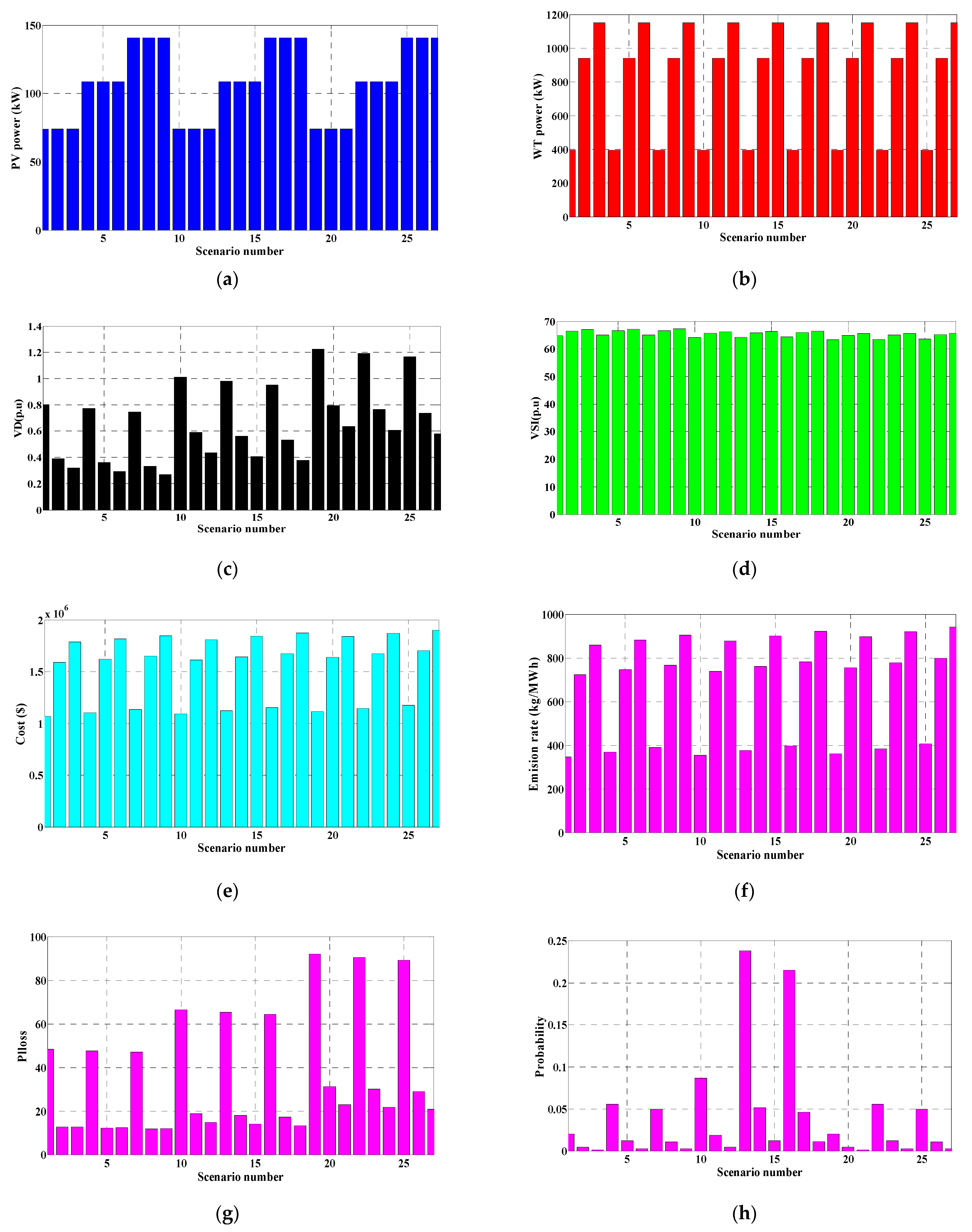
3.4. The Combined Load-Generation Model

To consider the uncertainties of the load demand, wind speed, and irradiance simultaneously, the probabilities of these parameters depicted in (34), (38), and (44) are multiplied together according to (46) as follows:

$${\pi }_S={\pi }_{d,i}\times {\pi }_{wind,k}\times {\pi }_{Solar,m}$$

(46)

A total of 27 scenarios can be obtained from (46).

Table 2. The combined scenarios and their probabilities.

Scenario	Loading %	Wind Speed (m/s)	Solar Irradiance (W/m2)	${\mathit{\pi }}_{\mathit{d},\mathit{i}}$	${\mathit{\pi }}_{\mathit{Solar},\mathit{m}}$	${\mathit{\pi }}_{\mathit{wind},\mathit{z}}$	${\mathit{\pi }}_{\mathit{S}}$
$\mathrm{S}1$	54.7486	7.4518	416.0627	0.1587	0.1605	0.7902	0.0201
$\mathrm{S}2$	54.7486	13.6153	416.0627	0.1587	0.1605	0.1694	0.0043
$\mathrm{S}3$	54.7486	17.7289	416.0627	0.1587	0.1605	0.0404	0.0010
$\mathrm{S}4$	54.7486	7.4518	609.1166	0.1587	0.4412	0.7902	0.0553
$\mathrm{S}5$	54.7486	13.6153	609.1166	0.1587	0.4412	0.1694	0.0119
$\mathrm{S}6$	54.7486	17.7289	609.1166	0.1587	0.4412	0.0404	0.0028
$\mathrm{S}7$	54.7486	7.4518	790.4621	0.1587	0.3983	0.7902	0.0499
$\mathrm{S}8$	54.7486	13.6153	790.4621	0.1587	0.3983	0.1694	0.0107
$\mathrm{S}9$	54.7486	17.7289	790.4621	0.1587	0.3983	0.0404	0.0026
$\mathrm{S}10$	70.0000	7.4518	416.0627	0.6827	0.1605	0.7902	0.0866
$\mathrm{S}11$	70.0000	13.6153	416.0627	0.6827	0.1605	0.1694	0.0186
$\mathrm{S}12$	70.0000	17.7289	416.0627	0.6827	0.1605	0.0404	0.0044
$\mathrm{S}13$	70.0000	7.4518	609.1166	0.6827	0.4412	0.7902	0.2380
$\mathrm{S}14$	70.0000	13.6153	609.1166	0.6827	0.4412	0.1694	0.0510
$\mathrm{S}15$	70.0000	17.7289	609.1166	0.6827	0.4412	0.0404	0.0122
$\mathrm{S}16$	70.0000	7.4518	790.4621	0.6827	0.3983	0.7902	0.2149
$\mathrm{S}17$	70.0000	13.6153	790.4621	0.6827	0.3983	0.1694	0.0461
$\mathrm{S}18$	70.0000	17.7289	790.4621	0.6827	0.3983	0.0404	0.0110
$\mathrm{S}19$	85.2514	7.4518	416.0627	0.1587	0.1605	0.7902	0.0201
$\mathrm{S}20$	85.2514	13.6153	416.0627	0.1587	0.1605	0.1694	0.0043
$\mathrm{S}21$	85.2514	17.7289	416.0627	0.1587	0.1605	0.0404	0.0010
$\mathrm{S}22$	85.2514	7.4518	609.1166	0.1587	0.4412	0.7902	0.0553
$\mathrm{S}23$	85.2514	13.6153	609.1166	0.1587	0.4412	0.1694	0.0119
$\mathrm{S}24$	85.2514	17.7289	609.1166	0.1587	0.4412	0.0404	0.0028
$\mathrm{S}25$	85.2514	7.4518	790.4621	0.1587	0.3983	0.7902	0.0499
$\mathrm{S}26$	85.2514	13.6153	790.4621	0.1587	0.3983	0.1694	0.0107
$\mathrm{S}27$	85.2514	17.7289	790.4621	0.1587	0.3983	0.0404	0.0026

shows the obtained scenarios and the value of the uncertain parameters and their probabilities.

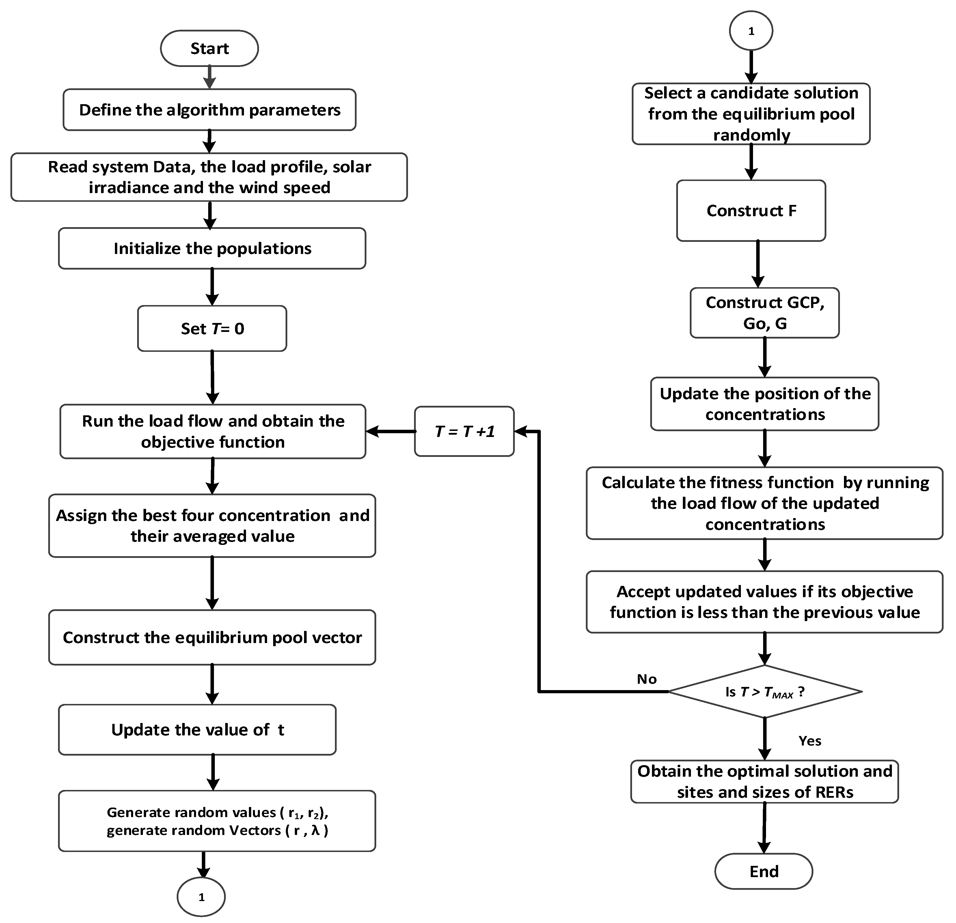
4. Equilibrium Optimizer

The EO is a modern optimizer which simulates models of the control volume mass balance to describe the dynamic and equilibrium states. In the EO, the concentrations denote the positions or the locations, while the particles represent the search agents of the optimizer. The particles update their location randomly around a vector known as equilibrium candidates. In addition, the generation rate is utilized for boosting the exploration and exploitation of the optimizer [31]. The mass balanced equation is described according to Equation (47) as follows:

$$V\frac{dX}{dt}=D{X}_{eq}-QX+G$$

(47)

where $V\frac{dX}{dt}$ describes the rate of mass changing in a volume. $X$ refers to the concentration, and $V$ represents the control volume. $Q$ denotes the flow rate. $G$ denotes the mass generation rate. By integration and manipulation of Equation (47), it is formulated as follows:

$$X=X_{eq}+\left(C_0-C_{eq}\right)exp\left[-\lambda \left(t-t_0\right)\right]+\frac{G}{\lambda V} \left(1-\left(exp\left[-\lambda \left(t-t_0\right)\right]\right)\right)$$

(48)

where $\lambda =\left(\frac{D}{V}\right).$ $X_0$ refers to the initial concentration, and $t_0$ is the initial start time.

The Steps of EO

Step 1: Initialization

The initial concentrations are generated randomly according to (49).

$$X_i^{initial}=X_{min}+ran{d}_i (X_{max}-X_{min}) i=1,2,\dots \dots n$$

(49)

where $X_{max}$ is the upper boundary of the control variable, while $X_{min}$ is its lower limit.

$rand$ is a random value in the range [0,1]. Then, the objective function is evaluated for each obtained concentration.

Step 2: Assignment of the Equilibrium Candidates

The concentrations will be sorted according to their objective functions. The best four concentrations and their average vector represent the equilibrium candidates or the pool vector ($X_{pool}$), which can be expressed using (50) the following:

$$X_{pool}=\left\{X_1,X_2 ,X_3,X_4, X_{avg}\right\}$$

(50)

where

$$X_{avg}=\frac{X_1+X_2+X_3+X_4}{4}$$

(51)

Step 3: Updating of the concentrations

Two vectors (r, $\lambda$) are created randomly, and they are used to control the exponential factor (F) to update the concentrations according to the following equations:

$$F=L_{1}sign\left(r-0.5\right)\left[e^{-\lambda t}-1\right]$$

(52)

where

$$t={\left(1-\frac{T}{T_{Max}}\right)}^{(L_2 \frac{T}{T_{Max}})}$$

(53)

where $L_1$ and $L_2$ are constant values, which equal 2 and 1, respectively. These values are employed to adjust the exponential factor. $T_{Max}$ is the maximum number of iterations, $T$ refers to the T-th iteration. It should be indicated here that $a_1$ is employed to control the exploration process, while $a_2$ is employed to control the exploitation phase o. Sign (r − 0.5) can also control the exploration direction.

Step 4: Applying the generation rate

It worth mentioning here that the generation rate is a robust approach for exploitation enhancement, and it can be defined as follows:

$$G=G_0 e^{-k\left(t-t_0\right)}$$

(54)

where

$$G_0=GCP \left(X_{pool}-\lambda X\right)$$

(55)

$$GCP=\{\begin{array}{c}0.5 r_1{r}_2\ge GP\\ 0 r_2<GP\end{array}$$

(56)

where $r_1$ and $r_2$ refer to a random value in the range of [0,1]. $GP$ is the probability of generation, which is utilized to control the participation probability of concentration where it is updated by the generation rate. When $GP$ = 1, the generation rate will not participate in the optimization process, while when $GP$ = 0, the generation rate will greatly participate in the process. If $GP=0$, the generation rate offers an admirable balancing between the exploration and exploitation procedures. According to the mentioned steps, the updated equation can be described using Equation (57):

$$X=X_{pool}+\left(X-X_{pool}\right)·F+\frac{G}{\lambda V}\left(1-F\right)$$

(57)

Step 5: Adding memory saving.

The obtained solutions or concentration will be compared with the previous solution. It is worth mentioning here that the EO is proposed to solve the presented optimal planning problem, where the main advantages of the Equilibrium Optimizer lie in its ability to assign optimal solutions with higher efficiency (i.e., less computational time or fewer number of iterations) when compared with other optimization techniques, as well as its high simplicity in updating the algorithm structure and its controllability between the exploitation and exploration phases. Its related disadvantage is that it is very sensitive to its selected parameters. Figure 1 describes application of the EO for the solution of the optimal power planning problem.

5. Results and Discussion

The optimal power planning problem has been solved by the suggested algorithm (EO), and the optimal ratings and placement of wind turbines and solar PV units are assigned under the uncertainties of renewable energy and load demand. The objective function is a multi-objective function which comprises of (1) the expected power loss, (2) the expected summation of voltage deviations, (3) the expected voltage stability index, (4) the expected cost, and (5) the expected emissions. It should be highlighted here that the value of each weight factors in (21) is selected to be 0.2 for all studied cases. The EO algorithm is implemented for IEEE 69 and 94-bus systems, and the outcomes are compared with those obtained by the Sine Cosine Algorithm (SCA) [46], Particle Swarm Optimizer (PSO) [47], and the Anti Lion Algorithm (ALO) [48]. The single line diagram of the IEEE 69 and 94-bus systems are illustrated in Figure 2 and Figure 3, respectively. The systems data of the 69-bus and 94-bus systems are given in [49,50], respectively. The system data and the initial load flow are provided in

Table 3. The specifications of the studied systems and initial load flow solutions.

Item	69-Bus	94-Bus
System voltage	12.66 KV	15KV
$V_{min}$ (p.u)	0.90919 @ bus 65	0.84749 @ bus 92
$V_{max}$ (p.u) excluding the slack bus	0.99997 @ bus 2	0.99508 @ bus 2
Total active load demand (KW)	3801.490	4797.000
Total reactive load demand (KVAR)	2694.600	2323.900
Total active loss (KW)	224.975	365.173
Total reactive loss (KVAR)	102.187	505.785

, while the constraints of the system are given in

Table 4. The system constraints.

Parameter	Value
Voltage limits	$0.90\le {\mathrm{V}}_{\mathrm{i}}\le 1.05 \mathrm{p}.\mathrm{u}$
PV sizing limits for the 69-bus system	$0\le {\mathrm{P}}_{\mathrm{PV}}\le 3801.490 \mathrm{kW}$
WT sizing limits for the 69-bus system	$0\le {\mathrm{P}}_{\mathrm{WT}}\le 3801.490 \mathrm{kW}$
Power factor limits	$0.65\le {\mathrm{PF}}_{\mathrm{i}}\le 1$
PV sizing limits for the 94-bus system	$0\le {\mathrm{P}}_{\mathrm{PV}}\le$4797 $\mathrm{kW}$
WT sizing limits for the 94-bus system	$0\le {\mathrm{P}}_{\mathrm{WT}}\le 4797 \mathrm{kW}$

. The used parameters of the applied optimization techniques are tabulated in

Table 5. The selected parameters of the optimization algorithms.

Algorithm	Parameter Settings
EO	$T_{max}$ = 100, Search agents No. = 25, L1 = 2, L2 = 1, GP = 0.5
PSO	$T_{max}$ = 100, Search agents No. = 25,
ALO	$T_{max}$ = 100, Search agents No. = 25
SCA	$T_{max}$ = 100, Search agents No. = 25

. It should be pointed out that the maximum number of search agents’ and iterations or populations of the applied algorithms are selected to be the same for a fair comparison. The proposed EO technique as well as the other algorithms have been conducted on a I7-8700 CPU 3.2GHz and 24 GB RAM PC using MATLAB 2014a. The studied cases are presented below.

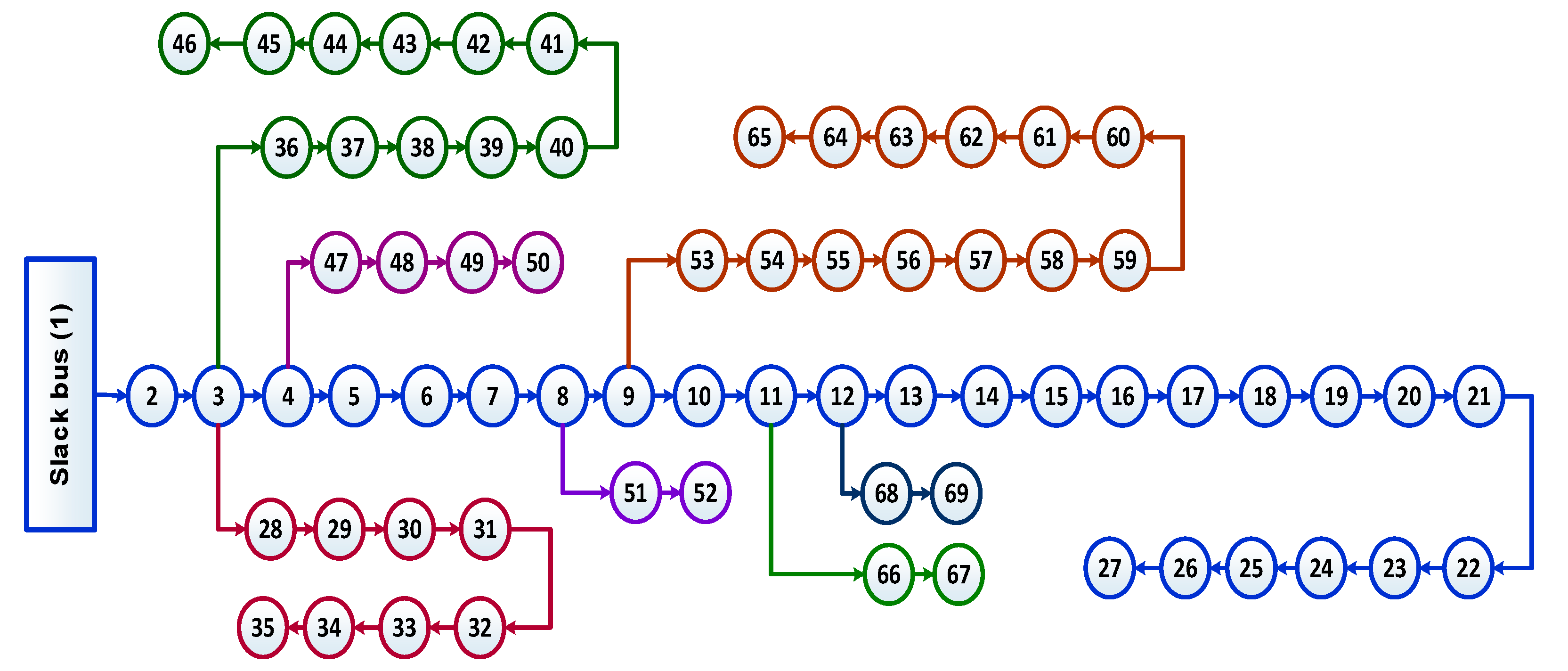
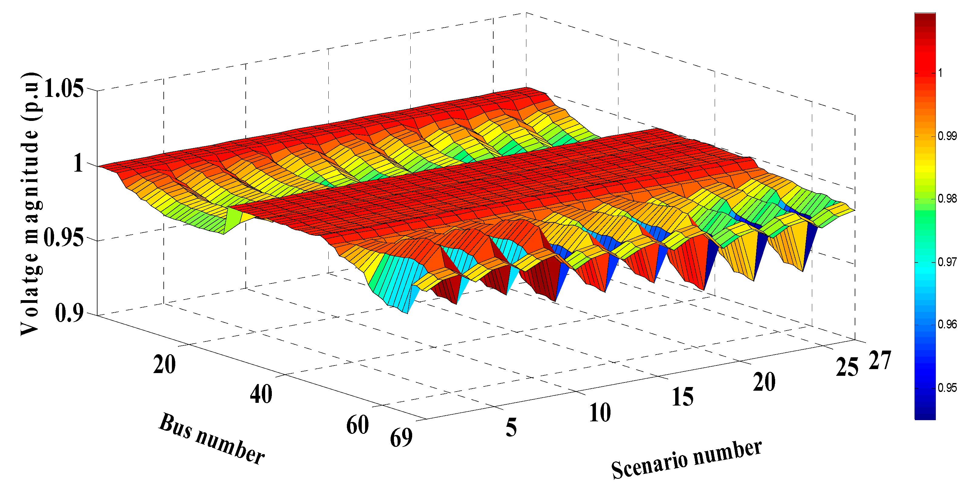
5.1. The IEEE 69-Bus System

The proposed algorithm is utilized to solve the optimal planning of the 69-bus system with optimal integration of RERs considering the uncertainties of the system. Initially, without integration of RERs, the total of the expected values of the power losses ($ET{P}_{Loss}$), the total of the expected values of the voltage deviations ($ETVD$), the total of the expected values of the voltage stability index ($ETVSI$), the expected values of the total cost ($ETCost$), and the expected values of the emissions ($ETEmission$) are 144.0507 kW, 1.4014 p.u, 62.7261 p.u, 2,434,700 USD, and 15.947 × 10³ $\mathrm{kg}/\mathrm{MWh}$, respectively. As mentioned, in Section 3, by combining the load demand, wind speed, and solar irradiance uncertainties, 27 scenarios have been generated to model the uncertainties of the system as depicted in Table 2. By application of the EO, the optimal sites for PV and wind turbine-based DGs are at buses number 26 and 62, respectively, while the optimal rating of the PV and wind turbine-based DGs are 177.5 kW and 1151 kW, respectively.

Table 6. The output powers of renewable energy resources (RERs), the power losses, Voltage Deviations (VD), Voltage Stability Index (VSI), cost, and emission rates for each scenario of IEEE 69-bus system.

Scenario	${\mathit{P}}_{\mathit{w}} \left(kW\right)$	$\mathit{P}{5}_{\mathit{s}} \left(kW\right)$	${\mathit{P}}_{\mathit{L}\mathit{o}\mathit{s}\mathit{s}} \left(MW\right)$	${\mathit{\pi }}_{\mathit{S}}$	$\mathit{V}\mathit{D} \left(pu\right)$	$\mathit{V}\mathit{S}\mathit{I} \left(pu\right)$	$\mathit{C}\mathit{o}\mathit{s}\mathit{t} \left(USD\right)$	$\mathit{E}\mathit{E}\mathit{m}\mathit{i}\mathit{s}\mathit{i}\mathit{o}\mathit{n}$ $\left(kg/MWh\right)$
$\mathrm{S}1$	394.2	74.0592	48.4097	0.0201	0.8028	64.8894	1,071,600	345.9392
$\mathrm{S}2$	939.9	74.0592	12.7234	0.0043	0.3889	66.4681	1,589,600	723.2575
$\mathrm{S}3$	1151	74.0592	12.7201	0.0010	0.318	67.0724	1,785,600	860.2859
$\mathrm{S}4$	394.2	108.4228	47.6489	0.0553	0.7733	65.0009	1,103,800	368.7346
$\mathrm{S}5$	939.9	108.4228	12.2143	0.0119	0.3597	66.581	1,621,700	745.8896
$\mathrm{S}6$	1151	108.4228	12.2965	0.0028	0.2924	67.1859	1,817,700	882.8625
$\mathrm{S}7$	394.2	140.7023	47.0604	0.0499	0.7456	65.1057	1,133,900	390.0656
$\mathrm{S}8$	939.9	140.7023	11.8596	0.0107	0.3323	66.687	1,651,700	767.0688
$\mathrm{S}9$	1151	140.7023	12.0212	0.0026	0.2684	67.2924	1,847,700	903.9902
$\mathrm{S}10$	394.2	74.0592	66.5655	0.0866	1.0111	64.119	1,090,700	353.3142
$\mathrm{S}11$	939.9	74.0592	18.8061	0.0186	0.5899	65.6923	1,612,500	738.4678
$\mathrm{S}12$	1151	74.0592	14.7628	0.0044	0.4346	66.2941	1,809,800	878.1181
$\mathrm{S}13$	394.2	108.4228	65.433	0.2380	0.9813	64.23	1,123,000	376.3508
$\mathrm{S}14$	939.9	108.4228	17.9418	0.0510	0.5603	65.8046	1,644,700	761.3304
$\mathrm{S}15$	1151	108.4228	13.9894	0.0122	0.4051	66.407	1,842,000	900.9217
$\mathrm{S}16$	394.2	140.7023	64.4987	0.2149	0.9534	64.3342	1,153,200	397.9062
$\mathrm{S}17$	939.9	140.7023	17.2566	0.0461	0.5327	65.9101	1,674,900	782.7241
$\mathrm{S}18$	1151	140.7023	13.3886	0.0110	0.3775	66.513	1,872,100	922.2607
$\mathrm{S}19$	394.2	74.0592	91.9413	0.0201	1.2233	63.3491	1,114,300	361.2603
$\mathrm{S}20$	939.9	74.0592	31.2589	0.0043	0.7942	64.9174	1,640,200	754.8008
$\mathrm{S}21$	1151	74.0592	22.9091	0.0010	0.6363	65.5169	1,838,900	897.2459
$\mathrm{S}22$	394.2	108.4228	90.4229	0.0553	1.1932	63.4595	1,146,700	384.5473
$\mathrm{S}23$	939.9	108.4228	30.0269	0.0119	0.7644	65.0292	1,672,500	777.902
$\mathrm{S}24$	1151	108.4228	21.7739	0.0028	0.6065	65.6292	1,871,200	920.2843
$\mathrm{S}25$	394.2	140.7023	89.1295	0.0499	1.165	63.5631	1,177,100	406.3358
$\mathrm{S}26$	939.9	140.7023	28.9996	0.0107	0.7365	65.1342	1,702,800	799.5178
$\mathrm{S}27$	1151	140.7023	20.8364	0.0026	0.5787	65.7347	1,901,400	941.8418

and Figure 4 provide the output power of the PV and wind turbine-based DGs for each scenario, as well as the corresponding $P_{Loss} \left(\mathrm{MW}\right)$, $VD \left(\mathrm{pu}\right)$, $VSI \left(\mathrm{pu}\right)$, $Cost \left(\mathrm{USD}\right)$, and $Emision \left(\mathrm{kg}/\mathrm{MWh}\right).$ As solar irradiance, wind speed, and load demand have different values in each scenario, the yielded result will also be different. At a high probability value which occurred in scenario 13, according to Table 2 the output power of the wind turbine and PV systems is 394.2 kW and 108.4228 kW, respectively.

Table 7. The expected values for each scenario of IEEE 69-bus system.

Scenario	${\mathit{\pi }}_{\mathit{S}}$	$\mathit{E}\mathit{T}{\mathit{P}}_{\mathit{L}\mathit{o}\mathit{s}\mathit{s}} \left(pu\right)$	$\mathit{E}\mathit{T}\mathit{V}\mathit{D} \left(pu\right)$	$\mathit{E}\mathit{T}\mathit{V}\mathit{S}\mathit{I} \left(pu\right)$	$\mathit{E}\mathit{T}\mathit{C}\mathit{o}\mathit{s}\mathit{t} \left(USD\right)$	$\mathit{E}\mathit{T}\mathit{E}\mathit{m}\mathit{i}\mathit{s}\mathit{s}\mathit{i}\mathit{o}\mathit{n}$ $\left(kg/MWh\right)$
$\mathrm{S}1$	0.0201	0.973	0.0161	1.3043	21,540	6.9534
$\mathrm{S}2$	0.0043	0.0547	0.0017	0.2858	6840	3.1100
$\mathrm{S}3$	0.0010	0.0127	0.0003	0.0671	1790	0.8603
$\mathrm{S}4$	0.0553	2.635	0.0428	3.5946	61,040	20.3910
$\mathrm{S}5$	0.0119	0.1453	0.0043	0.7923	19,300	8.8761
$\mathrm{S}6$	0.0028	0.0344	0.0008	0.1881	5090	2.4720
$\mathrm{S}7$	0.0499	2.3483	0.0372	3.2488	56,580	19.4643
$\mathrm{S}8$	0.0107	0.1269	0.0036	0.7136	17,670	8.2076
$\mathrm{S}9$	0.0026	0.0313	0.0007	0.175	4800	2.3504
$\mathrm{S}10$	0.0866	5.7646	0.0876	5.5527	94,460	30.5970
$\mathrm{S}11$	0.0186	0.3498	0.011	1.2219	29,990	13.7355
$\mathrm{S}12$	0.0044	0.065	0.0019	0.2917	7960	3.8637
$\mathrm{S}13$	0.2380	15.573	0.2335	15.2867	267,270	89.5715
$\mathrm{S}14$	0.0510	0.915	0.0286	3.356	83,880	38.8278
$\mathrm{S}15$	0.0122	0.1707	0.0049	0.8102	22,470	10.9912
$\mathrm{S}16$	0.2149	13.8608	0.2049	13.8254	247,830	85.5101
$\mathrm{S}17$	0.0461	0.7955	0.0246	3.0385	77,210	36.0836
$\mathrm{S}18$	0.0110	0.1473	0.0042	0.7316	20,590	10.1449
$\mathrm{S}19$	0.0201	1.848	0.0246	1.2733	22,400	7.2613
$\mathrm{S}20$	0.0043	0.1344	0.0034	0.2791	7050	3.2456
$\mathrm{S}21$	0.0010	0.0229	0.0006	0.0655	1840	0.8972
$\mathrm{S}22$	0.0553	5.0004	0.066	3.5093	63,410	21.2655
$\mathrm{S}23$	0.0119	0.3573	0.0091	0.7738	19,900	9.2570
$\mathrm{S}24$	0.0028	0.061	0.0017	0.1838	5240	2.5768
$\mathrm{S}25$	0.0499	4.4476	0.0581	3.1718	58,740	20.2762
$\mathrm{S}26$	0.0107	0.3103	0.0079	0.6969	18,220	8.5548
$\mathrm{S}27$	0.0026	0.0542	0.0015	0.1709	4940	2.4488
Summation	1	56.2394	0.8816	64.6087	1,248,050	467.7936

provides the expected values for each scenario with optimal integration of RERs. According to Table 7, the summation of the expected values including $ET{P}_{Loss}$, $ETVD$, $ETVSI$, $ETCost$ and $ETEmission$ are enhanced to be 56.2394 kW, 0.8816 p.u, 64.6087 p.u, 1,248,050 USD, and 4,677.936 × 10³ $\mathrm{kg}/\mathrm{MWh}$, respectively.

In other words, the enhancement in the summation of the expected values with optimal integration of the RERs including ${\mathit{ETP}}_{\mathit{Loss}}$, $\mathit{ETVD}$, $\mathit{ETVSI}$, $\mathit{ETCost}$, and $\mathit{ETEmission}$ are 60.95%, 37.09%, 2.91%, 48.73%, and 70.66%, respectively. Figure 5 shows the voltage profile for the obtained scenarios. From this figure, it is obvious that the voltage magnitudes of all scenarios are within the allowable limits, and there is no violation which occurred.

Table 8. A comparison of the obtained results by the application of the investigated algorithms for the IEEE 69-bus system.

Algorithm	Average	Best Solution	Worst Solution	Standard Deviation
SCA	0.3660	0.3621	0.3851	0.0077
PSO	0.3934	0.3617	0.4505	0.0290
ALO	0.3928	0.3636	0.4147	0.0194
EO	0.3616	0.3609	0.3624	0.0006

shows a comparison of the obtained results by the application of other algorithms for the IEEE 69-bus system. Judging from Table 8, the minimum objective function has been obtained by the application of the EO compared with SCA, ALO, and PSO.

5.2. The IEEE 94-Bus System

The optimal planning of the 94-bus system with the optimal integration of RERs considering the uncertainties of the system has been solved by the proposed algorithm. Initially, without the integration of RERs, the total of the expected values of the power losses (${\mathit{ETP}}_{\mathit{Loss}}$), the total of the expected values of the voltage deviations ($\mathit{ETVD}$), the total of the expected values of the voltage stability index ($\mathit{ETVSI}$), the expected values of the total cost ($\mathit{ETCost}$), and the expected values of the emissions ($\mathit{ETEmission}$) are 204.6913 kW, 7.2162 p.u, 67.8052 p.u, 3,103,600 USD, and 20,254 × 103 $\mathrm{kg}/\mathrm{MWh}$, respectively. As referenced in Section 3, by combining load demand, wind speed, and solar irradiance uncertainties, 27 scenarios have been generated to model the uncertainties of the system as shown in Table 2. By utilization of the EO, the optimal sites for PV and wind turbine-based DGs are at buses number 91 and 23, respectively, while the optimal rating of the PV and wind turbine-based DGs are 107.5 kW and 1261.6 kW, respectively.

Table 9. The output powers of RERs, the power losses, Voltage Deviations (VD), Voltage Stability Index (VSI), cost, and emission rates for each scenario of the IEEE 94-bus system.

Scenario	${\mathit{P}}_{\mathit{w}} \left(kW\right)$	${\mathit{P}}_{\mathit{s}} \left(kW\right)$	${\mathit{P}}_{\mathit{L}\mathit{o}\mathit{s}\mathit{s}} \left(MW\right)$	${\mathit{\pi }}_{\mathit{S}}$	$\mathit{V}\mathit{D} \left(pu\right)$	$\mathit{V}\mathit{S}\mathit{I} \left(pu\right)$	$\mathit{C}\mathit{o}\mathit{s}\mathit{t} \left(USD\right)$	$\mathit{E}\mathit{E}\mathit{m}\mathit{i}\mathit{s}\mathit{s}\mathit{i}\mathit{o}\mathit{n}$ $\left(kg/MWh\right)$
$\mathrm{S}1$	432.2	44.5187	74.0228	0.0201	4.1453	77.6061	1,144,200	355.6937
$\mathrm{S}2$	1030.5	44.5187	52.827	0.0043	1.5785	86.8996	1,706,500	757.7621
$\mathrm{S}3$	1262	44.5187	62.2786	0.0010	1.2001	90.5301	1,918,400	901.8688
$\mathrm{S}4$	432.2	65.1755	72.9507	0.0553	4.0964	77.7732	1,163,700	369.7955
$\mathrm{S}5$	1030.5	65.1755	52.801	0.0119	1.5339	87.0723	1,725,600	771.1849
$\mathrm{S}6$	1262	65.1755	62.5802	0.0028	1.207	90.705	1,937,500	915.0791
$\mathrm{S}7$	432.2	84.5794	72.0738	0.0499	4.0507	77.9294	1,182,000	382.9575
$\mathrm{S}8$	1030.5	84.5794	52.8868	0.0107	1.5015	87.2339	1,743,600	783.7222
$\mathrm{S}9$	1262	84.5794	62.9677	0.0026	1.2138	90.8688	1,955,400	927.4206
$\mathrm{S}10$	432.2	44.5187	112.9715	0.0866	4.987	74.7688	1,179,600	367.2078
$\mathrm{S}11$	1030.5	44.5187	75.2483	0.0186	2.3577	83.974	1,747,100	780.0024
$\mathrm{S}12$	1262	44.5187	79.4775	0.0044	1.453	87.5682	1,960,700	927.4984
$\mathrm{S}13$	432.2	65.1755	111.2094	0.2380	4.9359	74.9366	1,199,300	381.7574
$\mathrm{S}14$	1030.5	65.1755	74.644	0.0510	2.3114	84.1472	1,766,400	793.8006
$\mathrm{S}15$	1262	65.1755	79.2327	0.0122	1.4557	87.7437	1,979,900	941.0633
$\mathrm{S}16$	432.2	84.5794	109.6941	0.2149	4.8884	75.0935	1,217,800	395.3338
$\mathrm{S}17$	1030.5	84.5794	74.1937	0.0461	2.2683	84.3093	1,784,600	806.6858
$\mathrm{S}18$	1262	84.5794	79.1134	0.0110	1.4596	87.9079	1,998,000	953.7337
$\mathrm{S}19$	432.2	44.5187	166.2304	0.0201	5.8647	71.9096	1,224,200	380.0133
$\mathrm{S}20$	1030.5	44.5187	110.2486	0.0043	3.1668	81.0279	1,797,400	804.6575
$\mathrm{S}21$	1262	44.5187	108.7544	0.0010	2.1969	84.586	2,012,800	955.8679
$\mathrm{S}22$	432.2	65.1755	163.7147	0.0553	5.8113	72.0782	1,244,100	395.052
$\mathrm{S}23$	1030.5	65.1755	109.0211	0.0119	3.1187	81.2017	1,817,000	818.8602
$\mathrm{S}24$	1262	65.1755	107.9232	0.0028	2.1504	84.762	2,032,300	969.8134
$\mathrm{S}25$	432.2	84.5794	161.5027	0.0499	5.7616	72.2358	1,262,900	409.0805
$\mathrm{S}26$	1030.5	84.5794	107.9934	0.0107	3.0738	81.3643	1,835,300	832.1201
$\mathrm{S}27$	1262	84.5794	107.2602	0.0026	2.107	84.9267	2,050,500	982.8367

and Figure 6 provide the output power of the PV and wind turbine-based DGs for each scenario, as well as the corresponding $P_{Loss} \left(\mathrm{MW}\right)$, $VD \left(\mathrm{pu}\right)$, $VSI \left(\mathrm{pu}\right)$, $Cost \left(\mathrm{USD}\right)$, and $Emision \left(\mathrm{kg}/\mathrm{MWh}\right).$ As solar irradiance, wind speed, and load demand have different values in each scenario, the yielded result will also be different. At a high probability value which occurred in scenario 13 according to Table 2, the output power of the wind turbine and PV systems are 432.2 kW and 65.1755 kW, respectively.

Table 10. The expected values for each scenario of the 94-bus system.

Scenario	${\mathit{\pi }}_{\mathit{S}}$	$\mathit{E}\mathit{T}{\mathit{P}}_{\mathit{L}\mathit{o}\mathit{s}\mathit{s}} \left(kW\right)$	$\mathit{E}\mathit{T}\mathit{V}\mathit{D} \left(pu\right)$	$\mathit{E}\mathit{T}\mathit{V}\mathit{S}\mathit{I} \left(pu\right)$	$\mathit{E}\mathit{T}\mathit{C}\mathit{o}\mathit{s}\mathit{t} \left(USD\right)$	$\mathit{E}\mathit{T}\mathit{E}\mathit{m}\mathit{i}\mathit{s}\mathit{s}\mathit{i}\mathit{o}\mathit{n}$ $\left(kg/MWh\right)$
$\mathrm{S}1$	0.0201	1.4879	0.0833	1.5599	23,000	71,494
$\mathrm{S}2$	0.0043	0.2272	0.0068	0.3737	7340	32,584
$\mathrm{S}3$	0.0010	0.0623	0.0012	0.0905	1920	9019
$\mathrm{S}4$	0.0553	4.0342	0.2265	4.3009	64,350	204,497
$\mathrm{S}5$	0.0119	0.6283	0.0183	1.0362	20,540	91,771
$\mathrm{S}6$	0.0028	0.1752	0.0034	0.254	5430	25,622
$\mathrm{S}7$	0.0499	3.5965	0.2021	3.8887	58,980	191,096
$\mathrm{S}8$	0.0107	0.5659	0.0161	0.9334	18,660	83,858
$\mathrm{S}9$	0.0026	0.1637	0.0032	0.2363	5080	24,113
$\mathrm{S}10$	0.0866	9.7833	0.4319	6.475	102,150	318,002
$\mathrm{S}11$	0.0186	1.3996	0.0439	1.5619	3,2500	145,080
$\mathrm{S}12$	0.0044	0.3497	0.0064	0.3853	8630	40,810
$\mathrm{S}13$	0.2380	26.4678	1.1748	17.8349	285,440	908,583
$\mathrm{S}14$	0.0510	3.8068	0.1179	4.2915	90,090	404,838
$\mathrm{S}15$	0.0122	0.9666	0.0178	1.0705	24,160	114,810
$\mathrm{S}16$	0.2149	23.5733	1.0505	16.1376	261,710	849,572
$\mathrm{S}17$	0.0461	3.4203	0.1046	3.8867	82,270	371,882
$\mathrm{S}18$	0.0110	0.8702	0.0161	0.967	21,980	104,911
$\mathrm{S}19$	0.0201	3.3412	0.1179	1.4454	24,610	76,383
$\mathrm{S}20$	0.0043	0.4741	0.0136	0.3484	7730	34,600
$\mathrm{S}21$	0.0010	0.1088	0.0022	0.0846	2010	9559
$\mathrm{S}22$	0.0553	9.0534	0.3214	3.9859	68,800	218,464
$\mathrm{S}23$	0.0119	1.2974	0.0371	0.9663	21,620	97,444
$\mathrm{S}24$	0.0028	0.3022	0.006	0.2373	5690	27,155
$\mathrm{S}25$	0.0499	8.059	0.2875	3.6046	63,020	204,131
$\mathrm{S}26$	0.0107	1.1555	0.0329	0.8706	19,640	89,037
$\mathrm{S}27$	0.0026	0.2789	0.0055	0.2208	5330	25,554
Summation	1	105.6493	4.3489	77.0479	1,332,680	4,774,869

provides the expected values for each scenario with the optimal integration of RERs. According to Table 10, the summation of the expected values including $ET{P}_{Loss}$, $ETVD$, $ETVSI$, $ETCost$, and $ETEmission$ are enhanced to be 105.6493 kW, 4.3489 p.u, 77.0479 p.u, 1,332,680 USD, and 4774.689 × 10³ $\mathrm{kg}/\mathrm{MWh}$, respectively. In other words, the enhancement in the summation of the expected values with optimal integration of the RERs including $E{P}_{Loss}$, $EVD$, $ETVSI$, $ETCost$, and $\mathit{EEmission}$ are 48.38, 39.73%, 11.99%, 57.06%, and 76.42%, respectively. Figure 7 shows the voltage profile for the obtained scenarios.

From this figure, it is obvious that the voltage magnitudes of all scenarios are within the allowable limits, and no violation occurred.

Table 11. A comparison of the obtained results by the application of the investigated algorithms on the 94-bus system.

Algorithm	Average	Best Solution	Worst Solution	SD
SCA	0.3546	0.3543	0.3562	0.0005
PSO	0.3738	0.3621	0.4141	0.0160
ALO	0.3898	0.3544	0.4879	0.0424
EO	0.3543	0.3535	0.3564	0.0008

shows a comparison of the obtained results by the application of other algorithms for the 94-bus system. Judging from Table 11, the minimum objective function has been obtained by the application of the EO compared with SCA, ALO, and PSO.

6. Conclusions

In this paper, the optimal planning for distribution systems has been solved using an efficient stochastic framework by assigning the optimal sites and sizes of solar PV and wind turbine-based DGs under uncertainties of load demands, wind speeds, and solar radiation. The proposed framework is based on application of the Equilibrium Optimizer (EO) and the scenario-based method for reducing the expected power loss, the expected system voltage deviations, the expected total cost, the expected total emissions, and maximizing the expected voltage stability. The EO has been applied for solving the allocation problem of solar PV and wind turbine-based DGs, while the scenario-based method was utilized to represent the combination the uncertainties of load demands, wind speeds, and solar radiation. The proposed technique has been implemented on an IEEE 69-bus and 94-bus practical distribution system located in Portugal, and the obtained results were compared with those obtained by SCA, PSO, and ALO. The obtain results verified the following:

-

The effectiveness of the proposed framework for solving the optimal planning problem for distribution systems.

-

The superiority of the EO for assigning the optimal placement and sizes of the DGs compared to SCA, PSO, and ALO techniques.

-

The inclusion of solar PV and wind turbine-based DGs using the proposed method in the IEEE 69-bus system can reduce the expected power losses, voltage deviations, cost, and emissions rate and enhance the voltage stability compared to the base case by 60.95%, 37.09%, 2.91%, 70.66%, and 48.73%, respectively.

-

The inclusion of solar PV and wind turbine-based DGs using the proposed method in a 94-bus system can reduce the expected power losses, voltage deviations, cost, and emissions rate and enhance the voltage stability compared to the base case by 48.38%, 39.73%, 57.06%, 76.42%, and 11.99%, respectively.

References

1. Ganguly, S.; Sahoo, N.; Das, D. Recent advances on power distribution system planning: A state-of-the-art survey. Energy Syst. 2013, 4, 165–193. [Google Scholar] [CrossRef]
2. Sims, R.E.; Rogner, H.-H.; Gregory, K. Carbon emission and mitigation cost comparisons between fossil fuel, nuclear and renewable energy resources for electricity generation. Energy Policy 2003, 31, 1315–1326. [Google Scholar] [CrossRef]
3. Ehsan, A.; Yang, Q. Active distribution system reinforcement planning with EV charging stations—Part I: Uncertainty modeling and problem formulation. IEEE Trans. Sustain. Energy 2019, 11, 970–978. [Google Scholar] [CrossRef]
4. Cervantes, J.; Choobineh, F. Optimal sizing of a nonutility-scale solar power system and its battery storage. Appl. Energy 2018, 216, 105–115. [Google Scholar] [CrossRef]
5. Lai, C.S.; Jia, Y.; Lai, L.L.; Xu, Z.; McCulloch, M.D.; Wong, K.P. A comprehensive review on large-scale photovoltaic system with applications of electrical energy storage. Renew. Sustain. Energy Rev. 2017, 78, 439–451. [Google Scholar] [CrossRef]
6. Xavier, G.A.; Martins, J.H.; Monteiro, P.M.d.B.; Diniz, A.S.A.C.; Diniz, A.C. Simulation of distributed generation with photovoltaic microgrids—Case study in Brazil. Energies 2015, 8, 4003–4023. [Google Scholar] [CrossRef]
7. Weckx, S.; D’hulst, R.; Driesen, J. Locational pricing to mitigate voltage problems caused by high PV penetration. Energies 2015, 8, 4607–4628. [Google Scholar] [CrossRef] [Green Version]
8. Georgilakis, P.S.; Hatziargyriou, N.D. A review of power distribution planning in the modern power systems era: Models, methods and future research. Electr. Power Syst. Res. 2015, 121, 89–100. [Google Scholar] [CrossRef]
9. Gao, Y.; Liu, J.; Yang, J.; Liang, H.; Zhang, J. Multi-objective planning of multi-type distributed generation considering timing characteristics and environmental benefits. Energies 2014, 7, 6242–6257. [Google Scholar] [CrossRef]
10. El-Khattam, W.; Hegazy, Y.; Salama, M. An integrated distributed generation optimization model for distribution system planning. IEEE Trans. Power Syst. 2005, 20, 1158–1165. [Google Scholar] [CrossRef]
11. Liu, Z.; Wen, F.; Ledwich, G. Optimal siting and sizing of distributed generators in distribution systems considering uncertainties. IEEE Trans. Power Deliv. 2011, 26, 2541–2551. [Google Scholar] [CrossRef]
12. Shaaban, M.F.; El-Saadany, E. Accommodating high penetrations of PEVs and renewable DG considering uncertainties in distribution systems. IEEE Trans. Power Syst. 2013, 29, 259–270. [Google Scholar] [CrossRef]
13. Zeng, B.; Zhang, J.; Zhang, Y.; Yang, X.; Dong, J.; Liu, W. Active distribution system planning for low-carbon objective using cuckoo search algorithm. J. Electr. Eng. Technol. 2014, 9, 433–440. [Google Scholar] [CrossRef] [Green Version]
14. Peng, X.; Lin, L.; Zheng, W.; Liu, Y. Crisscross optimization algorithm and Monte Carlo simulation for solving optimal distributed generation allocation problem. Energies 2015, 8, 13641–13659. [Google Scholar] [CrossRef] [Green Version]
15. Esmaeili, M.; Sedighizadeh, M.; Esmaili, M. Multi-objective optimal reconfiguration and DG (Distributed Generation) power allocation in distribution networks using Big Bang-Big Crunch algorithm considering load uncertainty. Energy 2016, 103, 86–99. [Google Scholar] [CrossRef]
16. Santos, S.F.; Fitiwi, D.Z.; Bizuayehu, A.W.; Shafie-Khah, M.; Asensio, M.; Contreras, J.; Cabrita, C.M.P.; Catalao, J.P. Novel multi-stage stochastic DG investment planning with recourse. IEEE Trans. Sustain. Energy 2016, 8, 164–178. [Google Scholar] [CrossRef]
17. Kroposki, B.; Sen, P.K.; Malmedal, K. Optimum sizing and placement of distributed and renewable energy sources in electric power distribution systems. IEEE Trans. Ind. Appl. 2013, 49, 2741–2752. [Google Scholar] [CrossRef]
18. Baghaee, H.; Mirsalim, M.; Gharehpetian, G.; Talebi, H. Reliability/cost-based multi-objective Pareto optimal design of stand-alone wind/PV/FC generation microgrid system. Energy 2016, 115, 1022–1041. [Google Scholar] [CrossRef]
19. Saric, M.; Hivziefendic, J.; Konjic, T.; Ktena, A. Distributed generation allocation considering uncertainties. Int. Trans. Electr. Energy Syst. 2018, 28, e2585. [Google Scholar] [CrossRef]
20. Zhao, B.; Guo, C.; Cao, Y. A multiagent-based particle swarm optimization approach for optimal reactive power dispatch. IEEE Trans. Power Syst. 2005, 20, 1070–1078. [Google Scholar] [CrossRef]
21. Abdel-Fatah, S.; Ebeed, M.; Kamel, S. Optimal Reactive Power Dispatch Using Modified Sine Cosine Algorithm. In Proceedings of the 2019 International Conference on Innovative Trends in Computer Engineering (ITCE), Aswan, Egypt, 2–4 February 2019; pp. 510–514. [Google Scholar]
22. Sulaiman, M.; Rashid, M.M.; Aliman, O.; Mohamed, M.; Ahmad, A.; Bakar, M. Loss minimisation by optimal reactive power dispatch using cuckoo search algorithm. In Proceedings of the 3rd IET International Conference on Clean Energy and Technology (CEAT) 2014, Kuching, Malaysia, 24–26 November 2014. [Google Scholar]
23. Heidari, A.A.; Abbaspour, R.A.; Jordehi, A.R. Gaussian bare-bones water cycle algorithm for optimal reactive power dispatch in electrical power systems. Appl. Soft Comput. 2017, 57, 657–671. [Google Scholar] [CrossRef]
24. Li, Z.; Cao, Y.; Dai, L.V.; Yang, X.; Nguyen, T.T. Finding solutions for optimal reactive power dispatch problem by a novel improved antlion optimization algorithm. Energies 2019, 12, 2968. [Google Scholar] [CrossRef] [Green Version]
25. Villa-Acevedo, W.M.; López-Lezama, J.M.; Valencia-Velásquez, J.A. A novel constraint handling approach for the optimal reactive power dispatch problem. Energies 2018, 11, 2352. [Google Scholar] [CrossRef] [Green Version]
26. Abou El-Ela, A.; Kinawy, A.; El-Sehiemy, R.; Mouwafi, M. Optimal reactive power dispatch using ant colony optimization algorithm. Electr. Eng. 2011, 93, 103–116. [Google Scholar] [CrossRef]
27. Sakr, W.S.; El-Sehiemy, R.A.; Azmy, A.M. Adaptive differential evolution algorithm for efficient reactive power management. Appl. Soft Comput. 2017, 53, 336–351. [Google Scholar] [CrossRef]
28. Khazali, A.; Kalantar, M. Optimal reactive power dispatch based on harmony search algorithm. Int. J. Electr. Power Energy Syst. 2011, 33, 684–692. [Google Scholar] [CrossRef]
29. Dai, C.; Chen, W.; Zhu, Y.; Zhang, X. Seeker optimization algorithm for optimal reactive power dispatch. IEEE Trans. Power Syst. 2009, 24, 1218–1231. [Google Scholar]
30. Mandal, B.; Roy, P.K. Optimal reactive power dispatch using quasi-oppositional teaching learning based optimization. Int. J. Electr. Power Energy Syst. 2013, 53, 123–134. [Google Scholar] [CrossRef]
31. Faramarzi, A.; Heidarinejad, M.; Stephens, B.; Mirjalili, S. Equilibrium optimizer: A novel optimization algorithm. Knowl.-Based Syst. 2020, 191, 105190. [Google Scholar] [CrossRef]
32. Ramadan, A.; Ebeed, M.; Kamel, S.; Nasrat, L. Optimal power flow for distribution systems with uncertainty. In Uncertainties in Modern Power Systems; Elsvier: Amsterdam, The Netherlands, 2020; pp. 145–162. [Google Scholar]
33. Bastawy, M.; Ebeed, M.; Rashad, A.; Alghamdi, A.S.; Kamel, S. Micro-Grid Dynamic Economic Dispatch with Renewable Energy Resources Using Equilibrium Optimizer. In Proceedings of the 2020 IEEE Electric Power and Energy Conference (EPEC), Edmonton, AB, Canada, 9–10 November 2020; pp. 1–5. [Google Scholar]
34. Özkaya, H.; Yıldız, M.; Yıldız, A.R.; Bureerat, S.; Yıldız, B.S.; Sait, S.M. The equilibrium optimization algorithm and the response surface-based metamodel for optimal structural design of vehicle components. Mater. Test. 2020, 62, 492–496. [Google Scholar] [CrossRef]
35. Abdel-Basset, M.; Mohamed, R.; Mirjalili, S.; Chakrabortty, R.K.; Ryan, M.J. Solar photovoltaic parameter estimation using an improved equilibrium optimizer. Sol. Energy 2020, 209, 694–708. [Google Scholar] [CrossRef]
36. Gampa, S.R.; Das, D. Optimum placement and sizing of DGs considering average hourly variations of load. Int. J. Electr. Power Energy Syst. 2015, 66, 25–40. [Google Scholar] [CrossRef]
37. Soroudi, A.; Aien, M.; Ehsan, M. A probabilistic modeling of photo voltaic modules and wind power generation impact on distribution networks. IEEE Syst. J. 2011, 6, 254–259. [Google Scholar] [CrossRef] [Green Version]
38. Mohseni-Bonab, S.M.; Rabiee, A. Optimal reactive power dispatch: A review, and a new stochastic voltage stability constrained multi-objective model at the presence of uncertain wind power generation. IET Gener. Transm. Distrib. 2017, 11, 815–829. [Google Scholar] [CrossRef]
39. Ebeed, M.; Alhejji, A.; Kamel, S.; Jurado, F. Solving the Optimal Reactive Power Dispatch Using Marine Predators Algorithm Considering the Uncertainties in Load and Wind-Solar Generation Systems. Energies 2020, 13, 4316. [Google Scholar] [CrossRef]
40. Hetzer, J.; David, C.Y.; Bhattarai, K. An economic dispatch model incorporating wind power. IEEE Trans. Energy Convers. 2008, 23, 603–611. [Google Scholar] [CrossRef]
41. Biswas, P.P.; Suganthan, P.N.; Mallipeddi, R.; Amaratunga, G.A.J. Optimal reactive power dispatch with uncertainties in load demand and renewable energy sources adopting scenario-based approach. Appl. Soft Comput. 2019, 75, 616–632. [Google Scholar] [CrossRef]
42. Atwa, Y.; El-Saadany, E.; Salama, M.; Seethapathy, R. Optimal renewable resources mix for distribution system energy loss minimization. IEEE Trans. Power Syst. 2009, 25, 360–370. [Google Scholar] [CrossRef]
43. Salameh, Z.M.; Borowy, B.S.; Amin, A.R. Photovoltaic module-site matching based on the capacity factors. IEEE Trans. Energy Convers. 1995, 10, 326–332. [Google Scholar] [CrossRef]
44. Liang, R.-H.; Liao, J.-H. A fuzzy-optimization approach for generation scheduling with wind and solar energy systems. IEEE Trans. Power Syst. 2007, 22, 1665–1674. [Google Scholar] [CrossRef]
45. Reddy, S.S.; Bijwe, P.; Abhyankar, A.R. Real-time economic dispatch considering renewable power generation variability and uncertainty over scheduling period. IEEE Syst. J. 2014, 9, 1440–1451. [Google Scholar] [CrossRef]
46. Mirjalili, S. SCA: A sine cosine algorithm for solving optimization problems. Knowl.-Based Syst. 2016, 96, 120–133. [Google Scholar] [CrossRef]
47. Eberhart, R.; Kennedy, J. A New Optimizer Using Particle Swarm Theory. In Proceedings of the Sixth International Symposium on Micro Machine and Human Science (MHS’95), Nagoya, Japan, 4–6 October 1995; pp. 39–43. [Google Scholar]
48. Mirjalili, S. The ant lion optimizer. Adv. Eng. Softw. 2015, 83, 80–98. [Google Scholar] [CrossRef]
49. Chandramohan, S.; Atturulu, N.; Devi, R.K.; Venkatesh, B. Operating cost minimization of a radial distribution system in a deregulated electricity market through reconfiguration using NSGA method. Int. J. Electr. Power Energy Syst. 2010, 32, 126–132. [Google Scholar] [CrossRef]
50. Pires, D.F.; Antunes, C.H.; Martins, A.G. NSGA-II with local search for a multi-objective reactive power compensation problem. Int. J. Electr. Power Energy Syst. 2012, 43, 313–324. [Google Scholar] [CrossRef]
Figure 1. Application of the Equilibrium Optimizer (EO) for the optimal power planning solution.
Sustainability 13 03566 g001
Figure 2. The IEEE 69-bus line diagram.
Sustainability 13 03566 g002
Figure 3. The IEEE 94-bus line diagram.
Sustainability 13 03566 g003
Figure 4. The outcomes for each scenario of the IEEE 69-bus system: (a) the photovoltaic (PV) power, (b) the wind turbine (WT) power, (c) the voltage deviations, (d) the voltage stability index, (e) the total cost, (f) the total emission rate, (g) the power loss, and (h) the probability.
Sustainability 13 03566 g004
Figure 5. Voltage profile for each scenario of the 69-bus system.
Sustainability 13 03566 g005
Figure 6. The outcomes for each scenario of the 94-bus system: (a) the PV power, (b) the WT power, (c) the voltage deviations, (d) the voltage stability index, (e) the total cost, (f) the total emission rate, (g) the power loss, and (h) the probability.
Sustainability 13 03566 g006
Figure 7. Voltage profile for each scenario of the 94-bus system.
Sustainability 13 03566 g007