Analysis on the Housing Price Relationship Network of Large and Medium-Sized Cities in China Based on Gravity Model

Abstract

The relationship among cities is getting closer, so are housing prices. Based on the sale price of stocking houses in thirty-five large and medium-sized cities in China from 2010 to 2021, this study established the modified gravity model and used the method of social network analysis to explore the spatial linkage of urban housing prices. The results show that: (1) from the overall network structure, the integration degree of housing price network in China is still at a low stage, and the influence of housing price is polarized; (2) from the individual network structure, Beijing, Shanghai, Shenzhen, Nanjing, Hangzhou, and Hefei have a higher degree of centrality. Chengdu, Xining, Kunming, Urumqi, and Lanzhou stay in an isolation position every year; (3) from the results of cohesive subgroup analysis, different cities play different roles in the block each year and have different influences on other cities. (4) Emergencies, such as outbreaks of COVID-19, also have an impact on the housing price network. Structural divergence among urban housing prices has become more pronounced, and the diversity of house price network has been somewhat reduced. Based on the above findings, this paper puts forward some recommendations for the healthy development of housing market from the perspective of housing price network.

1. Introduction

Housing prices are largely determined by local governments. However, with the increasing connection between regional economies, especially the development and integration of Beijing-Tianjin-Hebei urban agglomeration, Guangdong-Hong Kong-Macao urban agglomeration, and the Yangtze River Delta urban agglomeration—links of housing prices among different cities became more frequent and diverse than before in China [1]. This kind of relationship makes housing prices in different cities have interdependence and mutual influence [2,3], which is not only related to geographical distance but also related to their level of housing prices. According to the housing sales price index of seventy large and medium-sized cities in China in October 2020, although the four metropolises, Beijing, Shanghai, Guangzhou and Shenzhen, are far away from each other, their sales price indices all showed upward trend compared with the previous month. However, in the cities around Beijing such as Tianjin and Shijiazhuang, the sales prices declined. Other provincial capitals like Chengdu, Changsha, Wuhan, and Kunming rose by 0.1–0.5%, but in Zhengzhou, Chongqing, Guiyang decreased by 0.2–0.3%. It can be seen that the housing prices among large and medium-sized cities with a central position in each region are no longer only affected by the housing prices in cities within this region, but also have an attraction or linkage relationship with the cities outside this region, and may form a related urban network [4,5]. With the impact of the COVID-19 outbreak in 2020 on the global economy and housing market, urban housing prices have shown different responses to the impact of such a public health event, including in China.

The housing price relationship among cities can also be called a complex network. There are many methods to study complex networks, including system dynamics [6], community discovery [7], social network analysis (SNA) [8,9,10,11], and so on. In order to explore the relationship among housing prices in different cities and keep the healthy development trend of China’s housing market, this paper uses the SNA method to explore the network structure characteristics of housing price relationships, especially in large and medium-sized cities. The housing price relationship is measured by the modified gravity model, which integrates the geographical location and the level of housing prices. The following issue is also analyzed and discussed. How will the network relationship of housing prices between cities evolve? What role do different cities play in the structural change? How does the urban housing price network respond to emergencies? How can we control the irrational rise of housing prices caused by the complex relationship among cities?

The rest of the paper is organized as follows: Section 2 gives a brief review of previous relevant studies. Section 3 introduces the research methods and data sources. Section 4 presents the result of empirical analysis. Section 5 is the discussion, and Section 6 puts forward the research conclusions and corresponding policy recommendations.

2. Literature Review

2.1. Spatial Relationship of the Housing Price

With the development of urban elements, urban housing prices no longer exist independently, and the interaction between multiple cities is more and more complex. Many foreign studies have proved that the multi-dimensional intercity correlation made the urban housing market more closely linked. As early as 1995, Drake compared with different parts of the housing price in the UK, there were clear regional differences in the housing price movements [12]. Meen pointed out that the housing market in the UK was characterized by a series of interrelated local markets rather than a single national market [13]. Based on the regional relevance of housing prices, Clapp and Tirtiroglu, have confirmed that there was a spillover effect between housing prices [14]. Holly et al. put forward the view that the spillover effect of neighboring cities was more intense, that is, the price changes of a city spread to neighboring cities at the beginning, and then spread to other areas [15]. However, this spillover phenomenon does not only exist between neighboring cities. Many scholars have proved that the cross-regional linkage of the housing market strengthened the interdependence of the entire market [16,17,18,19,20].

In the Chinese real estate market, the inter-regional interaction of housing prices was very significant. On the one hand, the interaction between housing prices in different cities was obvious. From the perspective of the geographical distribution of urban housing prices in China, there were large differences in housing price fluctuations among the different regions, different urban agglomerations, and different cities [21]. The spillover phenomenon of housing price showed that the central city spilled over to the margin, the housing prices of the first-tier, second-tier, and third-tier cities showed an excessive echelon trend and the positive impulse of housing price in different “core cities” can lead to the rise or fall in other housing prices [22,23,24,25]. On the other hand, some scholars believed that a few cities had no interactive relationship between housing prices. For example, in Taiwan as the core city, Taipei had not spread to the surrounding areas and was isolated [26]. Zhang and Lin pointed out that as the core city Guangzhou dominated the fluctuation of housing prices in China, but Beijing, Shenyang, and Chongqing showed independence [27].

It can be seen that the correlation between urban housing prices is a reality that cannot be ignored. However, with different methods, research periods and sample cities were used, scholars draw different conclusions on the interaction mechanism of housing price and the strength of the relationship.

2.2. The Gravity Model

Due to the acceleration of economic globalization and marketization, various resources and elements between cities have a strong mutual attraction. As a measure of the relationship, the gravity model originated from the formula of universal gravitation in physics, which considering the quality and geographical factors, can fully show the spatial effect of city elements attracting. The gravity model is used to measure the spatial relationship and has been widely used in urban transportation [28], commodity and energy [29,30], sustainable development [31,32], and other fields in the urban network.

Based on the modified gravity model, Chinese scholar Zeng et al. measured the suitability degree of twenty-one public rental housing in nine districts of Chongqing from the perspective of location selection [33]. Mao and Wang analyzed the influence factors and mechanisms of population flow based on the gravity model according to the provincial population flow data of China’s census, which focused on the impact of affordable housing on interprovincial population mobility [34]. Cheng and Zhang derived a theoretical model to measure the ripple effect of housing prices in China based on the gravity model under the coordinated development strategy of Beijing–Tianjin–Hebei urban agglomeration [35]. Li. extended the classical gravity model to measure the spatial scope of the Shenzhen metropolitan area, effectively defined the “radius” of housing and transportation infrastructure policy, and provided a basis for planning the scale of the metropolitan area reasonably [36].

Previous studies have modified the gravity model and applied it to different research fields, including the spillover effects and influencing factors in the housing market, but did not consider the interaction between housing prices in different cities. Based on the previous research results, this paper constructs a modified gravity model to measure the interaction of urban housing prices of cities by considering the housing price in each city and distance between cities. This kind of relationship can be extended by the method of SNA.

2.3. Social Network Analysis

The concept of the social network was first proposed by British anthropologist Radcliffe in 1940. Later, anthropologist Barnes (1954) of the University of Manchester in the UK put forward a more mature social network analysis when studying the hierarchical structure of a diocese on a small island in Western Norway [37]. Becker (1974) combined the concept of social network with modern consumer demand theory for the first time and applied it to the field of economics [38]. Barry Wellman (1999) proposed that “social network analysis had scientific quantitative methods and models in the process of describing relationship structure and analyzed the influence of relationship on individual behavior, which played an important role”. So far, this method has been widely used in the field of sociology [39], psychology [40], medicine [41], economics [42], and management [43].

In recent years, Chinese scholars have applied SNA to the spatial network structure of urban housing prices. In the existing research, Chen et al. constructed the model of VAR and used the method of SNA to study the structural characteristics and the influence factors of linkage networks among house prices in sixty-nine large and medium-sized cities in China. It was found that different cities belong to different sectors, which played different roles in the housing network [4]. Fang and Pei used the SNA to analysis the sales prices of commercial housing in thirty-five major cities in China. It was found that the density and correlation degree of the urban housing price was with an upward trend, the network hierarchy was at a high level, and the efficiency was gradually stable [44]. Wang et al. also analyzed the spatial linkage effect of housing prices in the Beijing–Tianjin–Hebei urban agglomeration through the SNA and found that Beijing, Tianjin, Shijiazhuang played a leading role in the housing linkage network [45].

Previous studies have considered the causal relationship between housing prices in different cities or the influence of society and economy on housing price, but have not considered the influence of housing price gap in different cities and the status of urban housing price in the whole network on the housing price relationship. This paper aims to explore the dynamic changes of the spatial relationship between housing prices in thirty-five large and medium-sized cities in China. Therefore, we consider the factors such as geographical distance, the radiation range and attractiveness of housing prices, the directionality of the housing price relationship, and the isolated node problem caused by the strength of attraction at the same time.

3. Research Methods and Source of Data

3.1. Social Network Analysis Method

SNA is an analysis method to discuss the network structure and attribute characteristics by taking the relationship in the network as the basic unit. Urban housing price network has the same characteristics as a social network, such as:

Due to the diversity of network nodes, the housing price nodes in each city are different.

Owing to the complexity of network structure, the relationship between urban housing prices is complicated.

The network is dynamic changes, that is, different cities have different positions and roles in the network at different times [46].

Therefore, the network relationship of urban housing prices can be studied by the method of SNA.

3.2. Construction of Housing Price Relationship Network in Large and Medium-Sized Cities Based on Gravity Model

The method of SNA takes the node as the object and the relationship between two nodes as the basic analysis unit [30]. Therefore, the determination of “relationship” is significantly important in the construction of the urban housing price network. The urban housing price network refers to a network of relationships with turban housing price as the node and the transmission of fluctuation in urban housing price as the link. As the relationship between urban housing prices was very complex, this research used the gravity model for reference and put forward the following hypotheses. On the one hand, due to the gap between housing prices in different cities, cities with low housing prices would be attracted by the cities with high housing prices, while the attraction relationship of housing price will weaken as the increase of distance. On the other hand, the level of different housing prices in the overall housing price network was different, and the radiation of price to other regions is also different.

In this study, the gap of housing prices represents the attractiveness of housing prices and is used as the gravity coefficient in the gravity model. The proportion of housing price in the sample cities represents the housing price level, which is like the quality of gravity model. The gravity model also is modified with geographical distance to determine the spatial attractiveness between urban housing prices. The modified gravity model and descriptive of the variables were as follows:

$$F_{ij}=G_{ij}\frac{M_i{m}_j}{R_{ij}{}^2}=G_{ij}\times M_i\times m_j\times R_{ij}{}^{-2}$$

(1)

$$G_{ij}=\frac{P_i-P_j}{P_{max}-P_{min}}$$

(2)

$$M_i=\frac{P_i}{P_{max}}$$

(3)

$$m_j=\frac{P_j}{P_{max}}$$

(4)

$$R_{ij}{}^{-2}=\frac{r_{ij}{}^{-2}}{r_{max}{}^{-2}}$$

(5)

From the

Table 1. The descriptive of the variable.

Variable Name	Meaning of Variables	Range
Fij	Fij represents the attractiveness of the housing prices of city i to the housing prices of city j.	$-1\le F_{ij}\le$1
Gij	Gij is the gravity coefficient of housing price of city i to the housing price of city j in the whole urban housing price network.	$-1\le G_{ij}\le$1
Mi	Mi is the housing price level of city i.	$0<M_i\le$1
mj	mj is the housing price level of city j.	$0<m_j\le$1
Pi	Pi is the housing price of city i.	-
Pj	Pj is the housing price of city j.	-
Pmax	Pmax is the maximum value of housing price.	-
Pmin	Pmin is the minimum value of housing price.	-
Rij	Rij is the sphere distance coefficient between city i and city j.	$0\le R_{ij}\le$1
rij	rij is the sphere distance between city i and city j.	-
rmax	rmax is the maximum sphere distance between sample cities.	-

, it is important to note that:

F_ij represents the attractiveness of the housing prices of city i to the housing prices of city j.

G_ij can be expressed as the ratio of the gap between housing prices of city i and city j to the maximum difference of the housing prices in the city, and which can be expressed by the ratio of the gap between different housing price of city i and city j to the maximum difference of the housing prices in the sample cities. When the housing price of city i is greater than that in city j, the value is positive, indicating that the housing price of city i is positively attractive to the housing price of city j. When the housing price of city j is greater than that of city i, the value is negative, indicating that the housing price of city i is attracted by the housing price of city j.

M_i and m_j can be expressed by the ratio of housing price of city i (P_i) to the highest housing price (P_max), of all sample cities, which corresponds to the quality or status of the housing price in the whole spatial network. The larger value of M_i or m_j, the wider radiation range and influence of housing price.

R_ij can be expressed by the ratio of the sphere distance between city i and city j (r_ij) to the maximum sphere distance between sample cities (r_max). The larger value of r_ij, the more distance between cities, and the weaker attraction relationship between urban housing prices; on the contrary, the smaller the value, the closer the cities, the stronger the attractiveness relationship between housing prices. r_ij is calculated by the sphere distance formula based on the latitude and longitude of the cities.

From Equation (1), it can be seen that the attractive relationship of the housing prices between cities is proportional to the gravity coefficient (G_ij) and the housing price level (M_i, m_j); it is inversely proportional to the distance between cities. Then the range of the attractive relationship F_ij value is $-1\le F_{ij}\le 1$. When the value range of F_ij is (0, 1], it means the housing price of the city i is attracted to the housing price of the city j. When the value range of F_ij is [−1, 0), it means that the housing price of city j has a strong attraction to the housing price of the city i; when the value of F_ij is 0, it represents they are the same city.

The advantage of modifying the gravity model with this method is that it is consistent with the idea of the universal gravitational model, and also facilitates the further analysis of SNA. Considering that the SNA method needs a matrix consisting of noly ‘0’ and ‘1’ when analyzing the housing price attraction relationship between cities. But each city has its own continuous F_ij $(-1\le F_{ij}\le 1$), and there are positive and negative values. Therefore, this study uses the arithmetic mean of positive and negative gravity values in the whole housing price network as the judgment criterion of SNA matrix. When the housing price attractiveness between two cities is positive and F_ij > the positive mean, we consider the SNA value of F_ij to be 1; when the housing price attractiveness between two cities is negative and F_ij < the negative mean, we consider the SNA value of F_ij to be 1 too. If F_ij < positive mean or F_ij > negative mean, the SNA value of F_ij is 0. If the SNA value of F_ij is 1, there is a strong attraction relationship between two cities; if the SNA value of F_ij is 0, there is a negligible weak attraction relationship between two cities.

In this way, with the help of UCINET which is a soft for network analysis, the SNA matrix can be specifically analyzed in five parts: overall network structure, individual network structure and network diagram, core-margin analysis, and cohesive subgroup analysis. This allows us to analyze the complex attraction relationships in urban housing price network from an SNA perspective, including changes in overall and individual effects and dynamic evolutionary trends.

3.3. Characteristics of Social Network Structure

3.3.1. Characteristics of Overall Network Structure

Based on the SNA matrix calculated from the modified gravity model, the characteristics of overall network structure can be obtained. The overall network structure is an important parameter that reflects whether the network structure is centralized or not. The density, activity, and redundancy of the network can be judged by the three parameters of network density, network correlation, and network efficiency.

Network density refers to the ratio of the actual number of connections to the total number of connections in the network, represents the concentration of urban housing prices in the relationship network. The closer the network density is to zero, the more dispersed and the lower degree of concentration in the network. Network density can be expressed by the formula $D=\frac{L}{N\times \left(N-1\right)}$, where L represents the actual number of associated nodes, and N represents the network scale, namely, the number of overall network nodes.

Network correlation reflects the activity of the urban housing price network and the importance of the city node. If housing prices of multiple cities in the network are related to the same city, it means that the housing price network is highly dependent on this city and the network connection degree is low and the connection is poor. If this city is removed, the housing price network relationship is likely to be reconstructed. If there are direct or indirect connection paths between most of the nodes, the network correlation degree will be higher and the network will be robust. The degree of network correlation can be expressed by the formula $NC=1-\frac{2V}{N\left(N-1\right)}$, where V represents the number of unreachable pairs of the point in the network and N represents the network size.

Network efficiency reflects the extent to which has redundant relationships in the network, it indicates the connection efficiency of urban housing price relationships. The higher the network efficiency, the less redundant relationship among cities, and the network is more dispersed. The more redundant relationships there are, the more diverse the linkages among urban housing prices in the network and the greater the change in the overall housing price network structure after a shock. Network efficiency can be calculated by formula $NE=\frac{\sum G-\left(N-1\right)}{\sum \frac{N\left(N-1\right)}{2}-\left(N-1\right)}$, where G represents the number of relationships in the network and N represents the network size.

3.3.2. Characteristics of Individual Network Structure

Similarly, the characteristics of individual network structures can be obtained by using the analysis method of SNA. The individual network structure reflects the position of urban housing price in the overall network structure. It can be judged by the three parameters of degree centrality, closeness centrality, and betweenness centrality. The more central the city is, the more influential the urban housing prices are; the more subordinate the city is, the more susceptible the urban housing prices are influenced by other cities.

The degree is one of the simplest and most important concepts to portray the attributes of individual nodes. Degree centrality refers to the degree to which city is in a key position in the network. The greater the degree centrality, the more cities are directly connected to it, and the more central the city is in the network. Closeness centrality measures the extent to which housing prices are not controlled by other cities in the network. The higher the closeness centrality, the closer the relationship, the better the accessibility, and the stronger the degree of control over the housing prices of other cities. Betweenness centrality measures the extent to which city can link the housing prices of other cities. It reflects the degree of control that urban housing prices have over the attractiveness of other cities. The higher the betweenness centrality, the more attractive the city is and will be in the center of the network and is the leader of regional housing price changes, connected with more cities, and plays the role of broker in the network.

3.3.3. Network Diagram

The network diagram provides a more intuitive view of the location of each city in the network location and the interconnection among cities at different times. Using the degree centrality of cities and Netdraw tool in UCINET, the housing price relationship network diagram can be drawn for each year. The larger the value of the node in the network diagram, the bigger the degree centrality, and the greater the influence of the housing price of this city.

3.3.4. Core-Marginal Analysis

Through core-marginal analysis, cities can be divided into two categories: core and marginal. The core area cities have a strong influence on the housing prices of other regions, while the marginal area cities are in a subordinate position, which cannot play a decisive role in the changes of the housing price network, and they are strongly affected by the core cities.

3.3.5. Cohesive Subgroup Analysis

When some nodes in the network have relatively strong, close, direct, frequent, or positive relationships with each other so that they are combined into a subgroup called cohesive subgroup [47]. Urban house price networks also have subgroups. Using CONCOR (convergent correlations) in UCINET, the large and medium-sized cities with different relationship of housing prices can be divided into four blocks: Spillover Block, Broker Block, Bidirectional Spillover Block and Beneficial Block. To further investigate the relationship between the blocks, an image matrix can be constructed through the block density. For example, the image matrix of “1” indicates that there is a mutual connection of housing prices between two blocks; the image matrix of “0” indicates that the housing prices connection between the two blocks is weak.

3.4. Data Source

According to the above-mentioned modified gravity model and the method of SNA, this paper took the stock housing prices of thirty-five large and medium-sized cities in China during 2010–2021 as the research basic variables to calculate the mutual attraction relationship of housing prices among cities. The other variables used in this paper were geographical distance between cities.

Because the National Statistical Yearbook only includes the prices of new housing, which cannot fully reflect the real situation of urban housing prices. The study uses stock housing prices data, which was derived from the Wind database. Wind database includes various financial market data and Chinese macro-industry data. Housing price data for 2021 is obtained by averaging the data for January and February. The unit of housing price is RMB yuan per square meter of floor space. Geographical distances between cities were derived by calculating the spherical distance formula based on the latitude and longitude of the city.

4. Results

4.1. A Preliminary Analysis of the Attractive Relationship between Urban Housing Prices

As the descriptive statistics of the variable are shown in

Table 2. Descriptive statistics of the variable.

	Housing Price	Distance
Symbol	p	r
Unit	yuan/m2	km
Maximum	54,518.58	3499.96
	(Shenzhen 2020)
Minimum	4562.17	104.23
	(Guiyang 2016)	(Guangzhou-Shenzhen)
Mean	12,582.47	1268.53
Std.	9363.73	710.99
Number	420	420

. Among the thirty-five large and medium-sized cities in China, the highest housing price was 54,518.58 yuan in Shenzhen in 2020; the lowest housing price was 4562.17 yuan in Guiyang in 2016; the average housing price was 12,582.47 yuan from 2010 to 2021. The longest distance between cities is Xiamen and Urumqi, with a distance of 3499.96 km; the shortest distance between cities is Guangzhou and Shenzhen, with a distance of 104.23 km; and the average distance between cities is 1268.53 km.

According to Equation (1), the value of F_ij can be calculated. From the calculation process, it can be found that although the gravity values of Shanghai and Tianjin in 2010–2021 were decreasing year by year, they were greater than the average value of positive gravity in each year. We believe that if the value of F_ij is greater than the average value, there is a strong attractive relationship between the housing prices of these two cities. Therefore, all three, Beijing, Shanghai, and Shenzhen have strong attractive relationships with other cities in terms of high housing prices. However, the megalopolis are relatively independent and the difference between the housing prices is not large, so the mutual influence is weak, and their annual values of F_ij are smaller than the mean of positive values or larger than the mean of negative values. It can be seen that the modified gravity model can get a more realistic reflection of the attraction relationship between housing prices in different cities, which is not only determined by the coefficient, the level of housing prices but also has an important correlation with geographical distance.

Table 3. The attract relationship of gravity and the definition criteria of network matrix.

Year	Attract Relationship				Matrix Definition Criteria
	City (i-j)	Maximum (+)	City (i-j)	Minimum (−)	Mean (+)	Mean (−)
2010	Shenzhen-Guangzhou	2.21 × 10−1	Nanchang-Nanning	−3.79 × 10−8	2.03 × 10−3	−2.03 × 10−3
2011	Shenzhen-Guangzhou	2.05 × 10−1	Zhengzhou-Wuhan	−5.88 × 10−8	1.90 × 10−3	−1.90 × 10−3
2012	Shenzhen-Guangzhou	2.11 × 10−1	Chengdu-Shenyang	−8.11 × 10−8	1.90 × 10−3	−1.90 × 10−3
2013	Shenzhen-Guangzhou	2.60 × 10−1	Shenyang-Nanning	−9.56 × 10−8	2.14 × 10−3	−2.14 × 10−3
2014	Shenzhen-Guangzhou	2.34 × 10−1	Urumqi-Shenyang	−4.00 × 10−8	1.97 × 10−3	−1.97 × 10−3
2015	Shenzhen-Guangzhou	2.87 × 10−1	Nanning-Urumqi	−5.40 × 10−8	1.77 × 10−3	−1.77 × 10−3
2016	Shenzhen-Guangzhou	2.50 × 10−1	Haikou-Hefei	−6.98 × 10−9	1.11 × 10−3	−1.11 × 10−3
2017	Shenzhen-Guangzhou	2.61 × 10−1	Changchun-Changsha	−2.83 × 10−8	1.29 × 10−3	−1.29 × 10−3
2018	Shenzhen-Guangzhou	2.66 × 10−1	Xi’an-Harbin	−6.81 × 10−8	1.36 × 10−3	−1.36 × 10−3
2019	Shenzhen-Guangzhou	2.69 × 10−1	Hohhot-Urumqi	−2.91 × 10−8	1.40 × 10−3	−1.40 × 10−3
2020	Shenzhen-Guangzhou	2.72 × 10−1	Chongqing-Nanning	−2.38 × 10−7	1.47 × 10−3	−1.47 × 10−3
2021	Shenzhen-Guangzhou	2.78 × 10−1	Lanzhou-Changsha	−5.71 × 10−8	1.57 × 10−3	−1.57 × 10−3

Note: the attract relationship value of positive (+) maximum gravity represents city i attracts city j; the attract relationship value of negative (−) minimum gravity represents city j is attracted by city i, and the mean value of gravity matrix definition criteria is obtained by calculating the positive and negative mean gravity.

shows that the housing price attractiveness between Shenzhen–Guangzhou is the largest every year. The housing price level in Shenzhen is at a higher position every year, Shenzhen and Guangzhou are the closest cities, which results in the greatest attractiveness between them. Because its value of F_ij is greater than the mean value of positive gravity in the matrix, so it can be defined as 1 when constructing the housing price network SNA matrix. It indicates that there is a strong attraction relationship between Shenzhen and Guangzhou. Similarly, taking the 2010 data in Table 3 as an example, the largest value of negative attraction relationship between housing price is Haikou–Hefei, whose value of F_ij is −6.89 × 10⁻⁹, which means that the housing price of Haikou is attracted by the housing price of Hefei. Meanwhile, because its value was greater than the negative mean value in the matrix, it is defined as 0 when constructing the SNA matrix, which means that the attraction relationship between housing price of the two cities is weak and can be ignored.

4.2. Overall Network Structure

4.2.1. Network Density

From

Table 4. The data of overall network structure.

Year	2010	2011	2012	2013	2014	2015	2016	2017	2018	2019	2020	2021
density	0.0891	0.0824	0.084	0.0908	0.0891	0.0824	0.0706	0.0756	0.0756	0.0807	0.0824	0.0824
correlation	0.6353	0.5899	0.5899	0.6353	0.6353	0.6353	0.5462	0.5042	0.5462	0.5899	0.5462	0.5462
efficiency	0.8717	0.88599	0.8824	0.8681	0.8717	0.8859	0.9109	0.9002	0.9002	0.8895	0.8859	0.8859

, the changes of network density in 2010–2021, it can be found that the housing price network density value in all years within research period is less than 0.1, which indicates that the number of relationships among nodes in the housing price network is less than 10% of the whole network relationship and there may be isolated nodes in the housing price network of thirty-five cities. The network density reached the maximum value of 0.0908 in 2013, and at the same time, the urban housing price network had the stronger correlation coefficient, which is the highest convergence period for the change of urban housing price network in China. The network density reached the lowest value of 0.0706 in 2016 when the urban housing price network had the lowest number of relationships and the nodes were more dispersed. Until 2019, the housing price network density starts to increase and then stabilizes.

4.2.2. Network Correlation

It can be seen from Table 4 that the network correlation values for each year are between [0.5, 0.7], and the fluctuation is not significant, which indicates that the housing price network has a stable connection over the years. Since 2013, the correlation has been at a high level with a strong and stable correlation across cities, but the value decreased by nearly 15% in 2016. The preliminary results also show that the relationship between housing prices had reverted to a relatively stable trend since 2016. In particular, the network correlation value increased by 7.4% in 2019 and remained stable in 2020 and 2021.

4.2.3. Network Efficiency

Through the changes in network efficiency during 2010–2021, it can be found that network efficiency in urban housing price network remained at a high level over the years, which were between [0.86, 0.92]. It means that the number of redundant connections in the housing price network is low, and the connection between the nodes in the housing price network is not strong enough. The housing market is divided into different regions, and the regional housing price network is more obvious.

The results of this paper on the structure of overall network structure have some similarities with the previous studies. The network density in our study is a bit smaller and the network efficiency is a bit larger than Chen et al. [4], which is due to the different choice of cities, but similar to Fang and Pei [44] findings. The network correlation is different from the findings of Chen et al. [4], Chen and Zhang [35]. This is due to that when we determined the SNA matrix, we considered the different radiation range of different housing prices, which could not make all cities correlated, so the correlation coefficient is not 1, which better reflects the actual situation of the change in the strength of the housing price attraction relationship.

4.3. Individual Network Structure

4.3.1. Degree Centrality

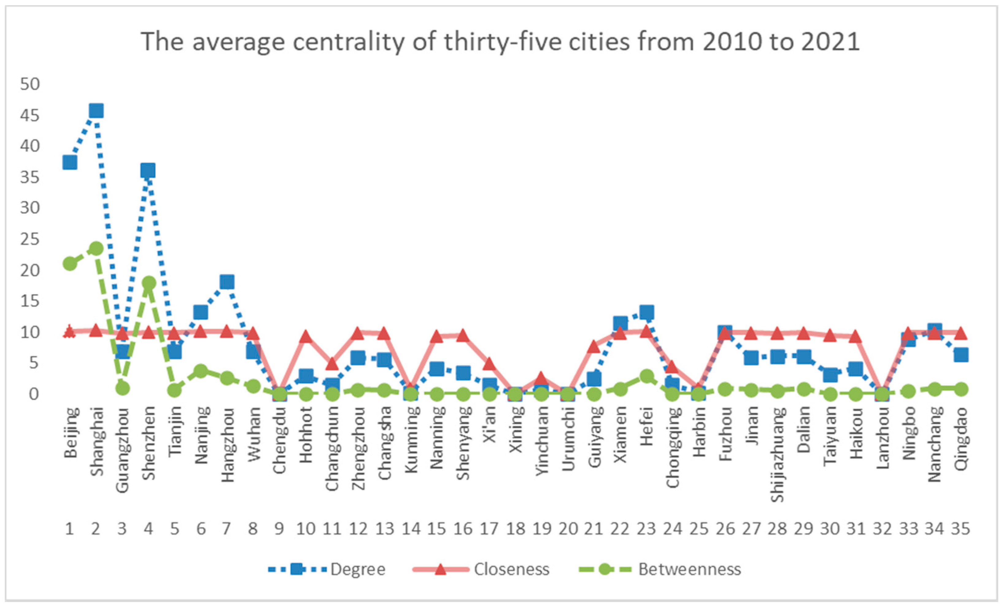
According to the results in Figure 1, there are significant differences in the degree centrality of thirty-five large and medium-sized cities from 2010–2021, among which cities with higher degree of centrality are Beijing, Shanghai, Shenzhen, Nanjing, Hangzhou, Xiamen, and Hefei. The average degree centrality values of housing prices in these cities range from [11.52, 45.83], which are at the core position of the housing price network and have a greater influence on other cities. Some cities have zero degree centrality, indicating that the influence of the city on other cities is weak and negligible, and these cities are isolated from the network. Except for the above cities, the degree centrality of other cities is low, which indicates that although these cities influence other cities, their housing price is still affected by the cities with higher degree centrality and are in a subordinate position.

4.3.2. Closeness Centrality

As can be seen from Figure 1, the average closeness centrality of most cities is within the range of [2,11], only Chengdu, Xining, Kunming, Urumqi, and Lanzhou have been close to zero, which indicates that the housing prices of these cities have a weak attraction relationship with housing prices of other cities. The result is consistent with the findings of degree centrality. The value of closeness centrality indicates that these cities have more or less influence on each other. The larger the value, the broader the influence.

4.3.3. Betweenness Centrality

Observing Figure 1, it can be found that the overall trend of the average betweenness centrality is consistent with the degree centrality. Only a few cities have higher values of betweenness centrality, such as Beijing, Shanghai, Shenzhen, Nanjing, Hangzhou, and Hefei. While other cities have lower or zero values. The above higher betweenness centrality cities also have a high degree centrality, which indicates that the housing prices of the above cities are not only at the core position of the housing price network, but also are the controller of the regional housing prices, and plays a broker role in the network, connect the core and marginal cities.

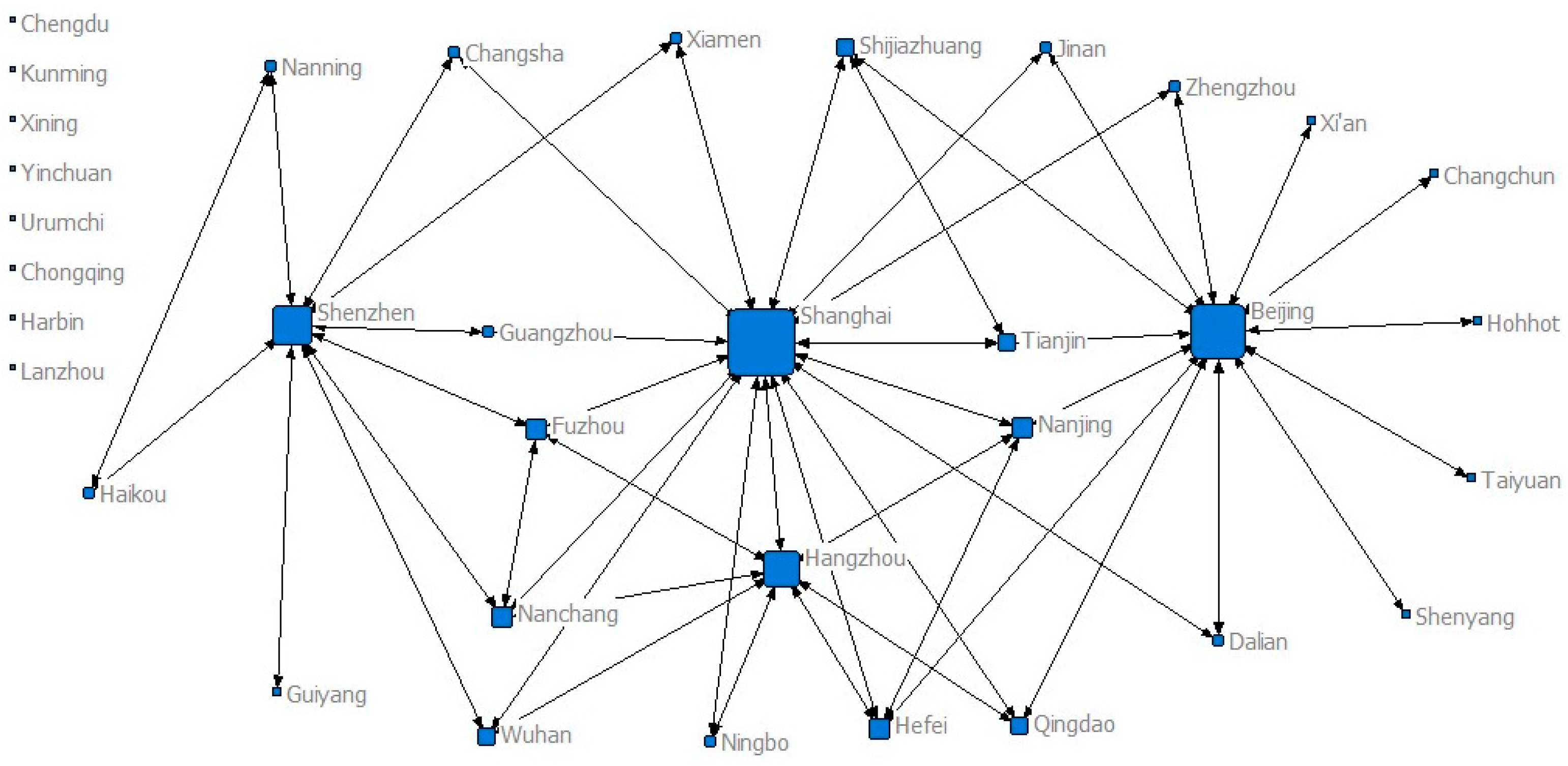
4.4. Network Diagram

From the changes in the overall network structure in Table 4, it can be found that housing price network structure in 2011 deferred significantly from 2013. Followed by a general increase in urban housing prices in 2013 and then a divergence in housing prices, some changes in housing price network structure also occurred after 2016. There is more variability in the performance of the housing price network in these years. In 2020, the economic development and housing markets of all cities are affected by the outbreak of COVID-19, but the density of the housing price network becomes tighter, which is very interesting. Therefore, in order to simplify the analysis, this paper selects network diagrams from 2011, 2013, 2016, and 2020 for presentation (Figure 2, Figure 3, Figure 4 and Figure 5).

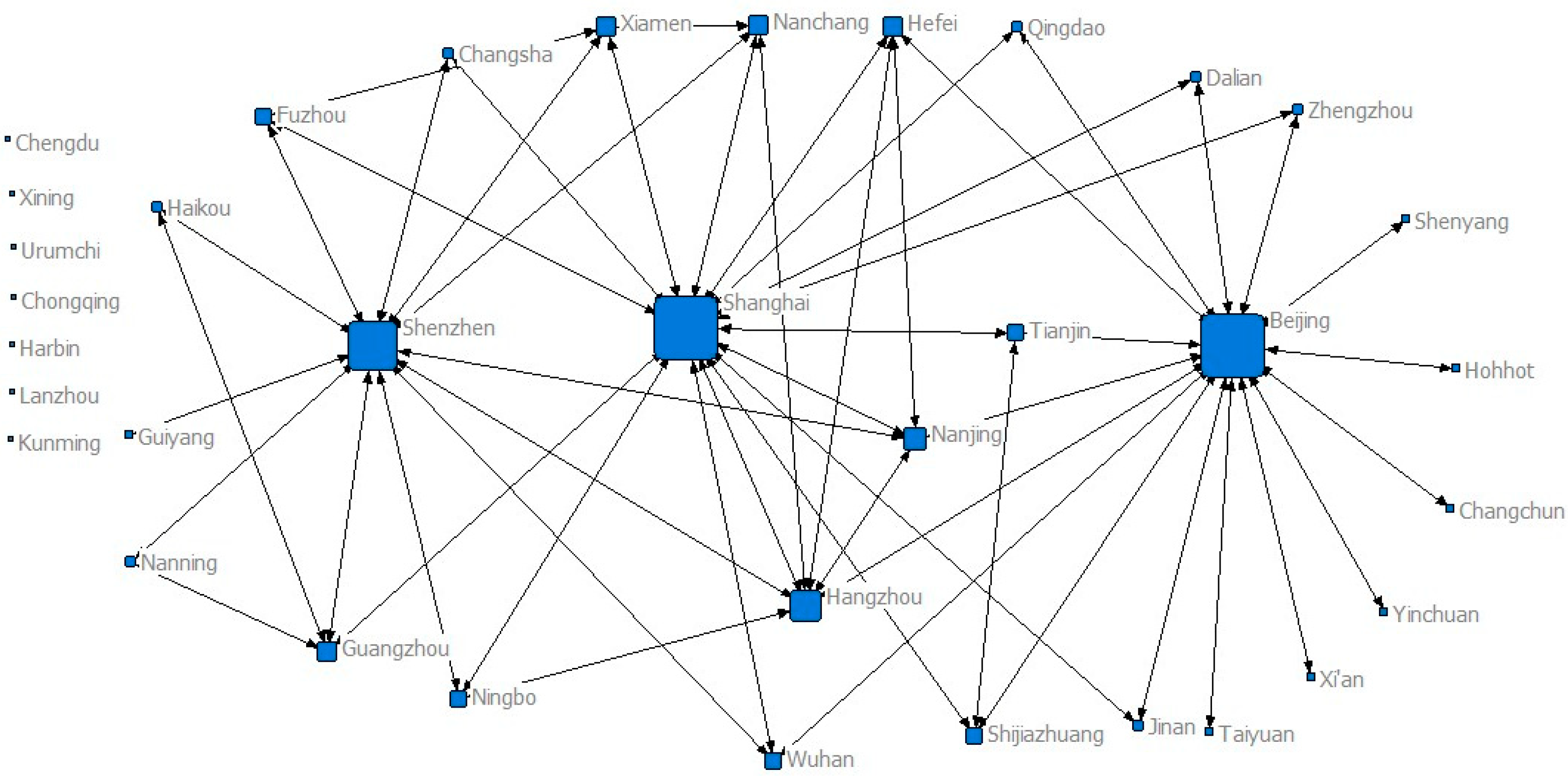
As can be seen from the figure below, the degree of centrality has different performance in these four years, but there are still some certain rules. For example, the three cities of Beijing, Shanghai, and Shenzhen are at the core position and have a high degree centrality in the network diagram every year. While Chengdu and Kunming are located in the southwest of China, and Xining, Urumqi, and Lanzhou are located in the northwest of China, they became less attractive compared to other cities over the years. They are isolated due to the gravity criterion of the relationship set in the SNA. In the network diagram, except for the first-tier cities with greater urban competitiveness, the correlation between the housing prices of other cities has changed over time. Compared with 2011, the number of relationships among urban housing prices in the network increased significantly with Yinchuan joining the housing price network in 2013, and the network became more closely related.

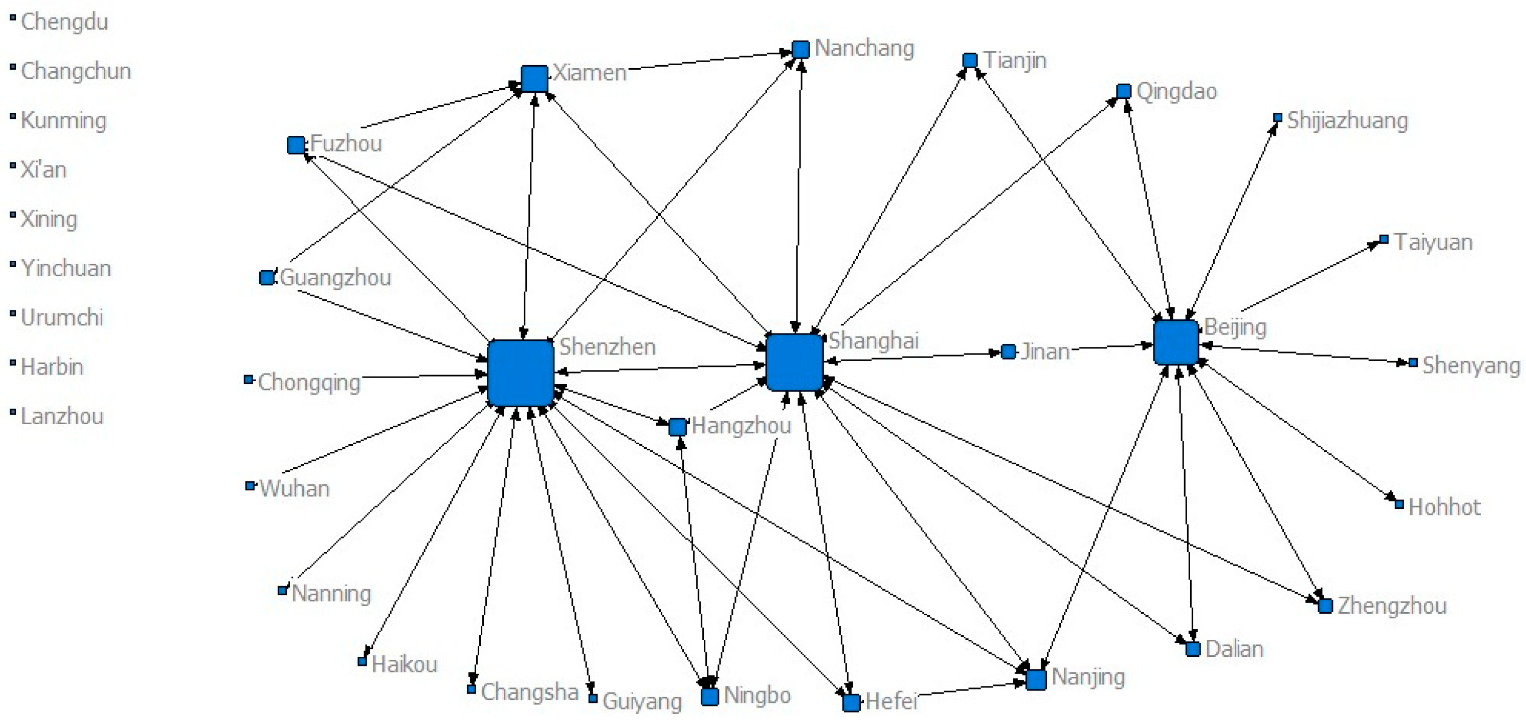
In 2016, the relationships among urban housing prices in the network decreased significantly, and the number of isolated cities increased. Changchun, Xi’an, and Yinchuan became isolated cities. The connection between Chongqing housing prices and the housing price of other cities increased and became non-isolated city. The core position of Hangzhou weakened, this is also consistent with the results of the overall network structure analysis.

Compared with 2016, the number of relationships in the housing price network increased significantly in 2020. Although the housing market was affected by COVID-19 in the early 2020s, this effect is greater for smaller cities, and only individual large and medium-sized cities are affected to some extent, such as Urumqi, Tianjin, Jinan, and Qingdao. These cities where emerging industries are underdeveloped, or where there was a large supply of housing in the early part of the year, had slightly lower or stagnant housing prices. With the proper response to COVID-19 in China, the urban economy is the first to recover among global cities. In particular, in some mega-cities, their housing prices were not greatly affected by the COVID-19, but instead, the backlog of housing demand was gradually released as the economy and society further recovered. For example, Shenzhen’s housing price hits a new high in 2020. Because of the closer relationship with Shenzhen’s housing prices, Guangzhou’s housing prices also began to rise simultaneously, and after a while, Shanghai which is also the metropolis began to rise in housing prices. It directly affected the changes in housing price network.

This study further lists the isolated cities in the housing price network in 2010–2021.

Table 5. The analysis of isolated cities in 2010–2021.

Year	Chengdu	Kunming	Xining	Urumqi	Lanzhou	Chongqing	Harbin	Yinchuan	Changchun	Xi’an	Guiyang
2010	√	√	√	√	√	√	√	◎	◎	◎	◎
2011	√	√	√	√	√	√	√	√	◎	◎	◎
2012	√	√	√	√	√	√	√	√	◎	◎	◎
2013	√	√	√	√	√	√	√	◎	◎	◎	◎
2014	√	√	√	√	√	√	◎	◎	◎	◎	√
2015	√	√	√	√	√	√	√	√	◎	◎	◎
2016	√	√	√	√	√	◎	√	√	√	√	◎
2017	√	√	√	√	√	◎	√	√	√	√	√
2018	√	√	√	√	√	◎	√	√	√	√	◎
2019	√	◎	√	√	√	◎	√	√	√	√	◎
2020	√	√	√	√	√	◎	√	√	√	√	◎
2021	√	√	√	√	√	◎	√	√	√	√	◎

Note: the √ indicates that the city is isolated this year, and the ◎ indicates that the city has been added to the housing price network this year.

shows that Chengdu, Xining, Urumqi, and Lanzhou were isolated over the years. The relationship between housing prices in the above cities and housing price in other cities is also weak, which is also consistent with the finding of individual network structure analysis. This is also in line with the view of the literature [26] and is not considered in other studies.

4.5. Core-Margin Analysis

The importance of each city in the network can be measured by the core-margin analysis. As shown in

Table 6. Core-margin analysis of thirty-five large and medium-sized cities in China.

Year	Beijing	Shanghai	Guangzhou	Shenzhen	Tianjin	Nanjing	Hangzhou	Xiamen	Hefei	Fuzhou	Wuhan
2010	▲	▲	◇	▲	▲	▲	▲	▲	▲	▲	▲
2011	▲	▲	▲	▲	▲	▲	▲	◇	▲	▲	▲
2012	▲	▲	▲	▲	▲	▲	▲	◇	▲	▲	▲
2013	▲	▲	▲	▲	▲	▲	▲	▲	▲	◇	◇
2014	▲	▲	▲	▲	▲	▲	▲	▲	▲	◇	◇
2015	▲	▲	▲	▲	▲	▲	▲	▲	▲	◇	◇
2016	▲	▲	▲	▲	▲	▲	▲	▲	▲	▲	◇
2017	▲	▲	◇	▲	◇	▲	▲	▲	▲	◇	◇
2018	▲	▲	◇	▲	◇	▲	▲	▲	▲	◇	◇
2019	▲	▲	◇	▲	◇	▲	▲	◇	▲	◇	◇
2020	▲	▲	▲	▲	▲	▲	▲	▲	▲	◇	◇
2021	▲	▲	▲	▲	▲	▲	▲	▲	▲	◇	◇

Note: the ▲ indicates that the city is at the core position in the year, and the ◇ indicates that the city is in the marginal position in the year. Cities not listed have been marginal over the years.

, some cities have been at the core position of the network for many years, including Beijing, Shanghai, Shenzhen, Nanjing, Hangzhou, and Hefei. The above six cities can be roughly divided into three types of regions: the region of Beijing, the region of Shenzhen, and the provincial capital cities in the Yangtze River Delta region, all of which have a high level of economic development. Guangzhou, Tianjin, Xiamen, Fuzhou, and Wuhan have also been at the core position, but there are still some fluctuations that put them in a marginal position. Except for isolated cities, the remaining cities, have been on the margin of the housing price network over the years.

Through the analysis of the geographical location and economic development of core-margin cities, it can be found that most of the cities at the margin position are underdeveloped areas, with a lower level of economic development and housing prices. In contrast, most of the cities at the core position are first-tier cities, which have a higher level of economic development, stronger comprehensive strength, and better regional advantages, thus the proportion of housing investment is relatively large and have a profound impact on the prices of the surrounding housing market. These cities can also drive the entire housing market [48]. Therefore, the changes in housing prices of core cities have important reference significance for neighboring cities.

4.6. Cohesive Subgroup Analysis

When the study sets the max depth of splits to 2 and the convergence criteria to 0.2 it can be seen from

Table A1. Spatial spillovers among thirty-five large and medium-sized cities in China in 2011.

Block	The Number of Overflow Relationships in the Block	The Number of Overflow Relationships Outside the Block	The Expected Ratio of Internal Relationships (%)	The Actual Ratio of Internal Relationships (%)	The Name of Block	Image Matrix
						Block 1	Block 2	Block 3	Block 4
Block 1	10	8	19.23	55.56	Beneficial	1	1	0	0
Block 2	4	19	26.92	17.39	Broker	1	0	1	0
Block 3	2	31	7.69	6.06	Spillover	0	1	1	1
Block 4	4	20	34.62	16.67	Bidirectional spillover	0	0	1	0

,

Table A2. Spatial spillovers among thirty-five large and medium-sized cities in China in 2013.

Block	The Number of Overflow Relationships in the Block	The Number of Overflow Relationships Outside the Block	The Expected Ratio of Internal Relationships (%)	The Actual Ratio of Internal Relationships (%)	The Name of Block	Image Matrix
						Block 1	Block 2	Block 3	Block 4
Block 1	12	10	22.22	54.55	Beneficial	1	1	0	0
Block 2	8	25	33.33	24.24	Broker	1	0	1	0
Block 3	0	28	3.70	0.00	Spillover	0	1	0	1
Block 4	8	17	29.63	0.32	Bidirectional spillover	0	0	1	1

,

Table A3. Spatial spillovers among thirty-five large and medium-sized cities in China in 2016.

Block	The Number of Overflow Relationships in the Block	The Number of Overflow Relationships Outside the Block	The Expected Ratio of Internal Relationships (%)	The Actual Ratio of Internal Relationships (%)	The Name of Block	Image Matrix
						Block 1	Block 2	Block 3	Block 4
Block 1	0	10	0.00	0.00	Spillover	0	1	0	0
Block 2	0	18	36.00	0.00	Spillover	1	0	1	0
Block 3	18	21	16.00	46.15	Bidirectional spillover	0	1	1	1
Block 4	2	15	36.00	11.76	Broker	0	0	1	0

and

Table A4. Spatial spillovers among thirty-five large and medium-sized cities in China in 2020.

Block	The Number of Overflow Relationships in the Block	The Number of Overflow Relationships Outside the Block	The Expected Ratio of Internal Relationships (%)	The Actual Ratio of Internal Relationships (%)	The Name of Block	Image Matrix
						Block 1	Block 2	Block 3	Block 4
Block 1	0	41	5.88	0.00	Spillover	0	0	1	1
Block 2	0	0	0.00	0.00	-	0	0	0	0
Block 3	10	22	26.47	31.25	Bidirectional spillover	1	0	0	0
Block 4	2	23	5.88	8.00	Bidirectional spillover	1	0	0	0

in Appendix A, the block model divides the large and medium-sized cities into four blocks—Spillover block, Broker block, Bidirectional Spillover Block, and the Beneficial Block—in 2011 and 2013. There were three types of blocks, two spillover blocks, one broker block, and one bidirectional spillover block, in 2016. There were only two types of blocks, one spillover block and two bidirectional spillover blocks, in 2020.

In 2011 and 2013, Block 2 played the role of broker. Block 1 has a relatively high internal influence, which is in line with the findings of the network diagram analysis. Looking at the magic matrix for 2016, we can see that the number of relationships within the blocks is less than in 2013 and only one of the values of main diagonals is 1. This means that the tightness of the housing price network was lower in 2016, the intra-block linkages of housing price weakened and the inter-block linkages of housing price increased than in previous years.

Compared with the other years, the image matrix changed more in 2020, all the values of the main diagonal are 0. The Spillover Block is connected to the Bidirectional Spillover Block, and there is no connection between two Bidirectional Spillover Blocks. This phenomenon indicates that the urban housing price network has changed a lot, there is a relationship between house prices in different block cities and a weaker relationship between housing prices in the same type of block cities, but a stronger relationship between housing prices in cities inside each block. The reason for this phenomenon may be that the structural divergence of housing prices has become more obvious under the impact of COVID-19, with population and industries further converging to cities with stronger competitiveness and higher quality of public services, or to metropolitan areas and urban agglomeration. Housing prices in these cities continue to rise, while housing prices in other types of cities are relatively depressed.

This paper presents the changes of cities within each block in the main years (

Table 7. The block of thirty-five large and medium-sized cities (except isolated cities).

Year	Spillover Block	Beneficial Block	Broker Block	Bidirectional Spillover Block
2011	Shenzhen Shanghai Hangzhou	Beijing, Xi’an, Hohhot, Changchun, Taiyuan, Shenyang	Nanjing, Jinan, Qingdao, Dalian, Tianjin, Zhengzhou, Hefei, Shijiazhuang	Nanning, Changsha, Guiyang, Xiamen, Fuzhou, Wuhan, Guangzhou, Haikou, Ningbo, Nanchang
2013	Shenzhen Shanghai	Beijing, Xi’an, Yinchuan, Changchun, Shenyang, Hohhot, Taiyuan	Tianjin, Hangzhou, Hefei, Nanjing, Zhengzhou, Shijiazhuang, Jinan, Qingdao, Dalian, Wuhan	Guangzhou, Xiamen, Fuzhou, Guiyang, Nanning, Changsha, Nanchang, Haikou, Ningbo
2016	Beijing, Dalia, Hohhot, Zhengzhou, Tianjin, Nanjing, Jinan, Shijiazhuang, Qingdao, Taiyuan, Shenyang	-	Changsha, Guiyang, Chongqing, Guangzhou, Wuhan, Hefei, Nanning, Haikou, Ningbo, Hangzhou	Xiamen, Shanghai, Nanchang, Fuzhou, Shenzhen
2020	Shenzhen Shanghai Beijing	-	-	Nanning, Changsha, Xiamen, Chongqing, Fuzhou, Guiyang, Wuhan, Guangzhou, Haikou, Ningbo, Nanchang, Hangzhou, Dalian, Hefei, Zhengzhou, Tianjin, Nanjing, Shijiazhuang, Qingdao, Hohhot, Taiyuan, Shenyang, Jinan

). The changing roles of the members within each block are further explored based on the data from the cohesive subgroup analysis. We can find an interesting phenomenon that Shenzhen and Shanghai was a member of Spillover Block in both 2011 and 2013, but Beijing, a first-tier city, was in the Beneficiary Block in these two years. The reason maybe is that Beijing is in the first block in 2011 and 2013, and the number of internal relationships in the block is larger than the external relationships in the block, so it cannot play a “Spillover” role in the whole network. Moreover, Block 1 only has ties with Block 2, and has no ties with other cities in Blocks 3 and 4, and cannot play the role of “Bidirectional Spillover” or “Broker”. During this period, Beijing only had a strong influence on the housing price in cities such as Hohhot and Taiyuan in North China, Changchun and Shenyang in Northeast China, and Xi’an in Northwest China, and had a weaker influence on South and Southwest China.

In 2016, not only Beijing was added to the Spillover Block, but also Dalian, Hohhot, Zhengzhou, Tianjin, Jinan, Shijiazhuang, Qingdao, Taiyuan and Shenyang were added. The reason for this phenomenon is that most of the cities in Block 2 are located in northern China and there is no spillover relationship within the block, but they have a close relationship with cities in southern, eastern and central China in Block 3. Therefore, Block 2 shows a spillover effect. Shanghai and Shenzhen turn to the Bidirectional Spillover Block from the Spillover Block. This means that the housing prices in Shanghai and Shenzhen are not only more connected to the cities in the block, but also linked to the cities outside its block, such as Tianjin, Nanjing, Hangzhou, Zhengzhou, Hefei, Ji’nan, Dalian, Ningbo, and Qingdao; and Shenzhen is connected with eleven cities outside the block, including Guangzhou, Nanjing, Hangzhou, Wuhan, Changsha, Nanning, Guiyang, Hefei, Chongqing, Haikou, and Ningbo.

In 2020, for the first time, the beneficial and broker blocks have no one cities under the impact of COVID-19, indicating that the urban housing price network was hit by this public health emergency (Table 7). Most of the cities located in the northeastern and northern regions originally played an increasingly important role in the housing network, and these cities are no longer only influenced by other cities, but also started to gradually influence other cities. Beijing, Shanghai and Shenzhen became members of the spillover block, housing prices in these cities have a stronger driving and attracting effect on other cities. Most of the cities located in the northeast and northern regions were no longer only influenced by other cities, but also began to gradually influence other cities, and some cities originally in the beneficiary block gradually played a “bidirectional spillover” role. The relationship between housing prices in various cities has become closer, and the whole housing price network tends to be more structurally differentiated.

5. Discussion

Generally, these cities located in the center of the housing price network are first-tier cities, which have a higher housing price base, stronger population siphon effect, and faster economic development than other cities. Therefore, they have a prominent impact on housing prices of other cities and generally belong to the Spillover Block or the Bidirectional Spillover Block. The impact of urban agglomeration development strategy on China’s housing price is also evident. In the Yangtze River Delta urban agglomeration, the second-tier cities, such as Nanjing, Hangzhou and Hefei, also occupy the core position. Most cities belong to the Broker Block or Bidirectional Spillover Block, connecting the first-tier cities, the second and third-tier cities in the housing price network. These cities have more interaction include the transmission of policy information, the flow of population, the exchange of trade activities and other factors, which directly affect the relationship of housing prices. Sometimes, because of more connection with those cities within their radius or related blocks, some regional single-core cities belong to beneficial blocks, such as Beijing in 2011 and 2013, Xi’an in west China, Taiyuan, Hohhot in central China, Changchun, and Shenyang in northeast China, etc.

A few cities are isolated in the housing price network, and these cities are mostly in the southwest, northwest, and northeast regions. Housing prices of these cities are far away from the radiation of the housing price core cities and are influenced by the supply and demand in the local housing markets, which also is the general rule of housing market development. This phenomenon has increased in recent years. It can be seen that the housing regulation policies based on city-specific have played an important role.

In 2020, the impact of the COVID-19 outbreak led directly to price fluctuations in the housing market, making the network of housing prices more closely linked, but at the same time, there was divergence among different cities. The main reason for this phenomenon is that first-tier cities, with strong development and stable demand, were not affected much by this outbreak; when the outbreak stabilized, second-tier and third-tier cities began to recover gradually after being affected initially.

The attraction of housing price among different cities is inevitable, and the healthy development of the housing market is not to blindly suppress the rise of housing prices, but to control the excessive growth rate of housing prices so that the rise of housing prices is within a reasonable range and coordinated with the level of local economic development.

6. Conclusions and Policy Implications

This paper adopted a modified gravity model and SNA to analysis the complex relationship of housing prices with each other in thirty-five large and medium-sized cities in China from 2010–2021. Compared with previous studies, this study takes into account the impact of housing price gap as well as urban housing price level on the relationship in whole network and judges the strength of interrelationship among urban housing price from the perspective of whole network, which to some extent complements the application of network science in urban housing study and makes the interdependence and attraction between urban housing prices concrete and visual. The main findings are as follows:

Firstly, in line with the finding by Chen and Zhang [35], the rise and fall of housing prices in China’s cities are not only affected by the economic environment and local market, but also by the interaction between cities. For the whole structure of the housing price network, similar to the results of Fang and Pei [44], the network density is not high each year and spatial connections need to be strengthened.

Secondly, since housing prices are still generally more influenced by local supply and demand, the overall structural relationship of the housing price network is not very tight, and it changes from year to year, especially when there is a large sudden external shock or when housing prices in a city suddenly rise or fall.

Finally, each city plays a different role in the network. In addition to the linkage between urban housing prices in intra-block cities, there is also a linkage between urban housing prices inter-block. Those housing prices of the first-tier cities are located at the center of the network and have a great influence on other cities in the housing price network, while some underdeveloped cities in the northwest and southwest have little influence. With the development of regional economic integration, housing prices in some second-tier and third-tier cities also interact and fluctuate together with the entire housing price network.

Therefore, governments at all levels should pay more attention to these cities with a high core position in the whole network and cities with sudden changes in housing prices, take timely measures to prevent and reduce the price contagion phenomenon brought by irrational increases of housing price in some core cities. Local governments should also add to establish a reasonable housing price system that suits local supply and demand according to different socio-economic carrying capacity. The central government should pay attention to monitoring the stability of the housing price network, making regulations and establishing policy directions, and trying to keep the housing price network from fluctuating too much. Central government also should urge local governments to control the growth rate of housing prices and coordinate it with their local economic development.

Certainly, there are some limitations in terms of the gravity model in this study, which can only simulate the possible attraction relationship through the performance of housing prices. It is also a relative result to judge the strength or weakness of the housing price relationship through SNA. However, and even so, this study can be useful in exploring inter-city housing price relationships from a networked perspective and how to better integrate the overall national house price regulation guidelines and implement local city-specific policies.

References

- Short, J.R. Black holes and loose connections in a global urban network. Prof. Geogr. 2004, 56, 295–302. [Google Scholar]
- Meen, G. Spatial aggregation, spatial dependence and predictability in the UK housing market. Hous. Stud. 1996, 11, 345–372. [Google Scholar] [CrossRef]
- Holly, S.; Pesaran, M.H.; Yamagata, T. A spatio-temporal model of house prices in the USA. J. Econom. 2010, 158, 160–173. [Google Scholar] [CrossRef]
- Chen, M.L.; Liu, H.J.; Sun, Y.N.; He, L.W. Empirical study on the characteristics of network structure and its influence factors of urban housing price linkage: Based on monthly data of 69 large and medium cities in China. S. China. J. Econ. 2016, 34, 71–88. (In Chinese) [Google Scholar]
- Lv, L.; Liu, H.Y. Research on the measurement, network structure and influencing factors of the spillover effect of urban housing prices. Econ. Rev. 2019, 2, 125–139. (In Chinese) [Google Scholar]
- Albert, R.; Barabasi, A.L. Dynamics of complex systems: Scaling laws for the period of Boolean networks. Phys. Rev. Lett. 2000, 84, 5660–5663. [Google Scholar] [CrossRef] [PubMed] [Green Version]
- Qiao, S.J.; Han, N.; Gao, Y.J.; Li, R.H.; Huang, J.B.; Guo, J.; Gutierrez, L.A.; Wu, X.D. A fast parallel community discovery model on complex networks through approximate optimization. IEEE Trans. Knowl. Data Eng. 2018, 30, 1638–1651. [Google Scholar] [CrossRef]
- Pow, J.; Gayen, K.; Elliott, L.; Raeside, R. Understanding complex interactions using social network analysis. J. Clin. Nurs. 2012, 21, 2772–2779. [Google Scholar] [CrossRef]
- Smith, D.A.; Timberlake, M.F. World city networks and hierarchies, 1977–1997—An empirical analysis of global air travel links. Am. Behav. Sci. 2001, 44, 1656–1678. [Google Scholar] [CrossRef]
- Manchin, M.; Orazbayev, S. Social networks and the intention to migrate. World Dev. 2018, 109, 360–374. [Google Scholar] [CrossRef] [Green Version]
- Liu, W.; Xu, J.; Li, J. The influence of poverty alleviation resettlement on rural household livelihood vulnerability in the western mountainous areas, China. Sustainability 2018, 10, 2793. [Google Scholar] [CrossRef] [Green Version]
- Drake, L. Testing for convergence between UK regional house prices. Reg. Stud. 1995, 29, 357–366. [Google Scholar] [CrossRef]
- Meen, G. Regional house prices and the ripple effect: A new interpretation. Hous. Stud. 1999, 14, 733–753. [Google Scholar] [CrossRef]
- Clapp, J.M.; Tirtiroglu, D. Positive feedback trading and diffusion of asset price changes: Evidence from housing transactions. J. Econ. Behav. Organ. 1994, 24, 337–355. [Google Scholar] [CrossRef]
- Holly, S.; Pesaran, M.H.; Yamagata, T. The spatial and temporal diffusion of house prices in the UK. J. Urban Econ. 2011, 69, 2–23. [Google Scholar] [CrossRef] [Green Version]
- Miao, H.; Ramchander, S.; Simpson, M.W. Return and volatility transmission in U.S. housing markets. Real Estate Econ. 2011, 39, 701–741. [Google Scholar] [CrossRef]
- Teye, A.L.; Knoppel, M.; de Haan, J.; Elsinga, M.G. Amsterdam house price ripple effects in the Netherlands. J. Eur. Real Est. Res. 2017, 10, 331–345. [Google Scholar] [CrossRef] [Green Version]
- Hudson, C.; Hudson, J.; Morley, B. Differing house price linkages across UK regions: A multi-dimensional recursive ripple model. Urban Stud. 2018, 55, 1636–1654. [Google Scholar] [CrossRef]
- Gupta, R.; Miller, S.M. “Ripple effects” and forecasting home prices in Los Angeles, Las Vegas, and Phoenix. Ann. Reg. Sci. 2012, 48, 763–782. [Google Scholar] [CrossRef] [Green Version]
- Grigoryeva, I.; Ley, D. The price ripple effect in the Vancouver housing market. Urban Geogr. 2019, 40, 1168–1190. [Google Scholar] [CrossRef]
- Liu, Z.P.; Chen, Z.P. Spatial correlation, influencing factors and pass-through effect of urban housing prices: An empirical research based on regional market relation. J. Shanghai Univ. Fin. Econ. 2013, 15, 81–88. (In Chinese) [Google Scholar]
- Wang, X.; Hang, Y.H.; Wang, C. Measurement of connectedness and spillovers in China’s housing market: Based on the DAG and spillover index model. J. Appl. Stat. Manag. 2018, 37, 713–727. (In Chinese) [Google Scholar]
- Zhou, Q.W.; Den, X.P.; Chang, T.Y. Empirical research on space-time linkage of residential price between regional cities based on ripple-spillover effect: Taking Nanjing metropolitan area as an example. Constr. Econ. 2018, 39, 66–70. (In Chinese) [Google Scholar]
- Hong, T.; Xi, B.; Gao, B. Co-movement of real estate prices and spatial diffusion of bubbles: Evidence from 35 metropolis in China from 2000 to 2005. Stat. Res. 2007, 24, 64–67. (In Chinese) [Google Scholar]
- Wang, S.T.; Yang, Z.; Liu, H.Y. An empirical study on the interaction of housing prices in regional market cities in China. Res. Fin. Econ. Issues 2008, 6, 122–129. (In Chinese) [Google Scholar]
- Lee, C.C.; Chien, M.S. Empirical modeling of regional house prices and the ripple effect. Urban Stud. 2011, 48, 2029–2047. [Google Scholar] [CrossRef]
- Zhang, X.; Lin, R.D. Empirical study of short-term ripple effect of China’s urban housing price. Fin. Econ. 2015, 9, 132–140. (In Chinese) [Google Scholar]
- Matsumoto, H. International urban systems and air passenger and cargo flows: Some calculations. J. Air Transp. Manag. 2004, 10, 239–247. [Google Scholar] [CrossRef] [Green Version]
- Murat Celik, H.; Guldmann, J.M. Spatial interaction modeling of interregional commodity flows. Socioecon. Plann. Sci. 2007, 41, 147–162. [Google Scholar] [CrossRef] [Green Version]
- Liu, H.J.; Liu, C.M.; Sun, Y.N. Spatial correlation network structure of energy consumption and its effect in China. Chin. Ind. Econ. 2015, 5, 83–95. (In Chinese) [Google Scholar]
- Li, X.T.; Feng, D.; Li, J.; Zhang, Z.S. Research on the spatial network characteristics and synergetic abatement effect of the carbon emissions in Beijing-Tianjin-Hebei urban agglomeration. Sustainability 2019, 11, 1444. [Google Scholar] [CrossRef] [Green Version]
- Song, J.Z.; Feng, Q.; Wang, X.P.; Fu, H.L.; Jiang, W.; Chen, B.Y. Spatial association and effect evaluation of CO2 emission in the Chengdu-Chongqing urban agglomeration: Quantitative evidence from social network analysis. Sustainability 2019, 11, 1. [Google Scholar] [CrossRef] [Green Version]
- Zeng, Z.; Qiu, D.C.; Li, F.; Li, X.G.; He, Y. Suitability evaluation on the spatial layout of the public rental housing based on the gravity model: Taking nine districts of Chongqing as an example. China Land Sci. 2014, 28, 52–59. (In Chinese) [Google Scholar]
- Mao, F.F.; Wang, J.S. Can indemnificatory housing promote population flow?—A gravity model analysis based on the inter-provincial population flow. East China Econ. Manag. 2016, 30, 86–95. (In Chinese) [Google Scholar]
- Chen, L.F.; Zhang, F.Q. Study on the ripple effect of housing price under the coordinated development of Beijing-Tianjin-Hebei region. Price Theor. Pract. 2018, 8, 139–142. (In Chinese) [Google Scholar]
- Li, R. Spatial scope estimation of Shenzhen metropolitan area based on expanded gravity model of residential connection. Spec. Zone Econ. 2019, 10, 49–51. (In Chinese) [Google Scholar]
- Barnes, J.A. Class and committees in a Norwegian island parish. Hum. Relat. 1954, 7, 39–58. [Google Scholar] [CrossRef]
- Becker, G.S. A theory of social interactions. J. Polit. Econ. 1974, 82, 1063–1093. [Google Scholar] [CrossRef]
- Tindall, D.B.; Wellman, B. Canada as social structure: Social network analysis and Canadian sociology. Can. J. Sociol. Cah. Can. Sociol. 2001, 26, 265–308. [Google Scholar] [CrossRef]
- Yao, Q.; Ma, H.; Yan, H.; Chen, Q. Analysis of social network users online behavior from the perspective of psychology. Adv. Psych. Sci. 2014, 22, 1647–1659. [Google Scholar] [CrossRef]
- Ghafouri, H.B.; Mohammadhassanzadeh, H.; Shokraneh, F.; Vakilian, M.; Farahmand, S. Social network analysis of Iranian researchers on emergency medicine: A sociogram analysis. Emerg. Med. J. 2014, 31, 619–624. [Google Scholar] [CrossRef] [PubMed]
- Boegenhold, D. Social network analysis and the sociology of economics: Filling a blind spot with the idea of social embeddedness. Am. J. Econ. Sociol. 2013, 72, 293–318. [Google Scholar] [CrossRef] [Green Version]
- Prell, C.; Hubacek, K.; Reed, M. Stakeholder analysis and social network analysis in natural resource management. Soc. Nat. Resour. 2009, 22, 501–518. [Google Scholar] [CrossRef]
- Fang, D.C.; Pei, M.D. The empirical analysis of the spatial correlation network structure of housing price. Shanghai J. Econ. 2018, 1, 63–73. (In Chinese) [Google Scholar]
- Wang, Q.H.; Cheng, L.F.; Zhang, F.Q. Research on the network structure of housing price interaction in Beijing-Tianjin-Hebei region. Areal Res. Devel. 2019, 38, 51–56. (In Chinese) [Google Scholar]
- Ma, S.Z.; Ren, W.W.; Wu, G.J. The characteristics of a country’s agricultural trade network and its impact on global value chain division: Based on social network analysis. Manag. World 2016, 3, 60–72. (In Chinese) [Google Scholar]
- Jin, H.; Jia, Y.; Qian, Z.F. Visual analysis on research development of knowledge sharing in virtual community by using social network analysis. Oper. Res. Manag. Sci. 2017, 26, 149–157. (In Chinese) [Google Scholar]
- Zhang, L.; Wang, H.; Song, Y.; Wen, H.Z. Spatial spillover of house prices: An empirical study of the Yangtze Delta urban agglomeration in China. Sustainability 2019, 11, 544. [Google Scholar] [CrossRef] [Green Version]
Figure 1.
The average centrality of thirty-five cities from 2010 to 2021.
Figure 2.
Network diagram of degree centrality in 2011.
Figure 3.
Network diagram of degree centrality in 2013.
Figure 4.
Network diagram of degree centrality in 2016.
Figure 5.
Network diagram of degree centrality in 2020.