Implementing Horizontal Cooperation in Public Transport and Parcel Deliveries: The Cooperative Share-A-Ride Problem

Abstract

The static share-a-ride problem (SARP) consists of handling people and parcels in an integrated way through the same vehicle, which provides a shared trip between an origin and a destination, in response to requests received in advance. When multiple providers compete on the same market (for instance, within the same city or region), horizontal cooperation can be an efficient strategy to consolidate all requests and to optimize the total payoff. This situation gives rise to the cooperative SARP (coop-SARP). In this problem, multiple depots and heterogeneous vehicles must be considered and different cooperation levels may be agreed upon by service providers. In this paper, we propose a new mathematical programming formulation for cooperative SARP along with theoretical bounds. Moreover, through numerical experiments and ad hoc statistics, we analyze the benefits of different levels of horizontal cooperation between service providers. The results show that cooperation leads to reduced travel times and to improved vehicle occupancy rates, service levels, and profits, which make such a cooperative system even more appealing for service providers.

1. Introduction

Nowadays, populations, cities, economies, and trade are significantly growing, and they are expected to increase even further in the next years. As a consequence, urbanization and demands for goods and services are increasing. In addition, the digital revolution and recent technological advances have contributed to the growth of the e-commerce industry, for which speed and timeliness of delivery are fundamental [1,2]. While these trends are creating new opportunities, they are unavoidably leading to some emerging challenges. Specifically, the increased freight and passenger activity within the urban area results in road congestion, air and noise pollution, traffic accidents, greenhouse gas emissions, and energy consumption [3,4]. The recent National (USA) Household Travel survey [5] highlighted that, in 2017, the average car occupancy rate showed a stable trend of $1.67$ passengers per car. Furthermore, typically, within the city, people and freight transportation are handled separately. These two behaviors contribute to the presence of a large number of vehicles on the road.

In this context, optimal delivery planning is crucial (see, Guerlain et al. [6] and Macioszek [7] for an overview of the available approaches and tools) and new city logistic systems based on more sustainable approaches are becoming more and more popular. Among these, key roles are played by ride-sharing, by the integration of people and parcel delivery, and by on-demand public transportation services. All three approaches contribute to the increase in efficiency and efficacy of people and freight flow management within the city, encouraging higher vehicle occupancy rates, which, in turn, reduce the number of freight and passenger movements, and air and noise pollution.

Ride-sharing allows passengers to share travel costs and drivers and serves more requests simultaneously, so that both benefit from shared rides. Furthermore, the presence of multiple passengers allows people to reach their destination faster because the driver can often travel along high-occupancy lanes, which are reserved for vehicles carrying more than two passengers [8].

However, the term “sharing” refers to not only “sharing with people” but also “sharing with freight”. This practice is common for long-haul transportation [9], where service providers, such as Norwegian Hurtigruten, carry freight and people at the same time. Nevertheless, for short-haul transportation, people and freight are typically assigned to separated vehicles, even if they frequently share the same infrastructure [10]. The integration of passengers and parcels fosters the use of spare capacity in public transport systems and of idle times to deliver parcels. A pioneer service provider is Connexxion.nl, which delivers both people and parcels in the Netherlands.

Concerning on-demand public transportation services, for passengers, the absence of fixed routes and schedules provides more flexibility and shorter service times due to the absence of mandatory stops. As a result, these transportation services are more flexible and quicker than a bus and cheaper than a taxi. On the freight transportation side, parcels can be picked up and delivered directly at customers’ locations and, provided that the used vehicles are small and comply with the environmental requirements (CO₂ emissions and noise), they are not subject to accessibility restrictions, which usually affect trucks in some neighborhoods. Moreover, from the administration point of view, these transportation services stimulate the level of service, especially for regions characterized by a particular topography or by low demand.

In the last decade, the sharing economy principles have shown their potential not only from the environmental point of view but also in increasing the profits of service providers that embrace those principles. This is particularly true in transportation, where the topic of cooperating service providers has given rise to a huge interest in the last years, as assessed in recent surveys on cooperative urban transportation modes by Cleophas et al. [11] and Mourad et al. [12]. In these papers, hundreds of examples of cooperation modes in logistics are presented. In the authors’ view, when cooperating, stakeholders increase their efficiency by sharing resources and, at the same time, by producing less pollution and by lowering prices for goods. In particular, in cities with many competing transportation service providers, horizontal cooperation results in huge savings for service providers (due to the reduction routing costs), in the increase in service quality (as more transportation requests can be satisfied), and in a significant reduction in city pollution. The literature points out that cooperation in city logistics could be very challenging because planning and control of the system has to be well calibrated. In particular, guarantees in future profits have to be given to enhance the compliance of competing service providers to the coalitions.

All these features are included in the cooperative share-a-ride problem (coop-SARP) that we introduce. Typically, the SARP consists of handling people and parcels in an integrated way by finding the best schedules and routes and, from the modeling point of view, it is a generalization of the dial-a-ride problem (DARP), where parcels also are considered. The distinguishing features of the SARP proposed by Li et al. [13] are that (i) people and parcel share ride services; (ii) passengers must be served within a hard time window, while parcels are not prioritized; (iii) only one passenger can be carried simultaneously by the vehicle; and (iv) only a predetermined number of parcels can be picked up between a passenger drop on and drop off.

In this paper, we propose the following extension to the classical SARP. In a city, multiple service providers offer on-demand transportation services for people and parcels. With these service providers being different, their depots have different locations and they use heterogeneous vehicles. Users can book their requests in advance (usually within the night before the day in which the service takes place), and their requests are collected and managed by a centralized system, which finds the best routing in terms of the overall payoff, by taking into account multiple constraints, such as pickup and delivery times, the capacity of the vehicles, and the driver shift duration. To make this cooperative scheme fair and to give incentives to service providers to participate, the benefits arising from the coalition are bigger at the aggregate level than those that could be achieved in a noncooperative system. However, determining the optimal redistribution of the rewards is out of the scopes of this paper, and as in Molenbruch et al. [14], we assume the redistribution occurs a posteriori, if needed. Even if the share-a-ride scheme refers to the possibility of transporting people and parcels on the same vehicle, they have different required levels of service. Passengers desire a travel time required to reach their destinations that does not exceed a desired threshold, while parcels have weaker constraints on pickup and delivery times represented by time windows. Consequently, passenger requests have higher priority. Furthermore, we extend the classical SARP by assuming that the number of passengers and parcels that can be simultaneously carried on a vehicle is constrained only by the vehicle capacity in terms of passenger and parcel volumes. Finally, the focus of this work is on the maximization of the system profit and on the enhancement of users’ experience (both for passengers and for parcel shippers and consignees). Concerning the system profit, we impose a reward for each passenger and parcel request that is served, and we charge routing costs for each traveled arc, penalties for deviations from the passenger request desired pickup and/or delivery time, and a lost reward for each request not accepted.

The contributions of this paper are the following. First, we introduce the new cooperative SARP and we propose a mathematical model for it. This new formulation captures more realistic features, such as the presence of multiple service providers, of multiple depots, and of heterogeneous vehicles and the possibility of carrying more passengers and parcels simultaneously. Moreover, the most outstanding contribution of this model is the ability to manage also economic factors by considering different degrees of horizontal cooperation among service providers. These different levels of cooperation arise from different agreements on the percentage of individual profit that each service provider wants to be guaranteed with respect to the one they could achieve in a noncooperative setting. The higher this percentage, the less flexible the cooperation. Second, we derive mathematical properties for the bounds of this new type of problem. Third, we generate specific instances for the coop-SARP that are based on the maps of real metropolitan road networks. Finally, through numerical experiments, we assess the benefits of cooperating both in terms of the whole coalition and at the individual service provider level.

The paper is organized as follows. Section 2 presents a review of the literature connected to the coop-SARP, while in Section 3, the mathematical model is formulated and theoretical properties are derived. Section 4 provides an illustrative example. Section 5 describes how new map-based instances are generated and presents the computational results. Finally, Section 6 presents the conclusions and future research directions.

2. Literature Review

The SARP was proposed for the first time by Li et al. [13]. In their work, the authors provide a description of the problem and present multiple mathematical formulations. In its classical version, the model accounts only for one depot and homogeneous vehicles. Furthermore, the authors do not consider service times or violations of desired pickup and delivery times and they do not model the situation in which the same vehicle serves two passenger requests one after another. Only a limited number of papers have provided extensions to this problem. Li et al. [15] included service times and a penalty for the violation of parcel time windows, and they considered two sources of uncertainty for this problem, which are stochastic travel times and delivery locations. Another extension is the share-a-ride with parcel lockers problem (SARPLP) by Beirigo et al. [16], who considered shared autonomous vehicles (instead of taxis) that carry more passengers and parcels of different types simultaneously.

A common feature of all these papers is an assumption of the presence of a unique service provider, while in real-world applications, there may be multiple service providers offering ride-sharing transportation services within the same area. Our work contributes to filling this gap in the literature in two ways. First, we consider multiple service providers, each one with its own depot and a different vehicle fleet. Second, we ensure that the benefits arising from horizontal cooperation for this problem will be fair for each participant. A pioneer work in this regard is represented by Molenbruch et al. [14], who, through a real-case study, analyzed the benefits arising from the cooperation of service providers for the DARP and identified the reduction in empty trips as the main reason for lower costs.

To the best of our knowledge, no work exists considering horizontal cooperation for the SARP.

Concerning the model formulation, the SARP can be seen as a special case of the DARP. For the sake of completeness, in the following, we also list contributions in the domain of DARP formulations. Cordeau and Laporte [17] reviewed early methodologies and classical DARP models, which inspired further studies related to different applications. Among these, some examples are non-profit DARP for elderly and disable people [18,19,20,21,22], airport shuttle services [23], healthcare services [24,25,26,27,28,29], demand-responsive models for public transportation [30,31,32], and horizontal cooperation among service providers performing dial-a-ride services [14]. Toth and Vigo [33], Ho et al. [34], and Molenbruch et al. [29] surveyed all these DARP variants.

Enlarging the focus to the methodologies used for the DARP, they can be classified in two classes: exact and heuristic algorithms. Because in this paper we are only interested in analyzing exact solutions, our review focuses uniquely on the first class.

Within the exact methods, there are the ones based on the classical Branch and Bound (B&B) paradigm. However, the standard B&B applied to the DARP is very slow to converge and is computationally cumbersome. As a result, more sophisticated techniques have been developed to speed up the computation, such as Branch and Cut (combining B&B and cutting planes techniques; see Cordeau [35], Ropke et al. [36], and Braekers and Kovacs [37]) and Branch and Price (combining B&B with column generation techniques; see Garaix et al. [31] and Feng et al. [38]). In Gschwind and Irnich [39], a combination of Branch and Cut, and Branch and Price is implemented, and up until now, this has been the best performing exact algorithm for the standard DARP. Nevertheless, for this problem, exact techniques solve instances with up to only eight vehicles and 96 requests in reasonable runtimes. For variants of the standard DARP, the maximum size of the instances that can be solved using exact methods is even smaller. Because most real-world problems are much bigger than the maximum solvable size, developing heuristic algorithms could become a necessity.

3. Model Formulation

In this section, we present the mathematical formulation for the coop-SARP.

We represent the set of service providers (i.e., depots) within the city using $\mathcal{M}$, and the set of requests is denoted by $\mathcal{C}$. This set can be defined as $\mathcal{C}\equiv {\cup }_{m\in \mathcal{M}}{\mathcal{C}}_m$, i.e., the union of requests over all service providers, or as $\mathcal{C}\equiv {\mathcal{C}}^p\cup {\mathcal{C}}^f$, i.e., the union of all passenger and parcel requests, respectively. From this notation, it follows that ${\mathcal{C}}_m^p$ represents the passenger requests for service provider m and that ${\mathcal{C}}_m^f$ stands for the parcel requests for service provider m. Each request has an origin point $O_c$, a destination $D_c$, both with their loads standing for the number of passengers or volume units of parcels associated with the request.

The problem can be represented on a complete directed graph $\mathcal{G}\equiv (\mathcal{V},\mathcal{A})$, where $\mathcal{V}\equiv \mathcal{O}\cup \mathcal{D}\cup \mathcal{H}$, with $\mathcal{O}$ standing for the set of all request origins, $\mathcal{D}$ for the respective destinations, and $\mathcal{H}$ for the set of depots. Each service provider m has one depot, each one doubled in two different nodes, namely the depot exit $h_m$ and the depot entry $h_m^{\prime }$, both in $\mathcal{H}$. Each node i is associated with a load $q_i$, such that $q_i=0$ if $i=h_m,h_m^{\prime },m\in \mathcal{M}$; $q_i\ge 0$ if $i\in \mathcal{O}$; and $q_i\le 0$ if $i\in \mathcal{D}$, and it is consistently associated with a service time $s_i$, which is the time required to load or unload a request. If two origins or destinations are both in node i, we double the node to let each node act as an origin or a destination of a specific request. We assume that each parcel request $c\in {\mathcal{C}}^f$ must be satisfied within a time window $[e_i,l_i]$, where $e_i$ and $l_i$ stand for the earliest and the latest times, respectively, while each passenger request $c\in {\mathcal{C}}^p$ has a desired time $U_{O_c}$ for the picking and a desired time $U_{D_c}$ for the delivery operation. Each arc $(i,j)\in \mathcal{A}$ is characterized by a cost $d_{ij}$ and by a travel time $t_{ij}$. We let ${\mathcal{K}}_m$ be the set of vehicles owned by service provider $m\in \mathcal{M}$ and $\mathcal{K}$ is the set of all vehicles, $\mathcal{K}={\bigcup }_{m\in M}{\mathcal{K}}_m$. Each vehicle has a known capacity for passengers $Q_k^p$, a known capacity for parcels $Q_k^f$, and it is led by a fixed driver whose maximum working time per day is denoted by $T_k$.

We let the binary variable $x_{ij}^k$ be equal to one if arc $(i,j)\in \mathcal{A}$ is traversed by vehicle $k\in \mathcal{K}$ and zero otherwise. The binary variable $y_c^k$ is equal to one if request $c\in \mathcal{C}$ is served by vehicle $k\in \mathcal{K}$ (zero otherwise). For our formulation, the binary variables representing outsourced requests are not explicitly declared but the model can be easily extended to accommodate this situation. Furthermore, the integer variable $w_i^k$ represents the load of vehicle $k\in \mathcal{K}$ in terms of passengers after visiting node i, while the integer variable ${\lambda }_i^k$ stands for the load of vehicle $k\in \mathcal{K}$ in terms of parcels after visiting node i. The continuous variables $l_{O_c}^k$ represent the discrepancy between the real serving time and the desired serving time $U_{O_c}$ of origin $O_c$ of the request $c\in C^p$ by vehicle k. Similarly, the continuous variables $l_{D_c}^k$ represent the discrepancy between the real serving time and the desired serving time $U_{D_c}$ for destination $D_c$ of the request $c\in C^p$ by vehicle k. To model times, we introduce two types of continuous variables: $u_i^k$, which represents the time at which vehicle $k\in \mathcal{K}$ starts serving node i, and $r_c^k$, which denotes the ride time of passengers in request $c\in C^p$. For this latter quantity, we impose a maximum ride time ${\overline{r}}_c$ representing the tolerated excess in the passengers’ ride time.

Finally, the objective of our model maximizes the system profit and improves customers’ experience. We consider request-dependent rewards ${\eta }_c$, $c\in {\mathcal{C}}^p\cup {\mathcal{C}}^f$, which are gained for each served passenger and parcel request. If the service providers cannot serve all parcel requests, some of them should be rejected and outsourced to the freight network. While outsourcing costs are not explicitly included in our model, we consider the lost reward for not accepting a request as an opportunity cost for the system and we denote it by ${\rho }_c$. Concerning cost components, we denote the routing cost of arc $(i,j)$ by $d_{ij}$ and a penalty cost $\gamma$ for each time unit deviation of the passenger pickup or delivery time from the desired time, i.e., $U_{O_c}$ and $U_{D_c}$.

Table 1. Sets, parameters, and variables for the coop-share-a-ride problem (SARP) (2)–().

Sets
$\mathcal{M}$	Set of service providers $\mathcal{M}=\{1,\cdots ,m,\cdots ,M\}$
${\mathcal{C}}_m$	Set of requests for each service provider $m\in \mathcal{M}$
${\mathcal{C}}^p$	Set of passenger requests
${\mathcal{C}}^f$	Set of parcel requests
${\mathcal{C}}_m^p$	Set of passenger requests for service provider $m\in \mathcal{M}$
${\mathcal{C}}_m^f$	Set of parcel requests for service provider $m\in \mathcal{M}$
$\mathcal{C}$	Set of requests, $\mathcal{C}\equiv {\cup }_{m\in \mathcal{M}}{C}_m$ or $\mathcal{C}\equiv {\mathcal{C}}^p\cup {\mathcal{C}}^f$
$\mathcal{V}$	Set of vertices, $\mathcal{V}\equiv \mathcal{O}\cup \mathcal{D}\cup \mathcal{H}$
${\mathcal{V}}^p$	Set of vertices that are either the origin or destination of a passenger request
${\mathcal{V}}^f$	Set of vertices that are either the origin or destination of a parcel request
$\mathcal{O}$	Set of request origins
$\mathcal{D}$	Set of request destinations
$\mathcal{H}$	Set of depots, $\mathcal{H}\subseteq \mathcal{V}$, where each depot $h_m\in \mathcal{H}$ has been doubled in $h_m$ and $h_m^{\prime }$
$\mathcal{A}$	Set of arcs
${\mathcal{K}}_m$	Set of vehicles owned by service provider m
$\mathcal{K}$	Set of vehicles, $\mathcal{K}\equiv {\cup }_{m\in \mathcal{M}}{\mathcal{K}}_m$
Parameters
$Q_k^p$	Passenger capacity of vehicle k
$Q_k^f$	Parcel capacity of vehicle k
$T_k$	Maximal route duration for vehicle k
$q_i$	Load of request i
$s_i$	Service time of node i
$[e_i,l_i]$	Time window for parcel request i
$U_{O_c}$	Desired pickup $O_c$ time for passenger request $c\in {\mathcal{C}}^p$
$U_{D_c}$	Desired delivery $D_c$ time for passenger request $c\in {\mathcal{C}}^p$
$t_{ij}$	Travel time between stops i and j
${\overline{r}}_c$	Passenger request c’s maximum ride time
${\eta }_c$	Reward for each served passenger or parcel request c
$d_{ij}$	Routing cost for arc $(i,j)$
$\gamma$	Unit penalty cost for deviations from the passenger request desired pickup or delivery time
${\rho }_c$	Lost reward for not accepting request c (computed as percentage of the request reward)
Variables
$x_{ij}^k$	Binary variable equal to 1 if arc $(i,j)\in \mathcal{A}$ is traversed by vehicle k, 0 otherwise
$y_c$	Binary variable equal to 1 if passenger’s request $c\in {\mathcal{C}}^p$ is served and 0 otherwise
$u_i^k$	Time at which vehicle k starts serving node i
$l_{O_c}^k$	Discrepancy between the real serving time and desired serving time of origin $O_c$ by vehicle k
$l_{D_c}^k$	Discrepancy between the real serving time and desired serving time of origin $D_c$ by vehicle k
$w_i^k$	People load of vehicle k when leaving node i
${\lambda }_i^k$	Parcel load of vehicle k when leaving node i
$r_c^k$	Ride time of passenger request $c\in C$ on vehicle k

summarizes all sets, variables, and parameters.

The coop-SARP($\alpha$) model can be formulated as follows:

$$max\Theta \left(\alpha \right)=\sum _{k\in \mathcal{K}}\sum _{c\in \mathcal{C}}{\eta }_c{y}_c^k-\sum _{k\in \mathcal{K}}\sum _{i\in \mathcal{V}}\sum _{j\in \mathcal{V}}{d}_{ij}{x}_{ij}^k-\sum _{k\in \mathcal{K}}\sum _{c\in {\mathcal{C}}^p}\gamma (l_{O_c}^k+l_{D_c}^k)-\sum _{c\in \mathcal{C}}{\rho }_c(1-\sum _{k\in \mathcal{K}}{y}_c^k)$$

(1)

$$\begin{array}{cccc}\hfill & l_{O_c}^k\le |u_{O_c}^k-U_{O_c}|y_c^k\hfill & \hfill & \forall c\in {\mathcal{C}}^p\forall k\in \mathcal{K}\hfill \end{array}$$

(2)

$$\begin{array}{cccc}\hfill & l_{D_c}^k\le |u_{D_c}^k-U_{D_c}|y_c^k\hfill & \hfill & \forall c\in {\mathcal{C}}^p\forall k\in \mathcal{K}\hfill \end{array}$$

(3)

$$\begin{array}{cccc}\hfill & \sum _{j\in \mathcal{V}}{x}_{O_c,j}^k-y_c^k=0\hfill & \hfill & \forall c\in \mathcal{C}\forall k\in \mathcal{K}\hfill \end{array}$$

(4)

$$\begin{array}{cccc}\hfill & \sum _{h_m\in \mathcal{H}}\sum _{j\in \mathcal{O}}{x}_{h_m,j}^k\le 1\hfill & \hfill & \forall k\in \mathcal{K}\hfill \end{array}$$

(5)

$$\begin{array}{cccc}\hfill & \sum _{j\in \mathcal{V}}{x}_{h_m,j}^k-\sum _{j\in \mathcal{V}}{x}_{j,h_m^{\prime }}^k=0\hfill & \hfill & \forall k\in {\mathcal{K}}_m\forall m\in \mathcal{M}\hfill \end{array}$$

(6)

$$\begin{array}{cccc}\hfill & \sum _{i\in \mathcal{V}}{x}_{h_m,i}^k\le 1\hfill & \hfill & \forall k\in {\mathcal{K}}_m\forall m\in \mathcal{M}\hfill \end{array}$$

(7)

$$\begin{array}{cccc}\hfill & \sum _{i\in \mathcal{V}}{x}_{i,h_m^{\prime }}^k\le 1\hfill & \hfill & \forall k\in {\mathcal{K}}_m\forall m\in \mathcal{M}\hfill \end{array}$$

(8)

$$\begin{array}{cccc}\hfill & \sum _{j\in \mathcal{V}}{x}_{O_c,j}^k-\sum _{j\in \mathcal{V}}{x}_{j,D_c}^k=0\hfill & \hfill & \forall c\in \mathcal{C}\forall k\in \mathcal{K}\hfill \end{array}$$

(9)

$$\begin{array}{cccc}\hfill & \sum _{j\in \mathcal{V}}{x}_{j,i}^k-\sum _{j\in \mathcal{V}}{x}_{i,j}^k=0\hfill & \hfill & \forall i\in \mathcal{O}\cup \mathcal{D}\forall k\in \mathcal{K}\hfill \end{array}$$

(10)

$$\begin{array}{cccc}\hfill & u_j^k\ge (u_i^k+s_i+t_{ij})x_{ij}^k\hfill & \hfill & \forall i,j\in \mathcal{V}\forall k\in \mathcal{K}\hfill \end{array}$$

(11)

$$\begin{array}{cccc}\hfill & r_c^k=u_{D_c}^k-(u_{O_c}^k+s_{O_c})\hfill & \hfill & \forall c\in {\mathcal{C}}^p\forall k\in \mathcal{K}\hfill \end{array}$$

(12)

$$\begin{array}{cccc}\hfill & u_{h_m^{\prime }}^k-u_{h_m}^k\le T_k\hfill & \hfill & \forall m\in \mathcal{M}\forall k\in {\mathcal{K}}_m\hfill \end{array}$$

(13)

$$\begin{array}{cccc}\hfill & e_c\le u_c^k\le l_c\hfill & \hfill & \forall c\in {\mathcal{C}}^f\forall k\in \mathcal{K}\hfill \end{array}$$

(14)

$$\begin{array}{cccc}\hfill & t_{O_c,D_c}\le r_c^k\le {\overline{r}}_c\hfill & \hfill & \forall c\in {\mathcal{C}}^p\forall k\in \mathcal{K}\hfill \end{array}$$

(15)

$$\begin{array}{cccc}\hfill & w_j^k\ge (w_i^k+q_j)x_{ij}^k\hfill & \hfill & \forall i,j\in {\mathcal{V}}^p\forall k\in \mathcal{K}\hfill \end{array}$$

(16)

$$\begin{array}{cccc}\hfill & max\{0,q_i\}<w_i^k<min\{Q_k^p,Q_k^p+q_i\}\hfill & \hfill & \forall i\in {\mathcal{V}}^p\forall k\in \mathcal{K}\hfill \end{array}$$

(17)

$$\begin{array}{cccc}\hfill & {\lambda }_j^k\ge ({\lambda }_i^k+q_j)x_{ij}^k\hfill & \hfill & \forall i,j\in {\mathcal{V}}^f\forall k\in \mathcal{K}\hfill \end{array}$$

(18)

$$\begin{array}{cccc}\hfill & max\{0,q_i\}<{\lambda }_i^k<min\{Q_k^f,Q_k^f+q_i\}\hfill & \hfill & \forall i\in {\mathcal{V}}^f\forall k\in \mathcal{K}\hfill \end{array}$$

(19)

$$\begin{array}{cccc}\hfill & x_{ij}^k\in \{0,1\}\hfill & \hfill & \forall k\in \mathcal{K}\forall i\in \mathcal{V}\forall j\in \mathcal{V}\hfill \end{array}$$

(20)

$$\begin{array}{cccc}\hfill & w_i^k\in Z^{+}\hfill & \hfill & \forall k\in \mathcal{K}\forall i\in \mathcal{V}\hfill \end{array}$$

(21)

$$\begin{array}{cccc}\hfill & {\lambda }_i^k\in Z^{+}\hfill & \hfill & \forall k\in \mathcal{K}\forall i\in \mathcal{V}\hfill \end{array}$$

(22)

$$\begin{array}{cccc}\hfill & r_c^k\ge 0\hfill & \hfill & \forall k\in \mathcal{K}\forall c\in {\mathcal{C}}^p\hfill \end{array}$$

(23)

$$\begin{array}{cccc}\hfill & u_i^k\ge 0\hfill & \hfill & \forall k\in \mathcal{K}\forall i\in \mathcal{V}\hfill \end{array}$$

(24)

$$\begin{array}{cccc}\hfill & y_c^k\in \{0,1\}\hfill & \hfill & \forall k\in \mathcal{K}\forall c\in \mathcal{C}\hfill \end{array}$$

(25)

$$\begin{array}{cccc}\hfill & l_{O_c}^k\ge 0\hfill & \hfill & \forall c\in {\mathcal{C}}^{p}k\in \mathcal{K}\hfill \end{array}$$

(26)

$$\begin{array}{cccc}\hfill & l_{D_c}^k\ge 0\hfill & \hfill & \forall c\in {\mathcal{C}}^{p}k\in \mathcal{K}\hfill \end{array}$$

(27)

The objective function (1) maximizes the total profit, obtained as a difference between the rewards (for each served passenger and parcel requests) and costs (routing, penalty for deviations from the passenger desired pickup and/or delivery time, and lost reward for not accepting a request). Constraints (2) and (3) define the deviation of the actual servicing time from the desired one. Constraint (4) links variables $x_{ij}^k$ and $y_c$ by imposing that, if an origin node is visited, then the associated request (for passengers and parcels, respectively) is satisfied. Constraint (5) guarantees that each used vehicle departs exactly from one depot. Constraint (6) imposes that, if a vehicle of service provider m exits from a depot, it also returns to that depot while constraints (7) and (8) ensure that, if a vehicle of service provider m is selected, it exits and returns to the depot of service provider m through exactly one arc. Constraint (9) guarantees that each request origin is served by one vehicle until the destination is reached, and constraint (10) is the flow constraints. Constraint (11) defines the time at which node j is visited by vehicle k, which is greater or equal to the time at which the previous node is visited, plus the service time at the previous node and the travel time between node i and j, while constraint (12) defines the riding time for each passenger’s request. Constraint (13) imposes that the riding time for each vehicle cannot exceed the maximal route duration. Constraint (14) stands for the parcel’s request time window, and recalling that passengers ride times cannot exceed a desired upper bound, constraint (15) defines this maximum allowed riding time. Constraints (16)–(19) define the passenger and parcel loads of the vehicle subjected to two different capacities. Finally, constraints (20)–(26) are variable definition constraints.

This model is the mathematical formulation for the multi-depot heterogeneous SARP with no consideration for the economical aspects or for their impact on compliance. In fact, for the formulation of the coop-SARP, additional requirements are needed. The cooperation among service providers has to guaranteed fairness among them. Hence, we introduce a new set of constraints to maintain fairness in the payoff with respect to what the payoff service providers could achieve in a noncooperative context. The fairness constraints follow:

$$\begin{array}{cccc}\hfill & P_m=\sum _{k\in {\mathcal{K}}_m}\sum _{c\in \mathcal{C}}{\eta }_c{y}_c^k-\sum _{k\in {\mathcal{K}}_m}\sum _{i\in \mathcal{V}}\sum _{j\in \mathcal{V}}{d}_{ij}{x}_{ij}^k\ge \alpha P_m^{Ncoop}\hfill & \hfill & \forall m\in \mathcal{M},\hfill \end{array}$$

(28)

where $\alpha$ stands for a percentage value and $P_m^{Ncoop}$ is the profit of the noncooperative SARP (Ncoop-SARP) model for company m. The noncooperative solution is obtained by solving model (1)–(27) without constraints (28) but with the additional constraints ${\sum }_{k\in {\mathcal{K}}_m}{y}_c^k=1,c\in {\mathcal{C}}_m,$ and $m\in \mathcal{M}$. These latter constraints ensure that each request is assigned to its service provider, and hence, it provides us with the noncooperative solution. The noncooperative profit $P_m^{Ncoop}$ is obtained using the left-hand side of constraint (28) and the noncooperative solution for the x and y variables.

Finally, the above model is nonlinear. To linearize it, we first rewrite constraints (11) and (16)–(19) as linear expressions in the problem variables using the big-M technique (the interested reader can refer to [40,41,42] for more details). This is done by replacing constraints (11) and (16)–(19) with the following ones:

$$\begin{array}{cccc}\hfill & u_j^k\ge u_i^k+s_i+t_{ij}-U_{ij}^k(1-x_{ij}^k)\hfill & \hfill & \forall i,j\in V\forall k\in K\hfill \end{array}$$

(29)

$$\begin{array}{cccc}\hfill & U_{ij}^k\ge max\{0,l_i+s_i+t_{ij}-e_j\}\hfill & \hfill & \forall i,j\in V\forall k\in K\hfill \end{array}$$

(30)

$$\begin{array}{cccc}\hfill & w_j^k\ge w_i^k+q_j-W_{ij}^k(1-x_{ij}^k)\hfill & \hfill & \forall i,j\in V^p\forall k\in K\hfill \end{array}$$

(31)

$$\begin{array}{cccc}\hfill & W_{ij}^k\ge min\{Q_k^p,Q_k^p+q_i\}\hfill & \hfill & \forall i,j\in V^p\forall k\in K\hfill \end{array}$$

(32)

$$\begin{array}{cccc}\hfill & {\lambda }_j^k\ge {\lambda }_i^k+q_j-B_{ij}^k(1-x_{ij}^k)\hfill & \hfill & \forall i,j\in V^f\forall k\in K\hfill \end{array}$$

(33)

$$\begin{array}{cccc}\hfill & B_{ij}^k\ge min\{Q_k^f,Q_k^f+q_i\}\hfill & \hfill & \forall i,j\in V^f\forall k\in K\hfill \end{array}$$

(34)

Constraints (32) and (34) are not constraints on variables but instead rules for choosing the parameters $W_{ij}^k$ and $B_{ij}^k$, respectively. These parameters are big enough to not impact the solution, but they are restricted in order to keep the formulation efficient. In this sense, theh parameters can be precomputed according to the rules provided in (32) and (34) without inserting those constraints into the model.

Second, we reformulate constraints (2) and (3) in the following way:

$$\begin{array}{cccc}\hfill & l_{O_c}^k\le |u_{O_c}^k-U_{O_c}|-M(1-y_c^k)\hfill & \hfill & \forall c\in {\mathcal{C}}^p\forall k\in \mathcal{K}\hfill \end{array}$$

(35)

$$\begin{array}{cccc}\hfill & l_{D_c}^k\le |u_{D_c}^k-U_{D_c}|-M(1-y_c^k)\hfill & \hfill & \forall c\in {\mathcal{C}}^p\forall k\in \mathcal{K}\hfill \end{array}$$

(36)

where M stands for a big number.

Nevertheless, due to the presence of absolute values in the above reformulated constraints, we substitute constraints (35) and (36) with the following ones:

$$\begin{array}{cccc}\hfill & u_{O_c}^k-U_{O_c}-l_{O_c}^k-M(1-y_c^k)\le 0\hfill & \hfill & \forall c\in {\mathcal{C}}^f\forall k\in \mathcal{K}\hfill \end{array}$$

(37)

$$\begin{array}{cccc}\hfill & u_{O_c}^k-U_{O_c}+l_{O_c}^k+M(1-y_c^k)\ge 0\hfill & \hfill & \forall c\in {\mathcal{C}}^f\forall k\in \mathcal{K}\hfill \end{array}$$

(38)

$$\begin{array}{cccc}\hfill & u_{D_c}^k-U_{D_c}-l_{D_c}^k-M(1-y_c^k)\le 0\hfill & \hfill & \forall c\in {\mathcal{C}}^f\forall k\in \mathcal{K}\hfill \end{array}$$

(39)

$$\begin{array}{cccc}\hfill & u_{D_c}^k-U_{D_c}+l_{D_c}^k+M(1-y_c^k)\ge 0\hfill & \hfill & \forall c\in {\mathcal{C}}^f\forall k\in \mathcal{K}\hfill \end{array}$$

(40)

Properties

The feasible region of the proposed model is expected to overlap when different values of $\alpha$ are considered. Let coop-SARP($\alpha$) denote the model with cooperation level $\alpha$. In the following, we explore the connections between the solutions produced for different $\alpha$ values and we compare them to the noncooperative model Ncoop-SARP.

Let $X^{coop-SARP\left(\alpha \right)}$ be the feasible region of the coop-SARP($\alpha$) model, and let $X^{Ncoop-SARP}$ be the feasible region of the Ncoop-SARP model. Let ${\Theta }^{coop-SARP\left(\alpha \right)}$ and ${\Theta }^{Ncoop-SARP}$ denote the objective function values under the coop-SARP($\alpha$) model and the Ncoop-SARP model, respectively. We denote with $\alpha =-\infty$ the coop-SARP($\alpha$) solved without constraints (28), i.e., without economical consideration of fairness.

Proposition 1

(Relationship with Ncoop-SARP model). Let α be any positive value and $\alpha \le 1$. Let ${\overline{x}}^{Ncoop}$ be any feasible solution for the Ncoop-SARP model. Then, provided that $P_m$ is evaluated according to the feasible solution ${\overline{x}}^{Ncoop}$, ${\overline{x}}^{Ncoop}$ is also feasible for the of the coop-SARP(α) model. Moreover, ${\Theta }^{coop-SARP(\alpha )}\ge {\Theta }^{Ncoop-SARP}$ and, hence, ${\Theta }^{Ncoop-SARP}$ is a lower bound on the objective function value for $0\le \alpha \le 1$. For $\alpha >1$, there is no guarantee that a feasible solution for the coop-SARP(α) model exists.

Proof. 

The Ncoop-SARP formulation only differs from the coop-SARP($\alpha$) formulation in the additional constraints ${\sum }_{k\in {\mathcal{K}}_m}{y}_c^k=1,c\in {\mathcal{C}}_m,$ and $m\in \mathcal{M}$, imposing that each service provider has to serve only its own requests and in not having constraint (28). Thus, the Ncoop-SARP formulation is more restricted than the coop-SARP($\alpha$) formulation, i.e., each feasible solution for the Ncoop-SARP formulation is also feasible for the coop-SARP($\alpha$) one, provided that $P_m$ is evaluated according to the feasible chosen solution. In particular, the optimal solution of the Ncoop-SARP formulation is always feasible for the coop-SARP($\alpha$) formulation for any $\alpha \le 1$. Therefore, ${\Theta }^{coop-SARP(\alpha )}\ge {\Theta }^{Ncoop-SARP}$. □

The following property guarantees that the performance in terms of objective function improves as we relax the constraints for maintaining profit.

Proposition 2

(Monotonicity of the coop-SARP(α)model). Let ${\alpha }_1\ge {\alpha }_2$ be two positive real values for which an optimal solution of the coop-SARP(α) model exists. Then,

1.

$X^{coop-SARP\left({\alpha }_1\right)}\subseteq X^{coop-SARP\left({\alpha }_2\right)}$ and

2.

${\Theta }^{coop-SARP\left({\alpha }_1\right)}\le {\Theta }^{coop-SARP\left({\alpha }_2\right)}$.

Proof. 

The claim follows from the fact thatm if constraint (28) is satisfied for ${\alpha }_2$, they are surely satisfied for ${\alpha }_1$ since the right-hand sides are less restrictive. □

Proposition 3

(Convergence of the coop-SARP(α)model). / Let ${\Theta }^{coop-SARP(-\infty )}$ be the objective function obtained by removing the constraints on profit. Let α be any real value for which an optimal solution of the coop-SARP(α) model exists. Then,

1.

$X^{coop-SARP(\alpha )}\subseteq X^{coop-SARP(-\infty )}$,

2.

${\Theta }^{coop-SARP(\alpha )}\le {\Theta }^{coop-SARP(-\infty )}$, and hence ${\Theta }^{coop-SARP(-\infty )}$ is an upper bound on the objective function value for any α value.

Proof. 

The claim directly follows from Proposition 2. □

4. Case Study

In order to illustrate the benefits of horizontal cooperation in SARP models, we introduce a map-based example for the city of Paris with 10 requests. We compare the following four cases:

• The result of the model without cooperation
• The result of the cooperative model with $\alpha =100\%$
• The result of the cooperative model with $\alpha =80\%$
• The result of the cooperative model with $\alpha =-\infty$

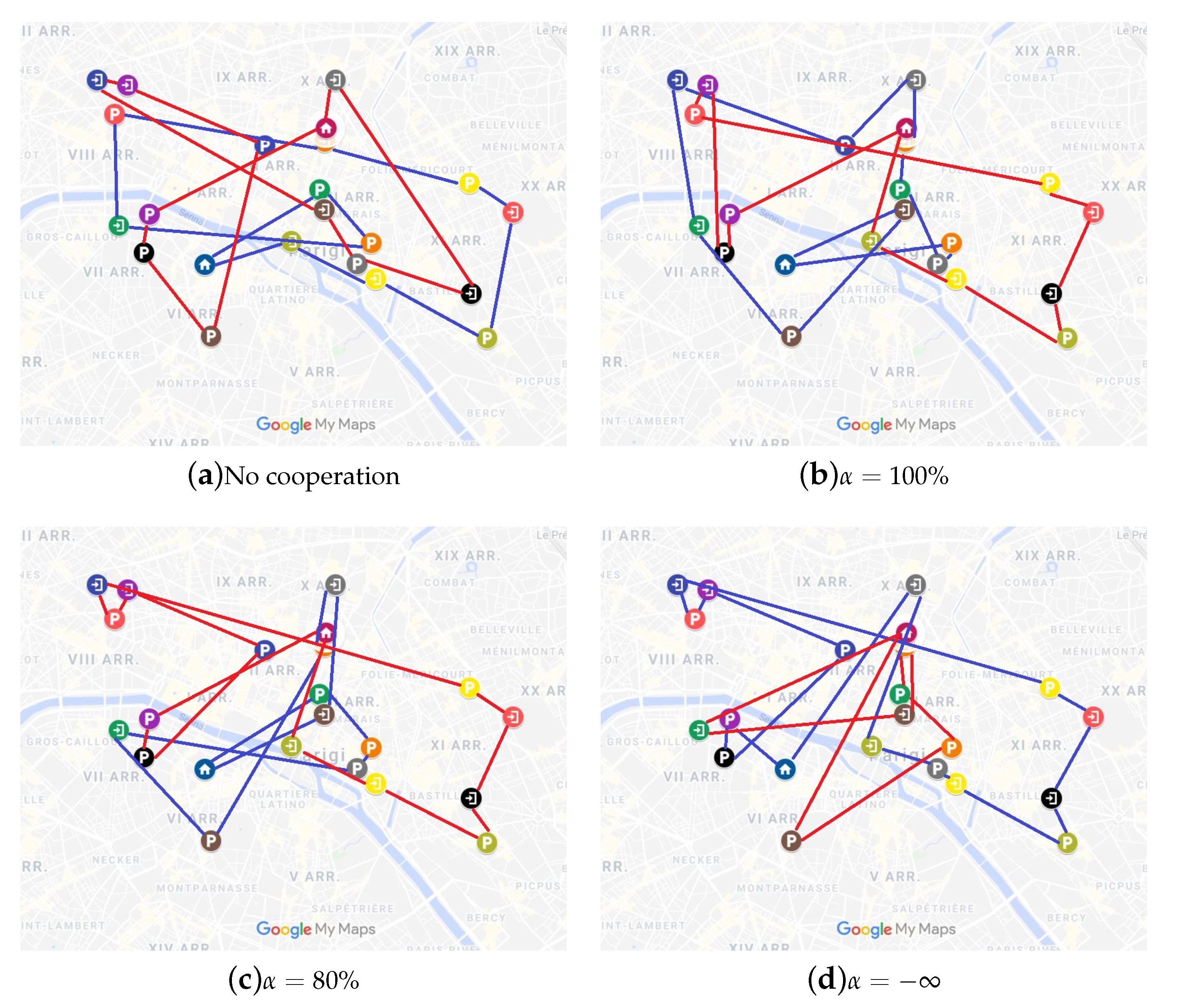
In Figure 1, the route plans of two different service providers (blue and red) obtained with different models and $\alpha$ values are represented. Figure 1a shows the usual noncooperative scheme in which each service provider serves its own customers realizing a total profit of 11,035, of which 5567 are related to the blue service provider and 5468 are related to the red service provider.

Conversely, Figure 1b represents the route plan obtained with the coop-SARP($\alpha$) model with $\alpha =100\%$, i.e., the model ensures that the profit of each service provider has to be at least the one they have in a noncooperative context. In this case, the total profit increases to 11,553 (+4.6%), with an individual increase for each service provider of +2.19% and +7.24%, respectively. Even if the number of customers served by each service provider remains stable, the growth of profits is possible thanks to the modified route plan, which allows them to save routing costs while maintaining balanced routes.

When $\alpha$ drops to 80%, as in Figure 1c, the resulting route plan is less balanced than the previous one. The model ensures that the profit of each service provider has to be at least 80% of the one they have in a noncooperative context, and hence, a service provider could earn less for the sake of improving the total profit. In this case, the total profit increases to 11,643 (+5.5%) with individual increases/decreases for each service provider equal to −12.95% and +24.31%, respectively. We note that, in this setting, a further improvement on the total profit could be obtained but some unfairness issues could be raised by service providers experiencing lower profits. This unfairness source is somewhat limited by the $\alpha$ value. Imbalances can be found also in the number of served customers, −20% and +20%, respectively.

Finally, unfairness could increase up to the extreme case where no thresholds on the losses are imposed, i.e., $\alpha =-\infty$, as shown in Figure 1d. In this case, the total profit increases to 11,793 (+6.87%) with individual increases/decreases for each service provider equal to +41.47% and −28.34%, respectively. These values would seriously affect the compliance of the service providers to the coalition, and the gain in terms of total profit with respect to a balanced route plan (as with $\alpha =100\%$) is less than humble. As a side effect, the imbalance in terms of served customers is even greater than the previous case.

The goal of the proposed formulation is to provide tools to foster cooperation among service providers while optimizing profits. This example suggests that a balanced approach to cooperation in terms of individual profits can be more satisfactory for agents and could increase the appeal of the system. At the same time, it could provide solutions with costs close to those obtained by full cooperation, i.e., $\alpha =-\infty$.

5. Computational Results

In this section, we provide a description of the instances (Section 5.1), the solution and model-based statistics (Section 5.2), and the results obtained (Section 5.3). All models and the procedure for the generation of the instances are implemented in Java v.8 and solved using CPLEX 12.6.0 on a Windows 64-bit computer with Intel Xeon processor E5-1650, 3.50 GHz, and 16 GB Ram. Before solving the models, the preprocessing techniques described in Cordeau [35] have been applied to speed up the computation.

5.1. Instance Generation

Because of the lack of benchmark instances for the cooperative SARP, we generate the following four groups of instances differing for the number of requests and service providers:

• Group A: eight requests equally distributed between two service providers
• Group B: ten requests equally distributed between two service providers
• Group C: six requests equally distributed between three service providers
• Group D: nine requests equally distributed between three service providers

Within each group, 40 instances are generated by choosing four different European metropolitan road networks: ten instances from Berlin, ten instances from Rome, ten instances from Paris, and ten instances from London. In total, we obtain 160 instances. Moreover, each instance is solved both in the noncooperative and cooperative settings. For the latter, three different values for $\alpha$ are considered, i.e., $\alpha =80\%$, $\alpha =90\%$, and $\alpha =100\%$ (we note that, beyond 100%, the solution may be infeasible because the service providers may not all simultaneously achieve a profit higher than the one in the noncooperative setting). Hence, each instance is considered under four different cooperative settings, leading to 640 instances in total.

Each request is represented by a couple of nodes (one for pickup and one for delivery). The nodes are taken from OpenStreetMap, and their features are extracted via Graphhopper. We first draw a rectangle corresponding to the city center ring, and then, the depot and the pickup and delivery address for each request are randomly chosen from the road network. Finally, the latitude and longitude for each node are returned together with the asymmetric distance matrix. In fact, the Graphhopper API allows us to extract the real distances also considering one-way streets, cars as means of transport, and minimum travel times as objectives for the shortest path from a point to another point. Moreover, each passenger request involves at most one person while each parcel request encompasses a volume that is uniformly randomly drawn from the interval $[0,Q_k^f]$. Time windows are created by solving a traveling salesman problem (with objective function 1 and with the aim of obtaining a feasible solution) on the customers of each service provider to determine the period at which the vehicle arrives at each customer. Then, to define the time window lower and upper bounds, we subtract and add 1000 s (around 16 min) to the desired visiting period, respectively, so that we obtained time windows of about half an hour.

Table 2. Parameter values shared across all instances.

Parameter		Value
$\mid {\mathcal{K}}_m\mid$		1
${\eta }_c$		$5*d_{ij}$
$\gamma$		$0.5$
${\rho }_c$		$5\%$${\eta }_c$
$s_i$		120 s
${\overline{r}}_c$		2000 s
$T_k$		20,000 s
$Q_k^p$		3
$Q_k^f$		300

displays the parameter values shared across all instances. Specifically, it contains the number of vehicles, the reward for each accepted request, the penalty for deviations of the passenger pickup from the time window, the penalty for not accepting a request, the service time at a node, the maximum ride time for each passenger, the maximum route duration, the maximum number of passengers, and the maximum number of parcels that can be carried simultaneously.

All instances can be found at https://valentinamorandi.it/research-outcomes/ (accessed on 9-04-2021).

5.2. Statistics

For each solution, we collected two categories of problem-based statistics, i.e., statistics for the whole system and statistics based on each service provider.

The statistics concerning the whole system are as follows:

• Objective function value, computed as $\Theta (\alpha )$.
• Profits, computed as rewards minus routing costs, i.e.,

  $$\sum _{k\in \mathcal{K}}\sum _{c\in \mathcal{C}}{\eta }_c{y}_c^k-\sum _{k\in \mathcal{K}}\sum _{i\in \mathcal{V}}\sum _{j\in \mathcal{V}}{d}_{ij}{x}_{ij}^k.$$
• Delay costs, i.e., ${\sum }_{k\in \mathcal{K}}{\sum }_{c\in {\mathcal{C}}^p}\gamma (l_{O_c}^k+l_{D_c}^k)$.
• Lost rewards, i.e., ${\sum }_{c\in \mathcal{C}}{\rho }_c(1-{\sum }_{k\in \mathcal{K}}{y}_c^k)$.

The statistics concerning the single service providers are as follows:

• Percentage of increase in served passenger requests with respect to the noncooperative setting, where the percentage of served passenger requests for a service provider is defined as ${\sum }_{c\in {\mathcal{C}}_m^p}{\sum }_{k\in {\mathcal{K}}_m}{y}_c^k/\mid {\mathcal{C}}_m^p\mid$.
• Percentage of increase in served parcel requests with respect to the noncooperative setting, where the percentage of served parcel requests by a service provider is defined as ${\sum }_{c\in {\mathcal{C}}_m^f}{\sum }_{k\in {\mathcal{K}}_m}{y}_c^k/\mid {\mathcal{C}}_m^f\mid$.
• Average occupancy rate of vehicles by passengers, computed as the time in which at least one passenger is carried over the total routing time, where the occupancy rate for each vehicle is computed as ${\sum }_{i\in \mathcal{V}}{\sum }_{j\in \mathcal{V}}{x}_{ij}^k{d}_{ij}{\omega }_i^k/{\sum }_{i\in \mathcal{V}}{\sum }_{j\in \mathcal{V}}{x}_{ij}^k{d}_{ij}$.
• Average occupancy rate of vehicles by parcels, computed as the time in which at least one parcel is carried over the total routing time, where the occupancy rate of each vehicle is computed as ${\sum }_{i\in \mathcal{V}}{\sum }_{j\in \mathcal{V}}{x}_{ij}^k{d}_{ij}{\lambda }_i^k/{\sum }_{i\in \mathcal{V}}{\sum }_{j\in \mathcal{V}}{x}_{ij}^k{d}_{ij}$.
• Average, minimum, and maximum increases in the profit of each service provider with respect to the noncooperative setting, where the profit is computed as the difference between rewards and routing cost, i.e.,

  $$\sum _{k\in {\mathcal{K}}_m}\sum _{c\in \mathcal{C}}{\eta }_c{y}_c^k-\sum _{k\in {\mathcal{K}}_m}\sum _{i\in \mathcal{V}}\sum _{j\in \mathcal{V}}{d}_{ij}{x}_{ij}^{k}m\in \mathcal{M}.$$
• Average, minimum, and maximum increases in travel times, where the travel time is computed as $u_{h_m^{{}^{\prime }}}^k-u_{h_m}^k$.

Finally, to analyze the dimension of the problem, we collected the following model-based statistics:

• Number of variables (continuous and integer)
• Number of constraints
• Runtime (in CPU seconds)

5.3. The Coop-SARP($\alpha$) Model against the Ncoop-SARP Model

In this section, we describe the results obtained by solving the coop-SARP($\alpha$) model for different values of $\alpha$ and we compare them to the noncooperative case, i.e., the Ncoop-SARP model (NC in tables and figures).

First, the behavior of the models in terms of CPU time and problem complexity is analyzed.

Table 3. Model-based statistics for instance groups A, B, C, and D and different levels of cooperation $\alpha$.

Group	Cooperation ($\mathit{\alpha }$)	Avg. CPU Time (s)	Avg. # Variables	Avg. # Constraints
A	NC	0.1	1040	2901.7
	100%	11.5	1040	2895.7
	90%	9.5	1040	2895.7
	80%	8.4	1040	2895.7
B	NC	0.5	1440	4064.7
	100%	2204.4	1440	4056.7
	90%	1193.0	1440	4056.7
	80%	274.2	1440	4056.7
C	NC	0.1	1296	3671.5
	100%	2.5	1296	3662.5
	90%	2.8	1296	3662.5
	80%	3.1	1296	3662.5
D	NC	0.4	2160	6214.5
	100%	969.5	2160	6199.5
	90%	725.6	2160	6199.5
	80%	1302.3	2160	6199.5

summarizes the model-driven statistics. From the third column of the table, we observe that the CPU runtime is highly affected by the number of requests in the considered instances. The highest CPU runtime is the one required for solving instances of group B (ten requests) and it is the lowest for instances of group C (six requests). By analyzing the CPU runtime for different levels of cooperation, the fastest case to solve is the noncooperative one because the decision about which service provider has to perform a service has not be made. For instances with a higher number of requests for each service provider (i.e., group A with four requests per service provider, and group B with five requests for service provider) and a cooperative setting, the closer the desired individual profit to the one of the noncooperative model, the higher the CPU runtime, despite the same number of variables and constraints. However, we cannot observe the same behavior for instances of groups C and D, where the number of service providers has been augmented but the number of requests per service provider has been lowered. Hence, there is no evidence of a direct connection between the level of cooperation and CPU time. To summarize, the results show that the complexity of the model increases due to the introduction of the cooperative setting in the model and by increasing the number of requests.

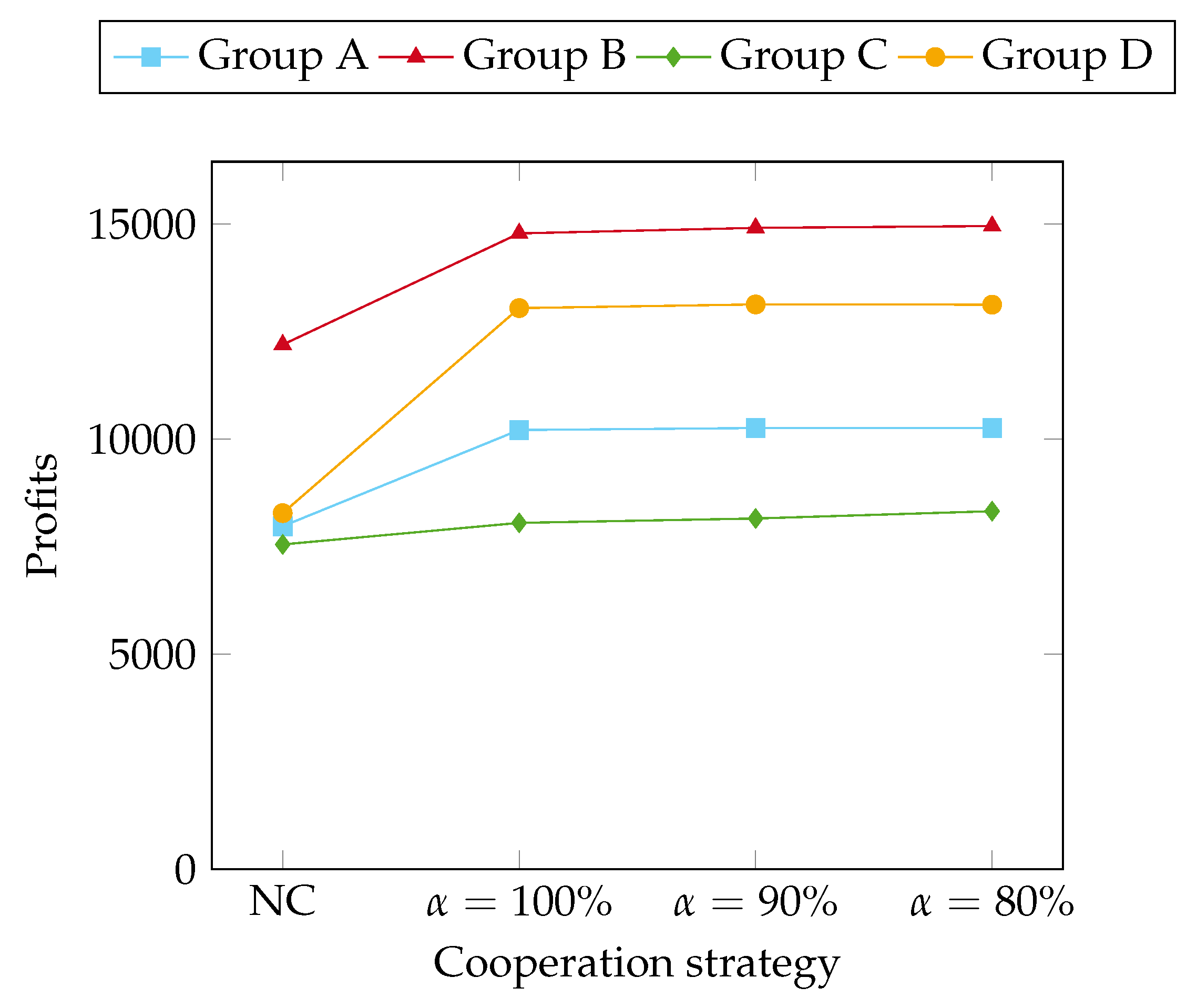
Second, we present the results concerning the statistics for the whole system. Figure 2 and Figure 3 represent the total objective function values and the profit (computed as the difference between the rewards and the routing costs) for the noncooperative setting and for the cooperative one with different levels of $\alpha$, respectively. In both figures, the objective function and the profit in cooperative settings are higher than the ones in the noncooperative model. Moreover, the lower $\alpha$, the higher the objective function and the profit. Recalling that lower levels of $\alpha$ stand for lower profit requirements from the individual service providers with respect to the profit they could achieve in noncooperative settings; this result suggests that the less pretentious service providers are, the higher the global benefit. Finally, the magnitude of the objective function and of the profits are proportional to the number of requests, i.e., higher for instance group B with ten requests and lower for instance group C with six requests.

Figure 4 represents the costs for delays in serving the passenger requests. By comparing the noncooperative and the cooperative results, the figure suggests that, except for instance group B, cooperation is not always beneficial for decreasing the costs for delays. Relating this result to Figure 2 and Figure 3, the motivation lies in the fact that, through cooperation, the reward for the additional served requests outweighs the small increase in delay costs significantly.

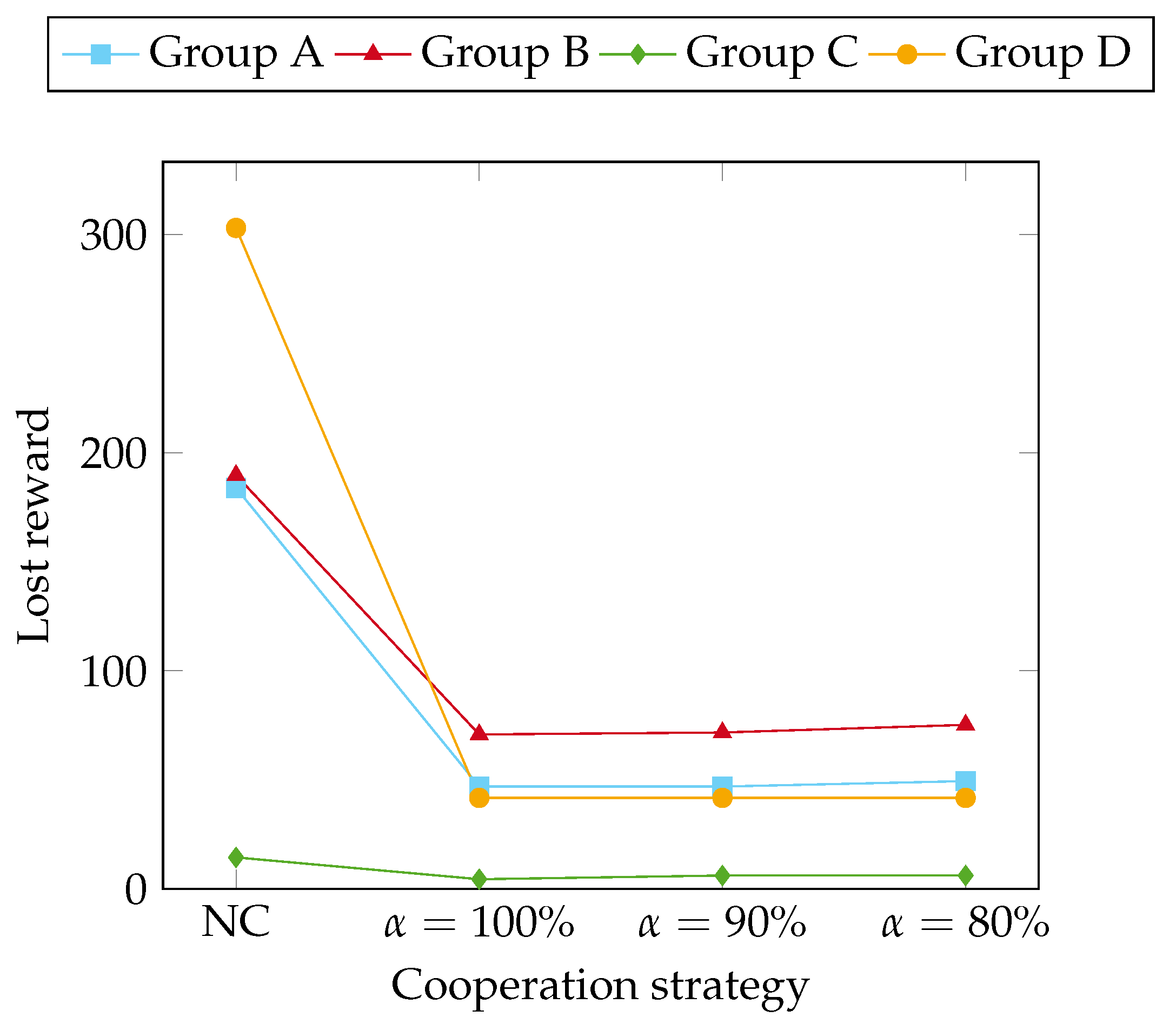
Figure 5 shows the lost reward across the different instance groups and for different cooperation levels. Once again, the benefits deriving from cooperation are outstanding, especially for instances with a high number of requests. However, the lost reward is stable for different levels of $\alpha$, suggesting that the requirement of a minimum level of profit in the cooperative case with respect to the noncooperative one does not play a crucial role in the amount of lost rewards.

Finally, having presented the metrics on how the model affects the whole coalition, statistics related to the impact on each service provider are analyzed.

Table 4. Increase in satisfied passengers and parcels with respect to the noncooperative case.

Group	Cooperation ($\mathit{\alpha }$)	Avg. Served Passengers (%)	Avg. Served Parcels (%)
A	100%	+35.4	+10.3
	90%	+35.4	+11.0
	80%	+31.1	+8.3
B	100%	+20.5	+5.9
	90%	+21.15	+4.1
	80%	+19.9	+4.1
C	100%	+1.8	+5.1
	90%	+1.8	+4.2
	80%	+1.8	+4.2
D	100%	+65.6	+13.2
	90%	+65.6	+13.8
	80%	+65.6	+13.8

presents the statistics associated with the service level in terms of increase in served requests with respect to the noncooperative case. Independently from the $\alpha$ parameter, the cooperative settings always allow for serving more passengers and parcels. The percentage of satisfied passengers and parcels dramatically increases implementing the coop-SARP($\alpha$) model, in most cases, more than 10%. The increase in the percentage of served passengers and parcels is lower for instance group C. This result is due to the presence of a few requests and a low number of requests per service provider, which allow the service providers to satisfy almost all requests also in the noncooperative setting. However, the contribution of the cooperation to the service level becomes more crucial as the number of requests per service provider decreases, as suggested by results on instances with a higher number of requests. The motivation relies on the fact that the lower the number of requests per service provider, the more flexible the system because it is easier to serve requests.

Table 5. Occupancy rate for passengers and parcels through the journeys.

Group	Cooperation ($\mathit{\alpha }$)	Occupancy Passengers (%)	Occupancy Parcels (%)
A	NC	35.5	56.2
	100%	48.2	62.3
	90%	47.9	63.3
	80%	48.1	60.7
B	NC	52.8	65.4
	100%	55.0	67.1
	90%	61.1	67.7
	80%	60.1	65.5
C	NC	29.2	34.8
	100%	36.1	36.1
	90%	35.4	35.5
	80%	36.9	36.1
D	NC	32.5	45.5
	100%	44.3	49.2
	90%	43.1	52.4
	80%	45.7	52.1

presents the statistics associated with vehicle occupancy both in terms of passengers and parcels with respect to the noncooperative case. Independently from the level of cooperation $\alpha$, the cooperative settings always accommodate passengers and parcels in such a way that the route plan is more efficient. In fact, the percentage of the routing time in which passengers and/or parcels are carried increases. The magnitude of the improvement in the occupancy rates depends on the instance size, but efficiency is always improved by at least 29.2% up to 67.7%. This result is explained by the higher number of served requests in the cooperative context and, hence, a better efficiency control with respect to the noncooperative setting.

Table 6. Maximum, minimum, and average increases in terms of profits among service providers.

Group	Cooperation ($\mathit{\alpha }$)	Max. Increase (%)	Min. Increase (%)	Avg. Increase (%)
A	100%	+24.3	+5.1	+14.7
	90%	+25.8	+2.8	+14.3
	80%	+28.8	+0.0	+ 14.4
B	100%	+41.5	+5.7	+23.6
	90%	+45.8	+1.5	+23.6
	80%	+48.9	+0.1	+24.5
C	100%	+32.4	+1.5	+12.7
	90%	+40.8	−1.6	+14.7
	80%	+52.1	−5.1	+17.5
D	100%	+76.1	+0.8	+32.1
	90%	+81.8	−0.8	+32.7
	80%	+83.7	−2.7	+ 32.7

shows the distribution of the growth of profits among service providers joining the coalition with respect to the noncooperative case. Here, the $\alpha$ parameter shows its crucial role. Using $\alpha$ values lower than 100% allows the model to realize negative profits for a few unlucky service providers. Although this phenomenon could surely happen (see instances C and D for $\alpha =80,90\%$), the minimum increase is always negligible with respect to the maximum increase, which is always far superior. In addition, the average value is always very high, suggesting a general trend where the model rewards all service providers. Obviously, unfairness increases with lower values of $\alpha$. For this reason, the coalition should agree in advance with the $\alpha$ level that is acceptable for all service providers. In fact, as shown in the detailed example in Section 4, without imposing constraints on the realized profit, severe unfairness issues arise.

Finally, in

Table 7. Increase in travel time with respect to Ncoop-SARP among all service providers (max, min, and avg).

Group	Cooperation ($\mathit{\alpha }$)	Max. (%)	Min. (%)	Avg. (%)
A	100%	+16.0	−12.3	+1.8
	90%	+16.8	−14.6	+1.1
	80%	+17.2	−16.2	+0.5
B	100%	+7.0	−17.2	−5.1
	90%	+4.2	−19.9	−7.9
	80%	+5.8	−20.9	−7.5
C	100%	+6.7	−14.6	−3.9
	90%	+10.6	−23.1	−6.5
	80%	+14.9	−34.5	−8.9
D	100%	+15.0	−23.7	−4.4
	90%	+15.1	−25.9	−5.5
	80%	+16.6	−27.5	−5.2

, the increase in terms of workload, i.e., travel time, with respect to the noncooperative case is shown. For profits, the table shows the best (Min (%)), the worst (Max (%)), and the average case (Avg. (%) to let the reader understand the distribution of the increase in workload. Although the workload globally increases because more requests are served, for instances, in groups B, C, and D, the average workload decreases and, in group A, it only slightly increases, the minimum workload increase is always significantly low and, in most cases, it effectively counterbalances the maximum increase.

6. Conclusions

In this paper, we proposed a novel mathematical programming formulation, i.e., the coop-SARP, which, starting from an extension of the classical SARP, includes more realistic features of the problem as the presence of multiple service providers (each one with its own depot and a different vehicle fleet) and the presence of horizontal cooperation among them. The proposed formulation is capable of considering different levels of cooperation, and theoretical results on the lower and upper bounds have been derived. Due to the lack of benchmark instances in the literature for this problem and to let computational results represent real-world cases, we generated map-based instances from four European metropolitan road networks. Through numerical experiments and ad hoc devised statistics, we analyzed the benefits of different levels of horizontal cooperation in SARP models. The results show that all agents in the system benefit from horizontal cooperation. First, travel times decrease considerably and the occupancy rates of vehicles improve. This is an important finding for a city logistic context in which congestion reduction is one of the priorities. Second, the number of satisfied requests increases with respect to a noncooperative setting. This leads to an improved service level, from which customers can benefit. Finally, we showed how an agreed balanced approach to cooperation may yield more satisfactory profits for service providers and, hence, increase the appeal of the system.

Multiple future developments could arise starting from this study on cooperation in SARP models. Additional problem characteristics could be considered, such as multi-modal trips or the possibility of transferring passengers and parcels between vehicles. Moreover, our model-based statistics show that small instances for this problem are already challenging to be solved by an off-the-shelf solver in reasonable runtimes. For this reason, an interesting research direction could consist in the development of metaheuristics for this problem to address larger and more realistic instances. Finally, a new set of benchmark instances for the coop-SARP could be proposed by extending the instances available in the literature for the SARP and for the DARP.

References

- Savelsbergh, M.; Van Woensel, T. 50th anniversary invited article—City logistics: Challenges and opportunities. Transp. Sci. 2016, 50, 579–590. [Google Scholar] [CrossRef]
- Mangano, G.; Zenezini, G.; Cagliano, A.C. Value Proposition for Sustainable Last-Mile Delivery. A Retailer Perspective. Sustainability 2021, 13, 3774. [Google Scholar] [CrossRef]
- Demir, E.; Huang, Y.; Scholts, S.; Van Woensel, T. A selected review on the negative externalities of the freight transportation: Modeling and pricing. Transp. Res. Part Logist. Transp. Rev. 2015, 77, 95–114. [Google Scholar] [CrossRef]
- Macioszek, E. First and last mile delivery—Problems and issues. In Scientific And Technical Conference Transport Systems Theory And Practice; Springer: Cham, Switzerland, 2017; pp. 147–154. [Google Scholar]
- NHT Survey. Summary of Travel Trends; Federal Highway Administration Office of Policy and Governmental Affairs, USA. 2017. Available online: https://www.fhwa.dot.gov/policyinformation/documents/2017_nhts_summary_travel_trends.pdf (accessed on 9 April 2021).
- Guerlain, C.; Renault, S.; Ferrero, F.; Faye, S. Decision support systems for smarter and sustainable logistics of construction sites. Sustainability 2019, 11, 2762. [Google Scholar] [CrossRef] [Green Version]
- Macioszek, E. Freight transport planners as information elements in the last mile logistics. In Scientific and Technical Conference Transport Systems Theory And Practice; Springer: Cham, Switzerland, 2018; pp. 242–251. [Google Scholar]
- Stiglic, M.; Agatz, N.; Savelsbergh, M.; Gradisar, M. The benefits of meeting points in ride-sharing systems. Transp. Res. Part Methodol. 2015, 82, 36–53. [Google Scholar] [CrossRef] [Green Version]
- Levin, Y.; Nediak, M.; Topaloglu, H. Cargo capacity management with allotments and spot market demand. Oper. Res. 2012, 60, 351–365. [Google Scholar] [CrossRef]
- Lindholm, M.; Behrends, S. Challenges in urban freight transport planning—A review in the Baltic Sea Region. J. Transp. Geogr. 2012, 22, 129–136. [Google Scholar] [CrossRef]
- Cleophas, C.; Cottrill, C.; Ehmke, J.F.; Tierney, K. Collaborative urban transportation: Recent advances in theory and practice. Eur. J. Oper. Res. 2019, 273, 801–816. [Google Scholar] [CrossRef]
- Mourad, A.; Puchinger, J.; Chu, C. A survey of models and algorithms for optimizing shared mobility. Transp. Res. Part Methodol. 2019, 123, 323–346. [Google Scholar] [CrossRef]
- Li, B.; Krushinsky, D.; Reijers, H.A.; Van Woensel, T. The share-a-ride problem: People and parcels sharing taxis. Eur. J. Oper. Res. 2014, 238, 31–40. [Google Scholar] [CrossRef]
- Molenbruch, Y.; Braekers, K.; Caris, A. Benefits of horizontal cooperation in dial-a-ride services. Transp. Res. Part Logist. Transp. Rev. 2017, 107, 97–119. [Google Scholar] [CrossRef]
- Li, B.; Krushinsky, D.; Van Woensel, T.; Reijers, H.A. The Share-a-Ride problem with stochastic travel times and stochastic delivery locations. Transp. Res. Part Emerg. Technol. 2016, 67, 95–108. [Google Scholar] [CrossRef]
- Beirigo, B.A.; Schulte, F.; Negenborn, R.R. Integrating people and freight transportation using shared autonomous vehicles with compartments. IFAC-PapersOnLine 2018, 51, 392–397. [Google Scholar] [CrossRef]
- Cordeau, J.F.; Laporte, G. The dial-a-ride problem: Models and algorithms. Ann. Oper. Res. 2007, 153, 29–46. [Google Scholar] [CrossRef]
- Qu, Y.; Bard, J.F. The heterogeneous pickup and delivery problem with configurable vehicle capacity. Transp. Res. Part Emerg. Technol. 2013, 32, 1–20. [Google Scholar] [CrossRef]
- Häll, C.H.; Andersson, H.; Lundgren, J.T.; Värbrand, P. The integrated dial-a-ride problem. Public Transp. 2009, 1, 39–54. [Google Scholar] [CrossRef] [Green Version]
- Masson, R.; Lehuédé, F.; Péton, O. The dial-a-ride problem with transfers. Comput. Oper. Res. 2014, 41, 12–23. [Google Scholar] [CrossRef]
- Paquette, J.; Cordeau, J.F.; Laporte, G.; Pascoal, M.M. Combining multicriteria analysis and tabu search for dial-a-ride problems. Transp. Res. Part Methodol. 2013, 52, 1–16. [Google Scholar] [CrossRef] [Green Version]
- Lehuédé, F.; Masson, R.; Parragh, S.N.; Péton, O.; Tricoire, F. A multi-criteria large neighbourhood search for the transportation of disabled people. J. Oper. Res. Soc. 2014, 65, 983–1000. [Google Scholar] [CrossRef]
- Reinhardt, L.B.; Clausen, T.; Pisinger, D. Synchronized dial-a-ride transportation of disabled passengers at airports. Eur. J. Oper. Res. 2013, 225, 106–117. [Google Scholar] [CrossRef]
- Hanne, T.; Melo, T.; Nickel, S. Bringing robustness to patient flow management through optimized patient transports in hospitals. Interfaces 2009, 39, 241–255. [Google Scholar] [CrossRef]
- Beaudry, A.; Laporte, G.; Melo, T.; Nickel, S. Dynamic transportation of patients in hospitals. OR Spectr. 2010, 32, 77–107. [Google Scholar] [CrossRef] [Green Version]
- Parragh, S.N.; Cordeau, J.F.; Doerner, K.F.; Hartl, R.F. Models and algorithms for the heterogeneous dial-a-ride problem with driver-related constraints. OR Spectr. 2012, 34, 593–633. [Google Scholar] [CrossRef] [Green Version]
- Schilde, M.; Doerner, K.F.; Hartl, R.F. Metaheuristics for the dynamic stochastic dial-a-ride problem with expected return transports. Comput. Oper. Res. 2011, 38, 1719–1730. [Google Scholar] [CrossRef] [Green Version]
- Detti, P.; Papalini, F.; de Lara, G.Z.M. A multi-depot dial-a-ride problem with heterogeneous vehicles and compatibility constraints in healthcare. Omega 2017, 70, 1–14. [Google Scholar] [CrossRef]
- Molenbruch, Y.; Braekers, K.; Caris, A. Typology and literature review for dial-a-ride problems. Ann. Oper. Res. 2017, 259, 295–325. [Google Scholar] [CrossRef]
- Parragh, S.N.; Pinho de Sousa, J.; Almada-Lobo, B. The dial-a-ride problem with split requests and profits. Transp. Sci. 2014, 49, 311–334. [Google Scholar] [CrossRef]
- Garaix, T.; Artigues, C.; Feillet, D.; Josselin, D. Optimization of occupancy rate in dial-a-ride problems via linear fractional column generation. Comput. Oper. Res. 2011, 38, 1435–1442. [Google Scholar] [CrossRef] [Green Version]
- Posada, M.; Andersson, H.; Häll, C.H. The integrated dial-a-ride problem with timetabled fixed route service. Public Transp. 2017, 9, 217–241. [Google Scholar] [CrossRef] [Green Version]
- Toth, P.; Vigo, D. Vehicle Routing: Problems, Methods, and Applications; SIAM: Philadelphia, PA, USA, 2014. [Google Scholar]
- Ho, S.C.; Szeto, W.; Kuo, Y.H.; Leung, J.M.; Petering, M.; Tou, T.W. A survey of dial-a-ride problems: Literature review and recent developments. Transp. Res. Part Methodol. 2018, 111, 395–421. [Google Scholar] [CrossRef]
- Cordeau, J.F. A branch-and-cut algorithm for the dial-a-ride problem. Oper. Res. 2006, 54, 573–586. [Google Scholar] [CrossRef] [Green Version]
- Ropke, S.; Cordeau, J.F.; Laporte, G. Models and branch-and-cut algorithms for pickup and delivery problems with time windows. Networks 2007, 49, 258–272. [Google Scholar] [CrossRef]
- Braekers, K.; Kovacs, A.A. A multi-period dial-a-ride problem with driver consistency. Transp. Res. Part Methodol. 2016, 94, 355–377. [Google Scholar] [CrossRef] [Green Version]
- Feng, L.; Miller-Hooks, E.; Schonfeld, P.; Mohebbi, M. Optimizing ridesharing services for airport access. Transp. Res. Rec. 2014, 2467, 157–167. [Google Scholar] [CrossRef]
- Gschwind, T.; Irnich, S. Effective handling of dynamic time windows and its application to solving the dial-a-ride problem. Transp. Sci. 2014, 49, 335–354. [Google Scholar] [CrossRef]
- Desrochers, M.; Lenstra, J.K.; Savelsbergh, M.W.; Soumis, F. Vehicle Routing with Time Windows: Optimization and Approximation; Technical Report; CWI, Department of Operations Research and System Theory [BS]: Amsterdam, The Netherlands, 1987. [Google Scholar]
- Desrosiers, J.; Dumas, Y.; Solomon, M.M.; Soumis, F. Time constrained routing and scheduling. Handb. Oper. Res. Manag. Sci. 1995, 8, 35–139. [Google Scholar]
- Desrochers, M.; Laporte, G. Improvements and extensions to the Miller-Tucker-Zemlin subtour elimination constraints. Oper. Res. Lett. 1991, 10, 27–36. [Google Scholar] [CrossRef]
Figure 1.
Service assignment to service providers under different operating scenarios (pickup ![Sustainability 13 04362 i001]() , delivery points
, delivery points ![Sustainability 13 04362 i002]() , and depots
, and depots ![Sustainability 13 04362 i003]() ). For the sake of representation clarity, the connections between nodes are represented by segments, but in this work, map-based connections and distances have been considered.
). For the sake of representation clarity, the connections between nodes are represented by segments, but in this work, map-based connections and distances have been considered.
, delivery points
, and depots
, delivery points , and depots ). For the sake of representation clarity, the connections between nodes are represented by segments, but in this work, map-based connections and distances have been considered.
Figure 2.
Objective function values for instance groups A, B, C, and D and different cooperation levels.
Figure 3.
Profits (rewards minus routing costs) for instance groups A, B, C, and D and different cooperation levels.
Figure 4.
Delay costs for instance groups A, B, C, and D and different cooperation levels.
Figure 5.
Lost reward for instance groups A, B, C, and D and different cooperation levels.