
Dynamic Electricity Intensity Trends in 91 Countries

1
Department of Global Business, Gachon University, 1342 Seongnam-daero, Sujung-gu, Gyeonggi-do 13120, Korea
2
Gachon Center for Convergence Research, Gachon University, 1342 Seongnam-daero, Sujung-gu, Gyeonggi-do 13120, Korea
*
Author to whom correspondence should be addressed.
Sustainability 2021, 13(8), 4588; https://0-doi-org.brum.beds.ac.uk/10.3390/su13084588
Submission received: 19 November 2020
/
Revised: 12 April 2021
/
Accepted: 16 April 2021
/
Published: 20 April 2021
(This article belongs to the Section Energy Sustainability)
Abstract
:Despite numerous studies on energy productivity and efficiency, only a few focus on the electricity intensity (EI) of economic output. As these studies largely examine the declining trend in EI, the increasing and/or fluctuating trends in EI have not been studied. We analyze EI trends by estimating the progress ratios from experience curves of 91 countries from 1991 to 2011. The results reveal wide variation in progress ratios, ranging from 53% to 135%, with an average of 101.5%. Furthermore, more than half of the 91 countries displayed a kinked slope, indicating the fluctuating rate of change in EI. The rate of population growth seems to be related to the increasing EI trends. A clear understanding of the relative performance of each country in terms of the progress ratio and the pattern of EI trends would be useful for the country’s policymakers to develop strategic options for the future.
1. Introduction
Electricity is one of the most dominant forms of energy in human society. Its flexibility, reliability, and efficiency as an energy carrier have led to an increase in its share in total energy consumption in almost all countries worldwide. Electricity accounted for 19.3% of global final energy needs in 2018, up from 9.4% in 1973 [1]. The share of global primary energy used to generate electricity has steadily increased from 11.2% in 1980 to 25.7% in 2018 [2]. Among all the final energy carriers, electricity has exhibited the highest per capita consumption growth, from 1347 kWh per capita in 1974 to 2163 kWh per capita in 1994 and further to 3132 kWh per capita in 2014 [3]. The International Energy Agency (IEA) expects the global demand for electricity to grow twice as fast as that for primary energy and forecasts the share of electricity to increase from 19% in 2018 to 24% in 2040. In the IEA’s Sustainable Development Scenario, electricity is expected to account for an even higher share of final energy consumption [4].
Electricity is especially important because it is closely related to economic growth. One measure of how electricity is related to economic growth is electricity intensity (EI), represented as the ratio of the amount of electricity generated to the gross domestic product (GDP) of a country. According to the International Energy Outlook (IEO) 2016, the world’s net electricity generation (NEG) in 2012 was 21,600 billion kWh compared to the world GDP of USD 94,455 billion (in 2010 U.S. dollars, adjusting for purchasing power parity) [5]. Therefore, the 2012 EI was 0.23 KWh per dollar. It also projects an NEG of 36,500 billion kWh and a GDP of USD 236,831 billion in 2040, implying a decrease in EI to 0.15 KWh per dollar. This is because the world’s GDP is projected to grow at 3.3% per year, which is faster than NEG at 1.9% per year. As the biggest source of greenhouse gas emissions, electricity and its efficient use are of great interest to environmental policy designers [6]. For example, in the United Nation’s Sustainable Development Goals, Goal 13 on climate change is directly related to greenhouse gas emissions, and Goal 7 on energy and 11 on urbanization are also relevant [7].
We analyze EI trends in 91 countries from 1991 to 2011 by estimating progress ratios (PRs) from experience curves (ECs). Although EI has recently begun to attract more attention in the literature, previous studies focused either on the factors affecting EI in a single or a small number of countries [8,9,10] or its convergence across countries [11,12,13]. We attempt to contribute to the literature on EI by analyzing the EI trends in 91 countries over two decades. The benefit of using EC is that the change in EI trends for individual countries can be identified, thereby enabling more detailed policy suggestions. Additionally, an EC analysis allows us to identify whether and when a dramatic change in the EI trend occurs. We identify four different types of ECs—increasing classical, increasing kinked, decreasing classical, and decreasing kinked—and suggest various possibilities for improving EIs in the future depending on the types of ECs.
The rest of this paper is organized into the following sections. Section 2 briefly reviews the previous studies on EI. Section 3 reviews the application of EC to energy research. Section 4 explains the data and method used. Section 5 presents the results of the analysis and those of the robustness test, which extends the research period to 2018 for the five largest electricity producing countries. Finally, the conclusion and limitations of our findings are presented in Section 6.
2. Previous Research on EI
Although several studies have analyzed energy intensity trends and the reasons thereof, EI has received little attention [11]. Previous studies on EI can be classified into two groups: one comparing and analyzing the change in EI across countries and/or over time and the other investigating the factors affecting EI (Table 1).
2.1. Research on the Comparison and Convergence of EI
The comparison of EI changes over time across countries has received relatively limited attention. In a comparative study of 24 Organization for Economic Co-operation and Development (OECD) countries and South Africa, Inglesi-Lots and Blignaut [13] reported a wide variation in EIs. In 2007, for example, Iceland recorded the highest and Ireland the lowest EI of 1.27 and 0.18, respectively. The countries in the study displayed a wide variation, even in terms of long-term (from 1990 to 2007) change in EI while Norway, Sweden, and Canada recorded changes in EI of −32%, −30%, and −24%, respectively; Poland, Hungary, Mexico, and Turkey were on the other side of the continuum with an EI increase of 382%, 401%, 493%, and 1200%, respectively. Comparing EIs among 22 Asia-Pacific economies from 1994 to 2014, Hien [14] also documented a variance in the EI trends in two groups of countries: a moderate increase in EIs for most developing countries and a decrease for developed economies. A wide variation was again reported, ranging from an increase of 400% for Vietnam to a decrease of 41% for Mongolia during the 1985–2014 period.
Other studies investigated the issue of convergence, that is, whether the difference in EIs across (groups of) countries diminishes over time. Liddle [15] illustrated that the overall variance in EI among 22 OECD countries decreased from 1960 to 2005 because the countries with high EIs, such as Norway, Sweden, and Finland, experienced a downward trend, whereas many other countries exhibited an increasing trend. However, different convergence patterns were reported depending on end-use sectors: whereas commercial EIs converged toward a bell-shape distribution, industrial EIs converged toward a bimodal distribution. More recently, Kim [12] examined EI convergence between 1971 and 2009 using data from 109 countries and reported that EI converged for all countries but the per capita electricity consumption converged only for developed countries. These two studies present strong evidence that the difference in EIs across countries has diminished over four decades.
China provides an interesting research context to study the issue of EI convergence for many reasons, including the rapid economic growth and the provincial differences generating within-country diversity. Using the provincial panel data in China, Herrerias and Liu [8] found evidence for EI convergence as a country, suggesting that technological differences across provinces diminished from 2003 to 2009. However, the convergence existed within groups of regions and some regions still diverged. Further, seasonal fluctuations between increasing and decreasing trends occurred for the country as a whole, as well as for several provinces [9].
2.2. Research on the Determinants of EI
A few studies analyzed the relative contribution of structural change and intensity effects to EI. Using data for Spain from 1979 to 1992, Fernández and Pérez [16] demonstrated that structural effects, that is, changes in the sectoral mix of the economy, were a poor contributor to EI decline, whereas intensity effects, such as technological progress and productivity increase, were dominant contributors. Vaona [17], in the study of Italian regions, also illustrated the role of intensity effects on EI trends and argued that the industry mix played a minor role with the intensity effects held constant. However, Wenzel and Wolf [18] found that the contribution of structural effects to EI decline varied across countries. For example, restructuring to less electricity-intensive manufacturing played an important role in decreasing EI only in the case of Hungary, Poland, and the Czech Republic. However, unlike structural effects, intensity effects consistently contributed to EI reduction in all countries in the sample, except Bulgaria.
Several studies employed econometric analyses to identify factors affecting EI. Kwon et al. [10] examined the effects of electricity price on EIs in the manufacturing sector across 16 regions in South Korea. Using 108 months of panel data, they found evidence that increases in electricity price decreased EIs only in the long run, and the effects varied over time and regions. This is consistent with the finding by Verbruggen [19] that high end-use electricity prices are a precondition for low EIs. Recently, Gutiérrez-Pedrero et al. [11] investigated the factors influencing EIs in the non-residential sectors of 13 European Union countries. The results demonstrated that technological progress and increases in the electricity price decreased EIs, whereas the stock of physical capital and investment increased EIs.
Besides economic factors, government initiatives to raise awareness of the importance of EI among the public have been highlighted in a couple of studies. Employing a fixed-effects panel model, Horowitz [20] analyzed commercial sector EIs across 24 states in the U.S. from 1989 to 2001. The results illustrate that, controlling for market factors, public programs on demand side management led to a decrease in EIs. Ullah et al. [21] reported a similar finding in a developing-country context by analyzing EIs in Pakistan from 1972 to 2012 and revealed that education was a significant factor in reducing the country’s EI by increasing the awareness of the potential crisis because of electricity shortage. They also demonstrated that the increase in per capita income led to EI deterioration, while the impact of price change on EI was limited.
The literature survey on EI trends identified two major research gaps for us to examine. First, how significant is the number of countries experiencing an increasing EI trend compared to a decreasing EI trend, during a study period? Second, how many countries have experienced fluctuating rates of change in EI during a study period? As these two questions have not been systematically analyzed for multiple countries, we include all countries with matching data available for the period from 1991 to 2011. Further, we use two types of ECs, classical and kinked, instead of the simple average annual rate of change to estimate the rate of change in EIs. The PR estimated from the EC represents the rate of change in EI as a function of doubling cumulative NEG for individual countries. The use of a kinked EC also enables us to estimate multiple rates of change during the study period. The PRs for all 91 countries are estimated and ranked in ascending order. We then estimate the average PR, standard deviation (SD), and coefficient of variation (CV) for the total sample, as well as for subgroups of countries, categorized by the type of PR (increasing versus decreasing, single versus multiple), income, and region.
Our analysis distinguishes between countries that have reduced their EIs (i.e., better-performing countries) and those that have increased their EIs. We then list the countries that are likely to sustain their decreasing EI trends in the future. The results also suggest which countries are more likely to reduce their future EIs by reversing their past increasing EI trends. To the best of our knowledge, the abovementioned research questions have never been examined using the EC to estimate the PRs of EIs for as many as 91 countries. Thus, this study may provide new insights into the EI research literature.
3. Brief Review of EC
The accumulation of experience has been observed to increases productivity in many industries by lowering the inputs required to make a unit of a product. For instance, Wright [22] found that the average person-hours required to assemble a Boeing aircraft decreased by 20% as the cumulative number of airplanes assembled doubled. This effect is referred to as the learning curve and reflects the philosophy of learning by doing. Applying this philosophy to the relationship between total costs and outputs, the Boston Consulting Group (BCG) [23] introduced the EC model. They investigated the reduction rate of unit costs in constant dollars with every increase in the cumulative volume of production for 24 products. The result illustrated that the ratio of the final to the initial costs incurred in doubling the cumulative volume, which was termed as the PR, was 70% to 80%. However, BCG made an important modification to the original learning curve model, allowing it to capture total cost elements such as R&D, sales expenses, advertising, overhead, and intangibles, which are required to deliver the product to ultimate users. Given that BCG expanded the concept of input from a single variable to include the total cost elements, EC became a widely used tool to analyze the learning effect at not only the factor level but also at the firm and industry levels.
One area where the learning effect has a significant influence is energy technology. With increasing concerns about the impact of greenhouse gas emissions and oil-derived fuels on the climate, building and maintaining sustainable energy systems has received significant attention. To reflect the long-term experience effect, researchers and practitioners have extensively applied the EC approach in their analysis. For instance, the average PR computed from various studies on energy supply technology [24,25,26] is 84%. Applying the model to different energy demand technologies, including automobiles and home electronics, Weiss et al. [27] found PRs ranging from 59% to 96%.
Several scholars have been attempted to extend the EC analysis. First, recent studies considered not only the simple learning effect but also other sources of experiences as independent variables. These include learning by consuming [28], learning by knowledge spillover [29], and learning by learning [30]. Further, more recent studies argue that the observed improvement effects are the outcome of the accumulation of multiple learning processes beyond single inputs [31]. Second, the EC approach has also adopted several physical performance measures such as energy or carbon intensity. For example, the EC approach was employed by Nakicenovic [32] to analyze the historical trend in carbon intensity in the U.S., and by IEA [33] to assess energy intensities in global markets.
ECs are capable of analyzing not only a decreasing but also an increasing trend in a performance metric. For example, Grubler [34] used ECs to estimate the positive experience slope for increasing reactor construction costs per kilowatt-hour of nuclear power as a function of cumulative installed capacity in both France and the U.S. A positive experience slope translates into a PR value exceeding 100%. Similarly, positive experience slopes have been reported for natural gas-fired power plants [35] as well as on-shore wind power [36]. Learning rates are typically not the same throughout the lifecycle of a technology [37]. Sometimes, such changes in the slope are caused by technological breakthroughs [38]. In other cases, experience slopes become steeper in the later development stages of several renewable energy technologies [39]. Under these circumstances, traditional ECs can be modified to accommodate multiple experience slopes over a lifecycle. Such modified ECs with a kink (piecewise linear) in the slope, known as kinked ECs, have been used in several studies [40,41,42,43]. In summary, ECs can deal with both increasing and decreasing trends in performance outcomes of variables, such as EI, and can also estimate multiple rates of change over a lifecycle. Compared to the use of time as an independent variable, ECs are a more flexible method of estimating the rate of change in EI.
4. Data and Method
We define historical yearly EI (EIt) as follows:
where t runs from 1991 through 2011.
NEG in time t (NEGt), measured in billion kWh, is obtained from the EIA’s webpage on international energy statistics [44]. GDP in time t (GDPt), based on 2011 constant U.S. billion dollars adjusted by the purchasing power parity, is sourced from the World Bank [45]. We then divide NEGt by GDPt to obtain EI for each year. To get an understanding of what happened in terms of EI, we present the historical pattern of EIs from 1991 to 2011 in Figure 1 for the five largest producers of electricity in the world: China, the U.S., Japan, India, and Canada. The U.S. and Canada display a more rapidly declining trend, whereas China and India show a moderately decreasing trend. Japan is the only country with a moderately increasing trend.
Two types of ECs, namely classical and kinked, are specified as follows [40]. In both ECs, the dependent variable for a country is the EI and the independent variable is the cumulative NEG from 1991 to year t.
The classical EC equation for each country is defined as follows:
where t = 1991, 1992, …, 2011,
y(xt) = axtb
y(xt) = EI in year t,
xt = the cumulative NEG from year 1991 to year 2011,
a = constant, and
b = experience slope.
In logarithmic form, the classical experience equation is expressed as follows:
lny(xt) = lna + blnxt.
The kinked experience equations of EI for an individual country are defined if a break point occurs at the year k as
where a1 and b1 are parameters for Equation (4) from year 1991 to year k − 1, and
where a2 and b2 are parameters for Equation (5) from year k to year 2011.
y(xt) = a1xtb1,
y(xt) = a2xtb2
In logarithmic form, the kinked experience equation for the first period (Equation (4)) would be
and the kinked experience equation for the second period (Equation (8)) would be
lny(xt) = lna1 + b1lnxt
lny(xt) = lna2 + b2lnxt
We can combine the two logarithmic form kinked experience equations using a dummy variable that takes the value of one if the year belongs to the second period and zero otherwise:
where p = 0 if t = 1991, 1992, …, k − 1, and p = 1 if t = k, k + 1, …, 2011.
lny(xt) = lna1 + (lna2 − lna1) × p + b1lnxt + (b2 − b1)lnxt × p
In the kinked experience model, k is the year when a kink in the pattern of EI occurs. Parameters are estimated by running an OLS regression, which was adopted by many EC studies as an empirical model [33,46,47,48]. EC studies rely on, by definition, time series data, which typically show an upward or a downward trend. Even though the nature of time series data raises a methodological issue, EC as a forecast model has been shown to work reasonably well [49]. Alberth [46] conducted a forecast assessment by dividing the dataset into two, one of which was used to forecast and the other to compare forecasts with the actual realized value, and found the difference between the two statistically insignificant. Using the systematic hindcasting method, Nagy et al. [48] and Farmer and Lafond [50] reported that EC made reasonably good forecasts. Neij [51] also showed that the results of the EC studies were similar to those of the bottom-up analysis, in most cases.
We consider all the possible years for the kinked year and compute the R2 or the coefficient of determination, which denotes the goodness of fit of an equation. We then choose the year with the largest R2 as the kinked year. Thus, the kinked year may vary by country.
Next, for Equation (8) with the largest R2, we test whether or not the difference between b1 and b2 is statistically significant—if not, we can conclude that the relationship between the EI and the NEG does not differ between the first and second periods. Thus, the classical EC model should be used for this case. However, if the difference between b1 and b2 is statistically significant, we can conclude that the relationship between the EI and NEG differs between the first and second periods. Thus, the kinked EC model should be used for this case. In particular, the relationship between the EI and NEG for the second period is used.
The PR for the cumulative doubling of NEG is computed by the equation PR = 2b and the learning rate (LR) is defined as LR = 1 − PR [39], that is, PR represents the rate of change in EI as a doubling function of cumulative NEG. For example, if PR is 80%, then each doubling of cumulative NEG will require 20% less EI; if PR is 120%, then each doubling of cumulative NEG will require 20% more EI. In other words, if EI shows a decreasing historical trend, PR would be less than 100%. Under these circumstances, doubling the cumulative NEG will require a proportionately lower EI, indicating higher electricity productivity. Conversely, if EI shows an increasing historical trend, PR would be greater than 100%, and doubling the cumulative NEG will require a proportionately greater EI, indicating lower electricity productivity. Therefore, PRs derived for different countries can indicate countries that have used electricity efficiently to generate a constant unit of GDP over time. PRs can be used to project future NEG for the respective countries.
We began with a total sample of 230 countries, available from the EIA’s website, and eliminated 43 countries due to missing data. Of the 228 countries in the World Bank GDP data, 55 countries had missing information. Combining the two data sets left 146 countries with complete information with which we ran an initial experience curve analysis. The results of our initial analysis showed 55 countries with PRs that were not statistically significant. Therefore, a final sample of 91 countries was used for analysis.
5. Results and Discussion
The 91 countries in the total sample were ranked according to their PRs estimated from the EC analysis (Appendix A, Table A1). Nigeria ranked first with the lowest kinked PR of 53.36%, whereas Luxembourg ranked last with the highest classical PR of 171.46%.
China, which had the largest NEG in 2011 with 4771 billion kWh, ranked 59th with a kinked PR of 107.87%, while the U.S., which had the second largest NEG with 4102 billion kWh, ranked 31st with a kinked PR of 91.68%. The third largest NEG country, Japan, ranked 40th with a kinked PR of 97.69%, while India and Canada ranked 24th and 22nd with PRs of 87.82% and 86.36%, respectively. The average PR for these five countries, at 94.27%, would rank 37th, which is below Denmark’s PR of 93.75%. The average PR for the four major NEG countries—the U.S., Japan, India, and Canada—is even lower at 90.89%, which is the PR of the 29th ranked country, Norway. Overall, these major NEG countries collectively contributed significantly to improving electricity productivity worldwide.
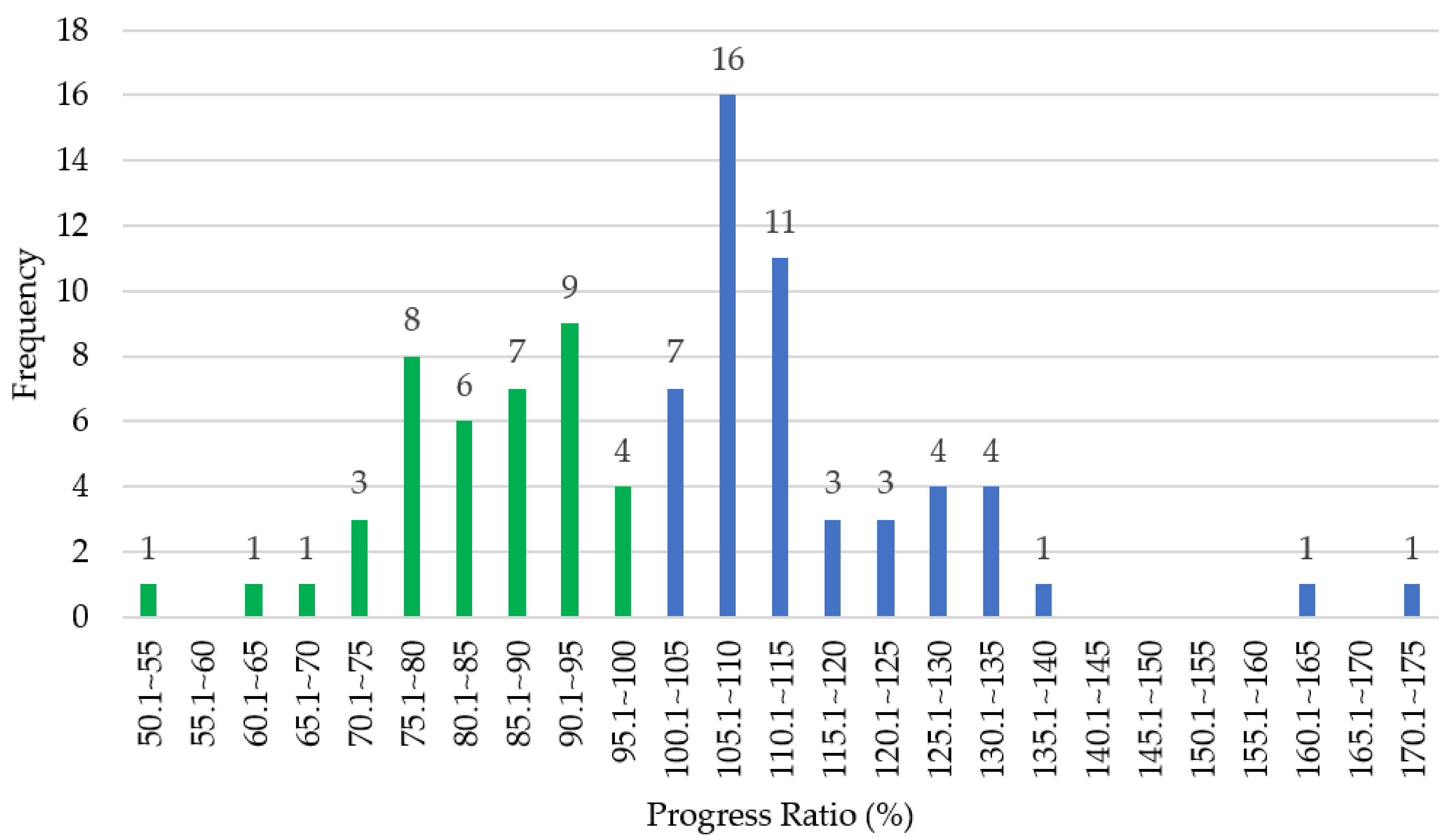
Figure 2 depicts a histogram of PRs for all 91 countries. The average PR was 101.50% with an SD of 20.11. On average, little change in the electricity productivity trend was observed from 1991 to 2011. Of the 91 countries, as many as 63 countries had their PRs ranging from 80% to 120%.
Further, 51 countries had a history of increasing EIs, whereas 40 countries experienced a decreasing trend. For the countries with an increasing trend, the average PR was 115.51% with an SD of 14.10. Although a few countries had very high PRs, exceeding 135%, 34 out of 51 countries had their PRs in the range of 100% to 115%. For the countries with a decreasing trend, the average PR was 83.64% with an SD of 9.74. Of the countries with decreasing PRs, 34 countries had PRs in the range of 75% to 100%, while six countries had very low PRs of below 75%.
5.1. Income Group Analysis
To examine whether income levels influence the trend of EIs, we divide the 91 countries into four subgroups based on income, following the World Bank classification (Table 2). Only the lower-middle income subgroup of 24 countries had a higher average PR, at 105.40%, than the average PR of 101.50% for the total sample of 91 countries. The other three income subgroups had their average PRs close to the 91 countries’ average PR.
Dividing the total sample into increasing and decreasing PR countries shows a different picture of the role that income levels play. Of the 51 countries with increasing PRs, only two countries in the low-income subgroup have substantially higher PRs (average PR: 147.27%) than the average PR of 51 countries (115.5%). The fact that the other three income subgroups (49 out of 51 countries) have their average PRs very close to the increasing PR group’s average of 115.5% means that the EI trends among the high-income, upper middle-income, and lower middle-income countries in the increasing PR group have little discernible difference.
Among the 40 countries with decreasing PRs, the high-income subgroup of 22 countries has an average PR of 88.16%, which is higher than the 40-country average. However, the remaining three subgroups have substantially lower PRs. This suggests that the high-income decreasing PR countries, on average, lagged behind the upper middle-, lower middle-, and low-income countries in terms of change in EI trend during the 1991–2011 period.
5.2. Regional Analysis
To examine the same types of questions for countries based on regional categorization, we formulate six regional subgroups by modifying the World Bank’s classification. The subgroups are East Asia and Pacific (EAP); Europe, Central Asia, and North America (ECANA) (North America is combined with Europe and Central Asia because the former has only two countries: the U.S. and Canada); Latin America and the Caribbean (LAC); the Middle East and North Africa (MENA); South Asia (SA); and Sub-Saharan Africa (SSA). The MENA subgroup of 16 countries displays a substantially higher PR of 106.61% than the average PR of our 91-country sample (101.5%), as illustrated in Table 3. The EAP and SA subgroups show average PRs of 104.46% and 103.59%, respectively, which are also relatively high.
As in the income group analysis, the average PR estimates of the increasing and decreasing PR groups depict a different picture than the total group of 91 countries. Among the 51 countries with increasing PRs, which have an average PR of 115.5%, the subgroups of SSA (eight countries) and ECANA (seven countries) display the highest and second highest PR, at 121.91% and 119.95%, respectively. By contrast, the LAC subgroup of 12 countries showed the lowest average PR of 109.06% in the increasing PR group. In the 40-country decreasing PR group, the ECANA subgroup of 12 countries displays the highest average PR of 88.73%; the EAP subgroup follows with an average PR of 87.41%. The lowest average PR is 76.02% for the SSA subgroup.
5.3. Population Analysis
As previous studies have documented the role played by population dynamics in energy related issues [52], further tests were conducted to examine the relationship between PR and three measures of population dynamics—population size, population density, and population growth rate during the 1991–2011 period. Population data were downloaded from the U.S. Census Bureau [53].
5.3.1. Population Size
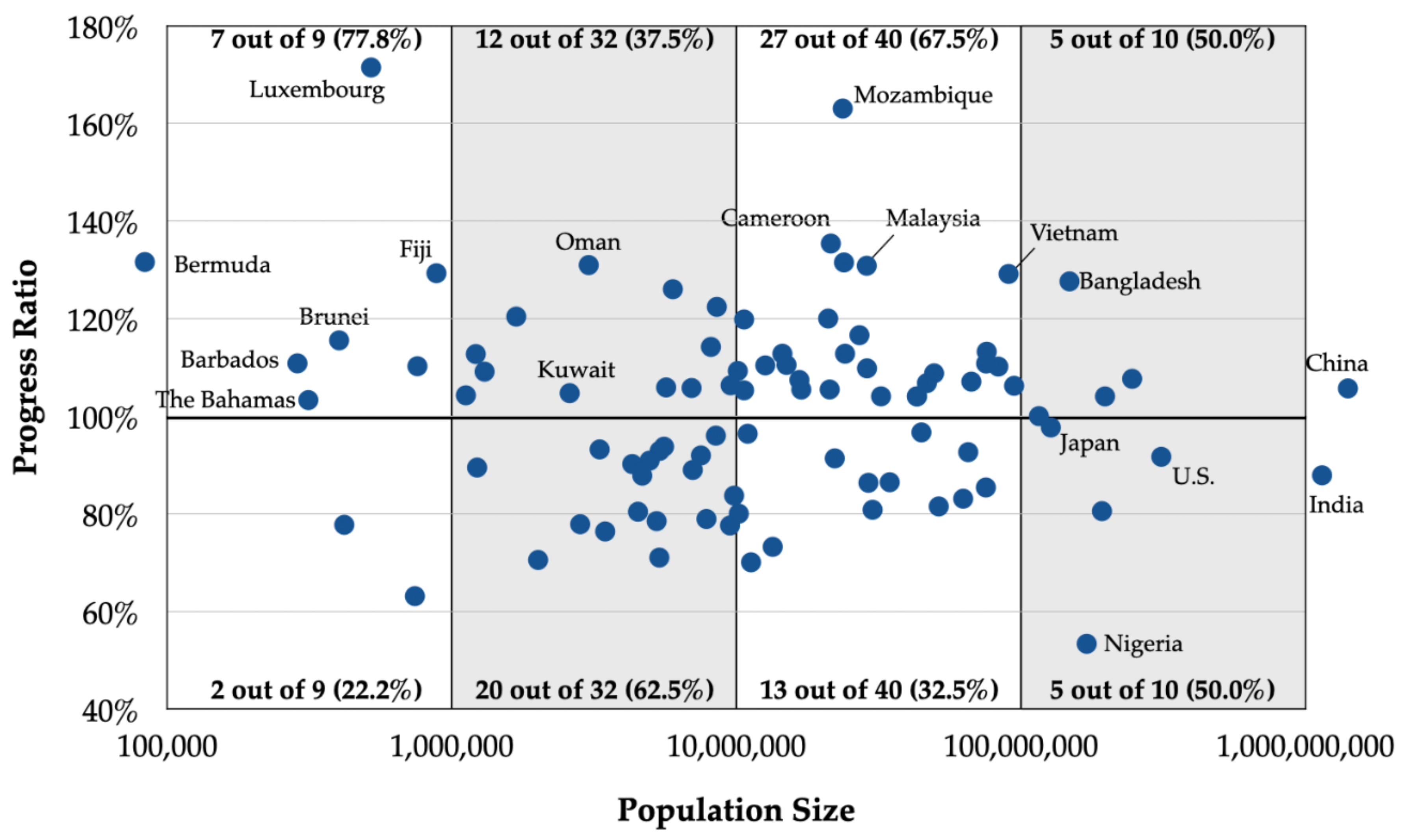
Figure 3 illustrates the fluctuations in the relationship between the population size of a country and the proportion of countries with an increasing slope. Increasing PR countries constitute 77.8% of the small population countries, 37.5% of countries with 1 to 10 million people, and 67.5% of the next group. The population size analysis suggests that the 32 increasing PR countries with a relatively large population of more than 10 million are most likely to contribute to a lower global average PR.
5.3.2. Population Density
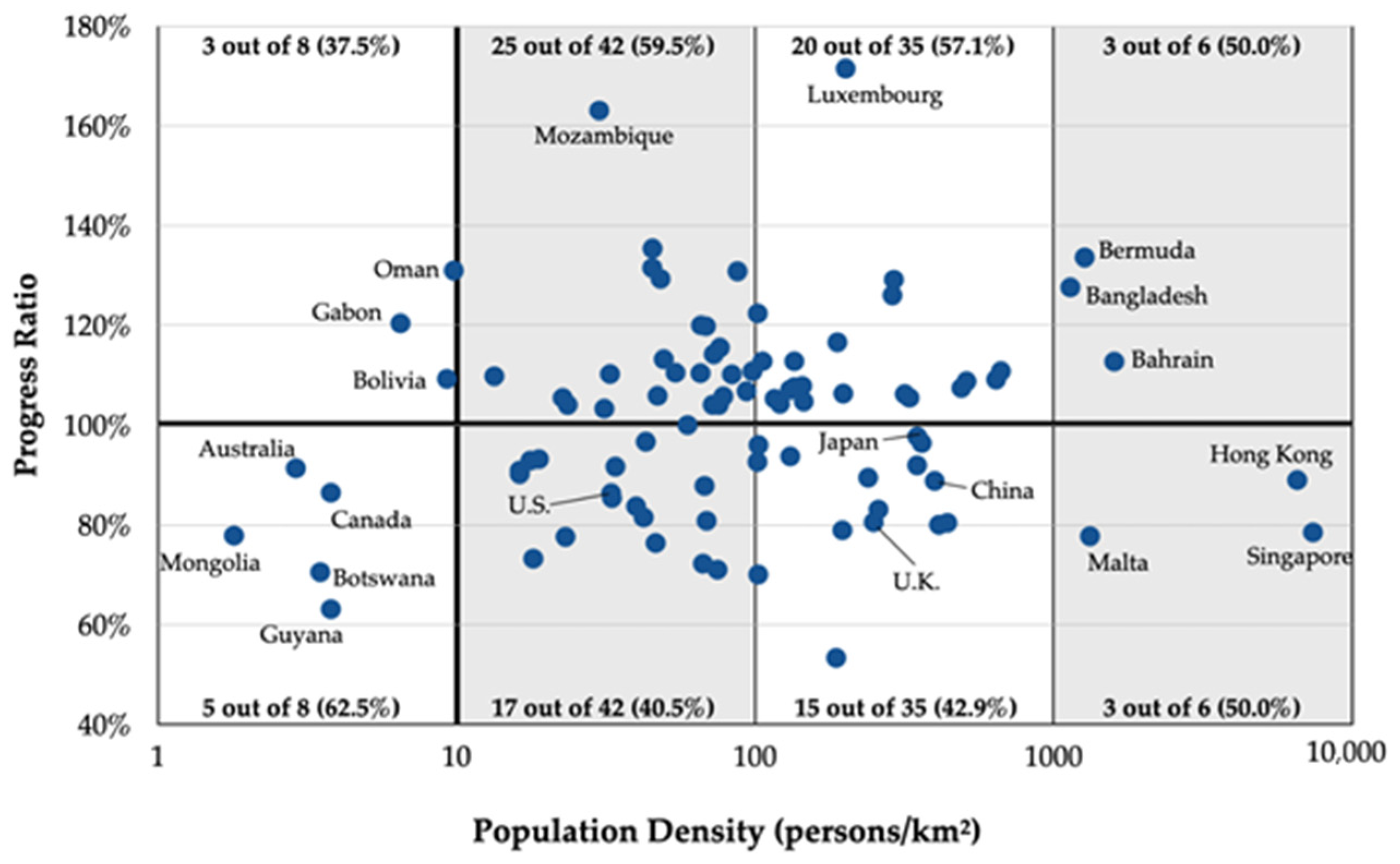
Figure 4 indicates that the proportion of countries with increasing slopes jumps from 37.5% (3 out of 8 countries) in the lowest population density group to 59.5% (25 out of 42 countries) in the group with 10–100 persons/km2. The proportion then gradually tapers off in the higher population density groups. Overall, population density has an impact on the proportion of increasing PR countries.
5.3.3. Population Growth Rate
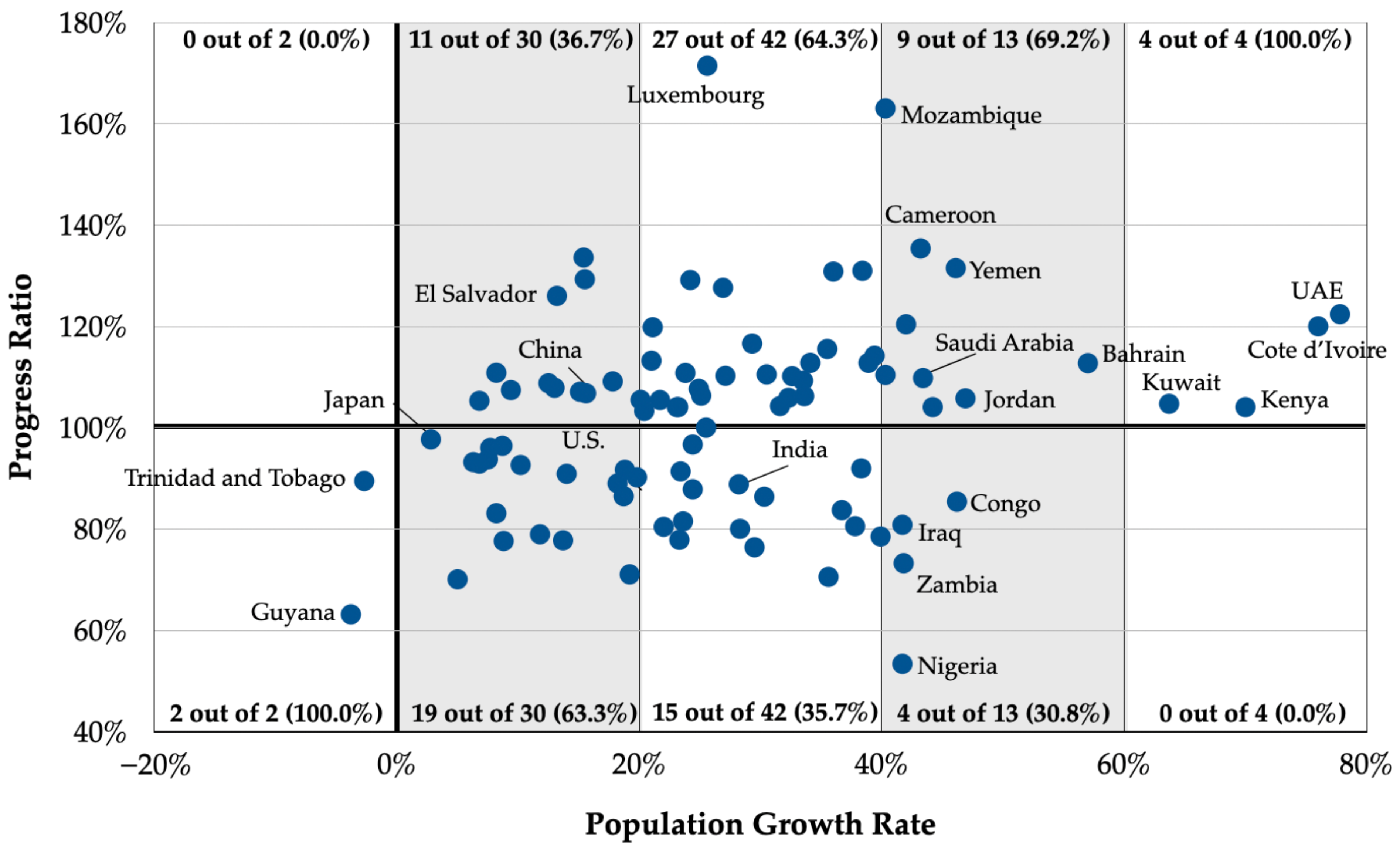
The population growth rate during the 1991–2011 period produced the most interesting results of the population dynamics. Figure 5 shows a clear pattern indicating that the proportion of increasing PR countries increases with a rapid expansion in the population size.
The group of countries with a population growth rate higher than 40% consists of only two regions, MENA and SSA. Combining these two rapid population growth groups shows 76.5% of the countries (13 out of 17) with increasing PRs. In general, high population growth appears to be associated with increasing slopes while low population growth tends to generate decreasing slopes.
5.4. Classical vs. Kinked
Finally, we examine the important question of which of the 91 countries are most likely to reverse their past trends and improve their EIs in the future. The 40 countries with a decreasing trend are less likely to make a breakthrough in the future because they have already made significant progress, as indicated by their average PR of 83.64%. This leaves the 51 countries with an increasing trend as possible candidates for improvement. Their average PR of 115.51%, which is higher than both the total group’s average of 101.50% and the decreasing group’s average of 83.64%, indicates the extent of possible improvement in the future. The 51-country group with an increasing trend comprises two subgroups: countries with classical experience slopes and those with kinked experience slopes. Table 4 demonstrates that 24 countries have increasing kinked slopes and 27 countries, increasing classical slopes. The average PR of the increasing kinked group, at 119.40%, is higher than that of the increasing classical group, at 112.05%. The table also shows that 27 countries have decreasing kinked slopes and 13 countries have decreasing classical slopes. The average PR of the decreasing kinked group, at 81.72%, is lower than that of the decreasing classical group, at 87.63%. Therefore, all four groups of countries need to be considered to answer the question about which groups are likely to make major improvements.
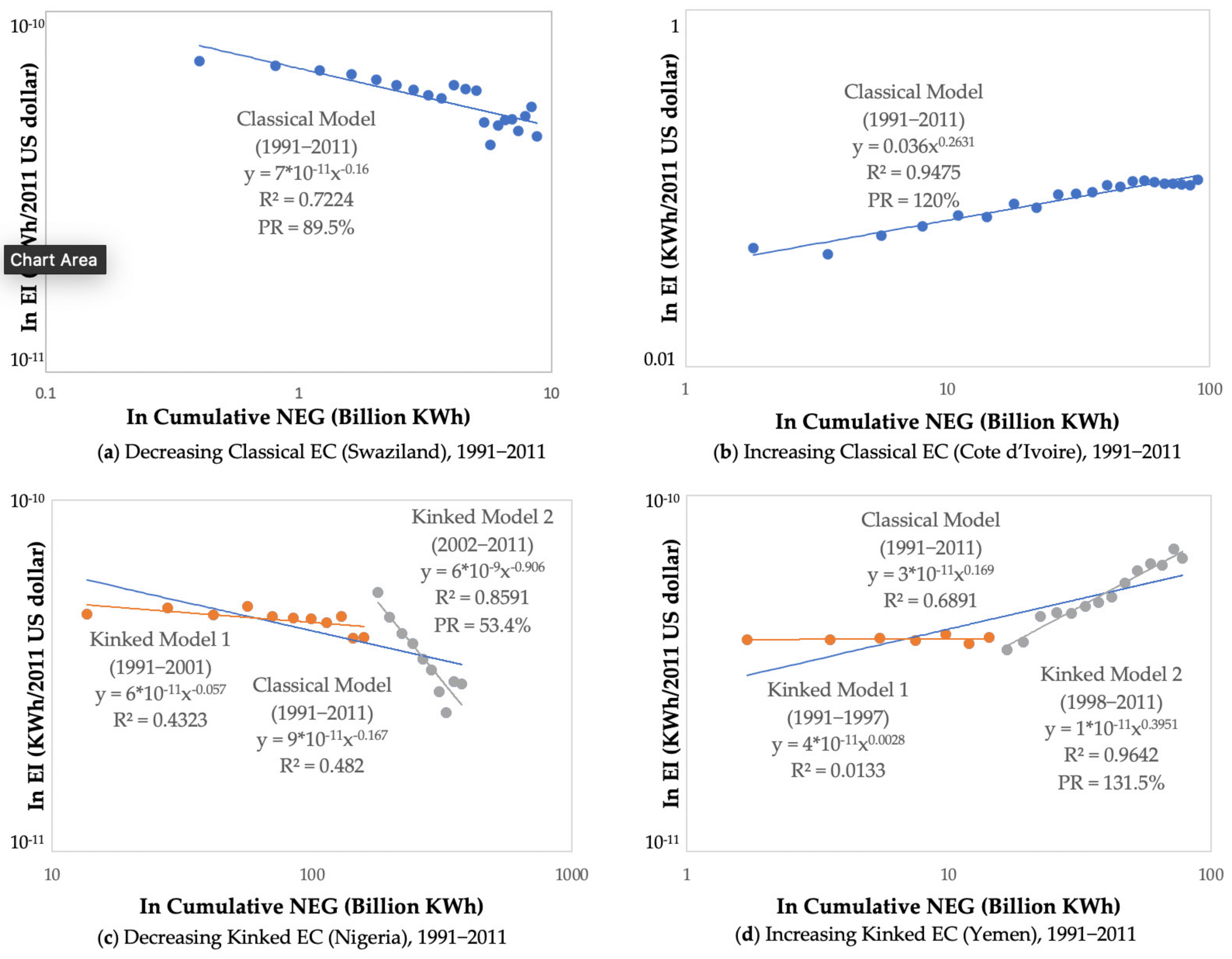
Figure 6 displays the EC diagram for representative countries from the four subgroups to explain the differences among the subgroups. Figure 6a,b shows a decreasing and an increasing classical EC for Swaziland and Côte d’Ivoire, respectively. The increasing classical slope for Côte d’Ivoire has a value of 0.2631, which translates into a PR of 120%. By contrast, the decreasing classical slope for Swaziland has a value of −0.16, which translates into a PR of 89.5%.
Figure 6c,d depicts a decreasing and an increasing kinked EC for Nigeria and Yemen, respectively. Nigeria displays two decreasing kinked slopes with the first covering the 1991⎼2001 period and the second, the 2002⎼2011 period. The second kinked slope has a steep value of −0.906, while the first slope has a value of −0.057. The second slope shows a PR of 53.36%. Yemen has two increasing kinked slopes with the first covering 1991⎼1997 and the second, 1998⎼2011. Once again, the second slope has a steeper value of 0.3951 compared to 0.0028 of the first slope. The second slope represents a PR of 131.50%.
In summary, a classical EC displays one slope for a given period, while a kinked EC displays two slopes for a given period. In general, the second kinked slope has a steeper value than the first slope. Only the second kinked slope is used to estimate the PR for a given country.
Now, we can make our selection from the four subgroups of countries presented in Table 4. We expect that the 27 countries with increasing classical slopes are most likely to switch their increasing classical slopes to decreasing kinked slopes in the future. These countries include Luxembourg (171.46%), Mozambique (163.04%), Côte d’Ivoire (120.01%), Brunei (115.54%), Iran (113.22%), and Turkey (110.8%).
Next are the 24 countries with increasing kinked slopes. These countries include Cameroon (135.38%), Bermuda (133.5%), Yemen (131.5%), Oman (130.97%), Malaysia (130.83%), and Vietnam (129.15%). This selection is made although the average PR of the increasing kinked group (119.4%) is higher than the average PR of the increasing classical group (112.05%). The increasing classical group is more likely than the increasing kinked group to switch to a decreasing kinked slope given the same degree of success in electricity resource management.
Finally, we should not overlook the decreasing classical subgroup of 13 countries. Although the average PR of this group is 87.63%, some countries could reduce their future PRs by converting their current classical decreasing slopes to steeper kinked decreasing slopes in the future. These countries could potentially include Columbia (96.68%), Belgium (96.41%), Austria (96.01%), Denmark (93.75%), Uruguay (93.19%), Finland (92.63%), and Norway (90.89%).
In sum, the maximum number of countries with the potential to improve their future PRs could exceed the 51 countries in the increasing PR group. In other words, depending on how effective their future management of electricity resources is, most of the 91 countries could improve their future EIs beyond what their past trends indicate.
5.5. Robustness Test
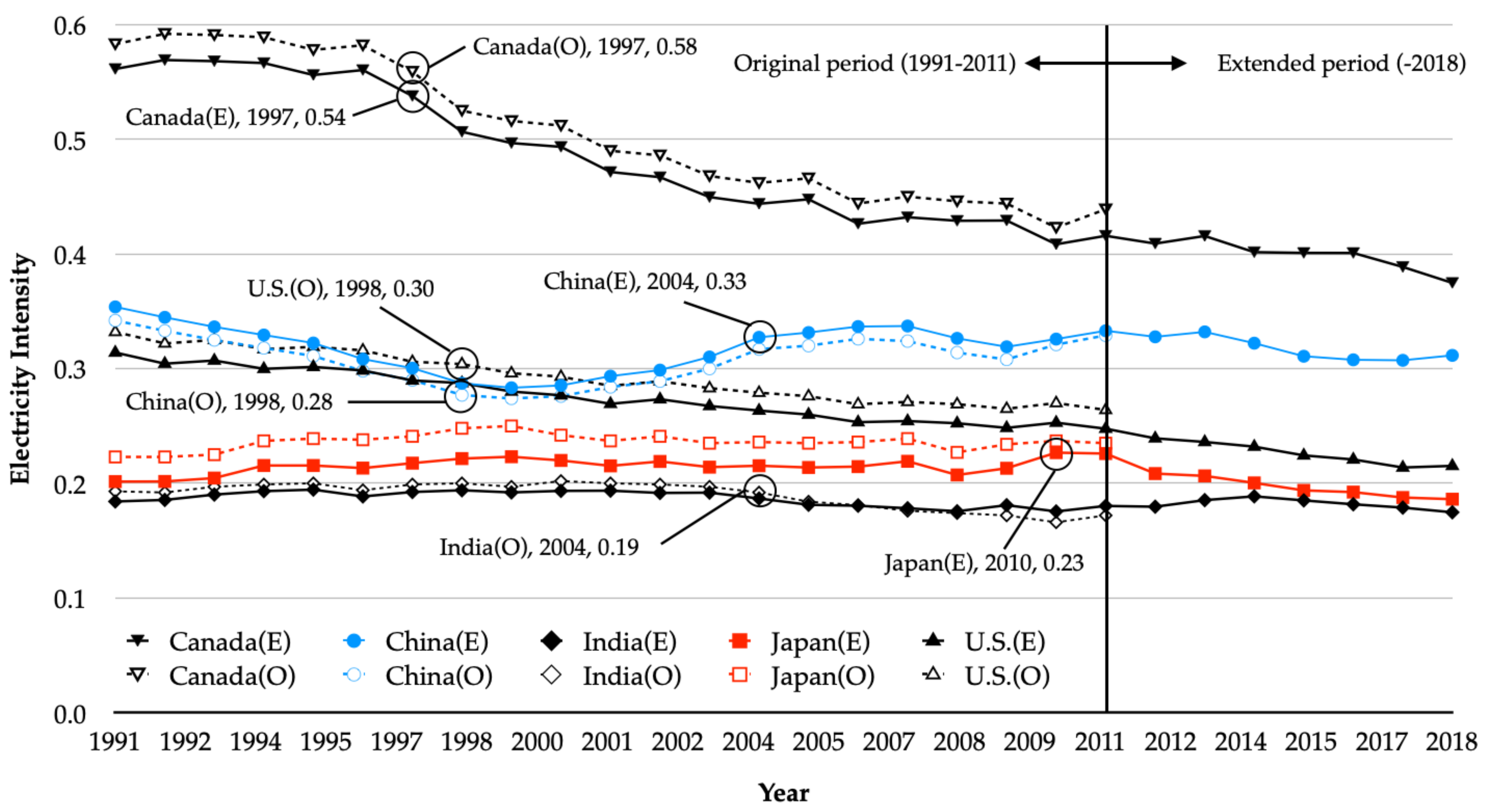
To check the robustness of the results, we conduct additional tests for the five largest producers of electricity—China, the U.S., Japan, India, and Canada—by using an updated dataset for the period from 1991 to 2018, which is the year for which the latest information is available. The NEG data have been downloaded from the EIA’s webpage on international energy statistics [44] and the GDP from the World Bank [54]. Figure 7 plots the historical change in EIs for five countries in the two datasets. Although we have employed the same analysis with an updated dataset, a comparison of the results from the original dataset (1991–2011) with those from the extended one (1991–2018) should be treated with caution because the GDP in the former is reported in 2011 constant dollars while that in the latter is based on 2015 constant dollars. While imperfect, the comparison is expected to provide some clues for the validity of our original investigation.
Table 5 reports the analysis for the five countries. The coefficients for all five countries meet the statistical test and the coefficients for three of the five countries display a switching slope between kinked and classical EC.
Canada’s ECs show virtually the same pattern in both datasets: the analysis with the updated dataset produces an EC with a decreasing slope kinked in 1997, same as that with the 1991–2011 dataset. The fact that the PR in both analyses is statistically significant with little change suggests that the country’s EI has kept improving at a similar pace even in the extended period from 2012 to 2018. An in-depth examination into the updated dataset reveals that Canada, which began to significantly improve its EI from 0.54 in 1997 to 0.42 in 2011, has maintained its pace of improvement even after 2011 with its EI reaching 0.38 in 2018.
India and the U.S. exhibit a pattern different from Canada. As in the case of Canada, the PRs of the two countries have a statistically significant and decreasing slope in the updated dataset as well as the original one. This indicates that both countries have maintained their trend of EI improvement even with seven more years added to the window of original data coverage. However, unlike the Canadian case, the ECs of the two countries change from a kinked curve with the original dataset to a classical one with the extended dataset.
In the case of the U.S., the EC with the original dataset is kinked in 1998, after which EI keeps improving from 0.30 in 1998 to 0.26 in 2011. In the extended dataset, EI improves from 0.29 in 1998 to 0.25 in 2011 and keeps improving, even in recent years, to reach 0.22 in 2018. This seems to have contributed to the shift from a kinked EC with the dataset through 2011 to a classical one with the dataset through 2018. As the difference in EIs before and after the kinked year is not as big as in the case of Canada, and the period in which the U.S. improves its EIs extends further into the 2010s, a classical EC now seems to be sufficient to capture EI changes during 1991–2018.
The reason for India’s shift from a kinked to a classical EC differs from that of the U.S. While India’s EI stays around 0.20 in the 1990s and improves from 2004 to reach 0.17 in 2008 in the original dataset, the extended period shows that EI again increases from 0.18 in 2011 to 0.19 in 2014 and then tapers off to 0.18 in 2018. This fluctuation in the added period at a level higher than the early 2000s makes the overall curve flatter than that in the period through 2011. Therefore, analysis with the updated dataset produces a classical EC with a PR of 99.8%.
A change in PR for China and Japan corroborates our prediction that countries with increasing PRs are more likely to make a breakthrough. In the case of China, the EC is kinked in 1998 with a PR of 107.9% in the original dataset but is kinked in 2004 with a PR of 99.5% in the extended dataset. That is, China’s EI stops deteriorating and is stabilized after 2004. Japan’s EC turns from classical, with a PR of 101.2% in the original dataset, to kinked in 2010, with a PR of 65.4% in the extended dataset. This dramatic change primarily results from the nationwide nuclear power plant shutdown after the Fukushima accident in 2011. Japan relied on nuclear power plants for approximately 30% of electricity generation up until 2011. As of March 2020, only nine reactors in five nuclear power plants in Japan are in operation [55].
Overall, the robustness test seems to support our forecast on the EI trend forward. The case of Canada and the U.S. fits well with our forecast that countries with decreasing PRs are less likely to make a breakthrough because they have already progressed significantly: both countries achieved significant progress earlier in the study period and maintained their improvement at the same pace thereafter. With improving EI since 2013 and as one of the increasing kinked slope countries, China is forecast as a good candidate to progress significantly. Japan also shows the forecast pattern to improve its EI; however, this is primarily caused by its accident, not by technological progress or policy changes. India is one country that seems to deviate from our forecast. While the country has maintained a downward slope even in the updated dataset, a PR of 99.8% suggests little change during the period: its EIs in the 2010s increased to the EI level of the 1990s and the early 2000s. A surge in electricity generation capacity during the early 2010s is believed to have contributed to the deterioration of EI: in coal-fired electricity generation alone, 78,440 MW of capacity was added between 2010 and 2014, increasing the country’s coal-fired electricity generation capacity to 164,953 MW [56].
6. Conclusions
The key points from the analysis of EI for 91 countries by using the EC are as follows. First, while previous studies reported the convergence of EI across countries, our findings demonstrated a wide variation in EI trends in a large sample of 91 countries. The PRs ranged from 53% to 135%, although the average PR of the sample at 101.5% suggests little change as a whole. This is useful information for policymakers as the results allow them to determine the current standing and the future direction of their respective countries in terms of EI trends.
Second, we illustrated that more than half of the countries in the dataset experienced a significant change—a kink—in their PR trends. This has not been reported in previous studies. Out of the 20 lowest PR countries, 16 countries experienced a downward kink. The factors that contributed to the kink are worth investigating. At the same time, out of the 20 highest PR countries, 15 countries experienced an upward kink, the reasons for which need to be investigated. Both cases suggest that EI is susceptible to a sudden change in trend, for better or worse. In future EI analyses, both academic researchers and energy policymakers should closely focus on the countries with fluctuating PR trends.
Third, the results showed that the five major NEG countries contributed to the improvement of the world’s electricity productivity as their average PR was 94.27%. Out of the five countries, Canada displayed the lowest PR of 86.36%. However, this may result from a relatively high level of its EI in the early 1990s, with its latest EI being still higher than that of the other four countries. To catch up with the EI level of these countries, Canada needs to step up its efforts to reduce EI and achieve the second kink in the near future. By contrast, China is the only country among the five major NEG countries to have an increasing PR of 107.87%, although its overall EI is at a lower level than that of Canada. China experienced a kink in 1998 with a decreasing PR of 99.44% until 1997 and an increasing PR of 107.87% since 1998. Considering its importance in the global economy, China needs to improve its EI in the near future. Fortunately, in the robustness test with the extended period up to 2018, China’s EI showed a drop and a downward trend since 2013. As the five countries play an important role in the global economy, it is important for them to take one further step to improve their EIs in the future. Otherwise, efforts to enhance the global welfare, such as the United Nation’s Sustainable Development Goals, will not produce meaningful results.
Fourth, the analysis of the income and regional subgroups did not yield discernible patterns of relationship with a country’s PR. However, one of the population related variables, population growth rate, produced a clear pattern: the higher the rate of population growth, the higher the proportion of countries that exhibit an increasing PR. As a category analysis, the result only suggests a plausible pattern between the rate of population growth and PR. In future research, the factors influencing population growth rates, such as structural changes in the economy, technological changes, and government regulations, should be further investigated.
Fifth, we selected 27 countries that displayed classical experience slopes with increasing PR trends. This group included countries such as Luxembourg (171.46%), Mozambique (163.04%), Côte d’Ivoire (120.01%), Brunei (115.54%), and Iran (113.22%). Other countries with increasing PR trends and kinked experience slopes represented the second potential group and included Cameroon (135.38%), Bermuda (133.59%), Yemen (131.50%), Oman (130.97%), and Malaysia (130.83%).
Based on the aforementioned findings, our study provides several policy implications. First, given our results for 91 countries, the policymakers can analyze their respective country’s performance. In particular, more than half of the countries we examined in this study exhibited PRs of more than 100%. These countries may need to take active steps to improve the productivity of electricity generation. For instance, emphasizing the service and commercial sectors over the electricity-intensive manufacturing sector may help. Adopting a cost-efficient technology for electricity generation would be another solution. These countries may obtain fruitful insights by benchmarking better-performing countries with similar economic or environmental characteristics. Finally, our analysis adopted two types of ECs: classical and kinked. This can enable the countries that experienced fluctuating rates of changes, or are likely to experience a significant shift in EI, to adopt appropriate reduction targets.
Our study has several limitations involving both conceptual and technical issues, which warrant further research. Conceptually, EI, as used in this study, is a vast simplification of a complex relationship that exists between electricity generation and GDP [57,58]. Therefore, future research may include various economic variables, such as growth rate or stage of economic development. Additionally, the sources of electricity generation may be another important aspect to consider. Finally, each country’s structural differences in electricity consumption, including the type of major industries, buildings, and transportation systems, as well as environmental factors (e.g., weather), also need to be examined.
At a technical level, the model used in this study is a simple aggregate EC that is only driven by a single independent variable of cumulative NEG, which leaves room for further refinement. One approach that may extend the current research is the adoption of the environmental Kuznets curve (EKC), which hypothesizes an inverted U-shaped relationship between environmental degradation, such as CO2 emission and per capita income [59,60]. To elaborate, the traditional EKC studies have been expanded to analyze the relationship between pollution emissions, economic growth and energy consumption because emissions are primarily generated by energy consumption [61,62,63]. Lean and Smyth [64] have used electricity consumption to represent energy usage from five ASEAN countries using the same type of model and found that a one percent increase in electricity consumption per capita was associated with an increase in CO2 emissions per capita at 0.511% from the panel. The elasticity of CO2 emissions per capita to real GDP per capita was 3.106–0.404 GDP per capita at the threshold income, supporting the EKC hypothesis that the emissions declined following the threshold income level. An interesting extension of this research might be to relate countries with four different experience slopes of increasing classical, increasing kinked, decreasing classical, and decreasing kinked to dynamic changes of real GDP per capita to test the EKC hypothesis.
In short, our study should be viewed as a modest beginning to better understand the wide variation in the EIs trends among several countries. Future studies incorporating the factors affecting a country’s economic performance, electricity generation, and consumption can elucidate the reasons for the wide variation in EIs among multiple countries.
Author Contributions
The authors contributed to the development, implementation, analysis, and writing of this study as follows: conceptualization, methodology, and analysis—Y.-S.C. and H.-E.K.; original draft preparation—Y.-S.C. and H.-E.K.; review and editing—Y.-S.C., H.-J.K., and H.-E.K. All authors have read and agreed to the published version of the manuscript.
Funding
This research received no external funding.
Institutional Review Board Statement
Not applicable.
Informed Consent Statement
Not applicable.
Data Availability Statement
Publicly available datasets were analyzed in this study.
Acknowledgments
We thank So Young Yang for her capable assistance during the research.
Conflicts of Interest
The authors declare no conflict of interest.
Appendix A

Table A1.
Results of classical and kinked experience curve analysis of EI for 91 countries.
| Country | Classical Experience Equation | Kinked Year | Kinked Experience Equation | Model Selection | |||||||||
|---|---|---|---|---|---|---|---|---|---|---|---|---|---|
| ln a | b | R2 | PR | ln a1 | b1 | ln a2 | b2 | b2-b1 | R2 | PR2 | |||
| 1. Nigeria | −23.115 ** (0.296) | −0.167 * (0.060) | 0.4820 | 0.8909 | 2002 | −23.563 ** (0.190) | −0.057 (0.043) | −18.993 ** (0.987) | −0.906 ** (0.181) | −0.849 ** (0.186) | 0.8591 | 0.5336 | Kinked |
| 2. Guyana | −1.981 ** (0.097) | 0.171 ** (0.050) | 0.4010 | 1.1256 | 2001 | −1.984 ** (0.109) | 0.374 ** (0.101) | −0.161 (0.199) | −0.664 ** (0.089) | −1.037 ** (0.135) | 0.8633 | 0.6313 | Kinked |
| 3. Cuba | −1.825 ** (0.342) | −0.098 (0.069) | 0.2950 | 0.9345 | 2000 | −2.539 ** (0.150) | 0.093 ** (0.036) | 0.358 (0.290) | −0.513 ** (0.053) | −0.607 ** (0.064) | 0.9480 | 0.7006 | Kinked |
| 4. Botswana | −2.067 ** (0.472) | −0.504 * (0.206) | 0.6270 | 0.7054 | 2001 | −2.436 ** (0.305) | −0.187 (0.170) | 1.831 (0.931) | −0.187 (0.170) | −1.820 ** (0.401) | 0.8948 | 0.8784 | Classical |
| 5. Sierra Leone | −24.412 ** (0.104) | −0.494 * (0.182) | 0.3620 | 0.7103 | 2005 | −24.294 ** (0.090) | −0.295 (0.156) | −27.038 ** (1.235) | 2.789 (1.587) | 3.084 (1.594) | 0.6636 | 6.9120 | Classical |
| 6. Zambia | −21.005 ** (0.246) | −0.197 ** (0.055) | 0.7518 | 0.8724 | 1999 | −21.472 ** (0.126) | −0.053 (0.037) | −19.816 ** (0.134) | −0.449 ** (0.028) | −0.397 ** (0.056) | 0.9569 | 0.7323 | Kinked |
| 7. Panama | −22.656 ** (0.072) | −0.001 (0.021) | 0.0001 | 0.9994 | 2002 | −22.795 ** (0.129) | 0.0520 (0.044) | −21.009 ** (0.187) | −0.389 ** (0.044) | −0.441 ** (0.062) | 0.6315 | 0.7638 | Kinked |
| 8. Sweden | 0.442 (0.351) | −0.177 ** (0.048) | 0.7608 | 1.1307 | 1999 | −0.361 (0.185) | −0.045 (0.029) | 1.866 ** (0.387) | −0.366 ** (0.050) | −0.321 ** (0.057) | 0.9403 | 0.7761 | Kinked |
| 9. Malta | −22.256 ** (0.212) | −0.039 ** (0.011) | 0.3220 | 0.9732 | 2003 | −22.229 ** (0.030) | −0.061 ** (0.014) | −21.142 ** (0.363) | −0.363 ** (0.064) | −0.303 ** (0.066) | 0.8722 | 0.7774 | Kinked |
| 10. Mongolia | −21.684 ** (0.075) | −0.154 ** (0.023) | 0.8365 | 0.8989 | 2000 | −21.757 ** (0.103) | −0.127 ** (0.038) | −20.900 ** (0.138) | −0.361 ** (0.038) | −0.234 ** (0.054) | 0.9535 | 0.7786 | Kinked |
| 11. Singapore | −22.536 ** (0.065) | −0.033* (0.014) | 0.1616 | 0.9777 | 2001 | −22.643 ** (0.099) | −0.011 (0.022) | −20.614 ** (0.227) | −0.349 ** (0.037) | −0.338 ** (0.043) | 0.8794 | 0.7850 | Kinked |
| 12. Switzerland | −22.003 ** (0.270) | −0.078 (0.042) | 0.3849 | 0.9475 | 1999 | −22.452 ** (0.229) | 0.007 (0.041) | −20.167 ** (0.265) | −0.349 ** (0.039) | −0.356 ** (0.057) | 0.8078 | 0.7851 | Kinked |
| 13. Rwanda | −24.501 ** (0.109) | −0.341* (0.148) | 0.3546 | 0.7894 | 2000 | −24.168 ** (0.123) | 0.022 (0.138) | −25.322 ** (0.241) | 0.523 (0.257) | 0.500 (0.292) | 0.7793 | 1.4364 | Classical |
| 14. Lebanon | −2.469 ** (0.092) | 0.207 ** (0.025) | 0.7757 | 1.1541 | 2002 | −2.679 ** (0.082) | 0.281 ** (0.025) | 0.081 (0.385) | −0.321 ** (0.080) | −0.602 ** (0.084) | 0.9539 | 0.8003 | Kinked |
| 15. Pakistan | −22.960 ** (0.102) | 0.033 (0.017) | 0.2038 | 1.0230 | 2007 | −23.172 ** (0.054) | 0.073 ** (0.009) | −20.553 ** (0.542) | −0.314 * (0.075) | −0.387 ** (0.054) | 0.0310 | 0.8042 | Kinked |
| 16. Iraq | −0.309 (0.211) | −0.312 ** (0.039) | 0.7620 | 0.8054 | 1998 | −0.701* (0.275) | −0.202 ** (0.063) | −2.358 ** (0.537) | 0.025 (0.090) | 0.227 (0.110) | 0.9016 | 1.0174 | Classical |
| 17. South Africa | −21.240 ** (0.179) | −0.042 (0.024) | 0.3366 | 0.9711 | 2005 | −21.528 ** (0.090) | 0.002 (0.013) | −19.118 ** (0.264) | −0.307 ** (0.033) | −0.309 ** (0.035) | 0.8695 | 0.8082 | Kinked |
| 18. U.K. | −0.932 ** (0.162) | −0.101 ** (0.020) | 0.8038 | 0.9323 | 2002 | −1.273 ** (0.061) | −0.053 ** (0.008) | 0.719* (0.285) | −0.295 ** (0.033) | −0.242 ** (0.034) | 0.9786 | 0.8151 | Kinked |
| 19. Guinea | −2.694 ** (0.046) | 0.049* (0.023) | 0.2104 | 1.0345 | 2001 | −2.690 ** (0.049) | 0.007 (0.046) | −1.909 ** (0.116) | −0.267 ** (0.046) | −0.274 ** (0.065) | 0.7217 | 0.8309 | Kinked |
| 20. Congo (Kinshasa) | −2.179 ** (0.147) | 0.149 ** (0.038) | 0.5564 | 1.1085 | 2000 | −2.213 ** (0.278) | 0.150 (0.083) | −0.339 (0.350) | −0.256 ** (0.078) | −0.406 ** (0.114) | 0.8463 | 0.8372 | Kinked |
| 21. Venezuela | −22.737 ** (0.082) | 0.085 ** (0.014) | 0.5895 | 1.0604 | 2002 | −22.713 ** (0.147) | 0.078 ** (0.025) | −20.474 ** (0.642) | −0.228* (0.088) | −0.306 ** (0.091) | 0.8760 | 0.8539 | Kinked |
| 22. Canada | 0.363 (0.298) | −0.124 ** (0.034) | 0.8093 | 0.9175 | 1997 | −0.504 ** (0.117) | −0.004 (0.015) | 1.136 ** (0.152) | −0.212 ** (0.017) | −0.207 ** (0.023) | 0.9854 | 0.8636 | Kinked |
| 23. Ireland | −1.141 ** (0.176) | −0.154 ** (0.033) | 0.8500 | 0.8985 | 1994 | −1.744 ** (0.101) | 0.019 (0.029) | −0.839 ** (-0.210) | −0.210 ** (0.018) | −0.229 ** (0.034) | 0.9390 | 0.8647 | Kinked |
| 24. India | −1.364 ** (0.145) | −0.037 (0.018) | 0.3497 | 0.9750 | 2004 | −1.717 ** (0.028) | 0.013 ** (0.004) | −0.027 (0.527) | −0.187* (0.058) | −0.200 ** (0.058) | 0.9540 | 0.8782 | Kinked |
| 25. Hong Kong | −1.067 ** (0.168) | −0.171 ** (0.028) | 0.7186 | 0.8882 | 1994 | −1.707 ** (0.367) | 0.006 (0.086) | −1.426 ** (0.245) | −0.112* (0.042) | −0.118 (0.096) | 0.8235 | 0.9256 | Classical |
| 26. Trinidad and Tobago | −21.881 ** (0.158) | −0.103* (0.040) | 0.5539 | 0.9311 | 1999 | −22.210 ** (0.082) | 0.034 (0.028) | −21.624 ** (0.300) | −0.168* (0.074) | −0.203 * (0.079) | 0.8287 | 0.8899 | Kinked |
| 27. Swaziland | −23.391 ** (0.042) | −0.161 ** (0.030) | 0.7224 | 0.8947 | 2003 | −23.408 ** (0.012) | −0.091 ** (0.014) | −23.987 ** (0.469) | 0.122 (0.247) | 0.213 (0.247) | 0.8998 | 1.0885 | Classical |
| 28. New Zealand | −0.422 ** (0.090) | −0.111 ** (0.015) | 0.8979 | 0.9261 | 1999 | −0.678 ** (0.041) | −0.055 ** (0.008) | −0.192 (0.156) | −0.149 ** (0.025) | −0.094 ** (0.026) | 0.9735 | 0.9020 | Kinked |
| 29. Norway | 0.182 (0.187) | −0.138 ** (0.026) | 0.6848 | 0.9089 | 2003 | 0.021 (0.243) | −0.110 ** (0.037) | −1.518 (1.310) | 0.083 (0.171) | 0.193 (0.175) | 0.7485 | 1.0593 | Classical |
| 30. Australia | −0.872 ** (0.014) | −0.051 ** (0.106) | 0.5962 | 0.9650 | 2005 | −1.098 ** (0.0400) | −0.016* (0.006) | −0.265 (0.161) | −0.130 ** (0.020) | −0.114 ** (0.051) | 0.9477 | 0.9136 | Kinked |
| 31. U.S.A. | −0.394* (0.149) | −0.081 ** (0.014) | 0.8889 | 0.9452 | 1997 | −0.898 ** (0.064) | −0.026 ** (0.007) | 0.078 (0.069) | −0.125 ** (0.007) | −0.100 ** (0.009) | 0.9877 | 0.9168 | Kinked |
| 32. Israel | −1.449 ** (0.063) | 0.008 (0.011) | 0.0392 | 1.0056 | 2002 | −1.430 ** (0.110) | 0.003 (0.021) | −0.619 ** (0.162) | −0.121 ** (0.025) | −0.124 ** (0.033) | 0.3740 | 0.9195 | Kinked |
| 33. France | −1.065 ** (0.162) | −0.044* (0.019) | 0.5357 | 0.9700 | 1996 | −1.531 ** (0.034) | 0.021 ** (0.005) | −0.483 ** (0.100) | −0.110 ** (0.012) | −0.132 ** (0.013) | 0.8952 | 0.9263 | Kinked |
| 34. Finland | −0.259 (0.196) | −0.106 ** (0.030) | 0.6204 | 0.9290 | 2005 | −0.531 ** (0.134) | −0.056* (0.022) | −0.313 (2.078) | −0.106 (0.292) | −0.050 (0.293) | 0.8012 | 0.9293 | Classical |
| 35. Uruguay | −21.917 ** (0.168) | −0.102* (0.040) | 0.2035 | 0.9319 | 2004 | −22.178 ** (0.205) | −0.038 (0.057) | −24.568 ** (1.618) | 0.414 (0.324) | 0.453 (0.329) | 0.3740 | 1.3326 | Classical |
| 36. Denmark | −1.226 ** (0.218) | −0.093* (0.036) | 0.2931 | 0.9375 | 1996 | −1.669* (0.727) | −0.004 (0.153) | 0.200 (0.584) | −0.323 ** (0.092) | −0.318 (0.179) | 0.6285 | 0.7997 | Classical |
| 37. Austria | −1.330 ** (0.090) | −0.059 ** (0.015) | 0.6633 | 0.9601 | 2002 | −1.503 ** (0.034) | −0.025 ** (0.006) | −1.170 (0.519) | −0.084 (0.077) | −0.060 (0.077) | 0.8099 | 0.9432 | Classical |
| 38. Belgium | −1.260 ** (0.083) | −0.053 ** (0.013) | 0.5839 | 0.9641 | 2001 | −1.497 ** (0.051) | −0.008 (0.009) | −1.249 ** (0.333) | −0.056 (0.048) | −0.048 (0.049) | 0.8041 | 0.9617 | Classical |
| 39. Colombia | −1.788 ** (0.129) | −0.049* (0.021) | 0.4082 | 0.9668 | 1993 | −1.124 ** (0.322) | −0.239 (0.084) | −1.527 ** (0.145) | −0.090 ** (0.023) | 0.149 (0.088) | 0.7763 | 0.9393 | Classical |
| 40. Japan | −1.585 ** (0.077) | 0.017* (0.008) | 0.2050 | 1.0116 | 2000 | −1.884 ** (0.156) | 0.054* (0.018) | −1.120 ** (0.170) | −0.034* (0.017) | −0.087 ** (0.026) | 0.7696 | 0.9769 | Classical |
| 41. Mexico | −2.180 ** (0.019) | 0.000 ** (0.000) | 0.8537 | 1.0001 | 1995 | −2.230 ** (0.026) | 0.000 (0.000) | −2.124 ** (0.009) | 0.000 ** (0.000) | −0.000 (0.000) | 0.9674 | 1.0001 | Classical |
| 42. Bahamas | −1.703 ** (0.027) | 0.047 ** (0.014) | 0.3678 | 1.0330 | 2007 | −1.737 ** (0.023) | 0.068 ** (0.010) | 1.186 (1.331) | −0.825 (0.392) | −0.893* (0.392) | 0.7425 | 0.5646 | Classical |
| 43. Brazil | −2.254 ** (0.061) | 0.057 ** (0.008) | 0.8176 | 1.0406 | 1997 | −2.011 ** (0.095) | 0.019 (0.015) | −2.211 ** (0.133) | 0.053 ** (0.016) | 0.034 (0.021) | 0.8814 | 1.0372 | Classical |
| 44. Kenya | −2.896 ** (0.021) | 0.057 ** (0.006) | 0.6515 | 1.0406 | 1999 | −2.929 ** (0.069) | 0.075 ** (0.024) | −3.153 ** (0.178) | 0.117* (0.042) | 0.043 (0.048) | 0.7518 | 1.0846 | Classical |
| 45. Morocco | −23.282 ** (0.085) | 0.058 ** (0.017) | 0.4572 | 1.0407 | 1995 | −23.373 ** (0.157) | 0.073 (0.049) | −22.917 ** (0.139) | -0.013 (0.027) | −0.087 (0.056) | 0.7084 | 0.9908 | Classical |
| 46. Cyprus | −2.042 ** (0.051) | 0.061 ** (0.014) | 0.5516 | 1.0428 | 1995 | −2.011 ** (0.033) | 0.075 ** (0.026) | −2.324 ** (0.049) | 0.137 ** (0.012) | 0.062 (0.030) | 0.9152 | 1.0998 | Classical |
| 47. Kuwait | −1.968 ** (0.130) | 0.067* (0.024) | 0.4558 | 1.0472 | 2005 | −2.065 ** (0.261) | 0.090 (0.051) | −3.733 ** (0.869) | 0.343 (0.139) | 0.253 (0.148) | 0.6283 | 1.2683 | Classical |
| 48. Portugal | −2.305 ** (0.081) | 0.075 ** (0.015) | 0.7145 | 1.0530 | 2007 | −2.277 ** (0.078) | 0.069 ** (0.014) | −6.448* (1.964) | 0.704 (0.297) | 0.635* (0.298) | 0.8478 | 1.6286 | Classical |
| 49. Chile | −2.204 ** (0.131) | 0.077 ** (0.022) | 0.7462 | 1.0546 | 1999 | −1.913 ** (0.221) | 0.020 (0.046) | −1.938 ** (0.036) | 0.036 (0.027) | 0.017 (0.053) | 0.8923 | 1.0255 | Classical |
| 50. Sri Lanka | −2.975 ** (0.064) | 0.077 ** (0.017) | 0.6439 | 1.0548 | 2005 | −3.046 ** (0.104) | 0.102 ** (0.028) | −1.431 (0.690) | −0.255 (0.143) | −0.357* (0.146) | 0.8216 | 0.8379 | Classical |
| 51. Jordan | −2.020 ** (0.042) | 0.081 ** (0.010) | 0.8435 | 1.0578 | 2007 | −1.986 ** (0.039) | 0.069 ** (0.011) | −0.999* (0.239) | −0.120 (0.049) | −0.189 ** (0.050) | 0.9037 | 0.9203 | Classical |
| 52. Nicaragua | −22.973 ** (0.033) | 0.083 ** (0.012) | 0.6595 | 1.0589 | 2002 | −22.895 ** (0.057) | 0.035 (0.024) | −22.899 ** (0.300) | 0.068 (0.085) | 0.033 (0.088) | 0.7868 | 1.0483 | Classical |
| 53. Philippines | −23.331 ** (0.108) | 0.087 ** (0.019) | 0.6051 | 1.0623 | 2005 | −23.587 ** (0.157) | 0.142 ** (0.028) | −21.936 ** (0.515) | −0.132 (0.077) | −0.275 ** (0.082) | 0.9001 | 0.9123 | Classical |
| 54. Dominican Republic | −2.450 ** (0.087) | 0.089 ** (0.026) | 0.3591 | 1.0633 | 2002 | −2.555 ** (0.109) | 0.119 ** (0.032) | 0.482 ** (0.509) | −0.510 (0.102) | −0.628 ** (0.107) | 0.8744 | 0.7024 | Classical |
| 55. Spain | −2.300 ** (0.101) | 0.073 ** (0.013) | 0.8723 | 1.0515 | 1996 | −1.933 ** (0.063) | 0.011 (0.010) | −2.473 ** (0.080) | 0.095 ** (0.010) | 0.084 ** (0.014) | 0.9492 | 1.0679 | Kinked |
| 56. Thailand | −23.265 ** (0.045) | 0.099 ** (0.007) | 0.9014 | 1.0708 | 1998 | −23.272 ** (0.118) | 0.097 ** (0.021) | −22.726 ** (0.124) | 0.023 (0.018) | −0.074* (0.028) | 0.9700 | 1.0163 | Classical |
| 57. Netherlands | −1.840 ** (0.063) | −0.024* (0.011) | 0.1769 | 0.9837 | 1999 | −1.8880 ** (0.091) | -0.012 (0.016) | −2.750 ** (0.212) | 0.103 ** (0.031) | 0.116 ** (0.035) | 0.6489 | 1.0742 | Kinked |
| 58. Indonesia | −3.757 ** (0.222) | 0.164 ** (0.032) | 0.7854 | 1.1207 | 1998 | −2.966 ** (0.130) | -0.001 (0.028) | −3.324 ** (0.239) | 0.107 ** (0.033) | 0.107* (0.044) | 0.9678 | 1.0766 | Kinked |
| 59. China | −1.106 ** (0.159) | −0.008 (0.017) | 0.0179 | 0.9944 | 1998 | −0.594 ** (0.181) | -0.071 ** (0.023) | −2.260 ** (0.136) | 0.109 ** (0.014) | 0.180 ** (0.027) | 0.8337 | 1.0787 | Kinked |
| 60. Korea, South | −2.214 ** (0.059) | 0.121 ** (0.007) | 0.9393 | 1.0878 | 1994 | −1.951 ** (0.115) | 0.066 ** (0.021) | −2.026 ** (0.052) | 0.098 ** (0.006) | 0.032 (0.022) | 0.9693 | 1.0701 | Classical |
| 61. Mauritius | −23.169 ** (0.067) | 0.126 ** (0.023) | 0.6691 | 1.0913 | 2000 | −23.066 ** (0.032) | 0.010 (0.034) | −22.799 ** (0.100) | 0.017 (0.032) | 0.006 (0.046) | 0.9128 | 1.0115 | Classical |
| 62. Saudi Arabia | −23.500 ** (0.079) | 0.135 ** (0.012) | 0.9140 | 1.0980 | 2004 | −23.683 ** (0.131) | 0.167 ** (0.020) | −22.967 ** (0.392) | 0.062 (0.052) | −0.105 (0.056) | 0.9618 | 1.0440 | Classical |
| 63. Bolivia | −2.629 ** (0.067) | 0.017 ** (0.019) | 0.9100 | 1.0121 | 1994 | −2.424 ** (0.000) | −0.028 ** (0.000) | −2.704 ** (0.030) | 0.128 ** (0.009) | 0.156 ** (0.009) | 0.9695 | 1.0927 | Kinked |
| 64. Egypt | −2.634 ** (0.150) | 0.114 ** (0.023) | 0.7946 | 1.0825 | 2000 | −2.168 ** (0.060) | 0.021 (0.012) | −2.789 ** (0.171) | 0.140 ** (0.025) | 0.119 ** (0.028) | 0.8302 | 1.1017 | Kinked |
| 65. Djibouti | −2.174 ** (0.018) | 0.141 ** (0.023) | 0.8027 | 1.1024 | 2005 | −2.199 ** (0.009) | 0.085 ** (0.012) | −2.067 ** (0.149) | 0.099 (0.119) | 0.014 ** (0.120) | 0.9518 | 1.0709 | Classical |
| 66. Senegal | −23.560 ** (0.061) | 0.141 ** (0.022) | 0.8616 | 1.1027 | 2001 | −23.461 ** (0.015) | 0.057 ** (0.009) | −23.539 ** (0.058) | 0.143 ** (0.017) | 0.086 ** (0.020) | 0.9852 | 1.1041 | Kinked |
| 67. Ecuador | −2.845 ** (0.109) | 0.144 ** (0.024) | 0.8394 | 1.1051 | 2007 | −2.720 ** (0.080) | 0.108 ** (0.019) | −2.098 (0.863) | 0.018 (0.160) | 0.018 (0.160) | 0.9433 | 1.0123 | Classical |
| 68. Turkey | −2.952 ** (0.066) | 0.148 ** (0.009) | 0.9726 | 1.1080 | 1999 | −2.828 ** (0.105) | 0.123 ** (0.018) | −2.761 ** (0.083) | 0.123 ** (0.011) | −0.001 (0.021) | 0.9844 | 1.0888 | Classical |
| 69. Barbados | 1.860 ** (0.031) | 0.148 ** (0.015) | 0.9341 | 1.1083 | 2001 | −1.836 ** (0.009) | 0.099 ** (0.009) | -1.783 ** (0.068) | 0.124 ** (0.029) | 0.024 (0.030) | 0.9845 | 1.0896 | Classical |
| 70. Bahrain | 0.114 ** (0.020) | −2.021 ** (0.080) | 0.8735 | 0.2463 | 1998 | −1.829 ** (0.020) | 0.039 ** (0.008) | -2.264 ** (0.084) | 0.173 ** (0.020) | 0.134 ** (0.021) | 0.9696 | 1.1273 | Kinked |
| 71. Ghana | −1.064 ** (0.161) | −0.209 ** (0.038) | 0.6796 | 0.8652 | 2003 | −1.240 ** (0.174) | -0.149* (0.051) | -2.911 ** (0.329) | 0.174* (0.068) | 0.323 ** (0.085) | 0.7933 | 1.1280 | Kinked |
| 72. Guatemala | −3.319 ** (0.164) | 0.211 ** (0.041) | 0.8051 | 1.1572 | 1999 | −2.936 ** (0.117) | 0.029 (0.051) | -3.129 ** (0.175) | 0.174 ** (0.041) | 0.145* (0.065) | 0.9459 | 1.1280 | Kinked |
| 73. Iran | −3.159 ** (0.089) | 0.179 ** (0.013) | 0.9565 | 1.1322 | 1999 | −2.927 ** (0.109) | 0.134 ** (0.019) | -2.856 ** (0.177) | 0.139 ** (0.024) | 0.006 (0.031) | 0.9809 | 1.1014 | Classical |
| 74. Honduras | −2.286 ** (0.149) | 0.150 ** (0.040) | 0.7584 | 1.1096 | 1996 | −1.847 ** (0.139) | -0.107 (0.068) | -2.432 ** (0.076) | 0.192 ** (0.020) | 0.299 ** (0.071) | 0.9609 | 1.1420 | Kinked |
| 75. Brunei | −2.931 ** (0.063) | 0.208 ** (0.020) | 0.9463 | 1.1554 | 1995 | −2.831 ** (0.113) | 0.096 (0.079) | -2.906 ** (0.671) | 0.202 ** (0.020) | 0.016 (0.082) | 0.9650 | 1.1503 | Classical |
| 76. Nepal | −24.215 ** (0.126) | 0.186 ** (0.044) | 0.7673 | 1.1374 | 1999 | −24.024 ** (0.084) | 0.003 (0.055) | −24.298 ** (0.129) | 0.222 ** (0.040) | 0.219 ** (0.068) | 0.9294 | 1.1660 | Kinked |
| 77. Tunisia | −23.032 ** (0.044) | 0.072 ** (0.011) | 0.7163 | 1.0515 | 2007 | −23.145 ** (0.085) | 0.098 ** (0.020) | −24.100 ** (0.339) | 0.261* (0.064) | 0.163* (0.067) | 0.9092 | 1.1982 | Kinked |
| 78. Cote d’Ivoire | −3.323 ** (0.088) | 0.263 ** (0.024) | 0.9475 | 1.2001 | 2002 | −3.372 ** (0.163) | 0.284 ** (0.056) | −2.379 ** (0.185) | 0.034 (0.045) | −0.250 ** (0.072) | 0.9682 | 1.0241 | Classical |
| 79. Gabon | −3.080 ** (0.079) | 0.129 ** (0.023) | 0.7244 | 1.0932 | 1999 | −2.936 ** (0.047) | 0.008 (0.027) | −3.472 ** (0.080) | 0.268 ** (0.029) | 0.260 ** (0.040) | 0.9597 | 1.2041 | Kinked |
| 80. United Arab Emirates | −24.183 ** (0.213) | 0.242 ** (0.037) | 0.9060 | 1.1828 | 1995 | −23.241 ** (0.057) | -0.016 (0.015) | −24.475 ** (0.152) | 0.292 ** (0.026) | 0.308 ** (0.030) | 0.9634 | 1.2240 | Kinked |
| 81. El Salvador | −2.721 ** (0.061) | 0.147 ** (0.018) | 0.8566 | 1.1070 | 2000 | −2.682 ** (0.089) | 0.135 ** (0.033) | −3.473 ** (0.136) | 0.334 ** (0.035) | 0.199 ** (0.048) | 0.9460 | 1.2602 | Kinked |
| 82. Bangladesh | −3.452 ** (0.213) | 0.188 ** (0.052) | 0.7766 | 1.1389 | 1997 | −2.845 ** (0.012) | 0.012 ** (0.004) | −4.316 ** (0.063) | 0.352 ** (0.013) | 0.340 ** (0.013) | 0.9805 | 1.2762 | Kinked |
| 83. Vietnam | −24.070 ** (0.221) | 0.271 ** (0.040) | 0.9212 | 1.2066 | 1995 | −23.350 ** (0.335) | 0.060 (0.096) | −24.631 ** (0.079) | 0.369 ** (0.013) | 0.309 ** (0.097) | 0.9929 | 1.2915 | Kinked |
| 84. Fiji | −2.295 ** (0.052) | 0.053 (0.030) | 0.3199 | 1.0375 | 2005 | −2.252 ** (0.020) | -0.010 (0.014) | −2.995 ** (0.190) | 0.371 ** (0.079) | 0.381 ** (0.080) | 0.9274 | 1.2930 | Kinked |
| 85. Malaysia | −23.227 ** (0.101) | 0.116 ** (0.017) | 0.8225 | 1.0834 | 2005 | −23.283 ** (0.164) | 0.128 ** (0.028) | −25.153 ** (0.060) | 0.388 ** (0.074) | 0.260 ** (0.079) | 0.8847 | 1.3083 | Kinked |
| 86. Oman | −23.999 ** (0.179) | 0.222 ** (0.041) | 0.8558 | 1.1660 | 1998 | −23.571 ** (0.031) | 0.068 ** (0.009) | −24.778 ** (0.128) | 0.389 ** (0.027) | 0.321 ** (0.029) | 0.9873 | 1.3097 | Kinked |
| 87. Yemen | −24.280 ** (0.153) | 0.169 ** (0.046) | 0.6891 | 1.1243 | 1998 | −23.961 ** (0.011) | 0.003 (0.010) | −25.112 ** (0.098) | 0.395 ** (0.027) | 0.392 ** (0.028) | 0.9642 | 1.3150 | Kinked |
| 88. Bermuda | −1.588 ** (0.015) | −0.054 ** (0.010) | 0.6805 | 0.9636 | 2007 | −1.582 ** (0.020) | −0.060 ** (0.013) | −2.707 ** (0.223) | 0.418* (0.091) | 0.478 ** (0.092) | 0.8290 | 1.3359 | Kinked |
| 89. Cameroon | −2.702 ** (0.048) | 0.060 ** (0.018) | 0.2972 | 1.0421 | 2002 | −2.596 ** (0.056) | 0.020 (0.020) | −4.216 ** (0.316) | 0.437 ** (0.080) | 0.418 ** (0.082) | 0.8230 | 1.3538 | Kinked |
| 90. Mozambique | −22.725 ** (0.041) | 0.705 ** (0.025) | 0.9719 | 1.6304 | 1999 | −22.814 ** (0.048) | 0.607 ** (0.062) | −20.559 ** (0.680) | −0.134 (0.257) | −0.741* (0.265) | 0.9116 | 0.9913 | Classical |
| 91. Luxembourg | −4.936 ** (0.408) | 0.778 ** (0.168) | 0.5233 | 1.7146 | 2001 | −5.046 ** (0.514) | −0.712 (1.160) | −3.658* (1.320) | 0.283 (0.462) | 0.995 (1.249) | 0.8456 | 1.2169 | Classical |
* p < 0.05, ** p < 0.01, *** p < 0.001; numbers in parentheses are standard errors of coefficients.
References
- International Energy Agency. Key World Energy Statistics 2020. Available online: https://www.iea.org/reports/key-world-energy-statistics-2020/final-consumption (accessed on 10 February 2021).
- International Energy Agency. Sankey Diagram. Available online: https://www.iea.org/sankey/ #?c=World&s=Balance (accessed on 10 February 2021).
- The World Bank. Electric Power Consumption. Available online: https://data.worldbank.org/indicator/EG.USE.ELEC.KH.PC (accessed on 10 February 2021).
- IEA. World Energy Outlook 2019; IEA: Paris, France, 2019; Available online: https://www.iea.org/reports/world-energy-outlook-2019 (accessed on 10 February 2021).
- International Energy Outlook. Report DOE/EIA-0484; US Energy Information Administration: Washington, DC, USA, 2016. [Google Scholar]
- Gallo, L. Electricity Intensity in the Developed Countries: Global Divergence, Club Convergence and the Role of the Structure of the Economy. 2019. Available online: https://fsr.eui.eu/wp-content/uploads/2020/03/Gallo-FSR-CLIMATE-2019-Electricity-intensity-convergence.pdf (accessed on 15 December 2020).
- Sustainable Development Goals-SDGs-the United Nations. Available online: https://sdgs.un.org/goals (accessed on 13 April 2021).
- Herrerias, M.J.; Liu, G. Electricity intensity across Chinese provinces: New evidence on convergence and threshold effects. Energy Econ. 2013, 36, 268–276. [Google Scholar] [CrossRef]
- Herrerias, M.J. Seasonal anomalies in electricity intensity across Chinese regions. Appl. Energy 2013, 112, 1548–1557. [Google Scholar] [CrossRef]
- Kwon, S.; Cho, S.-H.; Roberts, R.K.; Kim, H.J.; Park, K.; Yu, T.E. Short-run and the long-run effects of electricity price on electricity intensity across regions. Appl. Energy 2016, 172, 372–382. [Google Scholar] [CrossRef]
- Gutiérrez-Pedrero, M.J.; Tarancón, M.A.; del Río, P.; Alcántara, V. Analysing the drivers of the electricity consumption of non-residential sectors in Europe. Appl. Energy 2018, 211, 743–754. [Google Scholar] [CrossRef]
- Kim, Y.S. Electricity consumption and economic development: Are countries converging to a common trend? Energy Econ. 2015, 49, 192–202. [Google Scholar] [CrossRef]
- Inglesi-Lotz, R.; Blignaut, J.N. Electricity intensities of the OECD and South Africa: A comparison. Renew. Sustain. Energy Rev. 2012, 16, 4491–4499. [Google Scholar] [CrossRef] [Green Version]
- Hien, P.D. Excessive electricity intensity of Vietnam: Evidence from a comparative study of Asia-Pacific countries. Energy Policy 2019, 130, 409–417. [Google Scholar] [CrossRef]
- Liddle, B. Electricity intensity convergence in IEA/OECD countries: Aggregate and sectoral analysis. Energy Policy 2009, 37, 1470–1478. [Google Scholar] [CrossRef]
- Fernández González, P.; Pérez Suárez, R. Decomposing the variation of aggregate electricity intensity in Spanish industry. Energy 2003, 28, 171–184. [Google Scholar] [CrossRef]
- Vaona, A. The sclerosis of regional electricity intensities in Italy: An aggregate and sectoral analysis. Appl. Energy 2013, 104, 880–889. [Google Scholar] [CrossRef] [Green Version]
- Wenzel, L.; Wolf, A. Changing patterns of electricity usage in European manufacturing: A decomposition analysis. Int. J. Energy Econ. Policy 2014, 4, 516–530. [Google Scholar]
- Verbruggen, A. Electricity intensity backstop level to meet sustainable backstop supply technologies. Energy Policy 2006, 34, 1310–1317. [Google Scholar] [CrossRef]
- Horowitz, M.J. Electricity intensity in the commercial sector: Market and public program effects. Energy J. 2004, 25, 115–137. [Google Scholar] [CrossRef]
- Ullah, A.; Neelum, Z.; Jebeen, S. Factors behind electricity intensity and efficiency: An econometric analysis for Pakistan. Energy Strategy Rev. 2019, 26, 1–9. [Google Scholar] [CrossRef]
- Wright, T.P. Factors affecting the cost of airplanes. J. Aeronaut. Sci. 1936, 3, 122–128. [Google Scholar] [CrossRef]
- Boston Consulting Group (BCG). Perspectives on Experience; Boston Consulting Group: Boston, MA, USA, 1968. [Google Scholar]
- McDonald, A.; Schrattenholzer, L. Learning rates for energy technologies. Energy Policy 2001, 29, 255–261. [Google Scholar] [CrossRef] [Green Version]
- Junginger, M.; Lako, P.; Lensink, S.; van Sark, W.; Weiss, M. Technological Learning in the Energy Sector. Climate Change Scientific Assessment and Policy Analysis, Report; Environmental Assessment Agency: Bilthoven, The Netherlands, 2008. [Google Scholar]
- Kahouli-Brahmi, S. Technological learning in energy-environment-economy modeling: A survey. Energy Policy 2008, 36, 138–162. [Google Scholar] [CrossRef]
- Weiss, M.; Junginger, M.; Patel, M.K.; Blok, K. A review of experience curve analyses for energy demand technologies. Technol. Forecast. Soc. Chang. 2010, 77, 411–428. [Google Scholar] [CrossRef]
- Rosenberg, N. Inside the Black Box: Technology and Economics; Cambridge University Press: Cambridge, UK, 1986. [Google Scholar]
- Sagar, A.; Van der Zwaan, B.C.C. Technological innovation in the energy sector: R&D, deployment and learning-by-doing. Energy Policy 2006, 34, 2601–2608. [Google Scholar]
- Rotmans, J.; Kemp, R. Managing societal transitions: Dilemmas and uncertainties, the Dutch energy case study. In Proceedings of the OECD Workshop on the Benefits of Climate Policy, Improving Information for Policy Makers, Paris, France, 12 September 2003. [Google Scholar]
- Rout, U.K.; Blesl, M.; Fahl, U.; Remme, U.; VoB, A. Uncertainty in the learning rates of energy technologies: An experiment in a global multi-regional energy system model. Energy Policy 2009, 37, 4927–4942. [Google Scholar] [CrossRef]
- Nakicenovic, N. Climate Change: Integrating Science, Economics and Policy; International Institute for Applied Systems Analysis: Laxenburg, Austria, 1996. [Google Scholar]
- International Energy Agency (IEA). Experience Curves for Energy Technology Policy. 2000. Available online: https://www.researchgate.net/publication/239982502_Experience_Curves_for_Energy_Technology_Policy (accessed on 12 December 2020).
- Grubler, A. The costs of the French nuclear scale-up: A case of negative learning by doing. Energy Policy 2010, 38, 5174–5188. [Google Scholar] [CrossRef]
- Kouvaritakis, N.; Soria, A.; Isoard, S. Modeling energy technology dynamics: Methodology for adaptive expectations models with learning by doing and learning by searching. Int. J. Glob. Energy 2000, 14, 104–115. [Google Scholar] [CrossRef]
- Trappey, A.J.C.; Trappey, C.V.; Liu, P.H.Y.; Lin, L.-C.; Ou, J.J.R. A hierarchical cost learning model for developing wind energy infrastructures. Int. J. Prod. Econ. 2013, 146, 386–391. [Google Scholar] [CrossRef]
- McDowall, W. Endogenous Technology Learning for Hydrogen and Fuel Cell Technology; University College London: London, UK, 2012. [Google Scholar]
- Neij, L.; Borup, M.; Blesl, M.; Mayer-Spohn, O. Cost Development—An Analysis Based on Experience Curves; Lund University: Lund, Sweden, 2006. [Google Scholar]
- Van Sark, W. Introducing errors in progress ratios determined from experience curves. Technol. Forecast. Soc. Chang. 2008, 75, 405–415. [Google Scholar] [CrossRef] [Green Version]
- Chang, Y.; Lee, J.; Yoon, H. Alternative projection of the world energy consumption-In comparison with the 2010 international energy outlook. Energy Policy 2012, 50, 154–160. [Google Scholar] [CrossRef]
- Wei, M.; Smith, S.J.; Sohn, M.D. Experience curve development and cost reduction disaggregation for fuel cell markets in Japan and the US. Appl. Energy 2017, 191, 346–357. [Google Scholar] [CrossRef] [Green Version]
- Wei, M.; Smith, S.J.; Sohn, M.D. Non-constant learning rates in retrospective experience curve analyses and their correlation to deployment programs. Energy Policy 2017, 107, 356–369. [Google Scholar] [CrossRef] [Green Version]
- Chang, Y.S.; Lee, J. Kinked Experience Curve. SSRN Electron. J. 2013, 1358–1413. [Google Scholar] [CrossRef] [Green Version]
- International Energy Statistics. In Total Electricity Net Generation; 2011. Available online: http://www.eia.gov/beta/international/analysis.cfm (accessed on 21 March 2013).
- World Bank. GDP, PPP, International Comparison Program Database. Available online: http://data.worldbank.org/indicator/NY.GDP.MKTP.PP.KD?start=1991&year_low_desc=false (accessed on 22 September 2013).
- Alberth, S. Forecasting technology costs via the experience curve-Myth or magic? Technol. Forecast. Soc. Chang. 2008, 75, 952–983. [Google Scholar] [CrossRef]
- Kim, D.W.; Chang, H.J. Experience curve analysis on South Korean nuclear technology and comparative analysis with South Korean renewable technologies. Energy Policy 2012, 40, 361–373. [Google Scholar] [CrossRef]
- Nagy, B.; Farmer, J.D.; Bui, Q.M.; Trancik, J.E. Statistical basis for predicting technologies progress. PLoS ONE 2013, 8, e52669. [Google Scholar] [CrossRef] [Green Version]
- Lafond, F.; Bailey, A.G.; Bakker, J.D.; Rebois, D.; Zadourian, R.; McSharry, P.; Farmer, J.D. How well do experience curves predict technological progress? A method for making distributional forecasts. Technol. Forecast. Soc. Chang. 2018, 128, 104–117. [Google Scholar] [CrossRef] [Green Version]
- Farmer, J.D.; Lafond, F. How predictable technological progress? Res. Policy 2016, 45, 647–665. [Google Scholar] [CrossRef] [Green Version]
- Neij, L. Cost development of future technologies for power generation—A study based on experience curves and complementary bottom-up assessments. Energy Policy 2008, 36, 2200–2211. [Google Scholar] [CrossRef]
- Chang, Y.S.; You, B.-J.; Kim, H.E. Dynamic Trends of Fine Particulate Matter Exposure across 190 Countries: Analysis and Key Insights. Sustainability 2020, 12, 2910. [Google Scholar] [CrossRef] [Green Version]
- US Census Bureau. Available online: https://www.census.gov/data-tools/demo/idb/#/table?YR_ANIM=2021&FIPS_SINGLE=**&dashPages=DASH (accessed on 2 March 2020).
- World Bank. GDP, PPP, International Comparison Program Database. Available online: https://data.worldbank.org/indicator/NY.GDP.MKTP.PP.KD?start=1991&year_low_desc=false (accessed on 15 December 2020).
- Nuclear Engineering International. Only One Power Reactor Remains in Operation in Japan. 10 November 2020. Available online: https://www.neimagazine.com/news/newsonly-one-power-reactor-remains-in-operation-in-japan-8354484 (accessed on 5 January 2021).
- Shearer, C.; Ghio, N.; Myllyvirta, L.; Nace, T. Boom and bust: Trackgin the global coal plant pipeline. 2015. Available online: https://endcoal.org/wp-content/uploads/2015/05/BoomBustMarch16embargoV8.pdf (accessed on 10 January 2021).
- Wiesentahal, T.; Dowling, P.; Morbee, J.; Thiel, C.; Schade, B.; Russ, P.; Simoes, S.; Peteves, S.; Schoots, K.; Londo, M. Technology Learning Curves for Energy Policy Support; JRC Scientific and Policy Reports; Joint Research Center, European Commission: Brussels, Belgium, 2012. [Google Scholar]
- Witajewski-Baltvilks, J.; Verdolini, E.; Tavoni, M. Bending the learning curve. Energy Econ. 2015, 52, S86–S99. [Google Scholar] [CrossRef] [Green Version]
- Dinda, S. Environmental Kuznets cruve hypothesis: A survey. Ecol. Econ. 2004, 49, 431–455. [Google Scholar] [CrossRef] [Green Version]
- Stern, D.I. The rise and fall of the environmental Kuznets curve. World Dev. 2004, 32, 1419–1439. [Google Scholar] [CrossRef]
- Ang, J.B. CO2 emissions, energy consumption and output in France. Energy Policy 2007, 35, 4772–4778. [Google Scholar] [CrossRef]
- Apergis, N.; Payne, J. CO2 emissions, energy usage and output in Central America. Energy Policy 2009, 37, 3282–3286. [Google Scholar] [CrossRef]
- Apergis, N.; Payne, J. The emissions, energy consumption and growth nexus: Evidence from the Commonwealth of Independent States. Energy Policy 2010, 38, 650–655. [Google Scholar] [CrossRef]
- Lean, H.H.; Smyth, R. CO2 emissions, electricity consumption and output in ASEAN. Appl. Energy 2010, 87, 1858–1864. [Google Scholar] [CrossRef]
Figure 1.
Historical trends in EIs of five major electricity generating countries (1991–2011).

Figure 2.
Histogram of progress ratios from the experience curve of EI for 91 countries.

Figure 3.
Relationship between progress ratio (PR) and population size (2011). At the top and bottom of the figure are numbers and percentages (within parentheses) of countries with increasing and decreasing PRs, respectively, in each population size category. For example, of the nine countries in the less-than-1,000,000 category, two have decreasing PRs and seven have increasing PRs.

Figure 4.
Relationship between progress ratio (PR) and population density (2011). At the top and bottom of the figure are the numbers and percentages (within parentheses) of countries with increasing and decreasing PRs, respectively, in each population density category. For example, of the countries with fewer than 10 persons/km2, three (37.5%) have increasing PRs and five (62.5%) have decreasing PRs.

Figure 5.
Relationship between progress ratio (PR) and population growth rate (1991–2011). At the top and bottom of the figure are numbers and percentages (within parentheses) of countries with increasing and decreasing PRs, respectively, in each population growth rate category. For instance, the far left-hand side with negative population growth rates includes two countries, Guyana and Trinidad and Tobago, both with decreasing PRs.

Figure 6.
Four types of experience curves, 1991–2011.

Figure 7.
Historical trend of EI for five major countries in the two datasets. For each country, the hollow symbols connected with a dotted line indicate the EI from the original dataset (O) and the solid symbols connected with a solid line represent the EI from the extended dataset (E). If EC is kinked, the year in which it is kinked and the EI of the year are indicated. For example, the EC of China from the original dataset covering the period from 1991 to 2011 is kinked in 1998 and 0.28 is the EI in that year, whereas that of China from the updated dataset through 2018 is kinked in 2004 with an EI of 0.33.

Table 1.
Previous studies on EI (in the chronological order).
| Geographical Scope | Time Period | Method | Main Findings | |
|---|---|---|---|---|
| Hien [14] | Vietnam and 22 Asia-Pacific Economies | 1995–2014 | Comparative analysis | An inverted U-curve relationship between EI and per capita GDP |
| Ullah et al. [21] | Pakistan | 1972–2012 | Econometric analysis (ARDL model) | Electricity price (no effect), per capita income (−), education (+) |
| Gutiérrez-Pedrero et al. [11] | 18 European Union countries | 1995–2011 | Econometric analysis (Panel data model) | Positive relationship: technological progress, retail price Negative relationship: accumulated stock of physical capital, lagged gross fixed capital formation |
| Kwon et al. [10] | South Korea (16 regions) | 2004–2014 (monthly) | Econometric analysis (Panel data model) | Positive relationship: electricity price in the long run, not in the short run |
| Kim [12] | 109 countries | 1971–2009 | Convergence analysis | Convergence found (OECD countries and Asia, in particular) |
| Wenzel and Wolf [18] | 20 European countries | 2000–2011 | Decomposition analysis | EI increases more by intensity effects than by structural effects |
| Herrerias [9] | China | 2003–2009 (monthly) | Convergence analysis | Seasonality effect |
| Herrerias and Liu [8] | China | 2003–2009 | Convergence analysis | Overall regional convergence and convergence within clubs |
| Vaona [17] | Italy | 1997–2007 | Econometric analysis (Panel data model) | EI increased; geographical difference evidenced |
| Inglesi-Lots and Blignaut [13] | South Africa and OECD countries | 1990–2007 | Comparative analysis | South Africa’s EI was more than doubled and was much higher than the OECD members’ EI |
| Liddle [15] | 22 OECD countries | 1960–2006 | Convergence analysis | Convergence among sample countries detected with commercial, industry, and residential EIs showing different patterns |
| Verbruggen [19] | 14 high income OECD countries | 1997 | Econometric analysis (Hyperbolic function) | Negative relationship: price |
| Horowitz [20] | U.S. (42 states) | 1989–2001 | Econometric analysis (Panel data model) | Positive relationship: energy efficiency public programs |
| Fernández and Pérez [16] | Spain | 1979–1992 | Decomposition analysis | EI increases more by intensity effects than by structural effects |
Table 2.
Progress ratio of income subgroups.
| All | Increasing Trend | Decreasing Trend | ||||||||||
|---|---|---|---|---|---|---|---|---|---|---|---|---|
| Countries | Mean | SD | CV | Countries | Mean | SD | CV | Countries | Mean | SD | CV | |
| High Income | 39 | 100.05 | 18.03 | 0.18 | 17 | 115.44 | 17.01 | 0.15 | 22 | 88.15 | 6.78 | 0.08 |
| Upper Middle Income | 22 | 99.72 | 18.95 | 0.19 | 14 | 111.90 | 9.06 | 0.08 | 8 | 78.40 | 10.42 | 0.13 |
| Lower Middle Income | 24 | 105.40 | 19.60 | 0.19 | 18 | 114.86 | 9.52 | 0.08 | 6 | 77.03 | 13.10 | 0.17 |
| Low Income | 6 | 101.89 | 36.82 | 0.36 | 2 | 147.27 | 22.30 | 0.15 | 4 | 79.20 | 5.84 | 0.07 |
| Total | 91 | 101.50 | 20.11 | 0.20 | 51 | 115.51 | 14.10 | 0.12 | 40 | 83.64 | 9.74 | 0.12 |
Table 3.
Progress ratio of regional subgroups.
| All | Increasing Trend | Decreasing Trend | ||||||||||
|---|---|---|---|---|---|---|---|---|---|---|---|---|
| Countries | Mean | SD | CV | Countries | Mean | SD | CV | Countries | Mean | SD | CV | |
| EAP | 15 | 104.46 | 17.2 | 0.17 | 9 | 115.83 | 10.8 | 0.09 | 6 | 87.41 | 7.77 | 0.09 |
| ECANA | 19 | 100.23 | 21.73 | 0.22 | 7 | 119.95 | 24.88 | 0.2 | 12 | 88.73 | 6.57 | 0.07 |
| LAC | 19 | 99.08 | 16.12 | 0.16 | 12 | 109.06 | 6.77 | 0.06 | 7 | 81.97 | 12.46 | 0.15 |
| MENA | 16 | 106.61 | 16.73 | 0.16 | 12 | 114.62 | 9.51 | 0.08 | 4 | 82.57 | 6.37 | 0.08 |
| SA | 5 | 103.59 | 19.59 | 0.19 | 3 | 116.57 | 11.07 | 0.1 | 2 | 84.12 | 5.23 | 0.01 |
| SSA | 17 | 97.61 | 27.83 | 0.29 | 8 | 121.91 | 19.18 | 0.16 | 9 | 76.02 | 10.59 | 0.14 |
| Total | 91 | 101.5 | 20.11 | 0.20 | 51 | 115.51 | 14.1 | 0.12 | 40 | 83.64 | 9.74 | 0.12 |
Table 4.
Trend versus experience slopes of 91 countries.
| Kinked Subgroup | Classical Subgroup | Total Group | ||
|---|---|---|---|---|
| Decreasing | Average PR | 81.72% | 87.63% | 83.64% |
| # of countries | 27 | 13 | 40 | |
| Increasing | Average PR | 119.40% | 112.05% | 115.51% |
| # of countries | 24 | 27 | 51 | |
| # of countries | 51 | 40 | 91 | |
Table 5.
Comparison of coefficients between the original and the extended dataset.
| 1991–2011 (2011 Constant Dollars) | 1991–2018 (2015 Constant Dollars) | |||||||
|---|---|---|---|---|---|---|---|---|
| Coefficient | Standard Error | PR | Model Selection | Coefficient | Standard Error | PR | Model Selection | |
| Canada | −0.212 ** | 0.017 | 0.864 | Kinked (1997) | −0.207 *** | 0.010 | 0.866 | Kinked (1997) |
| China | 0.019 ** | 0.014 | 1.079 | Kinked (1998) | −0.047 *** | 0.013 | 0.995 | Kinked (2004) |
| India | −0.187 * | 0.058 | 0.878 | Kinked (2004) | −0.017 * | 0.008 | 0.998 | Classical |
| Japan | 0.017 * | 0.008 | 1.012 | Classical | −0.613 *** | 0.060 | 0.654 | Kinked (2010) |
| The U.S. | −0.125 ** | 0.007 | 0.917 | Kinked (1998) | −0.112 *** | 0.020 | 0.925 | Classical |
Note: * p < 0.05, ** p < 0.01, *** p < 0.001; numbers in parentheses are standard errors of coefficients.
Publisher’s Note: MDPI stays neutral with regard to jurisdictional claims in published maps and institutional affiliations. |
© 2021 by the authors. Licensee MDPI, Basel, Switzerland. This article is an open access article distributed under the terms and conditions of the Creative Commons Attribution (CC BY) license (https://creativecommons.org/licenses/by/4.0/).
Share and Cite
MDPI and ACS Style
Kim, H.-E.; Chang, Y.-S.; Kim, H.-J. Dynamic Electricity Intensity Trends in 91 Countries. Sustainability 2021, 13, 4588. https://0-doi-org.brum.beds.ac.uk/10.3390/su13084588
AMA Style
Kim H-E, Chang Y-S, Kim H-J. Dynamic Electricity Intensity Trends in 91 Countries. Sustainability. 2021; 13(8):4588. https://0-doi-org.brum.beds.ac.uk/10.3390/su13084588
Chicago/Turabian StyleKim, Hann-Earl, Yu-Sang Chang, and Hee-Jin Kim. 2021. "Dynamic Electricity Intensity Trends in 91 Countries" Sustainability 13, no. 8: 4588. https://0-doi-org.brum.beds.ac.uk/10.3390/su13084588
Note that from the first issue of 2016, this journal uses article numbers instead of page numbers. See further details here.