
Investigating the Linkage between Economic Growth and Environmental Sustainability in India: Do Agriculture and Trade Openness Matter?


Abstract
:1. Introduction
2. Literature Review
2.1. Empirical Review
2.1.1. Synopsis of Studies between Environmental Degradation and Economic Growth
2.1.2. Synopsis of Studies between Environmental Degradation and Energy Consumption
2.1.3. Synopsis of Studies between Environmental Degradation and Trade Openness
2.1.4. Synopsis of Studies between Environmental Degradation and Agriculture
2.2. Theoretical Foundation
3. Data and Methodology
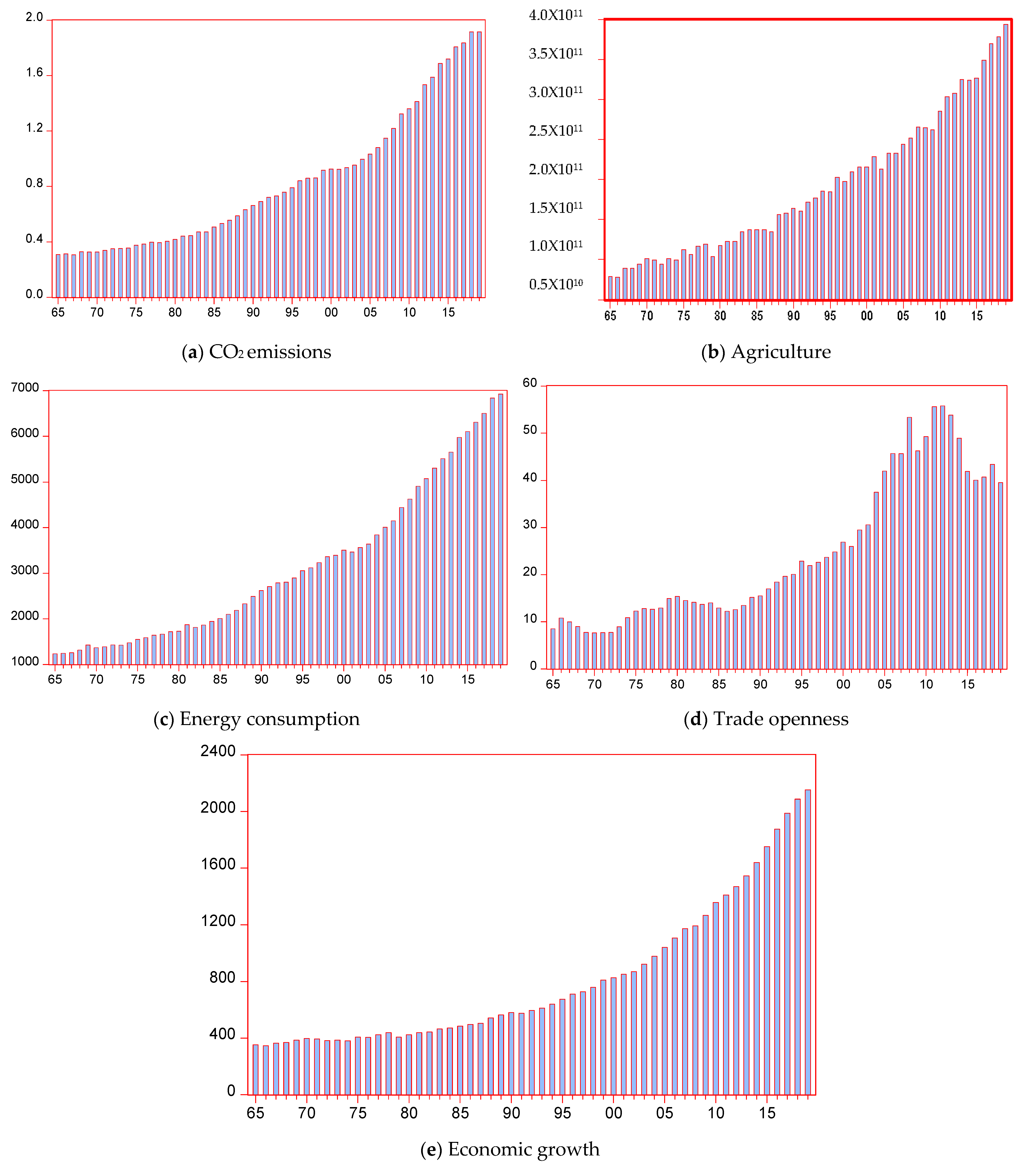
3.1. Data
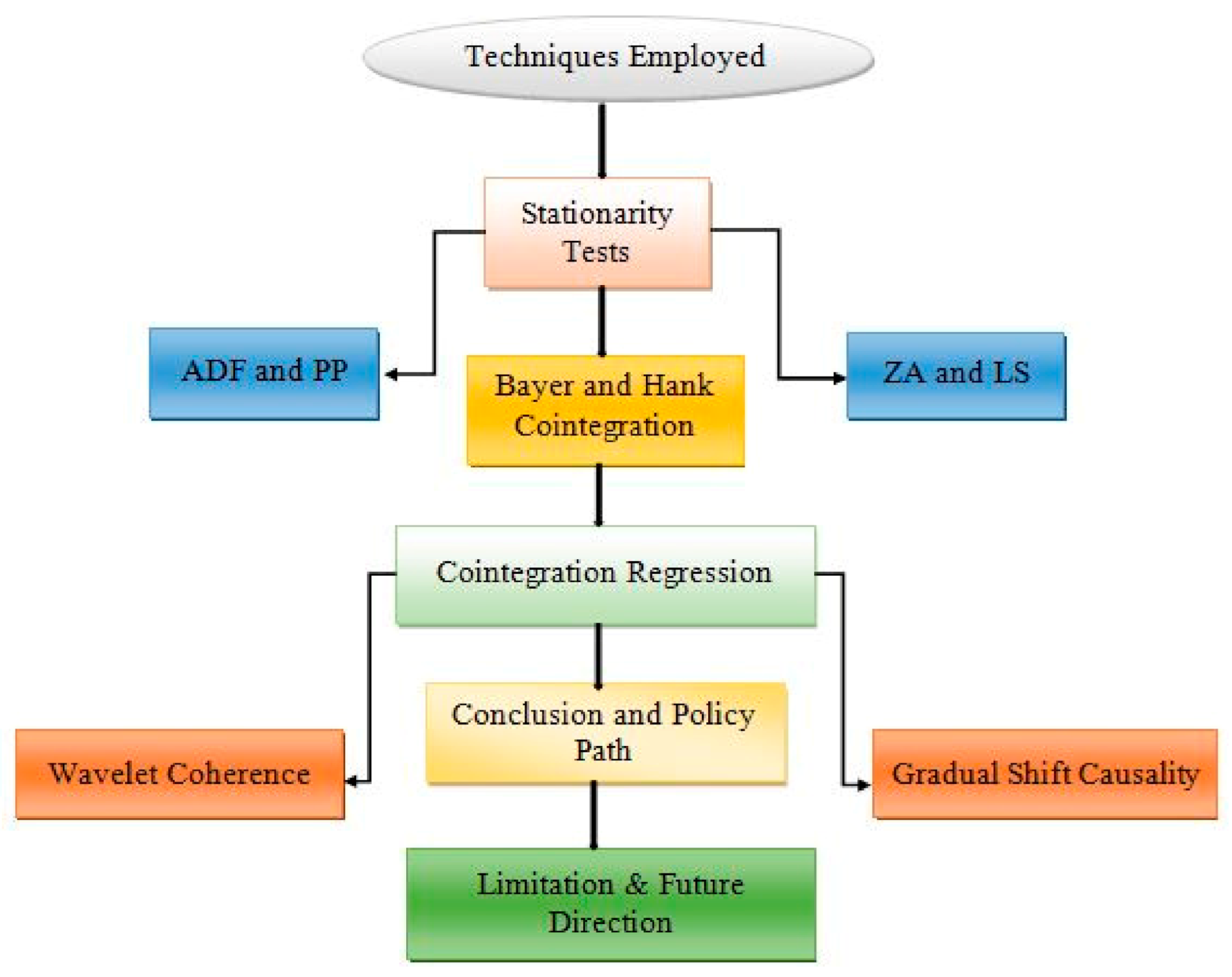
3.2. Methodology
3.2.1. Stationarity Tests
3.2.2. Cointegration Test
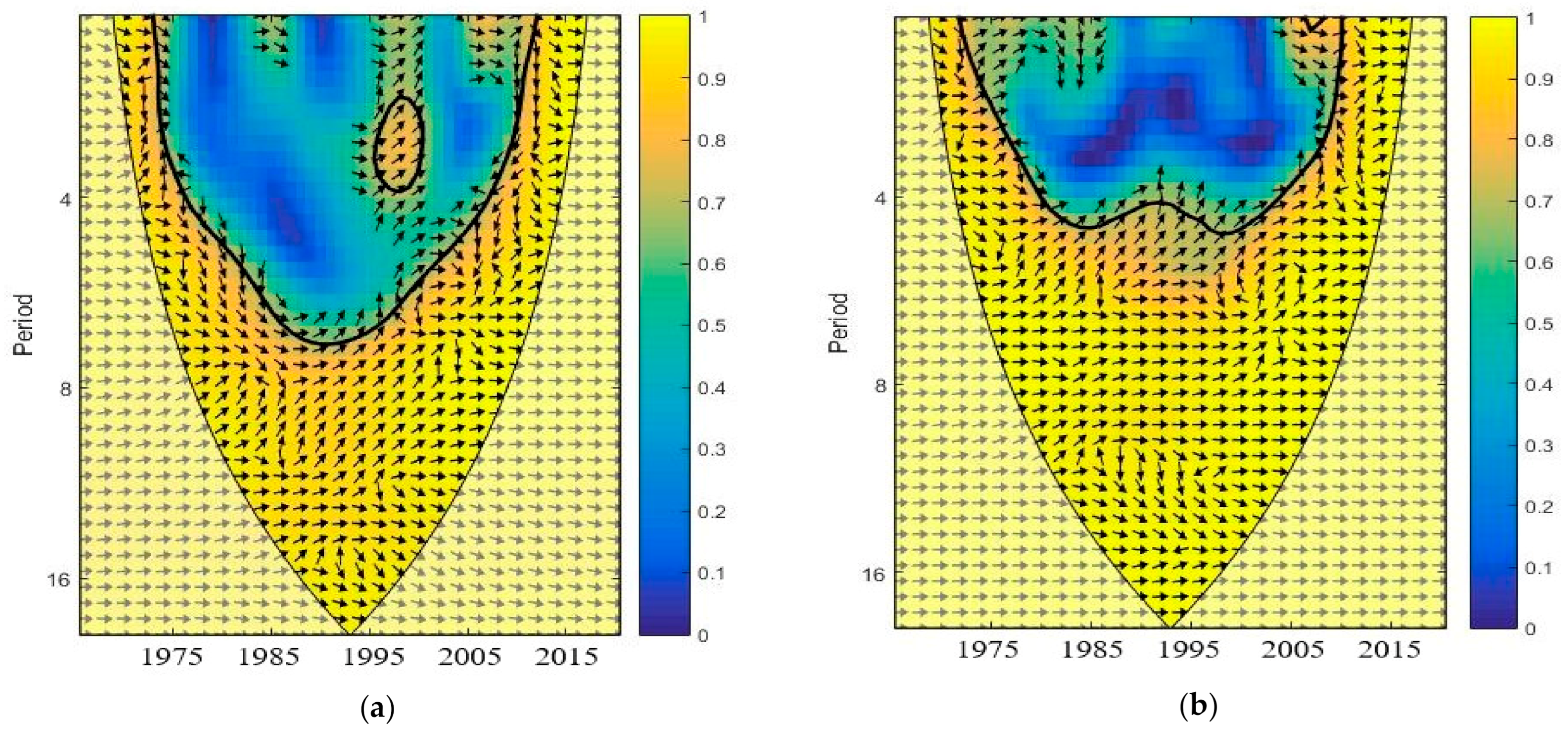
3.2.3. Wavelet Coherence Test
3.2.4. Gradual Shift Causality Test
4. Findings and Discussion
5. Conclusions and Policy Direction
Author Contributions
Funding
Institutional Review Board Statement
Informed Consent Statement
Data Availability Statement
Conflicts of Interest
References
- United Nations Economic and Social Commission for Asia and Pacific (UNESCAP). Asia and the Pacific SDG Progress Report 2019. 2019. Available online: https://www.unescap.org/publications/asia-and-pacific-sdg-progress-report-2019 (accessed on 19 February 2021).
- Shahbaz, M.; Sharma, R.; Sinha, A.; Jiao, Z. Analyzing nonlinear impact of economic growth drivers on CO2 emissions: Designingan SDG framework for India. Energy Policy 2021, 148, 111965. [Google Scholar] [CrossRef]
- United Nations. The Sustainable Development Goals Report 2019. 2019. Available online: https://unstats.un.org/sdgs/report/2019/ (accessed on 12 February 2021).
- Energy Information Administration (EIAU). International Energy Outlook. 2020; US Department of Energy. Available online: https://www.eia.gov (accessed on 4 March 2021).
- Asian Development Bank (ADB). Achieving Energy Security in Asia: Diversification, Integration and Policy Implications. 2019. Available online: https://www.adb.org/publications/achievingenergysecurityAsia (accessed on 23 February 2021).
- Kirikkaleli, D.; Adebayo, T.S. Do public-private partnerships in energy and renewable energy consumption matter for consumption-based carbon dioxide emissions in India? Environ. Sci. Pollut. Res. 2021, 1–14. [Google Scholar] [CrossRef]
- Khan, Z.; Hussain, M.; Shahbaz, M.; Yang, S.; Jiao, Z. Natural resource abundance, technological innovation, and human capital nexus with financial development: A case study of China. Resour. Policy 2020, 65, 101585. [Google Scholar] [CrossRef]
- Olanrewaju, V.O.; Adebayo, T.S.; Akinsola, G.D.; Odugbesan, J.A. Determinants of Environmental Degradation in Thailand: Empirical Evidence from ARDL and Wavelet Coherence Approaches. Pollution 2021, 7, 181–196. [Google Scholar]
- Shahbaz, M.; Raghutla, C.; Chittedi, K.R.; Jiao, Z.; Vo, X.V. The effect of renewable energy consumption on economic growth: Evidence from the renewable energy country attractive index. Energy 2020, 207, 118162. [Google Scholar] [CrossRef]
- Kalmaz, D.B.; Adebayo, T.S. Determinants of CO2 emissions: Empirical evidence from Egypt. Environ. Ecol. Stat. 2021, 1–24. [Google Scholar] [CrossRef]
- Rjoub, H.; Adebayo, T.S.; Awosusi, A.A.; Odugbesan, J.A.; Akinsola, G.D.; Wong, W.K. Sustainability of Energy-Induced Growth Nexus in Brazil: Do Carbon Emissions and Urbanization Matter? Sustainability 2021, 13, 4371. [Google Scholar]
- Magazzino, C.; Mele, M.; Schneider, N. The relationship between air pollution and COVID-19-related deaths: An application to three French cities. Appl. Energy 2020, 279, 115835. [Google Scholar] [CrossRef]
- Adebayo, T.S.; Kirikkaleli, D. Impact of renewable energy consumption, globalization, and technological innovation on environmental degradation in Japan: Application of wavelet tools. Environ. Dev. Sustain. 2021. [Google Scholar] [CrossRef]
- Zhang, L.; Li, Z.; Kirikkaleli, D.; Adebayo, T.S.; Adeshola, I.; Akinsola, G.D. Modeling CO2 emissions in Malaysia: An application of Maki cointegration and wavelet coherence tests. Environ. Sci. Pollut. Res. 2021, 1–15. [Google Scholar] [CrossRef]
- Ahmed, Z.; Adebayo, T.S.; Udemba, E.N.; Kirikkaleli, D. Determinants of consumption-based carbon emissions in Chile: An application of non-linear ARDL. Environ. Sci. Pollut. Res. 2021, 1–15. [Google Scholar] [CrossRef]
- Adams, S.; Adedoyin, F.; Olaniran, E.; Bekun, F.V. Energy consumption, economic policy uncertainty and carbon emissions; causality evidence from resource rich economies. Econ. Anal. Policy 2020, 68, 179–190. [Google Scholar] [CrossRef]
- Khan, Z.; Ali, S.; Dong, K.; Li, R.Y.M. How does fiscal decentralization affect CO2 emissions? The roles of institutions and human capital. Energy Econ. 2021, 94, 105060. [Google Scholar] [CrossRef]
- Adedoyin, F.F.; Gumede, M.I.; Bekun, F.V.; Etokakpan, M.U.; Balsalobre-Lorente, D. Modelling coal rent, economic growth and CO2 emissions: Does regulatory quality matter in BRICS economies? Sci. Total Environ. 2020, 710, 136284. [Google Scholar] [CrossRef]
- Adebayo, T.S. Testing the EKC hypothesis in Indonesia: Empirical evidence from the ARDL-based bounds and wavelet coherence approaches. Appl. Econ. 2021, 28, 1–23. [Google Scholar]
- Malik, M.Y.; Latif, K.; Khan, Z.; Butt, H.D.; Hussain, M.; Nadeem, M.A. Symmetric and asymmetric impact of oil price, FDI and economic growth on carbon emission in Pakistan: Evidence from ARDL and non-linear ARDL approach. Sci. Total Environ. 2020, 726, 138421. [Google Scholar] [CrossRef]
- Rjoub, H.; Odugbesan, J.A.; Adebayo, T.S.; Wong, W.K. Sustainability of the Moderating Role of Financial Development in the Determinants of Environmental Degradation: Evidence from Turkey. Sustainability 2021, 13, 1844. [Google Scholar] [CrossRef]
- Kirikkaleli, D.; Adebayo, T.S. Do renewable energy consumption and financial development matter for environmental sustainability? New global evidence. Sustain. Dev. 2020. [Google Scholar] [CrossRef]
- He, X.; Adebayo, T.S.; Kirikkaleli, D.; Umar, M. Analysis of Dual Adjustment Approach: Consumption-Based Carbon Emissions in Mexico. Sustain. Prod. Consum. 2021, 27, 947–957. [Google Scholar] [CrossRef]
- Cheikh, N.B.; Zaied, Y.B.; Chevallier, J. On the nonlinear relationship between energy use and CO2 emissions within an EKC framework: Evidence from panel smooth transition regression in the MENA region. Res. Int. Bus. Financ. 2021, 55, 101331. [Google Scholar] [CrossRef]
- Akinsola, G.D.; Adebayo, T.S. Investigating the causal linkage among economic growth, energy consumption and CO2 emissions in Thailand: An application of the wavelet coherence approach. Int. J. Renew. Energy Dev. 2021, 10, 17–26. [Google Scholar]
- Munir, Q.; Lean, H.H.; Smyth, R. CO2 emissions, energy consumption and economic growth in the ASEAN-5 countries: A cross-sectional dependence approach. Energy Econ. 2020, 85, 104571. [Google Scholar] [CrossRef]
- Siddique, H.M.A.; Majeed, D.M.T.; Ahmad, D.H.K. The impact of urbanization and energy consumption on CO2 emissions in South Asia. South Asian Stud. 2020, 31, 745–757. [Google Scholar]
- Adebayo, T.S. Revisiting the EKC hypothesis in an emerging market: Anapplication of ARDL-based bounds and wavelet coherence approaches. SN Appl. Sci. 2020, 2, 1–15. [Google Scholar] [CrossRef]
- Shahbaz, M.; Tiwari, A.K.; Nasir, M. The effects of financial development, economic growth, coal consumption and trade openness on CO2 emissions in South Africa. Energy Policy 2013, 61, 1452–1459. [Google Scholar] [CrossRef] [Green Version]
- Mahmood, H.; Maalel, N.; Zarrad, O. Trade openness and CO2 emissions: Evidence from Tunisia. Sustainability 2019, 11, 3295. [Google Scholar] [CrossRef] [Green Version]
- Hossain, M.S. Panel estimation for CO2 emissions, energy consumption, economic growth, trade openness and urbanization of newly industrialized countries. Energy Policy 2011, 39, 6991–6999. [Google Scholar] [CrossRef]
- Sun, H.; Attuquaye Clottey, S.; Geng, Y.; Fang, K.; Clifford Kofi Amissah, J. Trade openness and carbon emissions: Evidence from belt and road countries. Sustainability 2019, 11, 2682. [Google Scholar] [CrossRef] [Green Version]
- Dauda, L.; Long, X.; Mensah, C.N.; Salman, M.; Boamah, K.B.; Ampon-Wireko, S.; Dogbe, C.S.K. Innovation, trade openness and CO2 emissions in selected countries in Africa. J. Clean. Prod. 2021, 281, 125143. [Google Scholar] [CrossRef]
- Mutascu, M. A time-frequency analysis of trade openness and CO2 emissions in France. Energy Policy 2018, 115, 443–455. [Google Scholar] [CrossRef]
- Sebri, M.; Ben-Salha, O. On the causal dynamics between economic growth, renewable energy consumption, CO2 emissions and trade openness: Fresh evidence from BRICS countries. Renew. Sustain. Energy Rev. 2014, 39, 14–23. [Google Scholar] [CrossRef] [Green Version]
- Cetin, M.; Ecevit, E.; Yucel, A.G. The impact of economic growth, energy consumption, trade openness, and financial development on carbon emissions: Empirical evidence from Turkey. Environ. Sci. Pollut. Res. 2018, 25, 36589–36603. [Google Scholar] [CrossRef]
- Aydoğan, B.; Vardar, G. Evaluating the role of renewable energy, economic growth and agriculture on CO2 emission in E7 countries. Int. J. Sustain. Energy 2020, 39, 335–348. [Google Scholar] [CrossRef]
- Wang, J.; Dong, X.; Qiao, H.; Dong, K. Impact assessment of agriculture, energy and water on CO2 emissions in China: Untangling the differences between major and non-major grain-producing areas. Appl. Econ. 2020, 52, 6482–6497. [Google Scholar] [CrossRef]
- Doğan, N. The impact of agriculture on CO2 emissions in China. Panoeconomicus 2018, 66, 257–271. [Google Scholar] [CrossRef] [Green Version]
- Nwaka, I.D.; Nwogu, M.U.; Uma, K.E.; Ike, G.N. Agricultural production and CO2 emissions from two sources in the ECOWAS region: New insights from quantile regression and decomposition analysis. Sci. Total Environ. 2020, 748, 141329. [Google Scholar] [CrossRef]
- Ben Jebli, M.; Ben Youssef, S. Combustible renewables and waste consumption, agriculture, CO2 emissions and economic growth in Brazil. Carbon Manag. 2019, 10, 309–321. [Google Scholar] [CrossRef] [Green Version]
- Rehman, A.; Ozturk, I.; Zhang, D. The causal connection between CO2 emissions and agricultural productivity in Pakistan: Empirical evidence from an autoregressive distributed lag bounds testing approach. Appl. Sci. 2019, 9, 1692. [Google Scholar] [CrossRef] [Green Version]
- Waheed, R.; Chang, D.; Sarwar, S.; Chen, W. Forest, agriculture, renewable energy, and CO2 emission. J. Clean. Prod. 2018, 172, 4231–4238. [Google Scholar] [CrossRef]
- Jebli, M.B.; Youssef, S.B. The role of renewable energy and agriculture inr educing CO2 emissions: Evidence for North Africa countries. Ecol. Indic. 2017, 74, 295–301. [Google Scholar] [CrossRef] [Green Version]
- Adedoyin, F.F.; Nathaniel, S.; Adeleye, N. An investigation into the anthropogenic nexus among consumption of energy, tourism, and economic growth: Do economic policy uncertainties matter? Environ. Sci. Pollut. Res. 2021, 28, 2835–2847. [Google Scholar] [CrossRef]
- Ahmad, M.; Khan, Z.; Rahman, Z.U.; Khattak, S.I.; Khan, Z.U. Can innovation shocks determine CO2 emissions (CO2e) in the OECD economies? A new perspective. Econ. Innov. New Technol. 2021, 30, 89–109. [Google Scholar] [CrossRef]
- Zhang, J.; Zhang, Y. Tourism, economic growth, energy consumption, and CO2 emissionsin China. Tour. Econ. J. Clim. 2020, 12, 2679–2690. [Google Scholar]
- Khan, M.K.; Khan, M.I.; Rehan, M. The relationship between energy consumption, economic growth and carbon dioxide emissions in Pakistan. Financ. Innov. 2020, 6, 1–13. [Google Scholar] [CrossRef] [Green Version]
- Kuznets, S. Economic growth and income inequality. Am. Econ. Rev. 1955, 45, 1–28. [Google Scholar]
- Panayotou, T. Demystifying the environmental Kuznets curve: Turning a blackbox into a policy tool. Environ. Dev. Econ. 1997, 2, 465–484. [Google Scholar] [CrossRef] [Green Version]
- Grossman, G.M.; Krueger, A.B. Environmental Impacts of a North American Free Trade Agreement; (No.w3914); National Bureau of Economic Research: Cambridge, MA, USA, 1991. [Google Scholar]
- Kirikkaleli, D.; Adebayo, T.S.; Khan, Z.; Ali, S. Does globalization matter for ecological footprint in Turkey? Evidence from dual adjustment approach. Environ. Sci. Pollut. Res. 2020, 28, 1–9. [Google Scholar] [CrossRef]
- Kwiatkowski, D.; Phillips, P.C.; Schmidt, P.; Shin, Y. Testing the null hypothesis of stationarity against the alternative of a unit root: How sure are we that economic timeseries have a unit root? J. Econom. 1992, 54, 159–178. [Google Scholar] [CrossRef]
- Dickey, D.A.; Fuller, W.A. Likelihood ratio statistics for autoregressive time series with a unit root. Econom. J. Econom. Soc. 1981, 49, 1057–1072. [Google Scholar] [CrossRef]
- Phillips, P.C.; Perron, P. Testing for a unit root in time series regression. Biometrika 1988, 75, 335–346. [Google Scholar] [CrossRef]
- Odugbesan, J.A.; Rjoub, H. Relationship among economic growth, energy consumption, CO2 emission, and urbanization: Evidence from MINT countries. Sage Open 2020, 10, 2158244020914648. [Google Scholar] [CrossRef] [Green Version]
- Zivot, E.; Andrews, D.W.K. Further evidence on the great crash, the oil-price shock, and the unit-root hypothesis. J. Bus. Econ. Stat. 2002, 20, 25–44. [Google Scholar] [CrossRef]
- Lee, J.; Strazicich, M.C. Minimum Lagrange multiplier unit root test with two structural breaks. Rev. Econ. Stat. 2003, 85, 1082–1089. [Google Scholar] [CrossRef]
- Johansen, S. Estimation and hypothesis testing of cointegration vectors in Gaussian vector autoregressive models. Econom. J. Econom. Soc. 1991, 59, 1551–1580. [Google Scholar] [CrossRef]
- Engle, R.F.; Granger, C.W. Co-integration and error correction: Representation, estimation, and testing. Econom. J. Econom. Soc. 1987, 55, 251–276. [Google Scholar] [CrossRef]
- Banerjee, A.; Dolado, J.; Mestre, R. Error-correction mechanism tests for cointegration in a single-equation framework. J. Time Ser. Anal. 1998, 19, 267–283. [Google Scholar] [CrossRef] [Green Version]
- Boswijk, H.P. Efficient inference on cointegration parameters instructural error correction models. J. Econom. 1995, 69, 133–158. [Google Scholar] [CrossRef] [Green Version]
- Adebayo, T.S.; Kirikkaleli, D.; Adeshola, I.; Akinsola, G.D.; Oyebanji, M.; Osemeahon, O.S. Coal Consumption and Environmenta Sustainability in South Africa: The role of Financial Development and Globalization. Int. J. Renew. Energy Dev. 2021, 10, 527–536. [Google Scholar] [CrossRef]
- Bayer, C.; Hanck, C. Combining non-cointegration tests. J. Time Ser. Anal. 2013, 34, 83–95. [Google Scholar] [CrossRef]
- Torrence, C.; Webster, P.J. Interdecadal changes in the ENSO–monsoon system. J. Clim. 1999, 12, 2679–2690. [Google Scholar] [CrossRef] [Green Version]
- Grinsted, A.; Moore, J.C.; Jevrejeva, S. Application of the cross wavelet transform and wavelet coherence to geophysical time series. Nonlinear Process Geophys. 2004, 11, 561–566. [Google Scholar] [CrossRef]
- Torrence, C.; Compo, G.P. A Practical Guide to Wavelet Analysis; American Meteorological Society: Boston, MA, USA, 1998. [Google Scholar]
- Toda, H.Y.; Yamamoto, T. Statistical inference in vector autoregressions with possibly integrated processes. J. Econom. 1995, 66, 225–250. [Google Scholar] [CrossRef]
- Sims, C.A. Macroeconomics and reality. Econom. J. Econom. Soc. 1980, 48, 1–48. [Google Scholar] [CrossRef] [Green Version]
- Enders, W.; Jones, P. Grainprices, oil prices, and multiple smooth breaks in a VAR. Stud. Nonlinear Dyn. Econom. 2016, 20, 399–419. [Google Scholar]
- Nazlioglu, S.; Gormus, N.A.; Soytas, U. Oil prices and real estate investment trusts (REITs): Gradual-shift causality and volatility transmission analysis. Energy Econ. 2016, 60, 168–175. [Google Scholar] [CrossRef]
- Aguiar-Conraria, L.; Azevedo, N.; Soares, M.J. Using wavelets to decompose the time–frequency effects of monetary policy. Phys. A Stat. Mech. Appl. 2008, 387, 2863–2878. [Google Scholar] [CrossRef] [Green Version]
- Adebayo, T.S.; Odugbesan, J.A. Modeling CO2 emissions in South Africa: Empirical evidence from ARDL based bounds and wavelet coherence techniques. Environ. Sci. Pollut. Res. 2020, 28, 1–13. [Google Scholar] [CrossRef]
- Odugbesan, J.A.; Adebayo, T.S. The symmetrical and asymmetrical effects of foreign direct investment and financial development on carbon emission: Evidence from Nigeria. SN Appl. Sci. 2020, 2, 1–15. [Google Scholar] [CrossRef]
- Umar, M.; Ji, X.; Kirikkaleli, D.; Xu, Q. COP21 Roadmap: Do innovation, financial development, and transportation infrastructure matter for environmental sustainability in China? J. Environ. Manag. 2020, 271, 111026. [Google Scholar] [CrossRef]
- Panhwar, F. The Role of Nitrogen Fertiliser in Agriculture; Digital-Verlag Gmbh: Berlin, Germany, 2004. [Google Scholar]
- Adebayo, T.S.; Awosusi, A.A.; Kirikkaleli, D.; Akinsola, G.D.; Mwamba, M.N. Can CO2 Emissions and Energy Consumption Determine the Economic Performance of SouthKorea? A Time-Series Analysis. Environ. Sci. Pollut. Res. 2021, 1–15. [Google Scholar] [CrossRef]
- Oh, K.Y.; Bhuyan, M.I. Trade openness and CO2 emissions: Evidence of Bangladesh. Asian J. Atmos. Environ. 2018, 12, 30–36. [Google Scholar] [CrossRef]
- Saidi, K.; Mbarek, M.B. The impact of income, trade, urbanization, and financial development on CO2 emissions in 19 emerging economies. Environ. Sci. Pollut. Res. 2017, 24, 12748–12757. [Google Scholar] [CrossRef] [PubMed]


| CO2 Emissions and Economic Growth | ||||
|---|---|---|---|---|
| Author(s) | Period | Country(s) | Techniques | Conclusion |
| Zhang et al. [1] | 1970–2018 | Malaysia | Wavelet Coherence, ARDL, Gradual Shift | GDP ⇨ CO2 (+) GDP ⇨ CO2 |
| Adedoyin et al. [18] | 1995–2015 | Top ten earners | FMOLS, DOLS, D-H Causality | GDP ⇨ CO2 (−) CO2⇔GDP |
| Adebayo [19] | 1971–2016 | Indonesia | FMOLS, DOLS, ARDL | GDP ⇨ CO2 (+) |
| Ahmed et al. [15] | 1990–2018 | Chile | NARDL | GDP ⇨ CO2 |
| Kirikkaleli and Adebayo [6] | 1992–2015 | India | FMOLS, DOLS, Frequency Domain Causality | GDP ⇨ CO2 (+) GDP ⇨ CO2 |
| Adedoyin et al. [45] | 1990–2014 | BRICS | PMG-ARDL | GDP ⇨ CO2 (+) CO2⇨GDP |
| Adams et al. [16] | 1996–2017 | Countries with high geopolitical risk | PMG-ARDL, D-H Causality | GDP⇨CO2 (+) CO2⇔GDP |
| Ahmad et al. [46] | 1990–2014 | OECD economies | FMOLS | ⇨ CO2 (−) GDP ⇨ CO2 (+) |
| Khan et al. [17] | 1990–2018 | Seven OECD countries | PMG-ARDL, D-H Causality | GDP ⇨ CO2 (+) GDP ⇨ CO2 |
| Malik et al. [20] | 1971–2014 | Pakistan | Granger Causality | GDP ⇨ CO2 (+) CO2⇔GDP |
| Kirikkaleli and Adebayo [22] | 1980–2016 | Global Economy | FMOLS, DOLS, Frequency Domain Causality | GDP ⇨ CO2 (+) GDP ⇨ CO2 |
| Rjoub et al. [21] | 1960–2018 | Turkey | FMOLS, DOLS | GDP ⇨ CO2 (+) |
| CO2 Emissions and Energy Consumption | ||||
| He et al. [23] | 1990–2018 | Mexico | ARDL, FMOLS, DOLS, Frequency Domain Causality | EC ⇨ CO2 (+) EC ⇨ CO2 |
| Zhang and Zhang [47] | 2000–2017 | 30 Chinese provinces | VECM | EC ⇨ CO2 |
| Adebayo [28] | 1970–2016 | Mexico | ARDL, FMOLS, DOLS, Wavelet Coherence | EC ⇨ CO2 (+) EC ⇨ CO2 |
| Olanrewaju et al. [8] | 1970–2016 | Thailand | ARDL, FMOLS, DOLS, Wavelet Coherence | EC ⇨ CO2 (+) EC ⇨ CO2 |
| Siddique et al. [27] | 1983–2013 | South Asia | Panel Granger Causality | EC ⇨ CO2 |
| Akinsola and Adebayo [25] | 1970–2016 | Thailand | Wavelet Coherence, Granger Causality | EC ⇨ CO2 (+) EC ⇨ CO2 |
| Cheikh et al. [36] | 1980–2015 | 12 MENA countries | PSTR | EC⇨CO2 |
| Khan et al. [48] | 1965–2015 | Pakistan | ARDL | EC ⇨ CO2 (+) |
| Odugbesan and Rjoub [11] | 1993–2017 | MINT | ARDL, Granger Causality | EC ⇨ CO2 |
| Munir et al. [26] | 1980–2016 | ASEAN-5 | FMOLS, Granger Causality | EC ⇨ CO2 |
| CO2 Emissions and Agriculture | ||||
| Wang et al. [38] | 2004–2017 | China | GMM | AGRIC ⇨ CO2 (+) |
| Aydoğan and Vardar [37] | 1990–2014 | E7 countries | OLS, DOLS, FMOLS | AGRIC ⇨ CO2 (+) |
| Jebli and Youssef [44] | 1980–2011 | North Africa countries | Granger Causality | AGRIC ⇨ CO2 (–) AGRIC⇔CO2 |
| Doğan 38] | 1971–2010 | China | ARDL, FMOLS, DOLS, CCR | AGRIC ⇨CO2 ((+) AGRIC⇔CO2 |
| Nwaka et al. [40] | 1990–2015 | West African economies | Panel Techniques | AGRIC ⇨ CO2 (+) |
| Rehman et al. [42] | 1987–2017 | Pakistan | ARDL | AGRIC ⇨ CO2 (+) |
| Ben Jebli and Ben Youssef [41] | 1980–2013. | Brazil | ARDL | AGRIC ⇨ CO2 (+) |
| CO2 Emissions and Trade Openness | ||||
| Shahbaz et al. [29] | 1965–2008 | South Africa | ARDL | TO ⇨ CO2 (–) |
| Mutascu [34] | 1960–2013 | France | Wavelet Coherence | TO CO2 |
| Sebri and Ben-Salha [35] | 1971–2010 | BRICS | VECM | TO ⇨ CO2 (+) |
| Mahmood et al. [30] | 1971–2011 | Tunisia | ARDL | TO ⇨ CO2 (+) |
| Hossain [31] | 1971–2007 | Newly industrialized countries | Granger Causality | TO CO2 |
| Dauda et al. [33] | 1990–2016 | 9 African nations | GMM | Mixed Findings |
| Sun et al. [32] | 1991–2014 | Several Nations | VECM | Mixed Findings |
| Cetin et al. [36] | 1960–2013 | Turkey | VECM | TO ⇨ CO2 |
| Variable | Description | Units | Sources |
|---|---|---|---|
| Economic Growth | GDP per capita in constant USD, 2010 | WDI | |
| Trade Openness | Trade % of GDP | WDI | |
| AGRIC | Agriculture | Agriculture, fishing, and forestry, value-added | WDI |
| CO2 | CO2 Emissions | Per capita emissions | BP |
| Energy Use | Energy consumption per capita (kWh) | BP |
| CO2 | EC | GDP | TO | AGRIC | |
|---|---|---|---|---|---|
| Mean | 0.8267 | 3134.5 | 815.5158 | 24.578 | 1.91 × 10¹¹ |
| Median | 0.7216 | 2790.4 | 595.0135 | 18.433 | 1.71 × 10¹¹ |
| Maximum | 1.9157 | 6923.9 | 2151.726 | 55.793 | 3.94 × 10¹¹ |
| Minimum | 0.3070 | 1234.19 | 345.42 | 7.6617 | 7.75 × 10¹⁰ |
| Std. Dev. | 0.4876 | 1685.5 | 506.44 | 15.306 | 8.78 × 10¹⁰ |
| Skewness | 0.8500 | 0.7644 | 1.1901 | 0.7157 | 0.654237 |
| Kurtosis | 2.5867 | 2.4315 | 3.3230 | 2.0704 | 2.363121 |
| Jarque–Bera | 7.0152 | 6.0972 | 13.223 | 6.6758 | 4.853106 |
| Probability | 0.0299 | 0.0474 | 0.0013 | 0.0355 | 0.088341 |
| Observations | 55 | 55 | 55 | 55 | 55 |
| ADF Unit Root Test | |||
|---|---|---|---|
| At Level I (0) | First Difference I (1) | Decision | |
| T and I | T and I | ||
| GDP | −0.9012 | −6.4815 * | I (1) |
| CO2 | −2.6626 | −7.3821 * | I (1) |
| EC | −2.5039 | −8.4014 * | I (1) |
| TO | −1.3876 | −5.7691 * | I (1) |
| AGRIC | −5.6106 * | −7.8427 * | I (0),I (0) |
| PP Unit Root Test | |||
| GDP | −0.7133 | −9.8978 * | I (1) |
| CO2 | −2.6671 | −7.4401 * | I (1) |
| EC | −2.4969 | −8.3571 * | I (1) |
| TO | −1.8396 | −5.8967 * | I (0),I (1) |
| AGRIC | −5.7122 * | −15.620 * | I (0) |
| At Level I (0) | First Difference I (1) | Decision | |||
|---|---|---|---|---|---|
| ZA unit root test | |||||
| Variables | T and I | Break-Date | T and I | Break-Date | |
| GDP | −2.4908 | 1979 | −6.2685 ** | 1985 | I (1) |
| CO2 | −2.9007 | 2000 | −8.2378 * | 1991 | I (1) |
| EC | −3.1018 | 1978 | −8.8344 * | 1991 | I (1) |
| TO | −3.8386 | 2004 | −6.9854 * | 1976 | I (1) |
| AGRIC | −7.0528 * | 1979 | −6.9761 * | 2002 | I (0), I (1) |
| LSunit root test | |||||
| GDP | −5.2403 | 1980 and 1997 | −8.8362 | 1977 and 1989 | I (1) |
| CO2 | −4.6148 | 1984 and 1998 | −5.8828 *** | 1995 and 2004 | I (1) |
| EC | −4.8448 | 1992 and 2001 | −8.3239 | 1975 and 1978 | I (1) |
| TO | −5.6633 | 1991 and 2008 | −6.2901 ** | 1987 and 2001 | I (1) |
| AGRIC | −6.0759 ** | 1990 and 2002 | −7.9906 * | 1994 and 2009 | I (0), I (1) |
| Model | Fisher Statistics | Fisher Statistics | Cointegration Decision |
|---|---|---|---|
| CO2 = f(GDP, EC, TO, AGRIC) | EG-JOH | EG-JOH-BAN-BOS | |
| 27.978 ** | 36.593 ** | Yes | |
| CV | CV | ||
| 5% | 10.576 | 20.143 |
| Frequency | Significance of the Correlation | Strength of the Correlation |
|---|---|---|
| High | CO2⇔GDP (Yes) | Weak |
| Medium | CO2⇔GDP (Yes) | Strong |
| Low | CO2⇔GDP (Yes) | Strong |
| High | CO2⇔EC (Yes) | Weak |
| Medium | CO2⇔EC (Yes) | Strong |
| Low | CO2⇔EC (Yes) | Strong |
| High | CO2⇔TO (Yes) | Weak |
| Medium | CO2⇔TO (Yes) | Weak |
| Low | CO2⇔TO (No) | Null |
| High | CO2⇔AGRIC (Yes) | Weak |
| Medium | CO2⇔AGRIC (Yes) | Strong |
| Low | CO2⇔AGRIC (Yes) | Strong |
| Causality Path | WaldStat | No. of Fourier | p-Value | Decision |
|---|---|---|---|---|
| GDP → CO2 | 4.3821 | 3 | 0.7348 | Do not Reject Ho |
| CO2→ GDP | 14.031 *** | 3 | 0.0505 | Reject Ho |
| EC → CO2 | 27.609 * | 3 | 0.0002 | Reject Ho |
| CO2 → EC | 6.8497 | 3 | 0.4446 | Do not Reject Ho |
| AGRIC → CO2 | 25.7567 * | 2 | 0.0000 | Reject Ho |
| CO2 → AGRIC | 27.131 * | 2 | 0.0000 | Reject Ho |
| TO → CO2 | 10.050 | 2 | 0.1857 | Do not Reject Ho |
| CO2 → TO | 5.4607 | 2 | 0.6039 | Do not Reject Ho |
Publisher’s Note: MDPI stays neutral with regard to jurisdictional claims in published maps and institutional affiliations. |
© 2021 by the authors. Licensee MDPI, Basel, Switzerland. This article is an open access article distributed under the terms and conditions of the Creative Commons Attribution (CC BY) license (https://creativecommons.org/licenses/by/4.0/).
Share and Cite
Orhan, A.; Adebayo, T.S.; Genç, S.Y.; Kirikkaleli, D. Investigating the Linkage between Economic Growth and Environmental Sustainability in India: Do Agriculture and Trade Openness Matter? Sustainability 2021, 13, 4753. https://0-doi-org.brum.beds.ac.uk/10.3390/su13094753
Orhan A, Adebayo TS, Genç SY, Kirikkaleli D. Investigating the Linkage between Economic Growth and Environmental Sustainability in India: Do Agriculture and Trade Openness Matter? Sustainability. 2021; 13(9):4753. https://0-doi-org.brum.beds.ac.uk/10.3390/su13094753
Chicago/Turabian StyleOrhan, Ayhan, Tomiwa Sunday Adebayo, Sema Yılmaz Genç, and Dervis Kirikkaleli. 2021. "Investigating the Linkage between Economic Growth and Environmental Sustainability in India: Do Agriculture and Trade Openness Matter?" Sustainability 13, no. 9: 4753. https://0-doi-org.brum.beds.ac.uk/10.3390/su13094753