To What Extent May Transit Stop Spacing Be Increased before Driving Away Riders? Referring to Evidence of the 2017 NHTS in the United States

Abstract

With the emergence of ride-sourcing and ride-splitting services, more options are available to support shifts away from transit, where maintaining transit ridership increases requirements for transit service quality, so as to promote high-capacity and sustainable transport systems. In this endeavor, proper transit stop spacing is critical for both service accessibility and in-vehicle trip efficiency, as well as operation cost. This research explores acceptable stop spacing for three kinds of transit services from the perspective of travel behavior, drawing on the 2017 National Household Travel Survey in the United States. A stochastic frontier model is developed to infer passengers’ unobservable vertex of acceptable transit access times on the basis of observed walk time, which can be converted to the tolerance with respect to stop spacing with the average walking speed. Significant explanatory variables on the vertex of acceptable transit stop spacing are further identified with their quantified impacts, including household density, household income, wait time, trip distance, transfer, and maintenance purpose, while the inefficiency variance is significantly related to traveler age, wait time, secondary walk time, and trip frequency. Recommended response strategies follow. Findings from this study provide insights, guidelines, and implementation plans for different transit agencies when considering stop spacing redesign, to strengthen transit service appeal and to promote cooperative and sustainable multi-modal urban transport systems.

1. Introduction

With urbanization and motorization, population is increasingly concentrating in metropolitan areas, leading to serious congestion, undue trip delays, tremendous economy losses, inequality in employment and education, and heavy emissions [1]. This poses a great threat to society sustainability. Public transport is a well-accepted remedy to such challenges, which enhances road utility by carrying mass passengers at one time at subsidized prices. However, the world has witnessed appreciable losses in transit ridership since 2010 [2], especially against the rapid development of ride-sourcing and ride-splitting to provide travelers an alternative to transit with flexible ad-convenient services at a competitive cost [3,4]. Given the transit advantages of serving dense passengers [5] over medium or long distances and promoting social equality [6], it is necessary to keep transit attractive and retain its ridership for well-organized and sustainable transport systems, where stop spacing is a fundamental point.

This research draws on the 2017 National Household Travel Survey (NHTS) in the United States, to explore passengers’ tolerance with respect to transit stop spacing at the trip level. Contribution of this study can be summarized as below.

(a)

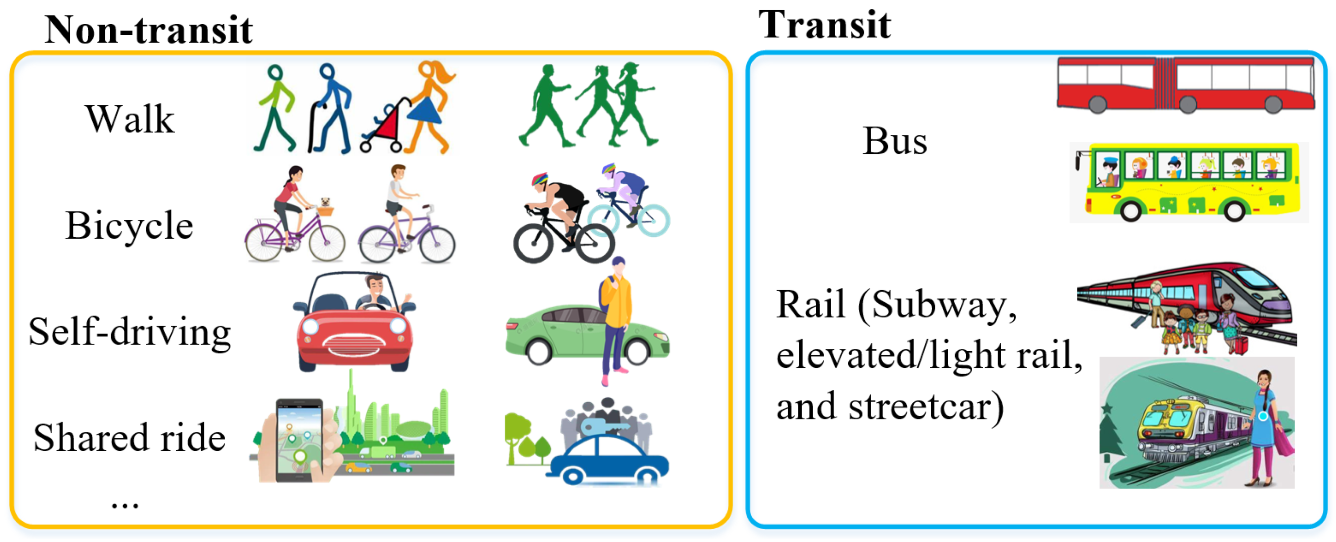
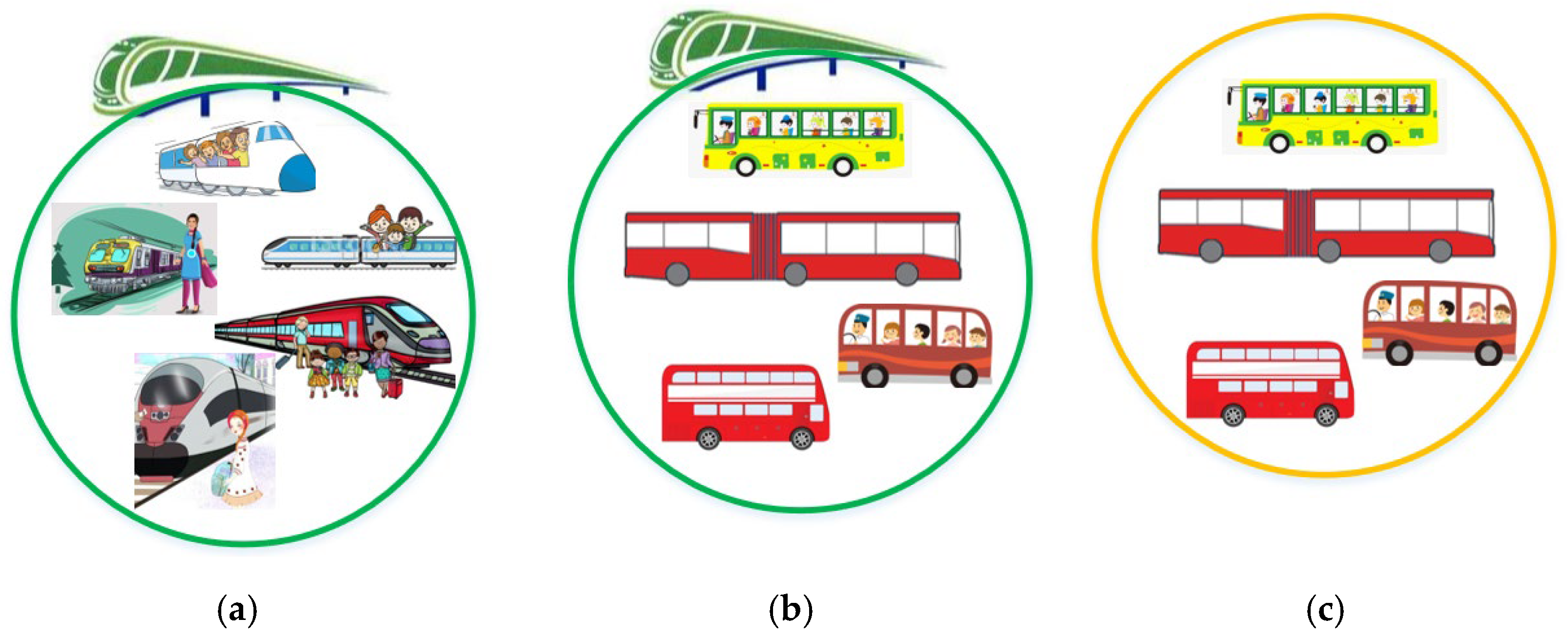
Referring to the 2017 NHTS in the United States, acceptable stop spacing is analyzed separately for rail and bus services, with the latter categorized to be those in areas with and without heavy rail.

(b)

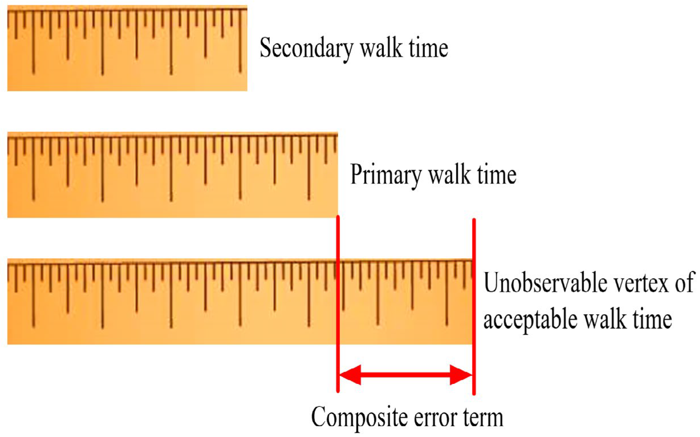
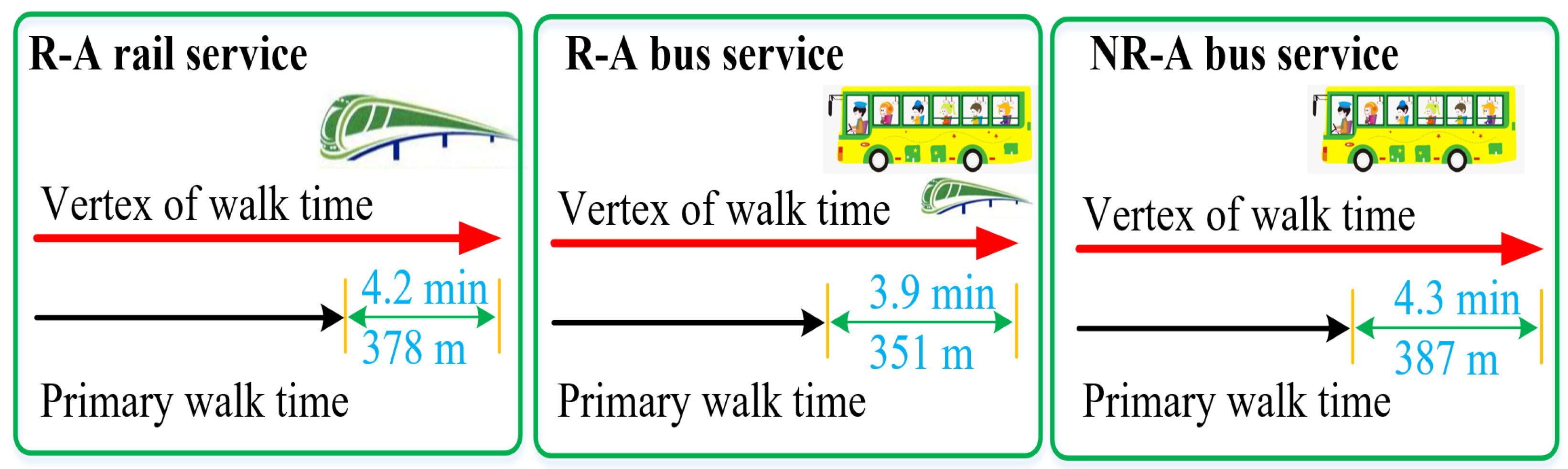
A stochastic frontier model (SFM) is proposed to infer the vertex of transit stop walk time by integrating multi-dimensional factors of passenger socio-economics and trip attributes with a deterministic frontier part and the stochastic error, where the former indicates the maximum stop spacing that is tolerable, to reduce transit service costs and delays without disappointing passengers.

(c)

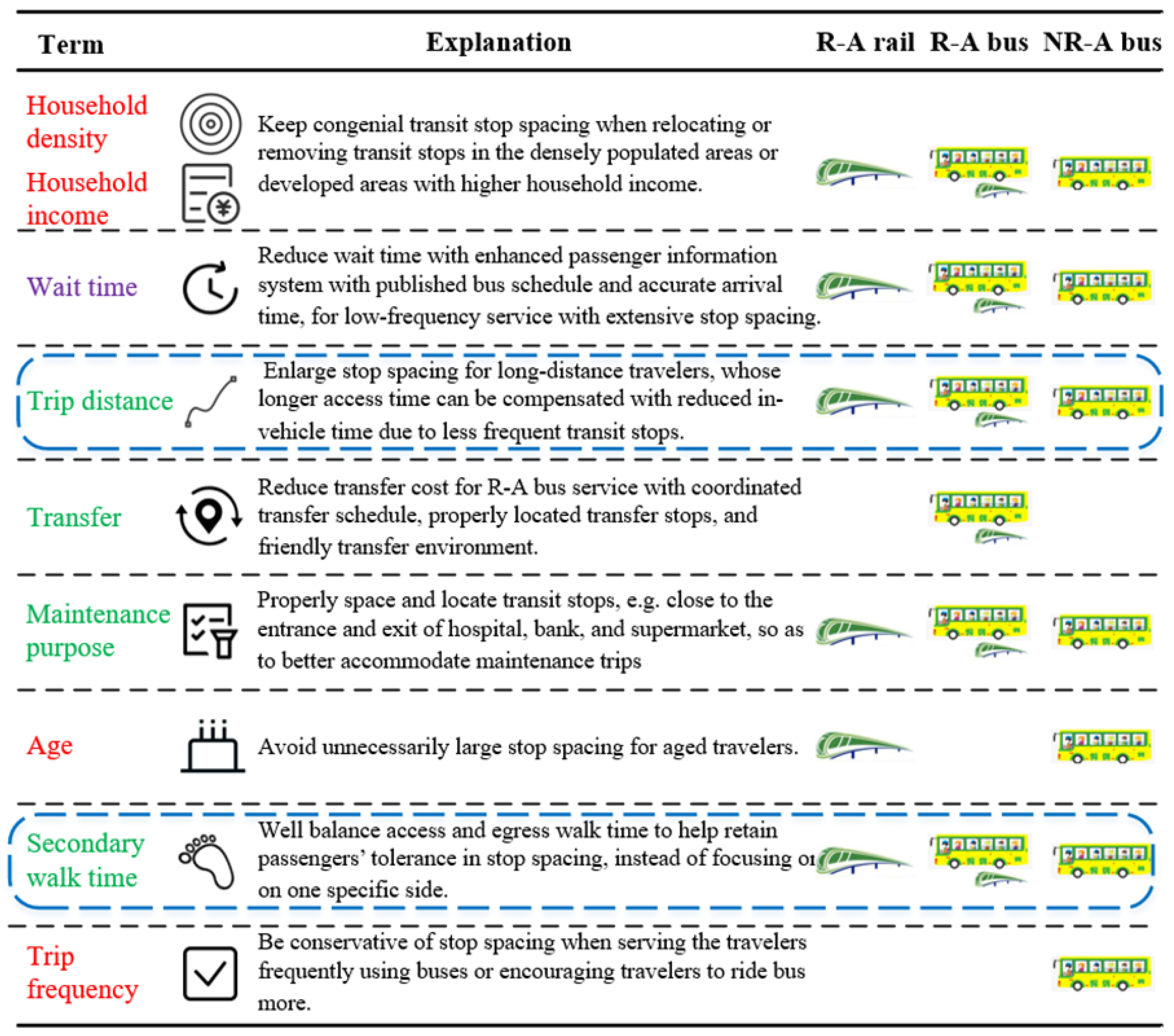
Results are discussed to reveal the statistical factors on the stop spacing vertex, based on which response strategies are developed for each type of transit service, so as to proactively suit transit stop spacing to specific conditions and thereby improve transit service quality and appeal, promoting transport sustainability.

The rest of the paper is organized as follows. Section 2 reviews the relevant literature, Section 3 introduces the data source and processing of the 2017 NHTS in the United States. Section 4 describes SFM to estimate the acceptable transit stop spacing based on the observed walk time, with explanatory variables of passenger socio-demographics and trip attributes. Section 5 presents the results and discusses the suggested policies in transit stop spacing. Finally, brief conclusions are drawn, and future research directions are given in Section 6.

2. Literature Review

Stop spacing requires judicious balance between service accessibility and operation efficiency [7], two dominating factors on transit choice [8] to influence transport system structure and sustainability. Larger stop spacing reduces transit accessibility, but cuts down operation delay with less frequent pulling in and out, thereby reducing operation costs. In contrast, small stop spacing contributes to congenial accessibility, but reduces transit operation efficiency with continuous deceleration and acceleration as well as dwelling at stops, in addition to energy consumption and pollutant emissions. For example, the Maryland Transport Association [9] provided empirical support that the bus running speed was nearly 18 km/h with a stop spacing of no more than 150 m, only comparable to that of bicycling. London stated that 300–1000 m bus stop spacing corresponded to an average operation speed between 12 and 25 km/h, respectively [10], though exclusive bus lanes may enhance operation efficiency [11]. Similar conclusions have been established for rail services, where reducing station spacing from 1600 to 400 m cut down operation speed by 30% under the same passenger distribution [12].

Empirically, there is a wide gap of agency standards on transit stop spacing. Transit capacity and quality of service manual recommended stop spacing of air distance 400 and 800 m for bus and rail, respectively [13]. Guidelines on bus stop spacing range from 200 to 600 m around the world in urban areas [14]. Local buses generally stop every 400 m in Australia and most parts of Europe, and as frequently as every 200 m in the United States [15]. It has been stated that nearly all bus inter-stop distance in Western Europe far exceeded that in the United States, e.g., 3–4 stops vs. 7–10 stops per mile, respectively [16]. Though many agencies in the United States have reexamined the possibility of enlarging bus stop spacing, the newly adopted wider spacing standard was still conservative and significantly smaller than that of European bus systems [9]. Urban rail station spacing also varies significantly, against its impact on service accessibility and operation cost [17]. For example, Canada guidelines on walk distance to light rail station ranged between 300 and 900 m, and the Toronto Transit Commission recommended station spacing as small as 300 m [18]. Statistical analysis compared the changes in the station spacing of typical cities, e.g., Chicago and Washington, and found that average station spacing has decreased significantly in recent decades [19]. Therefore, ideal transit stop spacing is advocated.

Theoretically, there is extensive literature documenting the factors of stop spacing. At the city level, Nes conducted a series of simulations and found that the optimal bus stop spacing in the small and large cities was 600 and 800 m, respectively, against the factors of travel time, operator costs, and patronage [20]. At the zonal level, bus stop spacing was basically dependent on land use density. For example, Greenville in the United States recommended bus stop spacing of 200 m for city centers and main corridors with high density, in comparison to 400 m in suburban areas, so as to secure service accessibility [21]. Similar conclusions have been reached for rail station spacing, being 500 m or less in dense areas and 1.6 km or more in suburban areas [22,23]. Though such design reduces total passenger access cost, its deficiency can be threefold: (a) in-vehicle delay is unavoidably increased in dense areas with a high loading factor, and the social optimum is not well considered as captive riders concentrate more in transit-underserved areas [24,25]; (b) such aggregate analysis can be criticized as inaccurate, as it fails to include a situational context and to adjust stop spacing proactively [26]; (c) it fails to investigate the impact of stop spacing from both access and egress ends, thereby leading to incomplete and biased conclusions.

Recently, delicate research has been implemented to account for the effect of passenger characteristics and service quality on transit stop spacing. With respect to passenger socio-economics, Kim et al. [27] conducted a questionnaire to obtain passengers’ socio-demographics and transit use information in various city types, including the factors of gender, age, employment status, income, car ownership, transit use frequency, trip purpose, and access mode [28]. With cross-sectional statistics and adaptive neuro-fuzzy inference model, it was found that age and income significantly influenced the maximum acceptable walk time to transit stops. Further, it was demonstrated that women tended to walk a longer distance than men to access transit service [29,30]. Service quality also influenced acceptable stop spacing, where O’Connor [31] employed the 85th percentile walk distance to find that the acceptable spacing of high quality bus service (e.g., BRT) could be enlarged to 1400 m, times of that of regular bus service. Further, McIntosh et al. [32] and Jiang et al. [33] found that access amenity extended bus stop spacing to between 800 and 1600 m with ordinary regression, while stated preferences showed that a friendly walk environment could extend rail station spacing by 1.6 to 1.77 times [34].

Passengers’ trip attributes also have a significant effect on stop spacing by mediating travel behavior [35,36]. For example, long-distance travelers prefer larger stop spacing, so as to reduce in-vehicle delay [37]. However, to what extent trip distance influences stop spacing has not been well explored. In addition, passengers’ daily trip frequency may also cause radical changes in the vertex (i.e., upper bound) of acceptable transit spacing due to the accumulated trip delay [38] from accessing to and egressing from transit stops. Moreover, passengers tolerating a bus headway 10 min longer than average were found to accept longer walk distances by 200 to 500 m, with a stated choice experiment [39]. Considering that stated preferences could be quite different from actual passenger behavior, removing their inconsistency calls for an appropriate method to accurately understand passengers’ acceptable transit stop spacing.

To address the above gap, this research employs passenger stop walk time, the major feeder mode to or from transit stops, for an exploration of their vertex of transit stop walk time, which can be converted to passengers’ acceptable stop spacing with average walking speed. Given that passengers’ actual access time is governed by and always no larger than the unobservable walk time vertex, the latter is inferred from the former with a stochastic frontier model (SFM) at trip level [40,41], based on the 2017 National Household Travel Survey (NHTS) in the United States [42]. SFM integrates passenger socio-economics and trip attributes to identify the factors on the vertex of acceptable stop walk time in two parts [43]. The first part is a deterministic frontier function for the vertex of passenger tolerance with respect to stop walk time against socio-demographics and trip attributes. The second is a composite error term, capturing the factors that hinder passengers from achieving the frontier under uncertainty [44].

3. Data Description

3.1. Data Structure

This research employs the data from the household-based 2017 NHTS by the Department of Transportation in the United States [42]. It collected information of all trips from the members that were no younger than 5 years old of selected households on a randomly assigned survey day. It used an address-based sample frame, where household recruitment and person-retrieval survey were completed in the first and second stage, respectively. The weighted person-level response rate was 15.6% in the dataset.

Figure 1 illustrates the definition of transit trips from the 2017 NHTS, referring to trips where (1) the trip mode is a bus or (2) the trip mode is rail, such as subway, elevated/light rail, and streetcar. Transit trip information from the 2017 NHTS in the United States includes trip ID, access mode and time, wait time, transfer count, egress time and mode, trip distance, trip time, trip purpose, and area type (being urban or suburban). A total of 9606 transit trips were recorded in urban areas, while much fewer were recorded in suburban areas. Thus, we focus on urban transit trips here.

Table 1. Comparison of the trips in the urban areas with and without heavy rail.

Areas	With Heavy Rail	Without Heavy Rail
Total trips	146,130	777,442
Transit trips	3729	3819
Bus trips	1692	3329
Rail trips	2037	490
Transit share	2.6%	0.5%

compares urban transit trips in the areas with and without heavy rail, with a transit share of 2.6% and 0.5%, respectively. Given such a significant difference in transit share, areas are accordingly categorized with respect to the absence of heavy rail. Further, rail and bus services are also distinguished due to their different service characteristics [13]. Thus, urban transit trips are divided into four groups, i.e., rail and bus trips in the areas with and without heavy rail. Moreover, due to the small count of rail trips in the areas without heavy rail, rail trips in the no-heavy-rail areas (NR-A) are excluded from the following analysis. Figure 2 shows the three types of transit service explored in the research: (1) rail service in the heavy rail areas (R-A); (2) bus service in R-A; and (3) bus service in NR-A.

Moreover, the following data is excluded: (1) trips with incomplete information, such as unstated gender, age, trip mode, and time to access to or egress from transit service, (2) trips by travelers younger than 16 years old, who are not capable of independently choosing a transport mode, and (3) inter-urban trips with travelers out of town on the survey day or trip distance longer than 15 km.

Table 2. Comparison of the selected and all transit trips.

Transit Trips	Parameters	R-A Rail Service	Bus Service
			R-A	NR-A
Selected data	Female (%)	53.6	58.3	49
	Worker (%)	16.8	46.5	51.5
	Driver (%)	29.1	52.6	57.4
	Average walk time (min)	8.0	9.4	7.6
	Average transfer times per trip	0.4	0.5	0.6
Whole dataset	Female (%)	50.1	55.3	48.7
	Worker (%)	13.7	34	38
	Driver (%)	18.9	42.1	44.3
	Average stop walk time (min)	10.5	10.4	9.1
	Average transfer times per trip	0.4	0.5	0.5

summarizes the statistics of the selected data and those from the whole dataset. The selected data slightly overrepresents females, workers, and drivers of both rail and bus trips, while the average stop walk time is underestimated. Such bias is reasonable because suburban and inter-urban trips are excluded from the selected data, where males account for a larger proportion, and 5–16-year-old passengers’ trips are also removed, as such passengers are not workers or drivers. Additionally, the average bus walk time from the selected data is appreciably larger than the suggested value from the existing research on transit in the United States, i.e., 5 min [13,45], indicating the potential and value of digging with regard to the acceptable stop spacing.

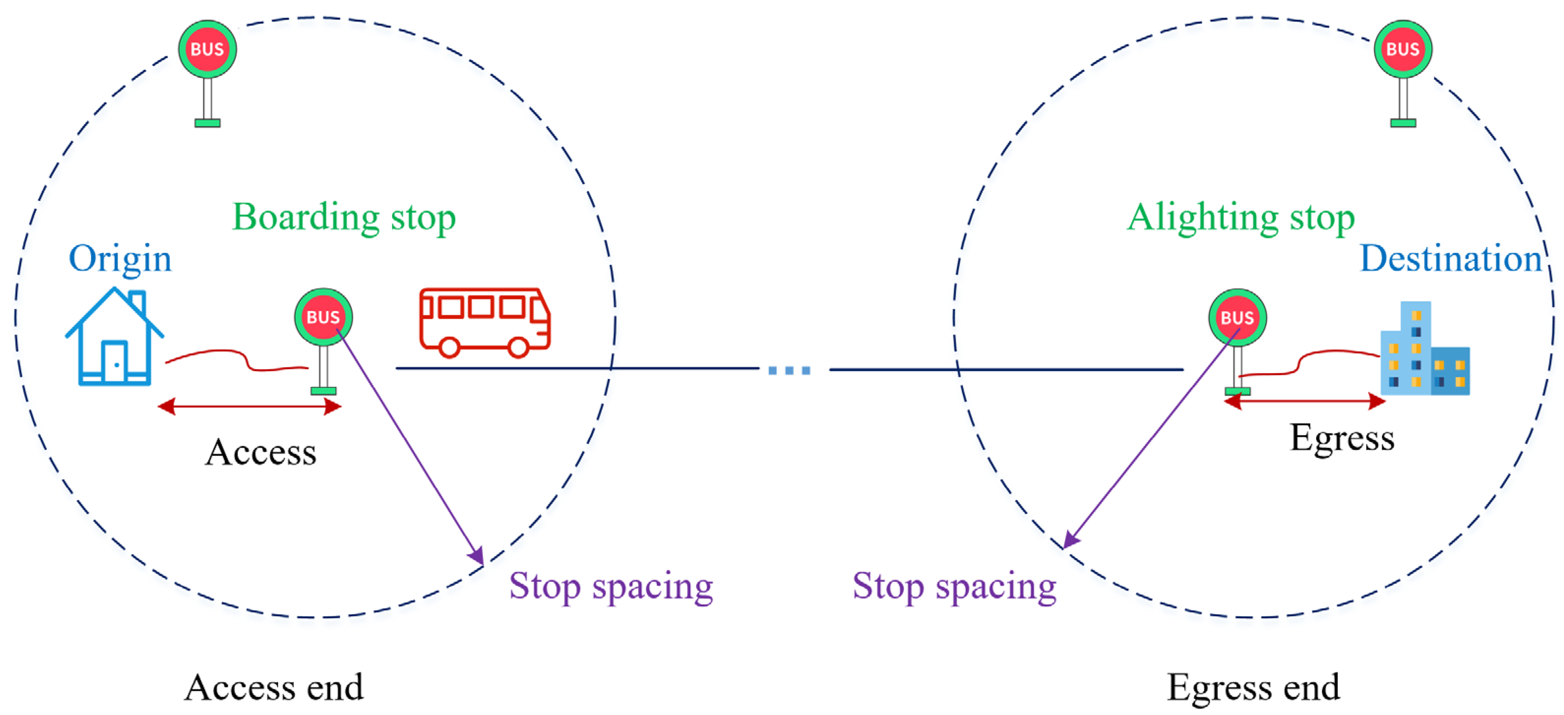
3.2. Representation of Stop Spacing

Figure 3 shows the influence of transit stop spacing on the two ends of transit trips. The first end is to access the boarding stop from the trip origin, and the second end is to egress from the alighting stop to the destination. The access or egress distance can be inferred from the stop access or egress time in the 2017 NHTS multiplied by the average speed of access/egress mode. Figure 4 demonstrates that walking mode accounts for the largest share, being more than 80% for both access to or egress from rail and bus stops in both R-A and NR-A. Thus, the following analysis focuses on stop walk time, which can be transformed to stop spacing with the average walking speed.

The larger value between the walk access time and the walk egress time, i.e., the primary walk time, is employed to represent passengers’ observable acceptance of stop spacing, while the smaller value is defined as secondary walk time to be a predictor variable of the vertex of acceptable stop walk time. Figure 5 shows the difference of primary and secondary walk time, as well as the unobservable vertex of walk time. Primary walk time is always no larger than the unobservable vertex of acceptable stop walk time, where the latter can be inferred from the former with SFM developed in the following section.

4. Methods

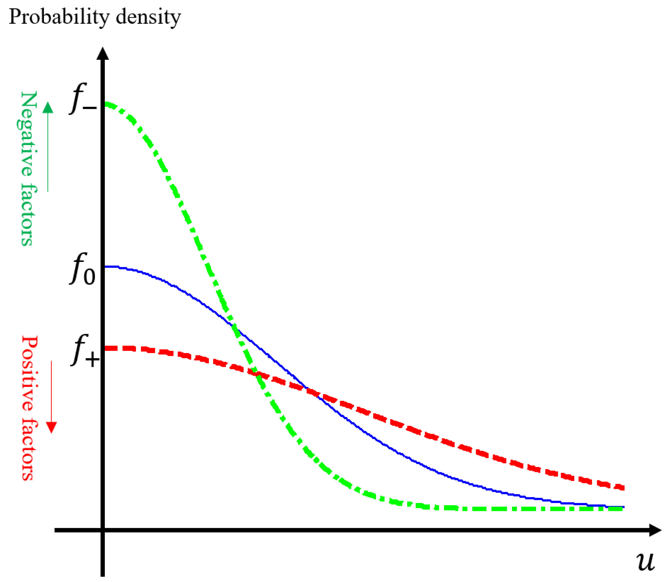
4.1. SFM with Heteroskedasticity

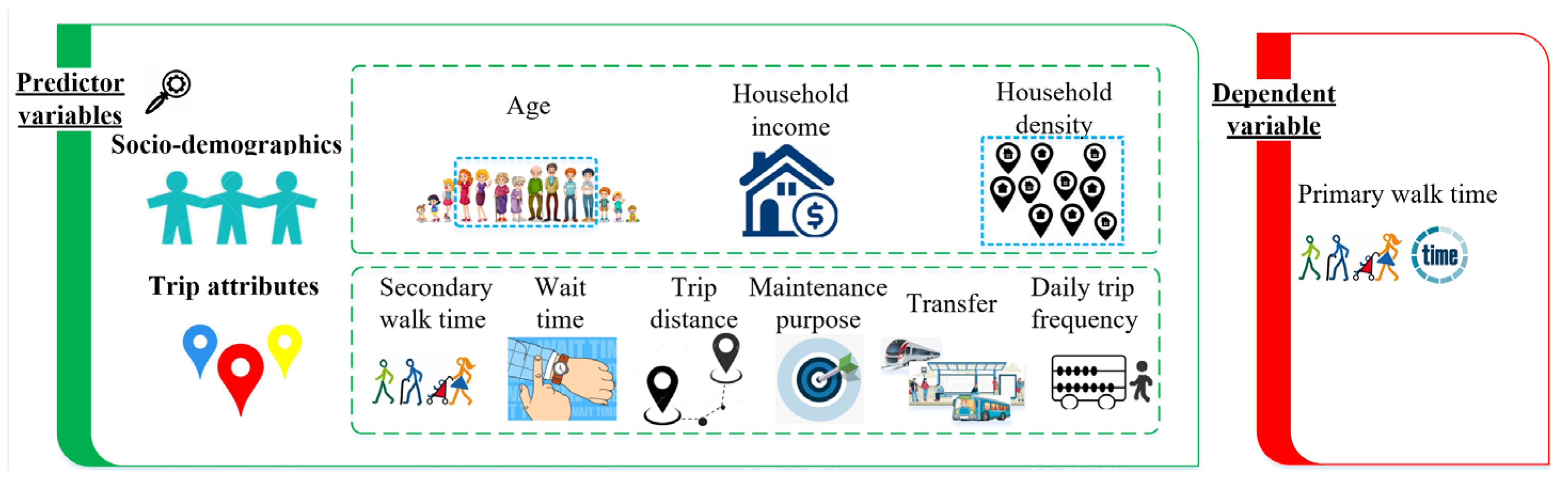
Figure 6 illustrates SFM, where the frontier represents passengers’ unobservable vertex of acceptable stop spacing. The frontier can be estimated with the product of the coefficients and the value of the frontier explanatory variables, which is always no smaller than the primary stop walk time. Thus, the following inequality is established:

$$t\le s_0/v$$

(1)

where $s_0$ is the frontier of acceptable stop spacing, $v$ is the walking speed, and $t$ is the primary walk time, which is given by

$$t=s_0/v-x$$

(2)

where $x$ is a non-negative random variable to represent the gap of the primary walk time from the vertex of walk time.

Such a gap can also be taken as the inefficiency term within the SFM framework, given by

$$Y_i={\beta }^{\prime }{X}_i+v_i-u_i$$

(3)

where $Y_i$ is the primary stop walk time for trip-level observation $i$. ${\beta }^{\prime }{X}_i+v_i$ represents the frontier of acceptable stop walk time: $X_i$ is the vector of frontier explanatory variables, i.e., the factors that decide the maximum acceptable walk time, $\beta$ is the coefficient vector to be estimated, and $v_i$ is random error. $u_i$ is the individual inefficiency that hinders the passenger of trip $i$ from walking the vertex of tolerable walk time. v_i minus $u_i$ is the so-called composite error term.

In the literature on SFM, the random error $v_i$ is typically assumed to be a normal distribution. In contrast, inefficiency term $u_i$ is non-negative, indicating that the observed stop walk time $Y_i$ is always no larger than the vertex of acceptable walk time with a random error, i.e., ${\beta }^{\prime }{X}_i+v_i$. Inefficiency $u_i$ may follow half normal, truncated normal, exponential, or gamma distribution. Taking half normal distribution with heteroskedasticity as an example, the following relationships are developed:

$$u_i~N^{+}\left(0,{\sigma }_{ui}^2\right)$$

(4)

$${\sigma }_{ui}^2=\exp \left(z_i^{\prime }\omega \right)$$

(5)

where ${\sigma }_{ui}^2$ is the variance of the inefficiency term; $z_i$ is a vector of exogenous variables that may include frontier explanatory variables, allowing the hypothesis test whether inefficiency is neutral to frontier predictors; $\omega$ is a vector of coefficients to be estimated.

Variable $z_i$ with a negative coefficient reduces inefficiency variance, vice versa. As demonstrated in Figure 7, the probability of zero inefficiency (i.e., $u=0$) increases with negative factors (i.e., $f_{-}$>$f_{+}$), reducing the gap between the actual and the vertex of stop walk time. The expected value of $u_i$ is given by

$$E\left(u_i\right)={\left(2/\pi \right)}^2\widehat{{\sigma }_u}$$

(6)

where $\widehat{{\sigma }_u}$ is the estimate of ${\sigma }_u$.

4.2. SFM Variables

The SFM dependent variable is the primary stop walk time, as stated at the end of Section 3, to explore passenger tolerance with respect to transit stop spacing. Secondary walk time, i.e., the smaller value between access and egress walk time, is included in the explanatory variables as part of the passenger efforts for transit trips. Other SMF explanatory factors are illustrated below.

Socio-economic attributes include age, household income, and household density. Age is incorporated as young travelers tend to be more active, with generally lower income and better physical strength, contributing to greater tolerance with respect to transit accessibility compared to the busy middle-aged and weak elders [46,47]. Household income has a strong influence on acceptable walk time, as sufficient earnings allow or even demand high-quality trips with moderate stop walk time [48]. Considering that the areas with high residence density are more likely to be served by a fully developed transit service with well-spaced stops [49], transit passengers there are more likely to be accustomed to congenial transit spacing and sensitive to walk time. That is, when walk time is relatively long, habitants there may seek alternative transit routes or alternative trip modes that are more convenient.

Trip characteristics include wait time, trip distance, trip purpose, transfer, and daily trip frequency, in addition to secondary walk time mentioned at the start of Section 4.2. Longer wait time increases transit trip delay to deteriorate service quality, where passengers with longer wait times tend to reduce the acceptable walk distance, so as to avoid excessive delay from transit trips [18,39]. Trip distance also has a significant influence on acceptable stop walk time. Short trips, for example, no longer than 4 km (i.e., 2.5 miles) are open to trip modes other than transit, such as bicycles, taxi, on-line ride-hailing, and private cars [50]. As trip distance increases, the time and cost savings of transit trips increase and make it more attractive, where enlarged stop spacing is easier to be accepted to reduce in-vehicle time [51].

Trip purpose is taken as a predictor variable, which is categorized as maintenance (e.g., shopping, medical, dental, and other family/personal business) or non-maintenance, reflecting the land use type with diverse stop spacing. Thus, trip purpose is binary. Transfer adds to passengers’ physical burden and has been believed to discourage passengers from accepting longer access/egress time [52]. Transfer is also taken as a binary variable, i.e., with or without transfer. Daily trip frequency refers to the total number of trips made by the respondent on the survey day, where frequent trips indicate a more complex activity pattern that is recognized to decrease the usage of unfriendly transit [53], e.g., with excessive walk time. Additionally, as trip frequency increases, the accumulated delay from transit trips also increases, especially when walk time is long, which may trigger a radical change in transit choice [38].

The above non-binary predictors and dependent variables take a natural logarithm, so as to address their heteroskedasticity and non-normal distribution and to quantify the change rate between dependent and independent variables. Taking wait time for example, Figure 8 shows percentile–percentile (P-P) plots to test the normal distribution of the variable and its natural logarithm, where data concentrating along the red line represents a theoretical normal distribution [54]. It is observed that wait time does not obey a normal distribution, but its natural logarithm does, as tested with a skewness and kurtosis of 3.35 and 2.70 vs. −1.75 and 1.34 against a critical value of ±1.96 and ±1.96 [55]. In comparison, binary variables (i.e., trip purpose and transfer) take the form as they are.

Another point worth mentioning is that many other factors have been tested in the study, but only those significant for at least one kind of transit service are presented here and discussed afterward. Other factors that have been tested but are not significant include gender, health level, car ownership, driving license, child presence, education, trip season, life cycle of household, race, being employed or not, and trip day being weekday or weekend. Figure 9 shows the included predictor variables together with a dependent variable, and explanations are given in

Table 3. Variable explanations of the proposed SFM.

Variables	Explanation	Variables	Explanation
Independent
Socio-demographic		Trip attributes
Age	Actual age of the respondent	Secondary walk time	Smaller value between walk access time and walk egress time (min)
Household income	Household income category: 1 = Less than $10,000; 2 = $10,000 to 14,999; 3 = $15,000 to 24,999; 4 = $25,000 to 34,999; 5 = $35,000 to 49,999; 6 = $50,000 to 74,999; 7 = $75,000 to 99,999.	Wait time	Time to wait transit (min)
		Trip distance	Distance between trip origin and destination (mile)
		Maintenance purpose	Binary variable whether the trip is for maintenance purpose or not
Household density	Households per square mile: 50 = 0–99; 300 = 100–499; 750 = 500–999; 1500 = 1000–1999; 3000 = 2000–3999; 7000 = 4000–9999; 17,000 = 10,000–24,999; 30,000 = 25,000–999,999.	Transfer	Binary variable whether there is transfer of the transit trip
		Daily trip frequency	Total trip count on the survey day
Dependent
Primary walk time	Larger value between stop walk access and walk egress time (min)

. Considering that the inferred vertex of transit stop spacing is unobservable, and that the employed 2017 NHTS in the United States is well sampled, there is no need to separate modeling and testing in the following analyses, consistent with the existing literature [43,44].

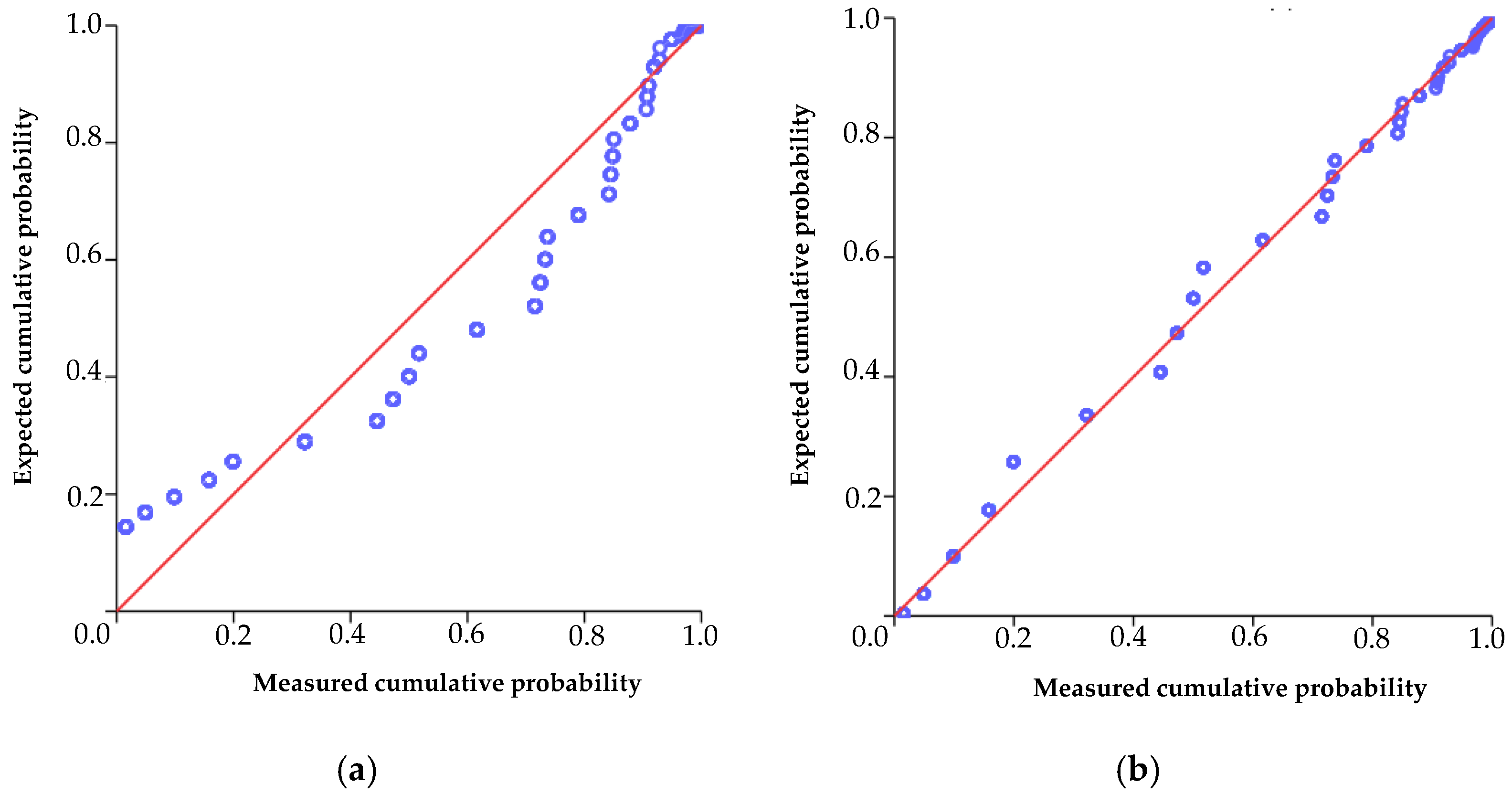
4.3. Solution and Tests

Stata 13.0 was employed to solve the proposed SFM with the command of SFCROSS. Half normal distribution was selected for inefficiency estimation after testing with the PREDICT command. The proposed model was validated with the likelihood ratio, given by

$$LR=-2\times \left[L\left(0\right)-L\left(\beta \right)\right]$$

(7)

as recommended by Kumbhakar et al. [56], where $LR$ means the likelihood ratio, and $L\left(0\right)$ and $L\left(\beta \right)$ represent the log-likelihood values computed from the restricted ordinary least squares (i.e., OLS) and the unrestricted SFM, respectively.

5. Results and Discussions

5.1. Model Results

Table 4. Descriptive statistics of SFM variants.

Variables	R-A Rail Service		Bus Service
			R-A		NR-A
	Mean	Std. Dev	Mean	Std. Dev	Mean	Std. Dev
Independent variable
ln (Age)	3.70	0.36	3.83	0.42	3.75	0.41
ln (Household density)	9.86	0.80	9.61	0.86	8.59	0.95
ln (Household income)	1.87	0.57	1.34	0.78	1.00	0.77
ln (Secondary walk time)	1.44	0.72	1.28	0.80	1.17	0.81
ln (Wait time)	1.78	0.64	2.16	0.74	2.14	0.81
ln (Trip distance)	1.94	0.60	1.57	0.67	1.59	0.66
Maintenance purpose	0.13	0.34	0.25	0.44	0.24	0.43
Transfer	0.36	0.48	0.35	0.48	0.33	0.47
ln (Trip frequency)	0.95	0.40	0.95	0.42	1.01	0.45
Dependent variable
ln (Primary walk time)	2.20	0.71	2.01	0.87	1.98	0.85

shows the descriptive statistics of the predictor and dependent variables. It is observed that the binary variable transfer and the natural logarithms of the household density, household income, and the secondary and primary walk time decrease from R-A rail, to R-A bus, to NR-A bus. Moreover, a larger difference exists between the rail and bus service than between the R-A and NR-A bus service. For example, the natural logarithm of household income is 1.87 for the rail service, while that for the R-A and NR-A bus service is 1.34 and 1.00, respectively. Such a difference indicates the possible gap in SFM factors, as detailed in the following.

Table 5. Estimation of SFM variable coefficients.

Frontier	Rail Service R-A	Bus Service
		R-A	NR-A
ln (Household density)	−0.03 **	−0.04 *	−0.05 ***
ln (Household income)	−0.08 ***	−0.01 *	−0.05 ***
ln (Wait time)	0.12 ***	0.06 *	0.18 ***
ln (Trip distance)	0.25 ***	0.30 ***	0.21 ***
Transfer	0.05	0.11 ***	−0.02
Maintenance purpose	0.08 *	0.09 **	0.10 ***
Constant	2.28 ***	2.17 ***	2.16 ***
Inefficiency variance
ln (Age)	0.45 *	0.21	0.29 *
ln (Wait time)	0.35 **	0.19	0.25 ***
ln (Secondary walk time)	−2.04 ***	−1.85 ***	−2.21 ***
ln (Trip frequency)	0.23	0.17	0.51 ***
Constant	−2.21 **	−1.13	−2.06 ***
Vsigma
Constant	−1.15 ***	−1.13 ***	−1.01 ***
${\sigma }_v$	0.56	0.57	0.60
Statistics
n	2060	1493	2766
${\chi }^2$	177.52 ***	179.96 ***	224.49 ***
$L\left(\beta \right)$	−1950.03	−1669.52	−3031.60
$L(0$)	−2186.43	−1782.98	−3328.76
$LR=-2\left[L\left(0\right)-L\left(\beta \right)\right]$	472.80	226.92	594.32

Note: ***, **, and * means significance at 99%, 95%, and 90% level.

summarizes the SFM results of the R-A rail service and bus service in both R-A and NR-A. It is observed that the value of $LR$ is always much larger than the critical value (i.e., 45) at a 99% significance level [57]. Thus, the proposed SFM is suitable for the estimation of the vertex of transit stop walk time and, as a whole, is highly significant. The estimated frontier stop walk time is averaged to be 13.2, 11.4, and 11.5 min for the rail service, R-A bus service, and NR-A bus service, with the positive difference from the actual primary walk time being 4.2, 3.9, and 4.3 min, respectively. This means that the actual walk distance is smaller than the tolerance vertex by 378, 351, and 387 m (see Figure 10) for the rail service, R-A bus service, and NR-A bus service, respectively, under an average walking speed of 1.5 m/s. Thus, it is indicated that transit agencies in the United States may accordingly enlarge stop spacing as advocated in the existing research [9,16], where acceptable stop spacing for the rail service is largest, while that for the R-A and NR-A bus service is similar.

Thus, this research adds to the literature with an exploration of the vertex of acceptable transit stop spacing based on the inference from the observable transit walk time, instead of empirical statistics [9,10], optimization analysis [20], or a revealed preference survey [27,28,29,30]. Moreover, the result extends previous literature with categorized transit service, finding that the NR-A bus service has the largest gap between the actual stop walk time and its vertex, while the R-A bus service has the smallest. Note that the three gaps are generally close to each other, demonstrating that the transit service there can be enlarged to a similar extent. When transit stop spacing is enlarged accordingly, we may expect to promote a compact, economic, and sustainable transit service without decreasing its accessibility and appeal.

5.2. Frontier Factors

For both the rail and bus service, the coefficients of the natural logarithm of household density and household income are always significantly negative, albeit to a slight extent. For example, when travelers’ household density increases by 1%, stop walk time vertex can be reduced by 0.03%, 0.04%, and 0.05% for the R-A rail, R-A bus, and NR-A bus services, respectively; when household income increases by 1%, walk time vertex can be decreased by 0.08%, 0.01%, and 0.05%. This is because travelers from a household with a satisfying income are capable of choosing comfortable trip modes and only patronizing transit services with a satisfying walk time, and transit services for densely residing areas manage to save travelers from excessive walk time with properly located and spaced transit stops. Thus, passengers in these areas are accustomed to a moderate walk time, instead of tolerating long access/egress time. Thereby, it is recommended to keep congenial transit stop spacing when relocating or removing transit stops in developed areas with higher household income or densely populated areas, consistent with the existing research [48,49].

In contrast, the variables of wait time, trip distance, and maintenance purpose have positive coefficients. That is, travelers who are tolerating long wait times also statistically accept a longer walk time. Specifically, a 1% increase in wait time is related to a 0.12%, 0.06%, and 0.18% increase in the vertex of acceptable walk time for the three transit services. However, excessive spacing can further discourage passengers undergoing long wait times. Therefore, once an alternative trip mode is available, these travelers will no longer use transit. Combined with the finding from existing research that the reduction in bus headway encourages increased walk distance [39], this finding actually reflects the fact that a low-frequency transit service is also featured with sparse stops and requires long walk times, and transit riders thus accept a less attractive service [24,25]. A recommended response measure is to reduce transit wait times with enhanced passenger information system (e.g., published transit schedules and accurate arrival times) and to reduce trip time uncertainty, so as to reduce transit trip delay and maintain service appeal [58]. This is an efficient and economical countermeasure to excessive transit wait times and uncertain transit trip times.

Long-distance travelers also accept longer walk times, with the elasticity coefficient being 0.25, 0.30, and 0.21 for R-A rail, R-A bus, and NR-A bus, respectively, which is consistent with and extends previous research that long-distance travelers prefer larger stop spacing [37]. This can serve long-distance travelers with enlarged stop spacing, where longer access time can be compensated with a reduced in-vehicle time due to less frequent transit pulling in and out [37]. In this case, once passengers are aboard, they may enjoy transit services for a relatively long time and rest, at a friendly transit ticket price.

R-A bus passengers were found with a significantly increased walk time frontier when there is a transfer. That is, the R-A bus transfer can be related to a longer, i.e., 0.11%, walk time frontier. This finding is contradictive to the finding that transfer reduces the acceptable walk time [52,59], which focuses on the transfer impedance but ignores the benefit from transfer such as fare saving and transit coverage extension. Previous research has stated that transit accessibility can be refined with well-designed transfer locations [60]. Therefore, transfer is efficient in enhancing transit mobility and encourages riders to tolerate larger stop spacing. Further, considering that transfer may increase bus wait times and discourage passengers, reducing transfer impedance for the R-A bus service is recommended, e.g., by carefully coordinating the transfer schedule, properly locating transfer stops, and promoting a friendly transfer environment.

In addition, the stop walk time frontier was also statistically increased when serving maintenance trips. Maintenance travelers may be encumbered with elderly or child care or with groceries or luggage. Thus, properly spaced and located transit stops, e.g., close to the entrance and exit of hospitals, banks, and supermarkets, could be a productive avenue of accommodating more maintenance trips. Another interesting finding is that the changes in the walk time frontier from the trip distance are much greater than that from the other factors mentioned above. For example, the elasticity coefficients of trip distance are 0.25, 0.30, and 0.21 vs. 0.08, 0.09, and 0.10 with respect to maintenance purposes for R-A rail, R-A bus, and NR-A bus, respectively. Such a difference assists in the priority decision when stepwisely refining transit stop spacing, where addressing the relationship between trip distance and walk time frontier first is recommended. Figure 11 summarizes the factors of the stop walk time frontier.

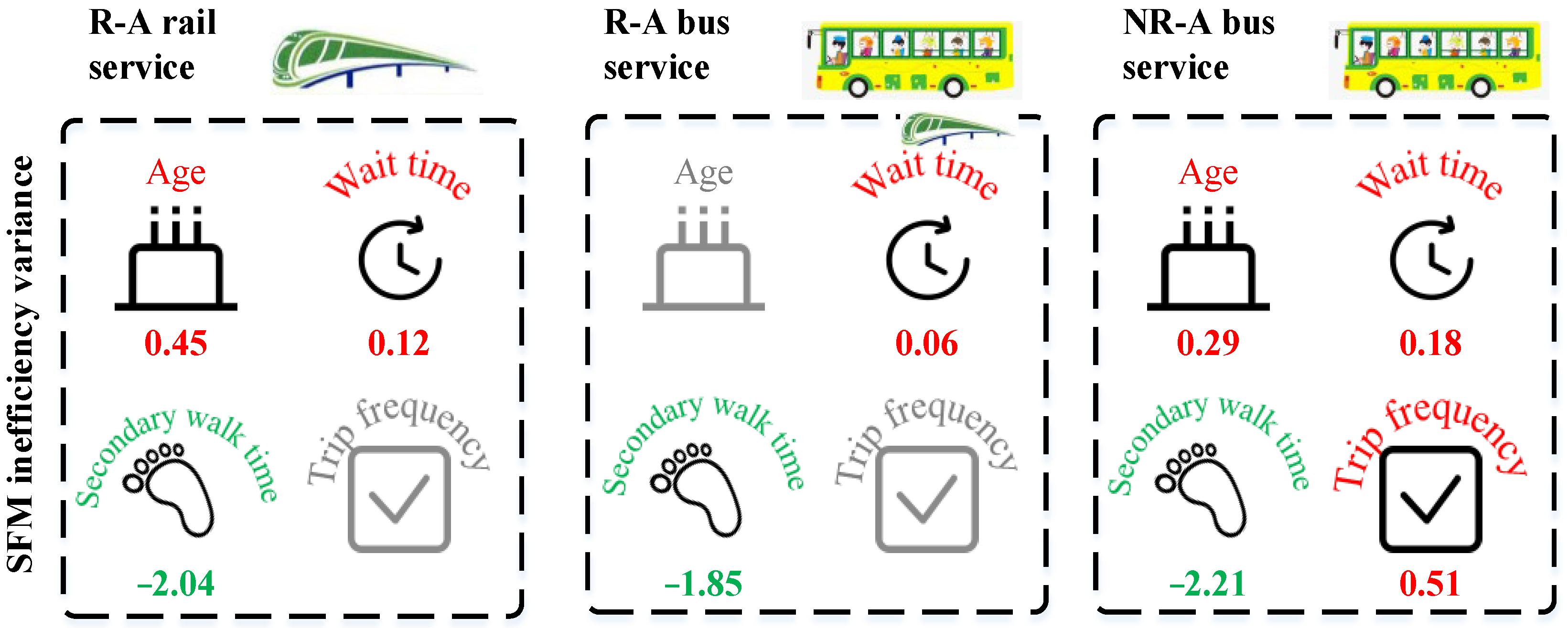
5.3. Inefficiency Variance Factors

Age and wait time have a positive effect on the inefficiency variance for the rail service and the NR-A bus service. That is, when transit passengers are older and wait for longer periods, the natural logarithm of the inefficiency variance is increased by 0.45% and 0.35% for the rail service and by 0.29% and 0.25% for the NR-A bus service. Therefore, the rail service and the NR-A bus service for elderly travelers or those with longer wait times should avoid unnecessarily large stop spacing. Otherwise, the gap between their actual walk time and their vertex of acceptable walk time can increase, and these passengers will be less likely to walk for a longer period towards transit services, as indicated in the existing research [27]. Therefore, when faced with elderly travelers or those with longer wait times, congenial stop spacing is emphasized for transit accessibility, if possible, to avoid unnecessary disappointments in transit usage.

Secondary walk time is negatively related to the inefficiency variance. That is, it helps to maintain passengers’ maximum acceptable walk time. With a 1% increase in secondary walk time, 2.04%, 1.85%, and 2.21% decreases can be observed in the natural logarithm of the efficiency variance to enhance the probability of zero inefficiency. This finding also indicates that the popular practice of large stop spacing in suburban areas and small spacing in urban areas [24,25] fails to exploit passengers’ tolerance with respect to transit accessibility, as it does not well balance the walk time in these areas, which should be better addressed to help retain passengers’ tolerance with respect to stop spacing, instead of focusing only on one specific side. This provides a novel strategy for transit service improvement with respect to balanced walk access and egress time, promoting stable tolerance with respect to the passenger walk vertex.

Moreover, for the NR-A bus service, trip frequency also contributes positively to the walk time inefficiency variance. This is because of the accumulated delay from bus accessibility when faced with frequent trips there. Constrained by the trip schedule to different strict degrees, passenger may be forced to turn to alternative trip modes to reduce access or egress time [38]. In response, when serving travelers frequently using buses or encouraging travelers to ride bus more in NR-A, it is suggested that stop spacing be conservative. Figure 12 summarizes the above findings on the inefficiency variance, where non-significant factors are in gray.

5.4. Discussion

Approximating stop spacing with passenger access or egress time against constant access/egress walking speed, it was found that household density always significantly contributes to a lower stop spacing vertex, where congenial transit accessibility is expected for rail and bus services. A similar finding was observed with respect to household income, which explained travelers’ alternatives for convenient trip modes against well-developed transport system. In contrast, wait time, trip distance, and maintenance purpose are statistically related to a heightened stop spacing vertex for all three kinds of transit service. Wait time is related to both frontier and inefficiency variance for the rail service and the NR-A bus service. As wait time increases, though travelers’ vertex of stop walk time is heightened, the inefficiency variance is also significantly increased. This finding further stresses the previous response strategy that transit wait time should be carefully addressed with enhanced passenger information system (e.g., a published bus schedule and an accurate arrival time), so as to reduce the trip delay and the inefficiency variance and to maintain transit service appeal. Thus, passengers’ tolerance with respect to stop spacing can be better exploited, without forcing them to experience unpleasant trip delays.

Moreover, transit stop spacing can be enlarged for long-distance travelers to reduce their in-vehicle delay from frequent stops and should be carefully addressed for hospitals, banks, supermarkets, etc., so as to facilitate elder and child care as well as luggage carrying. The transfer of R-A bus also significantly extends the stop spacing vertex; transfer impedance should be carefully addressed to reduce transit trip disutility and to maintain service appeal.

Secondary walk time always reduces inefficiency variance for the three kinds of transit, with coefficients as large as −2.04, −1.85, and −2.21, indicating that the access and egress side should be well balanced, instead of focusing only on transit stop spacing. This finding further questions the existing standard of different stop spacing in the dense and sparse areas, and it is advocated to integrate passenger trip behavior into stop spacing design. On the other hand, the passenger age of the rail and NR-A bus service significantly adds to inefficiency variance, and trip frequency is related to increased inefficiency variance only for NR-A bus, promoting the disperse distribution of the inefficiency term. Thus, the actual walk distance by the passengers with such attributes are more likely to be much smaller than the vertex, and it is suggested that stop spacing be adjusted accordingly.

The coefficient of the trip distance for the vertex and the coefficient of secondary walk time for the inefficiency variance are among the largest values compared to other factors, for all three kinds of transit service. Hence, when adjusting transit stop spacing in practice, starting from these two elements is advised. Moreover, considering the hybrid effect of waiting time on both vertex and inefficiency variance, priority to response measures with respect to reducing wait time is also recommended.

Table 6. Significant factors with regard to the frontier and inefficiency terms of acceptable stop spacing.

Frontier	Quantitative	Qualitative
Household density	1% ↑ vs. 0.03%, 0.04%, and 0.05% ↓	Travelers with dense residence expect moderate stop spacing.
Household income	1% ↑ vs. 0.08%, 0.01%, and 0.05% ↓	Travelers with high income patronize transit with moderate stop spacing.
Wait time	1% ↑ vs. 0.12%, 0.06%, and 0.18% ↑	Travelers using low-frequency transit accept larger stop spacing.
Trip distance	1% ↑ vs. 0.25%, 0.30%, and 0.21% ↑	Long-distance travelers accept larger stop spacing.
Transfer	1 vs. 0.05%, 0.11%, and −0.02%↑	Transfer travelers accept larger stop spacing.
Maintenance purpose	1 vs. 0.08%, 0.09%, and 0.10% ↑	Maintenance travelers accept larger stop spacing.
Logarithm of inefficiency variance
Age	1%↑ vs. 0.45%, 0.21%, and 0.29% ↑	As traveler’s age increases, inefficiency variance increases.
Wait time	1%↑ vs. 0.35%, 0.19%, and 0.25% ↑	As traveler’s wait time increases, inefficiency variance increases.
Secondary walk time	1%↑ vs. 2.04%, 1.85%, and 2.21% ↓	As traveler’s secondary walk time increases, inefficiency variance decreases.
Trip frequency	1%↑ vs. 0.23%,0.17%, and 0.51% ↑	As trip frequency increases, inefficiency variance increases.

Note (1) The quantitative explanation is for the rail service and for the R-A and NR-A bus services, respectively. (2) The bold text represents statistical significance.

summarizes the above findings with quantitative and qualitative explanations, where stop walk time is replaced with stop spacing, the gap between which can be bridged with the average walking speed. The findings from this research contribute to quantitatively identifying the key elements in refining transit stop spacing based on passenger travel behavior. Figure 13 further demonstrates the recommended response tool box for determining the acceptable stop spacing of different transit services against various factors, where trip distance and secondary walk time contribute most to the frontier and inefficiency variance, respectively. The findings assist in constructing multi-dimensional implementations for enhanced transit stop spacing, for service accessibility, which can help to retain and even increase ridership, and for operation efficiency, which can help to reduce service costs and deficits.

6. Conclusions

Stop spacing is critical to transit service quality and coverage as well as operation cost, the determinants of transit sustainability. Though tremendous efforts have been devoted to this issue, there is still great inconsistency in stop spacing standards. Moreover, the widely adopted categorization of stop spacing by land use is deficient, as frequent stops in downtown dramatically increase in-vehicle passenger delay, while inaccessible service in the underserved areas may deteriorate captive riders’ situation. This research adds to the literature by developing SFM to infer passengers’ unobservable tolerance with respect to stop spacing based on trip-level passenger behaviors, which integrates passenger socio-demographics and trip characteristics into a unified framework, referring to the 2017 NHTS in the United States.

Given the significant difference between rail and bus service, and the difference in the areas with and without heavy rail, transit service is categorized as an R-A rail service, an R-A bus service, or an NR-A bus service, supported by sufficient data. With primary stop walk time, the vertex of transit stop spacing is represented at the trip level against the predictors of rider age, household income, household density, secondary walk time, wait time, trip distance, maintenance purpose, transfer, and daily trip frequency. The significant explanatory variables on the vertex of acceptable transit stop spacing are identified with their quantified impacts, including household income, household density, wait time, trip distance, transfer, and maintenance purpose. Inefficiency variance is validated to be significantly related to traveler age, wait time, secondary walk time, and trip frequency. Response strategies are proposed to provide insights, guidelines, and implementation plans for different transit agencies when considering stop spacing redesign, to strengthen transit service appeal, and to promote a cooperative and sustainable multi-modal urban transport system.

The applicability to other countries and areas of the findings based on the 2017 NHTS in the United States needs further exploration, especially against different economic and cultural conditions. Furthermore, further efforts are necessary, as the factors that influence transit usage are multi-dimensional and could be more complex than we have presented. Specifically, the data from the NHTS does not include concrete trip information such as transit route and boarding or alighting stops, nor the information of origin and destination. Thus, the model based on the simplified data may leave out important factors and bias the results, into which deep digging is encouraged for a comprehensive understanding of acceptable stop walk time. Additionally, the empirical performance of the recommendations from this research, i.e., to enlarge stop spacing for the specified passenger groups, needs further validation, which is necessary before the findings are incorporated into guides on transit development. Given the rapid development of shared mobility, a fruitful avenue for further research is to investigate ways to combine these modes with transit into a unified urban transport system and to explore the resultant changes in acceptable service spacing, so as to promote a seamless and well-organized transportation system for a sustainable city life.

References

1. Dano, U.L.; Balogun, A.L.; Abubakar, I.R.; Aina, Y.A. Transformative urban governance: Confronting urbanization challenges with geospatial technologies in Lagos, Nigeria. GeoJournal 2020, 85, 1039–1056. [Google Scholar] [CrossRef]
2. Boisjoly, G.; Grisé, E.; Maguire, M.; Veillette, M.P.; Deboosere, R.; Berrebi, E.; El-Geneidy, A. Invest in the ride: A 14 year longitudinal analysis of the determinants of public transport ridership in 25 North American cities. Transp. Res. Part A Policy Pract. 2018, 116, 434–445. [Google Scholar] [CrossRef]
3. Clewlow, R.R.; Mishra, G.S. Disruptive Transportation: The Adoption, Utilization, and Impacts of Ride-Hailing in the United States; Institute of Transportation Studies, University of California: Davis, CA, USA, 2017. [Google Scholar]
4. Yang, H.; Qin, X.; Ke, J.; Ye, J. Optimizing matching time interval and matching radius in on-demand ride-sourcing markets. Transp. Res. Part B Methodol. 2020, 131, 84–105. [Google Scholar] [CrossRef]
5. Zhao, J.; Sun, S.; Cats, O. Joint optimisation of regular and demand responsive transit services. Transp. A Transp. Sci. 2021, 1–24. [Google Scholar] [CrossRef]
6. Rayle, L.; Dai, D.; Chan, N.; Cerveroa, R.; Shaheen, S. Just a better taxi? A survey-based comparison of taxis, transit, and ridesourcing services in San Francisco. Transp. Policy 2016, 45, 168–178. [Google Scholar] [CrossRef] [Green Version]
7. Tirachini, A. The economics and engineering of bus stops: Spacing, design and congestion. Transp. Res. Part A Policy Pract. 2014, 59, 37–57. [Google Scholar] [CrossRef]
8. Li, J. Residential and transit decisions: Insights from focus groups of neighborhoods around transit stations. Transp. Policy 2018, 63, 1–9. [Google Scholar] [CrossRef]
9. Maryland Transit Administration. Bus Stop Optimization Policy (Pilot); Maryland Department of Transportation: Hanover, MA, USA, 2014.
10. Transport for London. Travel in London Report 9; Mayor of London: London, UK, 2016.
11. Zhao, J.; Zhou, X. Improving the operational efficiency of buses with dynamic use of exclusive bus lane at isolated intersections. IEEE Trans. Intell. Transp. Syst. 2018, 20, 642–653. [Google Scholar] [CrossRef]
12. TCRP Report. Transit Capacity and Quality of Service Manual, 3rd ed.; Transportation Research Board: Washington, DC, USA, 2013; Chapter 3. [Google Scholar]
13. Kittelson, A. Federal Transit Administration; Transit Cooperative Research Program; Transit Development Corporation. In Transit Capacity and Quality of Service Manual; Transportation Research Board: Washington, DC, USA, 2013. [Google Scholar]
14. Ammons, D.N. Municipal Benchmarks: Assessing Local Performance and Establishing Community Standards, 2nd ed.; Sage: Thousand Oaks, CA, USA, 2001. [Google Scholar]
15. Walker, J. Human Transit: How Clearer Thinking about Public Transit Can Enrich Our Communities and Our Lives; Island Press: Washington, DC, USA, 2012. [Google Scholar]
16. Reilly, J.M. Transit Service Design and Operation Practices in Western European Countries. Transp. Res. Rec. J. Transp. Res. Board. 1997, 1604, 3–8. [Google Scholar] [CrossRef]
17. Vuchic, V.R.; Newell, G.F. Rapid transit interstation spacings for minimum travel time. Transp. Sci. 1968, 2, 303–339. [Google Scholar] [CrossRef]
18. O’Sullivan, S.; Morrall, J. Walking distances to and from light-rail transit stations. Transp. Res. Rec. 1996, 1538, 19–26. [Google Scholar] [CrossRef]
19. Baum-Snow, N.; Kahn, M.E. The effects of new public projects to expand urban rail transit. J. Public Econ. 2000, 77, 241–263. [Google Scholar] [CrossRef]
20. Nes, R.V.; Bovy, P. Importance of objectives in urban transit-network design. Transp. Res. Rec. 2000, 1735, 25–34. [Google Scholar]
21. Greenville Transit Authority. Bus Stops Procedure Manual; Government of Greenville: Greenville, CA, USA, 2017.
22. Public Transportation Boosts Property Values. Available online: https://www.nar.realtor/articles/public-transportation-boosts-property-values (accessed on 20 April 2022).
23. Flyvbjerg, B.; Bruzelius, N.; van Wee, B. Comparison of capital costs per route-kilometre in urban rail. arXiv 2013, arXiv:1303.6569. [Google Scholar]
24. Johnson, D.; Ercolani, M.; Mackie, P. Econometric analysis of the link between public transport accessibility and employment. Transport. Policy 2017, 60, 1–9. [Google Scholar] [CrossRef]
25. Kramer, A. The unaffordable city: Housing and transit in North American cities. Cities 2018, 83, 1–10. [Google Scholar] [CrossRef]
26. Hossain, M.S.; Hunt, J.D.; Wirasinghe, S.C. Nature of influence of out-of-vehicle time-related attributes on transit attractiveness: A random parameters logit model analysis. J. Adv. Transp. 2015, 49, 648–662. [Google Scholar] [CrossRef]
27. Kim, J.; Kim, J.; Jun, M.; Kho, S. Determination of a bus service coverage area reflecting passenger attributes. J. East. Asia Soc. Transp. Studies 2005, 6, 529–543. [Google Scholar]
28. Kim, K.W.; Lee, D.W. A model to estimate the marginal walking time of bus users by using adaptive neuro-fuzzy inference system. KSCE J. Civ. Eng. 2008, 12, 197–204. [Google Scholar] [CrossRef]
29. Kim, K.W.; Lee, D.W.; Chun, Y.H. A comparative study on the service coverages of subways and buses. KSCE J. Civ. Eng. 2010, 14, 915–922. [Google Scholar] [CrossRef]
30. Samimi, A.; Ermagun, A. Students’ tendency to walk to school: Case study of Tehran. J. Urban. Plan. Dev. 2012, 139, 144–152. [Google Scholar] [CrossRef] [Green Version]
31. O’Connor, D.; Caulfield, B. Level of service and the transit neighbourhood-Observations from Dublin city and suburbs. Res. Transp. Econ. 2018, 69, 59–67. [Google Scholar] [CrossRef] [Green Version]
32. McIntosh, J.; Trubka, R.; Newman, P. Can value capture work in a car dependent city? Willingness to pay for transit access in Perth, Western Australia. Transp. Res. Part A Policy Pract. 2014, 67, 320–339. [Google Scholar] [CrossRef]
33. Jiang, Y.; Zegras, P.C.; Mehndiratta, S. Walk the line: Station context, corridor type and bus rapid transit walk access in Jinan, China. J. Transp. Geogr. 2012, 20, 1–14. [Google Scholar] [CrossRef]
34. Pueboobpaphan, R.; Pueboobpaphan, S.; Sukhotra, S. Acceptable walking distance to transit stations in Bangkok, Thailand: Application of a stated preference technique. J. Transport. Geogr. 2022, 99, 103296. [Google Scholar] [CrossRef]
35. Bowman, J.L.; Ben-Akiva, M.E. Activity-based disaggregate travel demand model system with activity schedules. Transp. Res. Part A Policy Pract. 2001, 35, 1–28. [Google Scholar] [CrossRef]
36. Pinjari, A.R.; Pendyala, R.M.; Bhat, C.R.; Waddell, P.A. Modeling the choice continuum: An integrated model of residential location, auto ownership, bicycle ownership, and commute tour mode choice decisions. Transportation 2011, 38, 933. [Google Scholar] [CrossRef] [Green Version]
37. Office of Transit System Planning. MARTA Service Standards; Metropolitan Atlanta Rapid Transit Authority: Atlanta, GA, USA, 2018. [Google Scholar]
38. Cohen, S.; Yannis, G. Traffic Management; ISTE Ltd: London, UK, 2016. [Google Scholar]
39. Mulley, C.; Ho, C.; Ho, L.; Hensher, D.; Rose, J. Will bus travelers walk further for a more frequent service? An international study using a stated preference approach. Transport. Policy 2018, 69, 88–97. [Google Scholar] [CrossRef] [Green Version]
40. Kitamura, R.; Yamamoto, T.; Kishizawa, K.; Pendyala, R.M. Stochastic frontier models of prism vertices. Transp. Res. Rec. 2000, 1718, 18–26. [Google Scholar] [CrossRef]
41. Hamjah, M.A. Climatic Effects on Cotton and Tea Productions in Bangladesh and Measuring Efficiency using Multiple Regression and Stochastic Frontier Model Respectively. Math. Theory Modeling 2014, 4, 86–98. [Google Scholar]
42. Federal Highway Administration. National Household Travel Survey; United States Department of Transportation: Washington, DC, USA, 2017.
43. Wiegmans, B.; Witte, P. Efficiency of inland waterway container terminals: Stochastic frontier and data envelopment analysis to analyze the capacity design—And throughput efficiency. Transp. Res. Part A Policy Pract. 2017, 106, 12–21. [Google Scholar] [CrossRef] [Green Version]
44. Susilo, Y.O.; Avineri, E. The impacts of household structure on the individual stochastic travel and out-of-home activity time budgets. J. Adv. Transp. 2014, 48, 454–470. [Google Scholar] [CrossRef] [Green Version]
45. Owen, A.; Levinson, D.M. Modeling the commute mode share of transit using continuous accessibility to jobs. Transp. Res. Part A Policy Pract. 2015, 74, 110–122. [Google Scholar] [CrossRef] [Green Version]
46. Alsnih, R.; Hensher, D.A. The mobility and accessibility expectations of seniors in an aging population. Transp. Res. Part A Policy Pract. 2003, 37, 903–916. [Google Scholar] [CrossRef]
47. Jin, H.; Yu, J. Gender Responsiveness in Public Transit: Evidence from the 2017 US National Household Travel Survey. J. Urban. Plan. Dev. 2021, 147, 04021021. [Google Scholar] [CrossRef]
48. Tian, G.; Ewing, R. A walk trip generation model for Portland, OR. Transp. Res. Part D Transp. Environ. 2017, 52, 340–353. [Google Scholar] [CrossRef]
49. Lewis, S. Neighborhood density and travel mode: New survey findings for high densities. Int. J. Sustain. Dev. World Ecology 2018, 25, 152–165. [Google Scholar] [CrossRef]
50. Feigon, S.; Murphy, C. Broadening Understanding of the Interplay between Public Transit, Shared Mobility, and Personal Automobiles; Transportion Research Board: Washington, DC, USA, 2018. [Google Scholar]
51. Daganzo, C.F. Structure of competitive transit networks. Transp. Res. Part. B Methodol. 2010, 44, 434–446. [Google Scholar] [CrossRef] [Green Version]
52. Iseki, H.; Taylor, B.D. Not all transfers are created equal: Towards a framework relating transfer connectivity to travel behaviour. Transp. Rev. 2009, 29, 777–800. [Google Scholar] [CrossRef]
53. Hensher, D.A.; Reyes, A.J. Trip chaining as a barrier to the propensity to use public transport. Transportation 2000, 27, 341–361. [Google Scholar] [CrossRef]
54. Boylan, G.L.; Cho, B.R. The normal probability plot as a tool for understanding data: A shape analysis from the perspective of skewness, kurtosis, and variability. Qual. Reliab. Eng. Int. 2012, 28, 249–264. [Google Scholar] [CrossRef]
55. Bai, J.; Ng, S. Tests for skewness, kurtosis, and normality for time series data. J. Bus. Econ. Stat. 2005, 23, 49–60. [Google Scholar] [CrossRef] [Green Version]
56. Kumbhakar, S.C.; Wang, H.; Horncastle, A.P. A Practitioner’s Guide to Stochastic Frontier Analysis Using Stata; Cambridge University Press: Cambridge, UK, 2015. [Google Scholar]
57. Kodde, D.A.; Ritzen, J.M. Direct and indirect effects of parental education level on the demand for higher education. J. Hum. Resour. 1988, 356–371. [Google Scholar] [CrossRef]
58. Wong, J. Leveraging the general transit feed specification for efficient transit analysis. Transp. Res. Record 2013, 2338, 11–19. [Google Scholar] [CrossRef]
59. Ibrahim, M.F. Car ownership and attitudes towards transport modes for shopping purposes in Singapore. Transportation 2003, 30, 435–457. [Google Scholar] [CrossRef]
60. Chia, J.; Lee, J.B. Extending public transit accessibility models to recognize transfer location. J. Transport. Geogr. 2020, 82, 102618. [Google Scholar] [CrossRef]
Figure 1. Illustration of transit trips.
Sustainability 14 06148 g001
Figure 2. Illustration of three kinds of transit trips. (a) Rail service of R-A; (b) Bus service of R-A; (c) Bus service of NR-A.
Sustainability 14 06148 g002
Figure 3. Illustration of transit stop spacing and access/egress time.
Sustainability 14 06148 g003
Figure 4. Share of feeder modes for transit service. (a) Access mode share; (b) egress mode share.
Sustainability 14 06148 g004
Figure 5. Illustration of secondary, primary, and vertex of acceptable stop walk time.
Sustainability 14 06148 g005
Figure 6. Illustration of SFM results.
Sustainability 14 06148 g006
Figure 7. Distribution of inefficiency term.
Sustainability 14 06148 g007
Figure 8. P-P plots of wait time and its natural logarithm. (a) Wait time; (b) In (Wait time).
Sustainability 14 06148 g008
Figure 9. Illustration of predictor and dependent variables.
Sustainability 14 06148 g009
Figure 10. Gap between primary walk time and the vertex of walk time.
Sustainability 14 06148 g010
Figure 11. Frontier factors of the stop walk time.
Sustainability 14 06148 g011
Figure 12. Factors of inefficiency variance for stop walk time.
Sustainability 14 06148 g012
Figure 13. Recommended response tool box for the acceptable stop spacing of different transit service.
Sustainability 14 06148 g013