Sustainable Development–Fiscal Federalism Nexus: A “Beyond GDP” Approach

Abstract

The hypothetical allocative efficiency of fiscal federalism and its potential welfare impact have fueled the increased fiscal authority of subnational governments experienced in most countries around the world. This research sheds light on important aspects of developmental outcome of fiscal federalism which hitherto either have not been explored or have been obscured by the exclusive use of GDP or GDP growth as the empirical measure of welfare and development in previous studies. The National Sustainable Development Index (NSDI) and its subcomponent indices were computed for 40 selected countries from 2006 to 2018. Using the NSDI as welfare proxy and employing the difference and system generalized method of moments techniques, this study revealed that fiscal federalism has no significant impact on aggregate sustainable development, environmental and natural resource development index, and social development index, but has a positive impact on economic development index. Hence, fiscal federalism discourse among policy decision-makers in most countries seems to have been based on economic development considerations, leaving out other important dimensions of sustainable development. Therefore, in designing a fiscal federalism apparatus, policy decision-makers should consider proper coordination of the three dimensions of sustainable development if the development-enhancing role of fiscal federalism is to be sustainably achieved.

1. Introduction

“In order for development to be sustainable, it has to be comprehensive–it has to successfully balance economic growth with social and environmental.” (Extract from “Beyond Economic Growth”, student book by World Bank, 2004).

The environmental and social problems which accompany rapid global development of economy and society have become increasingly serious and of much concern. The only solution to solve the environmental, social, and economic growth dilemma is sustainable development. This has led many countries and international organizations to put forward plans or goals for sustainable development [1] A notable and most recent international plan in this direction is the United Nation 2030 Agenda for Sustainable Development (UN Agenda 2030), which was unanimously adopted by all 193 member states in September 2015. The agenda is comprised of 17 Sustainable Development Goals (SDGs) and 169 targets, which came into effect on 1 January 2016. It is an ambitious international move towards sustainable development and beyond the GDP or mere economic growth as a measure of welfare. The UN described the agenda as unprecedented in scope and significance, and stated that “it is accepted by all countries and is applicable to all, taking into account different national realities, capacities and levels of development and respecting national policies and priorities.”

Sustainable development is a multidiscipline and multidimensional concept. It originated from ecology but has also become a main subject matter in economics, environmental science, and sociology [2,3]. Although these various disciplines study the concept from different perspectives, the essence and goals are the same for them [4]. The main goal of sustainable development is the maximization of intergenerational utility. In other words, the concept of sustainable development requires that economic, social, and environmental development should be coordinated with the objective of balancing intragenerational welfare and maximizing the total welfare of all generations [4]. In fact, the Brundtland report, Our Common Future (Brundtland report published in 1987 and named after the former prime minister of Norway, Gro Harlem Brundtland who chaired the World Commission of Environment and Development (set up in 1983)) defines sustainable development as “Development that meets the needs of the present without compromising the ability of the future generations to meet their own needs.” Hence, according to the sustainable development concept, economic growth and social progress should be pursued to ensure the welfare of present generations, while protecting the ecological environment and rationally utilizing natural resources to ensure the welfare of future generations. Pursuing economic growth at the detriment of the environment and natural resource utilization is not sustainable development. Protecting the environment while making the economy stagnate would also not be a sustainable development mode [1].

In line with the above-mentioned goal of sustainable development, the UN explained that the Sustainable Development Goals and the associated targets are integrated and indivisible, and the goals and targets balance the three dimensions of sustainable development: economic, social, and environmental. It stated further that the governments and representatives who put forward the UN Agenda 2030 are committed to achieving sustainable development in its three dimensions in a balanced and integrated manner, and that the agenda will be implemented for the full benefit of all, for present generation and for future generations. The Sustainable Development Goals are to be attained through governments’ decision-making processes, including policies, plans, programs, and projects. Moreover, for the actualization of the UN Agenda 2030, the UN calls for the development of broader measures of welfare and progress to complement Gross Domestic Product (GDP), the consultation and inclusion of all relevant stakeholders, and the recognition and exploration of link between sustainable development and other relevant ongoing processes in the economic, social, and environmental fields. To this end, the study aims to compute the National Sustainable Development Index (NSDI) and its subcomponent indices for the selected sample countries. In addition, the last three decades have witnessed an increase in the fiscal authority of the subnational governments in most countries [5]. However, not only is it that there is lack of empirical consensus on the welfare effects of fiscal decentralization, but also, little attention has been given to the impact of fiscal federalism on development beyond GDP.

Consequently, this paper wishes to shed further light on important aspects of the relationship between development and fiscal federalism which hitherto either have not been explored or have been obscured by the exclusive use of GDP or GDP growth as the empirical measure of welfare and development in previous studies. To achieve this, the study uses a panel data set of 40 countries, including 11 federations and 29 non-federations over the period 2006 to 2018. Moreover, 17 of the countries are developed and 23 are developing countries, the choice of countries being determined by the constraint of data availability, especially the data on the fiscal federalism measures. Particularly, the study hypothesizes and tests the impact of fiscal federalism on sustainable development at the aggregate level, and its impact on the various dimensions of sustainable development at a disaggregated level. The rest of the paper is structured as follows. Section 2 reviews the theoretical and empirical literatures on the relationship between fiscal federalism and sustainable development. Section 3 describes the data and variables used in the empirical analysis. The empirical framework and methodology are presented in Section 4. Section 5 discusses the empirical results, followed by a conclusion and policy implications in Section 6.

2. Literature Review

Based on existing theory, fiscal federalism may be a factor influencing sustainable development. Fiscal federalism aims at deriving principles that can be used to determine the optimal allocation of fiscal functions among the different tiers of government in a federation. However, in recent times, the application and practice of fiscal federalism is not limited to federation, as both federal and unitary countries are now embracing the design of some form of fiscal decentralization between the central and subcentral governments. The framework for what became accepted as the proper role of the state in the economy was provided by Samuelson’s two important papers [6,7] on the theory of public goods, Musgrave’s book [8] on public finance, and Arrows discourse [9] on the roles of the public and private sectors. Their arguments are based on the public finance trio of allocative efficiency, distributive equity, and stabilization. It was opined that the allocative role is best performed by the subnational governments while the distributive equity and stabilization roles are best performed by the central government. Furthermore, Tiebout [10] hypothesizes that in a situation where it is efficient to have multiple jurisdictions providing local public goods, then inter-jurisdictional competition for residents will lead to a near-optimal outcome. Tiebout [10] argues that jurisdictions can acquire more residents either by acting as a cartel, imposing singular tax rate on the residents, or by engaging in tax competition. Tiebout [10] claims that the end result of both approaches will be the same because the tax rates of the various jurisdictions will converge around an average tax rate, even in the case of inter-jurisdictional tax competition. The implication of Tiebout’s hypothesis is that as a result of competition for residents by subnational governments, fiscal federalism will lead to allocative efficiency, which will in turn lead to sustainable development. Moreover, Kalirajan and Otsuka [11] drawing from Oates [12] argues that “in an ideal decentralized system, existing resources will be allocated to yield the maximum possible output (locating on the production possibility frontiers) and the competitive environment including inter-governmental competition will be conducive for technological progress (shift in the frontier).” This also implies that fiscal federalism has a positive developmental outcome. This is the view of the so-called “traditional” or “first-generation theory of fiscal federalism.” This approach assumes that the public decision-makers are benevolent agents who choose to maximize the social welfare of the citizens [13]. On the other hand, the so-called “second-generation theory of fiscal federalism” assumes that public decision-makers usually have goals which are induced by political institutions that often diverge from maximizing the welfare of the citizens. They therefore argue that fiscal federalism could have varied, and not necessarily a positive developmental outcome [13,14,15,16].

In relation to the empirical literature on sustainable development impact of fiscal federalism, there are two limitations. One is that most of the research on the developmental output of fiscal federalism is based on the impact of fiscal federalism on economic growth, using GDP or GDP growth rate as a measure of welfare, and fiscal federalism has been given little or no consideration in most of the studies on the determinants of sustainable development. The other is that most hitherto used proxies for sustainable development are not as comprehensive as the NSDI employed in this study. The argument that fiscal federalism foster economic growth and development through allocative efficiency has been the main reason most countries tend towards more fiscally decentralized economy in recent times. This has also been the reason for much empirical research on the fiscal federalism–developmental outcome nexus. Moreover, the measure of developmental outcome has been restricted to economic growth or development measured by GDP per capita or GDP per capita growth rate. However, the serious social and environmental challenges which accompany economic growth give rise to a dilemma in sustainable development, which in its holistic view comprises of the economic development, social development, and environmental development. This is the reason many countries, organizations, and interested parties are clamoring for the need to see development beyond just economic development, but as one that is comprehensive, balanced, and well-coordinated in the three dimensions of sustainable development [17,18]. Furthermore, in its 2020 report, the UN-Habitat estimates that 23 percent of the Sustainable Development Goal indicators have a component which is local or urban, and the OECD economic outlook states that 105 of the 169 sustainable development targets, which underline the 17 Sustainable Development Goals would not be reached without the proper coordination and engagement of the subnational governments [19]. Thus, it is imperative to investigate the impact that the recent resurgence of interest in fiscal federalism will have on sustainable development. This argument is not based on political decentralization or political decisions, but on fiscal decentralization, which the Tiebout-sorting hypothesis and other theoretical literature on the link between fiscal federalism and developmental outcome through allocative efficiency deal with.

The literature on the relationship between fiscal federalism and economic activities is vast and mixed: some studies found a clear positive relationship, e.g., [20,21,22,23,24,25,26]; some found negative relationships, e.g., [27,28,29,30,31]; while several others found no relationship at all, e.g., [32]. Traditional literature on fiscal federalism [6,7,8,9,12,33] posit that fiscal decentralization has a positive effect on economic activities. However, some more recent literature argues that fiscal decentralization can pose a significant risk and worsen macroeconomic problems [34,35,36,37,38,39]. Blöchliger et al. [40] opine that the relationship between fiscal federalism and economic activities could indeed be non-linear, with the positive effects fading out as the level of fiscal decentralization increases. They found evidence of a hump-shaped relationship, which portrays a level of “optimal decentralization” beyond which additional decentralization will inhibit rather than foster economic activities. Their argument on the idea of “optimal decentralization” is based on the fact that negative factors such as diseconomies of scale and scope, internal trade barriers, distorting local tax systems, rent seeking of local vested interests, and other negative implications of decentralized policymaking might overwhelm the positive aspects once decentralization extends beyond a critical level. However, in all of the aforementioned studies, the social and the environmental and resource dimensions of sustainable development were not considered. In addition, the economic dimension was restricted to economic growth only.

On the determinants of sustainable development, the potential roles of a number of factors have been considered by a growing body of literature. Non-renewable energy consumption and excessive dependence on natural resources have been found to be inconducive to sustainable development [41,42]. Human capital, higher education, democracy, social fairness, and positive institutional environment have been established to have positive impacts on sustainable development [43,44]. Additionally, Reiter and Steensma [45] established the impact on sustainable development of corruption, quality of governance, legal system, violent conflict, and foreign direct investment. Moreover, a number of studies have established the influence of several aspects of fiscal policy on sustainable development [46,47,48]. The only notable study that has considered the impact of fiscal federalism on sustainable development is Jin and Martinez-Vasquez [1]. Using the National Sustainable Development Index as the measure of sustainable development, and panel data of 52 countries, the study argued that there is a hump-shaped relationship between expenditure decentralization and sustainable development.

This study is motivated and warranted by two main reasons: (i) the call by the UN for the consultation and inclusion of all relevant stakeholders, and the recognition and exploration of link between sustainable development and other relevant ongoing processes in the economic, social, and environmental fields towards the achievement of the UN Agenda 2030, and (ii) the very limited attention that has been given in the literature to the study of the relationship between fiscal federalism and sustainable development, despite the fact that in recent times, there has been an increase in the role of subnational government in most countries. Hence, in line with Jin and Martinez-Vasquez [1], this study examines the impact of fiscal federalism on sustainable development using the National Sustainable Development Index (NSDI) as the proxy for sustainable development.

However, unlike Jin and Martinez-Vasquez [1] which set out with the sole aim of verifying an assumed hump-shaped relationship between expenditure decentralization and sustainable development, this study does not assume an already established relationship between fiscal federalism and sustainable development but seeks to determine if a relationship exists or not and take into consideration both revenue decentralization and expenditure decentralization. Moreover, Jin and Martinez-Vasquez [1] uses the two-stage least square estimation technique with the Geographic Fragmentation Index as instrumental variable in their analysis and make use of a five-year average panel data. The Geographic Fragmentation Index is only available for years 1990, 1995, 2000, and 2010, and it is argued that in dealing with endogeneity in a dynamic panel data, the IV approach does not exploit all of the information available in the sample [49]. The five- year average is also argued to lead to a loss of degree of freedom, and consequently reduced efficiency of the regression estimates. This study makes use of the difference and system generalized method of moment estimators which is a more robust technique that produces a more efficient estimates of the dynamic panel data model [49]. This could be the reason for the difference between the findings of the Jin and Martinez-Vasquez [1] and the findings in this study concerning the sustainable development impact of fiscal federalism on the aggregate. The study also investigates the impact of fiscal federalism on each of the three dimensions of sustainable development separately. Furthermore, the study examines if the Kuznets’s hypothesis exists for the relationship between fiscal federalism and sustainable development, and investigates if the sustainable development impact of fiscal federalism varies between federal and non-federal countries. Moreover, as a check of robustness and for comparative purposes, the study explores the impact of fiscal federalism on Human Development Index (HDI) and GDP growth rate. HDI being the most popular measure of sustainable development and GDP growth rate being the most used measure of welfare in most studies on developmental outcome of fiscal federalism.

Therefore, the aim of this paper is to shed some light on the relationship between fiscal federalism and sustainable development. In this regard, this study chooses to provide answers to the following research questions: what is the impact of fiscal federalism on sustainable development? What is the impact of fiscal federalism on the various dimensions of sustainable development? What is the influence of a nation being a federation on sustainable development impact of fiscal federalism? These research questions were explored using the difference and system generalized method-of-moments (GMM) estimators.

3. Data and Variable Definition

This section describes the data and variables used in the empirical analysis. The study uses a panel data set of 40 countries, which includes 11 federations and 29 non-federations over the period 2006 to 2018. The selection of countries and the choice of sample under investigation were dictated by two main factors: (i) availability of adequate and accurate data on the indicators required to compute the National Sustainable Development Index, (ii) sufficient data availability for the fiscal federalism indicators and the control variables for the countries. All the data used for the empirical analysis were sourced from the World Bank online database. The main intent of the study is to investigate the impact of fiscal federalism on sustainable development while controlling for other determinants of sustainable development. The variables used in the analysis are described below.

3.1. Dependent Variable

The main dependent variable used in the analysis as a proxy for sustainable development is the National Sustainable Development Index (NSDI). The NSDI is a composite index initially proposed by Jin et al. [4] and upgraded by Jin and Martinez-Vazquez [1]. The index was proposed in response to the UN 2030 Agenda for Sustainable Development (UN Agenda 2030) call for the development of broader measures of welfare and progress to complement Gross Domestic Product (GDP). This index, which is built on the economic, social, and environmental and resource dimensions of sustainable development using 12 indicators, is also an improvement over previously constructed alternatives to GDP such as the Human Development Index (HDI). The indicators used are based on the Sustainable Development Goals (SDGs) (See

Table A1. The United Nation’s Sustainable Development Goals—UN 2030 Agenda.

Sustainable Development Goals
Goal 1. End poverty in all its forms everywhere
Goal 2. End hunger, achieve food security and improved nutrition and promote sustainable agriculture
Goal 3. Ensure healthy lives and promote well-being for all at all ages
Goal 4. Ensure inclusive and equitable quality education and promote lifelong learning opportunities for all
Goal 5. Achieve gender equality and empower all women and girls
Goal 6. Ensure availability and sustainable management of water and sanitation for all
Goal 7. Ensure access to affordable, reliable, sustainable, and modern energy for all
Goal 8. Promote sustained, inclusive, and sustainable economic growth, full and productive employment, and decent work for all
Goal 9. Build resilient infrastructure, promote inclusive and sustainable industrialization and foster innovation
Goal 10. Reduce inequality within and among countries
Goal 11. Make cities and human settlements inclusive, safe, resilient, and sustainable
Goal 12. Ensure sustainable consumption and production patterns
Goal 13. Take urgent action to combat climate change and its impacts *
Goal 14. Conserve and sustainably use the oceans, seas, and marine resources for sustainable development
Goal 15. Protect, restore, and promote sustainable use of terrestrial ecosystems, sustainably manage forests, combat desertification, and halt and reverse land degradation and halt biodiversity loss
Goal 16. Promote peaceful and inclusive societies for sustainable development, provide access to justice for all and build effective, accountable, and inclusive institutions at all levels
Goal 17. Strengthen the means of implementation and revitalize the global partnership for sustainable development

* Acknowledging that the United Nations Framework Convention on Climate Change is the primary international, intergovernmental forum for negotiating the global response to climate change. Source: UN 2030 Agenda for Sustainable Development.

in Appendix A) of the UN Agenda 2030 and represent various subcomponents of the three dimensions. The twelve indicators comprised three indicators for the economic dimension, five indicators for the environmental and resource dimension, and four indicators for the social dimension. The components of the NSDI are shown in

Table 1. The sustainable development evaluation index.

Index	Dimension	Factor	Indicator	Premise
	Economic dimension (ECODI)	Economic growth	Real GDP growth	+ve
		Income level	Income index	+ve
		Economic structure	Employment in services (% of total employment)	+ve
National Sustainable Development Index (NSDI)	Environmental and Resource dimension (ERDI)	Climate	CO2 emissions per capita	−ve
		Air quality	PM2.5	−ve
		Forest	Forest area (% of total land area)	+ve
		Arable land	Arable land per person	+ve
		Energy	Renewable energy consumption (% of total final energy consumption)	+ve
	Social dimension (SOCDI)	Education	Mean years of schooling	+ve
		Health	Life expectancy index	+ve
		Drinking-water	Population using improved drinking-water sources (%)	+ve
		Sanitation	Population using improved sanitation facilities (%)	+ve

+ve means the impact of the indicator on sustainable development positive; −ve means the impact of the indicator on sustainable development negative.

below.

The indicators for the economic dimension include real GDP growth, income index, and employment in services (% of total employment). These indicators represent respectively the economic growth, income level, and economic structure subcomponents of the economic dimension. This is in response to the sustainable development goals of promoting “sustained, inclusive and sustainable economic growth, full and productive employment and decent work for all” and reducing “inequality within and among countries”. Hence, it is expected that governments should attempt to achieve a relatively high and fair income for residents, a good prospect for economic growth, and a proper economic structure to improve the welfare of the present generation [50]. Income level represents the current level of economic development while economic growth and economic structure present the prospects for future economic development [1,4]. The current level of development is expected to affect future development based on the convergence theory.

The indicators for the environmental and resource dimension are CO₂ emissions per capita, particles with diameter less than 2.5 micrometer in the atmosphere (PM2.5), forest area (% of total land area), arable land per person, and renewable energy consumption (% of total final energy consumption). They represent, respectively, the climate, air quality, forest, arable land, and energy subcomponents of the environmental and resource dimension. The environmental and resource dimension affects the performance of economic activities and serves as a reflection of the welfare guarantee for future generations. The indicators for the social dimension include mean years of schooling, life expectancy index, percentage of population using improved drinking-water sources, and percentage of population using improved sanitation facilities, which represent, respectively, the education, health, drinking-water, and sanitation subcomponents. Governments are expected to improve social welfare and at the same time ensure social fairness and harmony.

The Economic Development Index (ECODI), Environmental and Resource Development Index (ERDI), and Social Development Index (SOCDI) were also used in a disaggregated analysis to examine the impact of fiscal federalism on each of the dimensions of sustainable development separately. Additionally, HDI and GDP growth rate are used as alternative dependent variables for robustness check and comparison.

The study makes use of the NSDI for the following reasons: (i) The NSDI is proposed in response to the UN 2030 Agenda for Sustainable Development; (ii) it includes all the three dimensions of sustainable development—economic, environmental and resource, and social dimensions; (iii) it is more complete and comprehensive, and the indicators required for its computation are relatively more available compared with other alternatives to GDP as a measure of welfare and development; and (iv) in its computation, the weights of the indicators are based on the Entropy method, (More on this in Section 4.2 under methodology) which is a more objective technique that reduces the influence of human subjectivity in the weights for a composite indicator.

3.2. Independent Variable

The main regressors of interest are the fiscal federalism indicators. The study makes use of the two most widely used indicators: “revenue decentralization” (RDEC)—ratio of subnational (regional) government revenue to total government revenue (sum of subnational and federal governments revenue), and “expenditure decentralization” (EDEC)—ratio of subnational government expenditure to total government expenditure. These indices denote the overall extent of fiscal decentralization, that is, the size of resources controlled by the subnational government. The indicators are used sequentially in the regression analyses to avoid multicollinearity.

3.3. Control Variables

The selection of the control variables was based on the Sustainable Development Goals of the United Nation’s Sustainable Development Agenda 2030. Thirteen variables were used, comprising of six for the economic dimension, four for the energy and resource dimension, and three for the social dimension of sustainable development. The control variables include government size, human capital, physical capital, trade openness, genuine saving, unemployment rate, natural resource dependent, natural resource depletion, energy use, energy intensity, population growth rate, quality of governance, and income distribution.

• Government size (GOVSIZE): This is the general government final consumption expenditure as a percentage of GDP. The general government final consumption expenditure is made up of all government current expenditures for purchases of goods and services (including compensation of employees) and most expenditures on national defense and security. It, however, excludes government military expenditures that are part of government capital formation.
• Human capital (HUMANCAP): This is proxied with the secondary school enrollment as a percentage of the gross enrollment. Secondary school enrollment ratio is the ratio of total enrollment, regardless of age, to the population of the age group that officially corresponds to the secondary level of education. Secondary education completes the provision of basic education that began at the primary level and aims at laying the foundations for lifelong learning and human development by offering more subjects or skill-oriented instructions, using more specialized teachers.
• Physical capital (PHYCAP): The indicator used for this is the gross capital formation to GDP ratio. Gross capital formation consists of outlays on additions to the fixed assets of the economy plus net changes in the level of inventories. Fixed assets include land improvements (fences, ditches, drains, and so on); plant, machinery, and equipment purchases; and the construction of roads, railways, and the like, including schools, offices, hospitals, private residential dwellings, and commercial and industrial buildings. Inventories are stocks of goods held by firms to meet temporary or unexpected fluctuations in production or sales, and “work in progress.”
• Trade openness (TRADEOP): This is the external balance on goods and services as a percentage of the GDP. External balance on goods and services is the difference between the exports of goods and services and the imports of goods and services.
• Genuine saving (GSAVE): This is measured using the adjusted net savings, including particulate emission damage (as a percentage of GNI). Adjusted net savings are equal to net national savings plus education expenditure and minus energy depletion, mineral depletion, net forest depletion, and carbon dioxide and particulate emissions damage. Genuine Savings measures the true rate of savings in an economy after considering investments in human capital, depletion of natural resources and damage caused by pollution.
• Unemployment rate (UNEMPR): Unemployment, total (% of total labor force). This is the share of the labor force that is without work but available for and seeking employment.
• Natural resource dependent (NRDEPEND): This is represented with the total natural resources rents as a percentage of the GDP. Total natural resources rents are the sum of oil rents, natural gas rents, coal rents (hard and soft), mineral rents, and forest rents.
• Natural resource depletion (NRDEPLET): This is the natural resources depletion as a percentage of GNI. Natural resource depletion is the sum of energy depletion, mineral depletion, and net forest depletion. Energy depletion is the ratio of the value of the stock of energy resources to the remaining reserve lifetime (capped at 25 years). It includes coal, crude oil, and natural gas. Mineral depletion is the ratio of the value of the stock of mineral resources to the remaining reserve lifetime (capped at 25 years). It comprised tin, gold, lead, zinc, iron, copper, nickel, silver, bauxite, and phosphate. Net forest depletion is unit resource rents multiplied by the excess of roundwood harvest over natural growth.
• Energy use (ENERUSE): This is the energy use measured as kilogram of oil equivalent per capita. Energy use refers to use of primary energy before transformation to other end-use fuels. It is equal to indigenous energy production plus energy imports, minus energy exports and fuels supplied to ships and aircraft engaged in international transport, plus/minus stock changes.
• Energy intensity (ENERINT): Energy intensity level of primary energy (MJ/$2011 PPP GDP). Energy intensity level of primary energy is the ratio between energy supply and gross domestic product measured at purchasing power parity. Energy intensity is an indication of how much energy is used to produce one unit of economic output. Lower ratio indicates that less energy is used to produce one unit of output.
• Population growth rate (POPRATE): Population growth (annual %). Annual population growth rate for year t is the exponential rate of growth of midyear population from year t − 1 to t, expressed as a percentage. Population is based on the de facto definition of population, which counts all residents regardless of legal status or citizenship. More inhabitants on Earth mean a larger demand for the limited available space and other resources on our planet, many of the latter not being renewable. It implies more competition for nature, food supply, resources, etc. Hence, fewer inhabitants would be better. In this respect, a negative population growth, i.e., a decreasing number of inhabitants instead of continuous and rapid population growth is positive.
• Quality of governance (QOG): This is proxied by the Worldwide Governance Indicator (WGI). The WGI is computed by Kaufmann et al. and published annually by the World Bank. It is based on the assessment of six major issues: voice and accountability, political stability, government effectiveness, regulatory quality, rule of law, and control of corruption. The six aggregate indicators are based on several hundred individual underlying variables from a wide varieties of existing data sources which report the perceptions of governance of many respondents and expert assessments worldwide [51]. The World Bank uses a scale of +2.5 to −2.5 for each item, so by adding up, one gets a scale of +15 to −15.
• Income distribution (INCDISTR): This is represented with the Palma ratio. The Palma ratio is the ratio of the share of all income received by the 10 percent of people with the highest disposable income to the share of all income received by the 40 percent of people with the lowest disposable income. The higher the ratio, the greater the income disparity within the population.

Year dummies: The autocorrelation test and the robust estimates of the coefficient standard errors in the GMM estimation technique used for the empirical analysis assume no correlation across individuals in the idiosyncratic disturbances. Time dummies make this assumption more likely to hold.

4. Empirical Framework and Methodology

This section explains the model and the procedure followed in the empirical investigation. The empirical framework employed in the study is the modified Barro [52] model. The empirical procedure started with the computation of the NSDI, ECODI, ERDI, and SOCDI for the 40 countries and for the years under consideration, using the Entropy method. Several panel estimation techniques were used for the main estimation. These include pooled OLS, fixed effects panel estimation, random effects panel estimation, difference GMM, and system GMM. The Hausman’s test shows the preference for the fixed effect over the random effect technique. However, for a dynamic panel data with endogeneity, small time period, and large cross-section, the Generalized Method of Moments techniques are more appropriate than either the pooled OLS or the FE estimation technique. This is because with the OLS technique, the lagged dependent variable will be positively correlated with the error term, thereby biasing its coefficient estimate upward, and in the FE estimation, the lagged dependent variable will be negatively correlated with the error term, thereby biasing its coefficient estimate downward [53]. Good estimates of the true parameter should lie within the range between the FE estimate and the OLS estimate. A credible estimate of the coefficient of the lagged dependent variable should be less than one because a value above one implies an unstable dynamic, with accelerating divergence away from the equilibrium value. These bounds serve as a useful check on results from theoretically superior estimators [54]. Hence, the efficient GMM estimate should lie in between the FE and OLS estimates. Moreover, the system GMM performs better than the difference GMM when the dependent variable is persistent [55].

4.1. Empirical Framework

The empirical framework employed in the study is the modified or extended Barro [52] model. The Barro [52] model has become the standard approach in the fiscal federalism–economic growth nexus literature [27,56,57,58]. This model, which was also used by Jin and Martinez-Vasquez [1], involves the maximization of total intergenerational utility, and in doing so, fiscal federalism was added to private consumption in the representative agent’s utility function. This implies that fiscal federalism is a determinant of sustainable development. The maximization of the total intergenerational utility is subject to the constraint of a Cobb–Douglas form production function with a constant return to scale. In the empirical analysis, fiscal federalism, which is the main regressor of interest, is accompanied by other necessary control variables.

4.2. Entropy Method

This study computed the NSDI for the 40 selected countries used in the analysis and for the years under consideration using the entropy approach in line with Jin et al. [4]. The entropy approach is an objective method used to calculate the weight of each indicator in a composite indicator system, based on the idea of entropy from basic information theory. Information theory as proposed by Claude Shannon refers to the mathematical treatment of concepts, parameters, and rules which govern the transmission of messages through communication systems [59]. It deals with how much information a given communication channel could transmit, and it is based on a measure of uncertainty, known as entropy [60]. While information is a measure of the degree of orderliness in a system, entropy is a measure of the degree of disorderliness in a system. Hence, the smaller the entropy of an indicator in a weighted composite index, the greater the information provided by the indicator. Consequently, the greater the effect of such indicator in a comprehensive evaluation, and the higher the weight in the composite index [61,62]. According to Zhang et al. [61], the weights calculated for indicators using the entropy method denote their respective relative rate of change in a composite indicator system, and the relative level of each indicator should be determined by the standardized value of its data. The entropy method is, therefore, an objective weighting method which makes weight judgement based on the size of the data information load [62]. Hence, it can minimize the influence of human subjectivity on the evaluation results and makes the results more realistic and valid [4].

As proposed by Zhang et al. [61], in order to use the entropy method, the different indicators in different units should be presented in a dimensionless scale from 0 to 1. Equations (1) and (2) below show how such conversion could be achieved. Equation (1) is used where a higher value of such indicator leads to a better performance of the variable of interest, while Equation (2) is used where a higher value of such indicator leads to a poorer performance of the variable of interest. For instance, for CO₂ emissions per capita and PM2.5 which have negative impacts on sustainable development, the appropriate equation will be Equation (2).

$${\tilde{x}}_{ij}=\frac{X_{ij}-min{X}_{ij}}{max{X}_{ij}-min{X}_{ij}}$$

(1)

$${\tilde{x}}_{ij}=1-\frac{X_{ij}-min{X}_{ij}}{max{X}_{ij}-min{X}_{ij}}$$

(2)

where $X_{ij}$ is the value of indicator j for country i, and ${\tilde{x}}_{ij}$ is the dimensionless scale; $min{X}_{ij}$ and $max{X}_{ij}$ are the minimum and maximum values, respectively, of indicator j for the year under consideration in the overall data (Overall data refers to the available raw data for all the countries of the World).

According to Jin et al. [4], the weight of each indicator can then be computed using Equations (3)–(6) below.

$$k=1/\ln \left(n\right)$$

(3)

$$e_j=-k{{\displaystyle \sum }}_{i=1}^n{\tilde{x}}_{ij}ln{\tilde{x}}_{ij}$$

(4)

$$g_j=1-e_j$$

(5)

$${\omega }_j=g_j/{\sum }_{j=1}^p{g}_j$$

(6)

where $e_j$ is the entropy value of indicator j, $g_j$ is the information utility value of the indicator, ${\omega }_j$ is the weight of the indicator, and n is the total number of observations. In calculating the NSDI for the 40 countries and the years under consideration, this study makes use of the weights computed and recommended by Jin et al. [4]. The weights by indicators and dimensions are presented in

Table 2. Weights of indicators and dimensions in NSDI.

Weights by Indicators
Indicator	Weight
Real GDP growth	6.09%
Income index	9.20%
Employment in services (% of total employment)	9.31%
CO2 emissions per capita	12.30%
PM2.5	7.55%
Forest area (% of total land area)	8.74%
Arable land per person	14.49%
Renewable energy consumption (% of total final energy consumption)	8.38%
Mean years of schooling	7.14%
Life expectancy index	7.39%
Population using improved drinking-water sources (%)	4.95%
Population using improved sanitation facilities (%)	4.45%
Weights by dimensions
Economic	24.60%
Social	23.93%
Environmental and Resource	51.46%

below.

The sum of the weights of the economic and social dimensions is almost equal to the weight of the environmental and resource dimension. This represents the concept and essence of sustainable development; that is, the welfare of the present and future generations is equally important, and that we should not care for one at the expense of the other. Moreover, resource and environment are important factors of economic development and contribute to quality of life; hence, the justification for this high weight [4]. Additionally, the same approach was used in computing the disaggregated sustainability indices—ECODI, ERDI, and SOCDI.

4.3. Dynamic Panel Estimation Techniques

This study makes use of the difference and system generalized method of moment estimators to estimate the following dynamic panel model:

$$S{D}_{it}=\propto S{D}_{it-1}+\gamma F{F}_{it-1}+{X^{\prime }}_{it}\beta +{\delta }_i+{\mu }_t+u_{it}$$

(7)

where $S{D}_{it}$ is the sustainable development for country i, which is proxied by the NSDI in the aggregated analysis and ECODI, ERDI, and SOCDI in the disaggregated or dimensional analysis; $S{D}_{it-1}$ is the lagged sustainable development index; $F{F}_{it}$ is the lagged of the measure of fiscal federalism, which include the revenue decentralization and the expenditure decentralization; $X_{it}$ is a vector of control variables; $\propto$ is the autoregressive coefficient; $\gamma$ measures the short-run impact of fiscal federalism on sustainable development; ${\delta }_i$ and ${\mu }_t$ denote sets of country dummies and time effects, respectively; and $u_{it}$ is an error term with E($u_{it}$) = 0 for all i and t.

A dynamic relationship in estimation procedure is a relationship in which variables adjust over time. In econometric modelling practice, dynamic relationships are characterized by the presence of a lagged dependent variable among the regressors. As a result of the dependence of the dependent variable on the earlier realization of itself, the data generating process in such a model is referred to as an autoregressive process. In line with Roodman, [53], this study characterized the autoregressive process in Equation (7) as AR(1) process, i.e., an autoregressive process of order one, in which sustainable development at time t depends only on sustainable development in period t − 1. However, including the lagged dependent variable introduces endogeneity into the model with respect to this variable; hence, simple linear OLS regression will yield inconsistent estimates in this regard. The endogeneity problem can be resolved using the instrumental variable (IV) regression and generalized method of moment (GMM) approaches [40]. This study makes use of the difference GMM and system GMM to address the endogeneity issue due to the following reasons: (i) there are no good instruments for the measures of fiscal federalism [40], (ii) the Geographic Fragmentation Index (GFI) developed by Canavire-Bacarreza et al [63], proposed as a good instruments for the measure of fiscal federalism [58], and used by Jin and Martinez-Vasquez [1], is only available for years 1990, 1995, 2000, and 2010, and (iii) the IV approach does not exploit all of the information available in the sample [49].

The difference GMM proposed by Arellano and Bond [64] and the system GMM proposed by Arellano and Bover [65] and Blundell and Bond [66] are dynamic panel estimators designed for situations with (1) “large N, small T” panel, i.e., many individuals and few time periods, and number of cross-sections greater than time periods; (2) a linear functional relationship; (3) a dynamic dependent variable, depending on the past realizations of its own value; (4) independent variables that are not strictly exogeneous, i.e., they are correlated with past and possibly current realizations of the error term; (5) fixed individual effects; and (6) heteroscedasticity and autocorrelation within cross-sections but not across them [53]. The difference GMM estimator is based on the following orthogonality conditions:

$$E\left(S{D}_{it-s}∆u_{it}\right)=0 t=3,\dots ,T and 2\le s\le T-1,$$

(8)

where $S{D}_{it-s}$ are suitable lags of the sustainable development index. This implies that the second and further lags of the dependent variable are used as an instrument for the residual of Equation (7) in differences. However, when the number of time periods is small and the dependent variable exhibits a high degree of persistence, the difference GMM estimator suffers huge, small sample bias [67]. The usual approach in the literature to mitigate the persistence in the data is by using five-year intervals or averages. This, however, reduces the number of observations considerably, and the variables might still be substantially persistent [68]. The system GMM estimator circumvents the finite sample bias, provided one is willing to assume a mild stationarity assumption on the initial conditions of the underlying data generating process [68]. In addition to the moment conditions in Equation (8), the system GMM estimator uses the following moment conditions:

$$E\left(∆S{D}_{it-1}\left({\delta }_i+u_{it}\right)\right)=0 for t=3,\dots ,T,$$

(9)

that is, the lagged first differences of the dependent variable are used to construct the orthogonality conditions for the error term of Equation (7) in levels. The explanatory variables could be treated as endogenous, predetermined, or strictly exogenous, and additional orthogonality conditions for both difference and system GMM estimators arise from suitable lags of the explanatory variables in levels [68]. There is a cost associated with the asymptotic efficiency gains brought about by the additional orthogonality conditions of the system GMM estimator: there is an exponential increase in the number of instruments in response to the increase in the number of time periods. The proliferation of instruments results in a finite sample bias due to overfitting of endogenous variables [53]. To correct for this, the estimation procedure use in this study employs Windmeijer [69] finite sample correction for standard error, in line with Roodman [53]. Moreover, according to Baum [49], if the time period of the panel sample is more than eight, an unrestricted set of lags will introduce large number of instruments, with possible loss of efficiency of the GMM estimates. Therefore, the decision in the study is based on the estimations with the maximum lag limit of ten, even though estimations were also performed with unrestricted lag limits.

Furthermore, in this study, one-step and two-step estimates are performed for the difference and system GMM, and all estimates use robust standard errors. The sustainable development indices, fiscal federalism measures, and physical capital are treated as endogenous, and the other regressors as exogenous. Estimations were performed at the aggregate level using the NSDI as the dependent variable, each of the fiscal federalism measures sequentially, all control variables, and year dummies as the regressors. Estimations were also carried out at the disaggregated level, using each of the sustainable development dimension indices as dependent variable with their corresponding control variables and each measure of fiscal federalism as the regressors.

Though the difference and system GMM were the main estimators of analysis in the study, other baseline estimation techniques were employed. These include the pooled OLS, fixed effects panel estimation, and random effects panel estimation. The results of the Hausman’s test show the preference for the fixed effect over the random effect technique. The pooled OLS and the fixed effects estimators provide information that is quite relevant to the main estimators of interest: they provide, respectively, the upper and lower bounds for the autoregressive coefficient of the sustainable development index (for details, see [54]). Good estimates of the true parameter should lie within the range between the FE estimate and the OLS estimate. Hence, in each case, the selection of the appropriate estimation on which decision will be determined by the following conditions: (i) the lagged dependent variable falls within the credible region and it is statistically significant; (ii) statistically insignificant Hansen J-test for the validity of the overidentifying restrictions; (iii) statistically insignificant Difference-in-Hansen test for the validity of the additional moment restrictions necessary for the system GMM; and (iv) the results of the first order and second order autocorrelated disturbances in the first-differenced equation: it is expected that there should be a high first order autocorrelation and no evidence of a significant second order autocorrelation [53].

5. Empirical Results and Discussion

This section discusses the results of the empirical estimations performed in the study. The analysis started with the computation of the NSDI, ECODI, ERDI, and SOCDI for the years under consideration for all the 40 selected countries. This is then followed by a preliminary data analysis involving the summary statistics, pairwise correlation, and graphical examination of the relationship between sustainable development and fiscal federalism. Thereafter, the main regression analysis follows.

5.1. Measurement of Sustainable Development Index

The National Sustainable Development Index was computed based on the entropy approach using the indicators and the weights proposed by Jin et al. [4]. The development indices for the economic dimension, environmental and resource dimension, and social dimension of sustainable development were also computed. This was done for each of the selected countries for the years 2006 to 2018. For the period under consideration and for the entire sample, the overall averages for the NSDI, ECODI, ERDI, and SOCDI were 0.60388, 0.68131, 0.46974, and 0.81277, respectively (See

Table A2. Summary Statistics.

Variables	Observations	Mean	Std. Dev.	Min. Value	Max. Value
RDEC	520	0.17859	0.14540	0.00284	0.58989
EDEC	520	0.29224	0.17613	0.01908	0.70411
NSDI	520	0.60388	0.05715	0.44499	0.72632
ECODI	520	0.68131	0.09785	0.43541	0.90325
ERDI	520	0.46974	0.07270	0.31744	0.66371
SOCDI	520	0.81277	0.10995	0.35737	0.99185
GOVSIZE	520	16.60478	4.20651	4.40332	26.24334
HUMANCAP	520	98.95238	19.96220	31.86770	163.93470
TRADEOP	520	−1.11565	11.31288	−52.78410	42.30938
PHYCAP	520	0.24301	0.05738	0.13397	0.58151
GSAVE	520	10.21296	7.38915	−13.10069	41.89904
UNEMPR	520	7.90583	5.79732	0.25000	31.11000
POPRATE	520	0.68451	0.88573	−2.08131	2.68093
ENERUSE	520	7.66677	0.77768	6.05249	9.042578
ENERINT	520	5.36352	2.30256	2.00458	15.65970
NRDEPEND	520	4.43584	7.36065	0.00117	42.25757
NRDEPLET	520	2.43559	4.46429	0.00000	30.59457
QOG	520	2.50724	5.31314	−7.08771	11.17216
INCDISTR	520	2.54218	1.72797	0.86018	14.43498

in Appendix A for summary statistics). The overall average growth rate of the NSDI was 0.73523.

Table 3. Average NSDI and average ECODI.

Country	NSDI	Rank	Govt Type	Country	ECODI	Rank	Govt Type
Australia	0.70180	1	F	USA	0.83544	1	F
Canada	0.70128	2	F	The Netherlands	0.80735	2	F
Norway	0.68372	3	NF	Norway	0.80479	3	NF
Latvia	0.67839	4	NF	Switzerland	0.79941	4	F
Paraguay	0.66784	5	NF	Israel	0.79455	5	NF
New Zealand	0.65927	6	NF	Canada	0.79454	6	F
Brazil	0.65475	7	F	Australia	0.79088	7	F
Austria	0.64890	8	F	Belgium	0.78533	8	F
Spain	0.64744	9	NF	New Zealand	0.75639	9	NF
Kazakhstan	0.64715	10	NF	Germany	0.75578	10	F
Estonia	0.64193	11	NF	Austria	0.75508	11	F
Costa Rica	0.64059	12	NF	Spain	0.75056	12	NF
Switzerland	0.64018	13	F	Japan	0.73878	13	NF
USA	0.63891	14	F	Republic of Korea	0.73551	14	NF
Japan	0.62550	15	F	Latvia	0.69832	15	NF
Russia	0.62529	16	NF	Estonia	0.69757	16	NF
Germany	0.61550	17	F	Costa Rica	0.69736	17	NF
Belgium	0.61536	18	F	Chile	0.69734	18	NF
Belarus	0.61433	19	NF	Hungary	0.69121	19	NF
Hungary	0.61423	20	NF	Russia	0.68753	20	F
Colombia	0.61083	21	NF	South Africa	0.68029	21	NF
Republic of Korea	0.60612	22	NF	Mauritius	0.67757	22	NF
Chile	0.60166	23	NF	Brazil	0.67235	23	F
The Netherlands	0.59946	24	F	Colombia	0.65763	24	NF
Peru	0.59229	25	NF	Kazakhstan	0.65614	25	NF
Israel	0.58369	26	NF	Belarus	0.65039	26	NF
Ukraine	0.58047	27	NF	Turkey	0.62900	27	NF
Bosnia and Herzegovina	0.57851	28	NF	Paraguay	0.62591	28	NF
Mauritius	0.57788	29	NF	Peru	0.61627	29	NF
Georgia	0.57064	30	NF	Republic of Azerbaijan	0.61432	30	NF
Honduras	0.56850	31	NF	Ukraine	0.60313	31	NF
Thailand	0.56537	32	NF	El Salvador	0.59729	32	NF
Turkey	0.55180	33	NF	Bosnia and Herzegovina	0.58718	33	NF
El Salvador	0.54144	34	NF	Mongolia	0.58060	34	NF
Moldova	0.53413	35	NF	Moldova	0.57669	35	NF
Republic of Armenia	0.52658	36	NF	Republic of Armenia	0.57486	36	NF
Republic of Azerbaijan	0.52470	37	NF	Georgia	0.55922	37	NF
South Africa	0.51456	38	NF	Thailand	0.55621	38	NF
Mongolia	0.49168	39	NF	Nigeria	0.53746	39	F
Nigeria	0.47269	40	F	Honduras	0.52606	40	NF

and

Table 4. Average ERDI and average SOCDI.

Country	ERDI	Rank	Govt Type	Country	SOCDI	Rank	Govt Type
Paraguay	0.65715	1	NF	Australia	0.98437	1	F
Latvia	0.59883	2	NF	New Zealand	0.95245	2	NF
Brazil	0.58403	3	F	Belgium	0.95098	3	F
Kazakhstan	0.57611	4	NF	Norway	0.92228	4	NF
Canada	0.57218	5	F	Spain	0.91905	5	NF
Honduras	0.53769	6	NF	The Netherlands	0.91712	6	F
Australia	0.52782	7	F	Republic of Korea	0.90282	7	NF
Russia	0.52721	8	F	Germany	0.90267	8	F
Costa Rica	0.52095	9	NF	Israel	0.89586	9	NF
Norway	0.51491	10	NF	Switzerland	0.89576	10	F
Peru	0.51407	11	NF	Austria	0.88695	11	F
Estonia	0.50849	12	NF	Canada	0.88302	12	F
Colombia	0.50736	13	NF	Japan	0.88261	13	NF
Belarus	0.50038	14	NF	USA	0.88106	14	F
Austria	0.48744	15	F	Estonia	0.87168	15	NF
Georgia	0.48373	16	NF	Chile	0.86680	16	NF
Nigeria	0.48275	17	F	Hungary	0.84730	17	NF
New Zealand	0.47650	18	NF	Costa Rica	0.83948	18	NF
Spain	0.47184	19	NF	Latvia	0.82897	19	NF
Ukraine	0.46975	20	NF	Belarus	0.82231	20	NF
Hungary	0.46905	21	NF	Mauritius	0.81862	21	NF
Bosnia and Herzegovina	0.46865	22	NF	Turkey	0.81348	22	NF
Thailand	0.45794	23	NF	Bosnia and Herzegovina	0.80585	23	NF
Japan	0.45179	24	NF	Thailand	0.80581	24	NF
Moldova	0.44845	25	NF	Ukraine	0.79529	25	NF
Switzerland	0.44522	26	F	Kazakhstan	0.79067	26	NF
Chile	0.43263	27	NF	Brazil	0.78874	27	F
USA	0.43236	28	F	Colombia	0.78525	28	NF
El Salvador	0.43021	29	NF	Republic of Armenia	0.77938	29	NF
Mauritius	0.41827	30	NF	Russia	0.77221	30	F
Germany	0.41491	31	F	Georgia	0.76926	31	NF
Republic of Korea	0.40628	32	NF	Peru	0.73584	32	NF
Republic of Azerbaijan	0.39635	33	NF	Paraguay	0.73392	33	NF
Turkey	0.39321	34	NF	El Salvador	0.72323	34	NF
Republic of Armenia	0.38594	35	NF	Republic of Azerbaijan	0.70858	35	NF
Belgium	0.37805	36	F	Honduras	0.67837	36	NF
Mongolia	0.37799	37	NF	Moldova	0.67462	37	NF
South Africa	0.37284	38	NF	South Africa	0.64894	38	NF
The Netherlands	0.35237	39	F	Mongolia	0.64477	39	NF
Israel	0.33773	40	NF	Nigeria	0.38450	40	F

below show the average NSDI, ECODI, ERDI, and SOCDI values and the rank by average index for all the selected countries within the period under consideration, and

Table 5. Average growth rate of NSDI.

Country	NSDI_GR	Rank	Govt. Type	Eco. Type
Estonia	1.65328	1	NF	DD
Moldova	1.45692	2	NF	DG
Ukraine	1.31933	3	NF	DG
Russia	1.25184	4	NF	DG
Latvia	1.00246	5	NF	DD
Thailand	0.98340	6	NF	DG
Republic of Armenia	0.95451	7	NF	DG
Turkey	0.92233	8	NF	DG
Mongolia	0.90395	9	NF	DG
Australia	0.86153	10	F	DD
Germany	0.85619	11	F	DD
Spain	0.84952	12	NF	DD
Bosnia and Herzegovina	0.84898	13	NF	DG
Belgium	0.82893	14	F	DD
Belarus	0.82312	15	NF	DG
Hungary	0.81027	16	NF	DD
South Africa	0.80858	17	NF	DG
The Netherlands	0.75977	18	F	DD
USA	0.74643	19	F	DD
Switzerland	0.74065	20	F	DD
Kazakhstan	0.71167	21	NF	DG
Mauritius	0.64294	22	NF	DG
Nigeria	0.64126	23	F	DG
Austria	0.62994	24	F	DD
Georgia	0.61566	25	NF	DG
Israel	0.59873	26	NF	DD
Chile	0.58759	27	NF	DG
Paraguay	0.57860	28	NF	DG
Japan	0.57182	29	F	DD
Colombia	0.55583	30	NF	DG
Costa Rica	0.53631	31	NF	DG
Brazil	0.52104	32	F	DG
Canada	0.46537	33	F	DD
New Zealand	0.46240	34	NF	DD
Republic of Azerbaijan	0.45532	35	NF	DG
Peru	0.40142	36	NF	DG
Norway	0.39729	37	NF	DD
Republic of Korea	0.34811	38	NF	DD
El Salvador	0.33671	39	NF	DG
Honduras	−0.03070	40	NF	DG

F, NF, DD, and DG denote federation; non-federation, developed, and developing country, respectively. The overall average growth of NSDI is 0.735232.

shows the countries’ average growth rate of NSDI and rank by average growth rate of NSDI. For the NSDI, the top five countries are Australia, Canada, Norway, Latvia, and Paraguay; while bottom five countries are the Republic of Armenia, the Republic of Azerbaijan, South Africa, Mongolia, and Nigeria. In all, 22 of the countries have average NSDI that are above the overall average for the sample, while 18 countries have values below the overall average. Out of the 20 above the overall average, 15 are developed countries while 7 are developing countries, and of the 18 below the overall average, 2 are developed countries (Netherland and Israel) while 16 are developing countries. In fact, the bottom 14 countries are all developing countries. The inference from this is that the NSDI shows distinct characteristics in economic level, and the sustainable development level of developed countries is generally higher than that of developing countries. Several reasons have been attributed for the low level of sustainable development in developing countries: low level of the economy and residents’ income; insufficient supply of public goods, such as medical care, education, environmental protection, public hygiene, etc.; inadequate management and technology for pollution control and resource utilization [70].

Moreover, if the countries are ranked by the average ECODI, the top five countries are the USA, Netherland, Norway, Switzerland, and Israel, and the bottom five countries are the Republic of Armenia, Georgia, Thailand, Nigeria, and Honduras. Twenty countries are above the overall average ECODI. These include all the 17 developed countries in the sample and 3 developing countries. All the 20 countries below the overall average are developing countries. This confirms the fact that the level of economy is usually based on economic development. The ranking based on average ERDI shows the top five countries to be Paraguay, Latvia, Brazil, Kazakhstan, and Canada; and the bottom five countries as Belgium, Mongolia, South Africa, Netherland, and Israel. Twenty-one of the countries are above the overall average ERDI and 19 are below it. Ten of the countries above the overall average are developed countries and 11 are developing countries. Out of those below the overall average, 7 are developed while 12 are developing countries. Moreover, based on the rank by average SOCDI, the top five countries include Australia, New Zealand, Belgium, Norway, and Spain; while the bottom five countries are Honduras, Moldova, South Africa, Mongolia, and Nigeria. Twenty-two countries, which include all the 17 developed countries and 5 developing countries are above the overall average SOCDI. All the 18 countries below the overall average are developing countries. This agrees with Chin et al.’s [70] argument that one of the factors responsible for low sustainable development in developing countries is inadequate public goods, which include social programs and amenities.

Furthermore, worthy of note in the results is the fact that developed countries such as the Netherlands and Israel which rank quite high in the ECODI (2nd and 5th positions, respectively) and rank relatively high in the SOCDI (6th and 9th positions, respectively), rank quite low in the NSDI (24th and 26th positions, respectively) because they rank very low in the ERDI (39th and 40th positions, respectively). Moreover, the USA, despite occupying the 1st position in the ECODI, ranks 14th in the NSDI because it ranks 14th and 28th in SOCDI and ERDI, respectively. Conversely, Paraguay, a developing country which ranks 28th and 33rd, respectively, in ECODI and SOCDI ranks 5th in the NSDI because it ranks 1st in ERDI. This reflects the high weight of the environmental and resource dimension in sustainable development, and it is an indication of the fact that the drive for economic growth could sometimes be at the expense of the environment and sustainable resource utilization. Additionally, 20 of the countries have individual average growth rate of NSDI that is above the overall average, and 20 of the countries have values below the overall average. It can be seen that some developing countries, such as Moldova, Ukraine, Thailand, the Republic of Armenia, Turkey, Mongolia, Bosnia and Herzegovina, South Africa, Kazakhstan, Mauritius, Nigeria, and Georgia, though ranking low in NSDI, exhibit relatively high growth of NSDI during the sample period. This is an indication of the fact that although their sustainable development level is low, they are improving in their sustainable development drive during the period employed in the study. Furthermore, developed countries, such as Canada, Norway, New Zealand, and Japan, with relatively high NSDI, show quite low growth rate in NSDI. This is suggestive of the convergence theory in operation.

5.2. Pairwise Correlation and Graphical Relationship

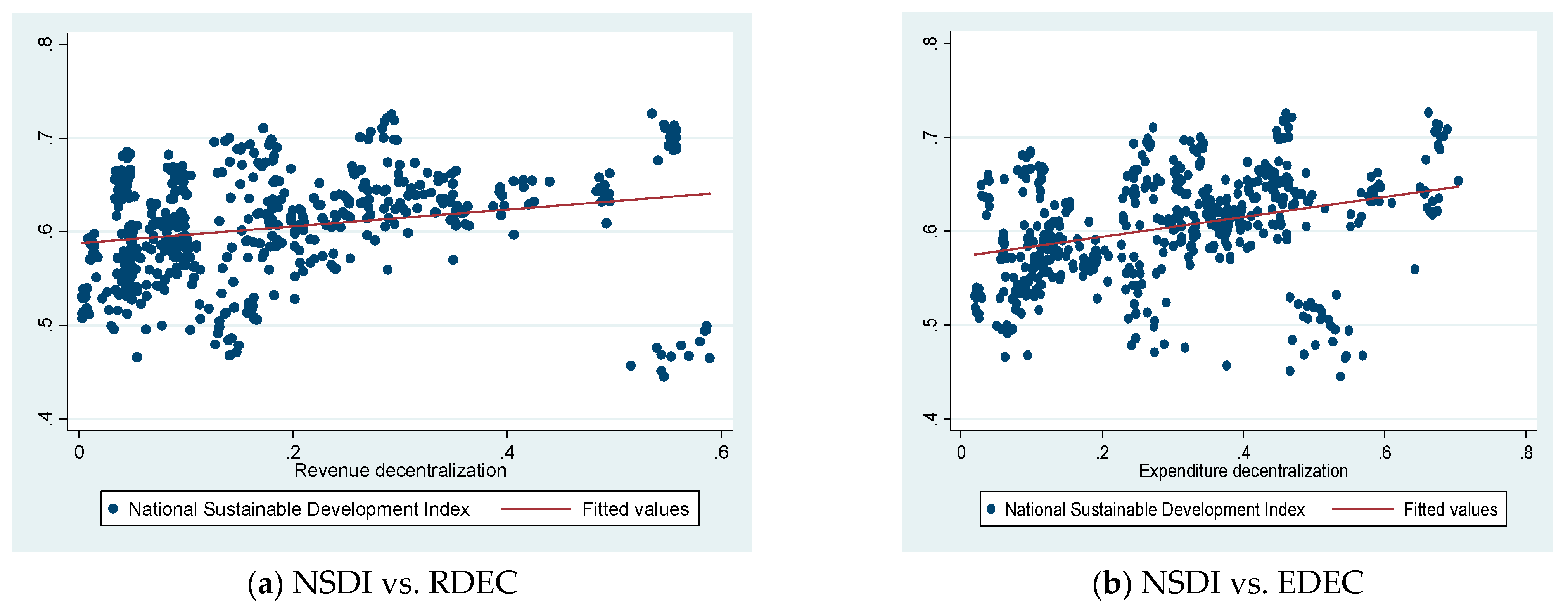
A preliminary pairwise correlation analysis reveals a positive correlation between revenue decentralization and each of NSDI, ECODI, and ERDI, and a negative but very weak correlation between RDEC and SOCDI. Expenditure decentralization is positively correlated with all the Sustainable Development Indices. NSDI is positively correlated with each of ECODI, ERDI, and SOCDI. ECODI and SOCDI are positively correlated, while each of them is negatively correlated with ERDI. This confirms the trade-off between the economic and the social dimensions on one hand, and the energy and resource dimension on the other hand in the sustainable development theory. Regarding the correlation between the NSDI and the control variables, all except the correlation with physical capital are appropriately signed based on a priori expectations. The correlation between NSDI and physical capital is also very weak. The result of the pairwise correlation is shown in

Table 6. Pairwise correlation result.

	RDEC	EDEC	NSDI	ECODI	ERDI	SOCDI
RDEC	1
EDEC	0.8221	1
NSDI	0.2286	0.3263	1
ECODI	0.2743	0.3861	0.6823	1
ERDI	0.1863	0.1787	0.5923	−0.0791	1
SOCDI	−0.0194	0.1014	0.7053	0.6792	−0.0632	1
GOVSIZE	−0.0256	0.1424	0.3263	0.4301	−0.1535	0.5334
HUMANCAP	−0.0167	0.1994	0.4877	0.5812	−0.1272	0.7081
TRADEOP	0.2022	0.2447	0.2241	0.3357	−0.0024	0.1829
PHYCAP	−0.0752	−0.0298	−0.0802	−0.1063	−0.0832	0.0414
GSAVE	−0.1192	−0.0637	0.2541	0.25	0.0463	0.2573
UNEMPR	−0.0944	−0.0352	−0.1758	−0.1334	−0.1207	−0.0881
POPRATE	0.1385	0.0557	−0.1254	0.0334	−0.0285	−0.2625
ENERUSE	0.4171	0.5578	0.5312	0.7116	−0.1083	0.6564
ENERINT	0.1442	0.243	−0.2016	−0.2551	0.0277	−0.2437
NRDEPEND	−0.0014	0.0023	−0.2578	−0.2133	0.0281	−0.4047
NRDEPLET	−0.0505	−0.0404	−0.2541	−0.18	−0.0236	−0.3537
QOG	0.1599	0.2233	0.5646	0.7499	−0.154	0.759
INCDISTR	−0.152	−0.1318	−0.4399	−0.3532	−0.0742	−0.5268

below. Moreover, Figure 1 shows the scatter plots and fitted lines of the various sustainable development indices against the different measures of fiscal federalism. It gives a first impression of the relationships between the sustainable development indices and the measures of fiscal federalism. The relationship between each of NSDI, ECODI, and ERDI, and each of RDEC and EDEC is positive. SOCDI has a negative relationship with RDEC and a positive relationship with EDEC. However, the exact relationship between fiscal federalism and sustainable development still has to be investigated empirically to account for confounding factors.

5.3. Results of Regression Analysis

The results of the various estimations performed in this study are presented in

Table A3. Regression results for RDEC on NSDI.

	Pooled OLS	FE	RE	DGMM_1	DGMM_2	SGMM_1	SGMM_2
L.NSDI	0.9655821 ***	0.322172 ***	0.965582 ***	0.029600	−0.123915	0.956179 ***	0.724836 ***
	(−0.009651)	(−0.037114)	(−0.009651)	(−0.106400)	(−0.098512)	(−0.012615)	(−0.165457)
RDEC	0.000815	0.051689 ***	0.000815	0.096808 *	0.072170	0.001674	−0.202004 *
	(0.003297)	(0.017093)	(0.003297)	(0.055154)	(0.108285)	(0.004005)	(0.100951)
GOVSIZE	−0.000187	−0.00072 ***	−0.000187	−0.001411 *	−0.000635	−0.000203	−0.001298 **
	(0.000153)	(0.000315)	(0.000153)	(0.000784)	(0.000664)	(0.000149)	(0.000503)
HUMANCAP	0.0000496 *	0.000182 ***	0.00005 *	−0.000052	−0.000156	0.000058	−0.000297
	(0.000029)	(0.000050)	(0.000029)	(0.000109)	(0.000142)	(0.000027)	(0.000237)
TRADEOP	−0.000005	−0.000073	−0.000005	0.000033	0.000495	−0.000008 **	0.000361 *
	(0.000058)	(0.000116)	(0.000058)	(0.000260)	(0.000371)	(0.000043)	(0.000196)
PHYCAP	−0.007826	−0.0364 ***	−0.007826	−0.010131	0.067798	−0.009582	0.051271
	(0.008915)	(0.012919)	(0.008915)	(0.036465)	(0.053852)	(0.014647)	(0.045830)
GSAVE	0.000076	0.000091	0.000076	0.000192	0.000037	0.000096	−0.000800
	(0.000070)	(0.000108)	(0.000070)	(0.000167)	(0.000143)	(0.000078)	(0.000581)
UNEMPR	−0.000014	−0.000278	−0.000014	−0.000170	−0.000032	−0.000021	0.000008
	(0.000079)	(0.000183)	(0.000079)	(0.000232)	(0.000196)	(0.000046)	(0.000115)
POPRATE	−0.001434 **	−0.001783 *	−0.001434 **	0.000792	0.000774	−0.00155 ***	0.004155
	(0.000583)	(0.001077)	(0.000583)	(0.001269)	(0.001044)	(0.000490)	(0.003697)
ENERUSE	0.002021	0.008782 **	0.002021	0.017086 *	0.016002 ***	0.002166	0.040210 **
	(0.001388)	(0.004133)	(0.001388)	(0.009257)	(0.005249)	(0.001418)	(0.016894)
ENERINT	−0.000217	−0.00126 ***	−0.000217	−0.00401 ***	−0.00404 **	−0.000269	−0.003828 **
	(0.000324)	(0.000702)	(0.000324)	(0.001337)	(0.001534)	(0.000235)	(0.001489)
NRDEPEND	0.0005798 **	0.00106 ***	0.00058 **	0.001455 **	0.000637 *	0.000641 **	0.002013 **
	(0.000267)	(0.000352)	(0.000267)	(0.000549)	(0.000480)	(0.000282)	(0.000803)
NRDEPLET	−0.001088 **	−0.001451 *	−0.001088 **	−0.002504 **	−0.001321	−0.001198 **	−0.00573 ***
	(0.000436)	(0.000624)	(0.000436)	(0.001074)	(0.000742)	(0.000468)	(0.002070)
QOG	−0.000083	−0.000680	−0.000083	−0.000379	−0.000400	−0.000072	−0.001334 *
	(0.000149)	(0.000568)	(0.000149)	(0.001157)	(0.000682)	(0.000106)	(0.000718)
INCDISTR	−0.000048	0.000129	−0.000048	0.000820	0.000207	−0.000060	−0.002128 **
	(0.000302)	(0.000687)	(0.000302)	(0.001580)	(0.000828)	(0.000189)	(0.000912)
Time dummy	Yes	Yes	Yes	Yes	Yes	Yes	Yes
Robust Hausman		364.71 ***
AR(1)				[0.020]	[0.280]	[0.001]	[0.001]
AR(2)				[0.399]	[0.206]	[0.247]	[0.134]
Hansenp				[1.000]	[1.000]	[1.000]	[1.000]
Diff-Hansen						[1.000]	[1.000]
Observations	480	480	480	440	440	480	480
No. of countries	40	40	40	40	40	40	40

The dependent variable is NSDI. *, ** and *** denote statistical significance at 10%, 5% and 1% respectively. Standard errors are in parenthesis and p-values in brackets. All estimates use robust standard errors. DGMM_1, DGMM_2, SGMM_1, and SGMM_2 are the one-step difference GMM, two-step difference GMM, one-step system GMM, and two-step system GMM, respectively. In the GMM estimations, NSDI, revenue decentralization, and physical capital are treated as endogenous, and the other regressors as exogenous. The value reported for the Hansen J- test (Hansenp) are the p-values for null hypothesis of the overidentification restrictions. Similarly, the values reported for the Difference-in-Hansen (Diff-Hansen) test are the p-values of the null hypothesis of the additional moment restrictions necessary for the system GMM given in Equation (9). Moreover, the values reported for the AR(1) and AR(2) are, respectively, the p-values of the first order and second order autocorrelated disturbances in the Arellano-Bond test for autocorrelation in the first differences error. The decision is based on both SGMM_1 and SGMM_2.

,

Table A4. Regression results for EDEC on NSDI.

	Pooled OLS	FE	RE	DGMM_1	DGMM_2	SGMM_1	SGMM_2
L.NSDI	0.965111 ***	0.321974 ***	0.965111 ***	0.063932	−0.103983	0.946364 ***	0.427128 **
	(0.009753)	(0.037409)	(0.009753)	(0.095101)	(0.112199)	(0.013813)	(0.201518)
EDEC	0.001145	0.017149	0.001145	0.059335 *	0.048599	−0.000319	0.002365
	(0.002763)	(0.010521)	(0.002763)	(0.026999)	(0.037113)	(0.003854)	(0.049532)
GOVSIZE	−0.000187	−0.000670 **	−0.000187	−0.001514 *	−0.000260	−0.000291 *	−0.000325
	(0.000152)	(0.000318)	(0.000152)	(0.000755)	(0.000977)	(0.000150)	(0.000409)
HUMANCAP	0.000049 *	0.000196 ***	0.000049 *	0.000009	−0.000043	0.000069 **	0.000262 **
	(0.000028)	(0.000050)	(0.000028)	(0.000122)	(0.000151)	(0.000030)	(0.000107)
TRADEOP	−0.000006	−0.000059	−0.000006	−0.000153	0.000418	−0.000028	0.000373
	(0.000058)	(0.000118)	(0.000058)	(0.000273)	(0.000501)	(0.000046)	(0.000304)
PHYCAP	−0.007869	−0.035203 ***	−0.007869	−0.029101	0.059577	−0.018682	0.061937
	(0.008876)	(0.013043)	(0.008876)	(0.035398)	(0.079911)	(0.013429)	(0.086578)
GSAVE	0.000077	0.000073	0.000077	0.000146	−0.000093	0.000124	0.000517
	(0.000070)	(0.000109)	(0.000070)	(0.000164)	(0.000188)	(0.000087)	(0.000377)
UNEMPR	−0.000015	−0.000200	−0.000015	−0.000251	−0.000203	−0.000032	−0.000248
	(0.000079)	(0.000184)	(0.000079)	(0.000271)	(0.000252)	(0.000051)	(0.000153)
POPRATE	−0.001442 **	−0.001324	−0.001442 **	0.000933	0.000741	−0.00166 ***	−0.004427 *
	(0.000579)	(0.001070)	(0.000579)	(0.001552)	(0.001195)	(0.000585)	(0.002209)
ENERUSE	0.001934	0.007338 *	0.001934	0.010066 *	0.008357	0.003025 **	0.013354
	(0.001382)	(0.004160)	(0.001382)	(0.008934)	(0.005370)	(0.001227)	(0.009643)
ENERINT	−0.000222	−0.001099	−0.000222	−0.00329 ***	−0.00364 ***	−0.000370	−0.00311 ***
	(0.000323)	(0.000726)	(0.000323)	(0.001150)	(0.001327)	(0.000252)	(0.001050)
NRDEPEND	0.000581 **	0.001336 **	0.000581 **	0.001687 **	0.001124 **	0.000777 ***	0.002586 ***
	(0.000267)	(0.000354)	(0.000267)	(0.000701)	(0.000526)	(0.000284)	(0.000867)
NRDEPLET	−0.001089 **	−0.001904 **	−0.001089 **	−0.002734 **	−0.00218 ***	−0.00143 ***	−0.00591 ***
	(0.000434)	(0.000617)	(0.000434)	(0.001266)	(0.000696)	(0.000471)	(0.001849)
QOG	−0.000077	−0.000522	−0.000077	0.000751	0.000786	−0.000093	0.000425
	(0.000150)	(0.000572)	(0.000150)	(0.000979)	(0.000702)	(0.000113)	(0.000492)
INCDISTR	−0.000059	−0.000063	−0.000059	0.000105	0.000205	−0.000075	−0.001522 **
	(0.000302)	(0.000699)	(0.000302)	(0.001051)	(0.000614)	(0.000224)	(0.000608)
Time dummy	Yes	Yes	Yes	Yes	Yes	Yes	Yes
Robust Hausman		351.68 ***
AR(1)				[0.008]	[0.288]	[0.001]	[0.076]
AR(2)				[0.500]	[0.166]	[0.283]	[0.175]
Diff-Hansenp				[1.000]	[1.000]	[1.000]	[1.000]
Hansen						[1.000]	[1.000]
Observations	480	480	480	440	440	480	480
No. of countries	40	40	40	40	40	40	40

The dependent variable is NSDI. *, ** and *** denote statistical significance at 10%, 5% and 1% respectively. Standard errors are in parenthesis and p-values in brackets. All estimates use robust standard errors. DGMM_1, DGMM_2, SGMM_1, and SGMM_2 are the one-step difference GMM, two-step difference GMM, one-step system GMM, and two-step system GMM, respectively. In the GMM estimations, NSDI, expenditure decentralization, and physical capital are treated as endogenous, and the other regressors as exogenous. The value reported for the Hansen J- test (Hansenp) are the p-values for null hypothesis of the overidentification restrictions. Similarly, the values reported for the Difference-in-Hansen (Diff-Hansen) test are the p-values of the null hypothesis of the additional moment restrictions necessary for the system GMM given in Equation (9). Moreover, the values reported for the AR(1) and AR(2) are, respectively, the p-values of the first order and second order autocorrelated disturbances in the Arellano-Bond test for autocorrelation in the first differences error. The decision is based on both SGMM_1 and SGMM_2.

,

Table A5. Regression results for RDEC on ECODI.

	Pooled OLS	FE	RE	DGMM_1	DGMM_2	SGMM_1	SGMM_2
L.ECODI	0.937646 ***	0.469099 ***	0.937646 ***	0.366774 ***	0.154428 *	0.924119 ***	0.944140 ***
	(0.016132)	(0.038814)	(0.016132)	(0.076735)	(0.090478)	(0.017747)	(0.091166)
RDEC	0.013281 *	0.043096	0.013281 *	0.292219 *	0.417621 **	0.024441 **	0.061138
	(0.006984)	(0.043931)	(0.006984)	(0.149027)	(0.164638)	(0.010630)	(0.142275)
GOVSIZE	0.000181	−0.0025 ***	0.000181	−0.00619 ***	−0.00732 ***	0.000086	−0.000746
	(0.000311)	(0.000836)	(0.000311)	(0.001788)	(0.001145)	(0.000292)	(0.001734)
HUMANCAP	0.000130 *	0.000124	0.000130 *	0.000124	−0.000361	0.000187 **	0.000277
	(0.000068)	(0.000126)	(0.000068)	(0.000358)	(0.000285)	(0.000072)	(0.000259)
TRADEOP	−0.000101	−0.000333	−0.000101	−0.000348	−0.000530	−0.000155	−0.000492
	(0.000104)	(0.000261)	(0.000104)	(0.000527)	(0.000437)	(0.000158)	(0.000860)
PHYCAP	−0.009729	−0.035140	−0.009729	−0.026095	−0.018932	−0.032026	−0.103931
	(0.018407)	(0.032433)	(0.018407)	(0.079359)	(0.063946)	(0.024340)	(0.123524)
GSAVE	0.000224	0.000671 **	0.000224	0.000997 **	0.001047 ***	0.000336 **	0.000572
	(0.000150)	(0.000279)	(0.000150)	(0.000472)	(0.000224)	(0.000155)	(0.000973)
UNEMPR	−0.000037	−0.000284	−0.000037	0.000343	−0.000274	−0.000043	0.000007
	(0.000173)	(0.000467)	(0.000173)	(0.000549)	(0.000528)	(0.000118)	(0.000519)
Time dummy	Yes	Yes	Yes	Yes	Yes	Yes	Yes
Robust Hausman		199.43 ***
AR(1)				[0.000]	[0.006]	[0.000]	[0.000]
AR(2)				[0.176]	[0.194]	[0.070]	[0.095]
Hansenp				[1.000]	[1.000]	[1.000]	[1.000]
Diff-Hansen						[1.000]	[1.000]
Observations	480	480	480	440	440	480	480
No. of countries	40	40	40	40	40	40	40

The dependent variable is ECODI. *, ** and *** denote statistical significance at 10%, 5% and 1% respectively. Standard errors are in parenthesis and p-values in brackets. All estimates use robust standard errors. DGMM_1, DGMM_2, SGMM_1, and SGMM_2 are the one-step difference GMM, two-step difference GMM, one-step system GMM, and two-step system GMM, respectively. In the GMM estimations, ECODI, revenue decentralization, and physical capital are treated as endogenous, and the other regressors as exogenous. The value reported for the Hansen J- test (Hansenp) are the p-values for null hypothesis of the overidentification restrictions. Similarly, the values reported for the Difference-in-Hansen (Diff-Hansen) test are the p-values of the null hypothesis of the additional moment restrictions necessary for the system GMM given in Equation (9). Moreover, the values reported for the AR(1) and AR(2) are, respectively, the p-values of the first order and second order autocorrelated disturbances in the Arellano-Bond test for autocorrelation in the first differences error. The decision is based on the SGMM_1.

,

Table A6. Regression results for EDEC on ECODI.

	Pooled OLS	FE	RE	DGMM_1	DGMM_2	SGMM_1	SGMM_2
L.ECODI	0.937603 ***	0.465944 ***	0.937603 ***	0.381886 ***	0.215060 **	0.914926 ***	0.823596 ***
	(0.015859)	(0.038644)	(0.015859)	(0.072046)	(0.100945)	(0.018316)	(0.101793)
EDEC	0.012226 **	0.057995 **	0.012226 **	0.139287 ***	0.171085 ***	0.029429 **	0.059710
	(0.005766)	(0.025749)	(0.005766)	(0.050224)	(0.043942)	(0.011376)	(0.054778)
GOVSIZE	0.000136	−0.00259 ***	0.000136	−0.00511 ***	−0.00436 ***	−0.000100	0.000702
	(0.000312)	(0.000829)	(0.000312)	(0.001235)	(0.001151)	(0.000339)	(0.001101)
HUMANCAP	0.000113 *	0.000139	0.000113 *	0.000269	0.000104	0.000188 **	0.000233
	(0.000066)	(0.000126)	(0.000066)	(0.000370)	(0.000215)	(0.000081)	(0.000161)
TRADEOP	−0.000114	−0.000355	−0.000114	−0.000762	−0.000527	−0.000228 *	0.000010
	(0.000104)	(0.000260)	(0.000104)	(0.000614)	(0.000602)	(0.000171)	(0.000455)
PHYCAP	−0.012355	−0.030241	−0.012355	−0.056644	−0.004354	−0.055892	0.034543
	(0.018497)	(0.032201)	(0.018497)	(0.079229)	(0.093066)	(0.030486)	(0.108089)
GSAVE	0.000223	0.000667 **	0.000223	0.000993 *	0.001046	0.000412 **	0.000401
	(0.000148)	(0.000277)	(0.000148)	(0.000500)	(0.000265)	(0.000190)	(0.000433)
UNEMPR	−0.000060	−0.000120	−0.000060	0.000055	−0.000178	−0.000106	−0.000206
	(0.000172)	(0.000469)	(0.000172)	(0.000572)	(0.000633)	(0.000142)	(0.000193)
Time dummy	Yes	Yes	Yes	Yes	Yes	Yes	Yes
Robust Hausman		204.58 ***
AR(1)				[0.000]	[0.012]	[0.000]	[0.000]
AR(2)				[0.134]	[0.125]	[0.079]	[0.072]
Hansenp				[1.000]	[1.000]	[1.000]	[1.000]
Diff-Hansen						[1.000]	[1.000]
Observations	480	480	480	440	440	480	480
No. of countries	40	40	40	40	40	40	40

The dependent variable is ECODI. *, ** and *** denote statistical significance at 10%, 5% and 1% respectively. Standard errors are in parenthesis and p-values in brackets. All estimates use robust standard errors. DGMM_1, DGMM_2, SGMM_1, and SGMM_2 are the one-step difference GMM, two-step difference GMM, one-step system GMM, and two-step system GMM, respectively. In the GMM estimations, ECODI, expenditure decentralization, and physical capital are treated as endogenous, and the other regressors as exogenous. The value reported for the Hansen J- test (Hansenp) are the p-values for null hypothesis of the overidentification restrictions. Similarly, the values reported for the Difference-in-Hansen (Diff-Hansen) test are the p-values of the null hypothesis of the additional moment restrictions necessary for the system GMM given in Equation (9). Moreover, the values reported for the AR(1) and AR(2) are, respectively, the p-values of the first order and second order autocorrelated disturbances in the Arellano-Bond test for autocorrelation in the first differences error. The decision is based on the SGMM_1.

,

Table A7. Regression results for RDEC on ERDI.

	Pooled OLS	FE	RE	DGMM_1	DGMM_2	SGMM_1	SGMM_2
L.ERDI	0.982010 ***	0.358617 ***	0.96997 ***	0.18863 ***	0.19748 ***	0.95808 ***	0.77081 ***
	(0.008003)	(0.029644)	(0.009628)	(0.065543)	(0.035018)	(0.016068)	(0.091809)
RDEC	0.001674	0.070226 ***	0.003569	0.090171	0.050766	−0.000109	0.030884
	(0.004328)	(0.022528)	(0.005235)	(0.091811)	(0.033155)	(0.006986)	(0.026291)
ENERUSE	0.001921 **	−0.005450	0.001696 *	0.004137	0.004800	0.001803 **	−0.002519
	(0.000825)	(0.005243)	(0.001000)	(0.012963)	(0.004426)	(0.000806)	(0.002363)
ENERINT	0.000618 **	−0.002050 **	0.000626 *	−0.0066 ***	−0.0050 ***	0.000580 *	0.000676 **
	(0.000287)	(0.000945)	(0.000341)	(0.002152)	(0.001513)	(0.000340)	(0.000259)
NRDEPEND	−0.000303	0.001201 ***	−0.000217	0.000750	0.000603 **	−0.000054	0.000933
	(0.000345)	(0.000456)	(0.000389)	(0.001246)	(0.000241)	(0.000643)	(0.000922)
NRDEPLET	0.000379	−0.001057	0.000225	−0.000567	−0.000491	−0.000031	−0.001563
	(0.000566)	(0.000734)	(0.000638)	(0.002212)	(0.000362)	(0.000971)	(0.001526)
Time dummy	Yes	Yes	Yes	Yes	Yes	Yes	Yes
Robust Hausman		513.14 ***
AR(1)				[0.047]	[0.026]	[0.010]	[0.015]
AR(2)				[0.684]	[0.717]	[0.505]	[0.527]
Hansenp				[1.000]	[1.000]	[1.000]	[1.000]
Diff-Hansen						[1.000]	[1.000]
Observations	480	480	480	440	440	480	480
No. of countries	40	40	40	40	40	40	40

The dependent variable is ERDI. *, ** and *** denote statistical significance at 10%, 5% and 1% respectively. Standard errors are in parenthesis and p-values in brackets. All estimates use robust standard errors. DGMM_1, DGMM_2, SGMM_1, and SGMM_2 are the one-step difference GMM, two-step difference GMM, one-step system GMM, and two-step system GMM, respectively. In the GMM estimations, ERDI and revenue decentralization are treated as endogenous, and the other regressors as exogenous. The value reported for the Hansen J- test (Hansenp) are the p-values for null hypothesis of the overidentification restrictions. Similarly, the values reported for the Difference-in-Hansen (Diff-Hansen) test are the p-values of the null hypothesis of the additional moment restrictions necessary for the system GMM given in Equation (9). Moreover, the values reported for the AR(1) and AR(2) are, respectively, the p-values of the first order and second order autocorrelated disturbances in the Arellano-Bond test for autocorrelation in the first differences error. The decision is based on both SGMM_1 and SGMM_2.

,

Table A8. Regression results for EDEC on ERDI.

	Pooled OLS	FE	RE	DGMM_1	DGMM_2	SGMM_1	SGMM_2
L.ERDI	0.982337 ***	0.355802 ***	0.971112 ***	0.139630 **	0.16414 ***	0.97217 ***	0.7028 ***
	(0.008107)	(0.029947)	(0.009647)	(0.061539)	(0.024893)	(0.014428)	(0.085740)
EDEC	0.000632	0.011279	0.001950	0.051991	0.04319 ***	−0.009746	0.010885
	(0.003943)	(0.013830)	(0.004681)	(0.058608)	(0.015440)	(0.010246)	(0.020250)
ENERUSE	0.001981 **	−0.005829	0.001748	0.001191	−0.002147	0.003151 **	−0.002188
	(0.000899)	(0.005324)	(0.001075)	(0.012097)	(0.003555)	(0.001458)	(0.002887)
ENERINT	0.000609 **	−0.002079 **	0.000606 *	−0.005312 *	−0.0057 ***	0.000647 **	0.000137
	(0.000287)	(0.000970)	(0.000339)	(0.001970)	(0.001289)	(0.000307)	(0.000219)
NRDEPEND	−0.000286	0.001530 ***	−0.000193	0.000282	0.000392	−0.000075	0.0021 ***
	(0.000342)	(0.000459)	(0.000383)	(0.001354)	(0.000269)	(0.000613)	(0.000728)
NRDEPLET	0.000351	−0.001611 **	0.000186	−0.000213	−0.000254	0.000011	−0.0037 ***
	(0.000560)	(0.000729)	(0.000628)	(0.002447)	(0.000525)	(0.000910)	(0.001207)
Time dummy	Yes	Yes	Yes	Yes	Yes	Yes	Yes
Robust Hausman		491.04 ***
AR(1)				[0.061]	[0.035]	[0.010]	[0.016]
AR(2)				[0.478]	[0.538]	[0.493]	[0.449]
Hansenp				[1.000]	[1.000]	[1.000]	[1.000]
Diff-Hansen						[1.000]	[1.000]
Observations	480	480	480	440	440	480	480
No. of countries	40	40	40	40	40	40	40

The dependent variable is ERDI. *, ** and *** denote statistical significance at 10%, 5% and 1% respectively. Standard errors are in parenthesis and p-values in brackets. All estimates use robust standard errors. DGMM_1, DGMM_2, SGMM_1, and SGMM_2 are the one-step difference GMM, two-step difference GMM, one-step system GMM, and two-step system GMM, respectively. In the GMM estimations, ERDI and expenditure decentralization are treated as endogenous, and the other regressors as exogenous. The value reported for the Hansen J- test (Hansenp) are the p-values for null hypothesis of the overidentification restrictions. Similarly, the values reported for the Difference-in-Hansen (Diff-Hansen) test are the p-values of the null hypothesis of the additional moment restrictions necessary for the system GMM given in Equation (9). Moreover, the values reported for the AR(1) and AR(2) are, respectively, the p-values of the first order and second order autocorrelated disturbances in the Arellano-Bond test for autocorrelation in the first differences error. The decision is based on both SGMM_1 and SGMM_2.

,

Table A9. Regression results for RDEC on SOCDI.

	Pooled OLS	FE	RE	DGMM_1	DGMM_2	SGMM_1	SGMM_2
L.SOCDI	0.992378 ***	0.900734 ***	0.98949 ***	0.89985 ***	0.88739 ***	0.9937 ***	0.9768 ***
	(0.004072)	(0.020565)	(0.004991)	(0.035279)	(0.056027)	(0.006591)	(0.030013)
RDEC	−0.002671	−0.009034	−0.003102	−0.002590	−0.000645	−0.005748 *	−0.005382
	(0.001821)	(0.013822)	(0.002255)	(0.026723)	(0.019345)	(0.003126)	(0.014423)
POPRATE	0.001016 ***	−0.000511	0.000912 *	0.000812	0.000601	0.00114 **	0.000908
	(0.000304)	(0.000813)	(0.000364)	(0.000964)	(0.000616)	(0.000425)	(0.001043)
QOG	−0.000141 *	0.000532	−0.000100	0.001447 *	0.000832 *	−0.000150	0.000092
	(0.000077)	(0.000461)	(0.000095)	(0.000795)	(0.000493)	(0.000128)	(0.000376)
INCDISTR	0.000176	−0.001508 *	0.000097	−0.002017	−0.00193 **	0.000149	−0.000042
	(0.000177)	(0.000582)	(0.000215)	(0.001243)	(0.000830)	(0.000152)	(0.000348)
Time dummy	Yes	Yes	Yes	Yes	Yes	Yes	Yes
Robust Hausman		28.65 **
AR(1)				[0.001]	[0.001]	[0.000]	[0.001]
AR(2)				[0.323]	[0.327]	[0.287]	[0.302]
Hansenp				[1.000]	[1.000]	[1.000]	[1.000]
Diff-Hansen						[1.000]	[1.000]
Observations	480	480	480	440	440	480	480
No. of countries	40	40	40	40	40	40	40

The dependent variable is SOCDI. *, ** and *** denote statistical significance at 10%, 5% and 1% respectively. Standard errors are in parenthesis and p-values in brackets. All estimates use robust standard errors. DGMM_1, DGMM_2, SGMM_1, and SGMM_2 are the one-step difference GMM, two-step difference GMM, one-step system GMM, and two-step system GMM, respectively. In the GMM estimations, SOCDI and revenue decentralization are treated as endogenous, and the other regressors as exogenous. The value reported for the Hansen J- test (Hansenp) are the p-values for null hypothesis of the overidentification restrictions. Similarly, the values reported for the Difference-in-Hansen (Diff-Hansen) test are the p-values of the null hypothesis of the additional moment restrictions necessary for the system GMM given in Equation (9). Moreover, the values reported for the AR(1) and AR(2) are, respectively, the p-values of the first order and second order autocorrelated disturbances in the Arellano-Bond test for autocorrelation in the first differences error. The decision is based on SGMM_2.

,

Table A10. Regression results for EDEC on SOCDI.

	Pooled OLS	FE	RE	DGMM_1	DGMM_2	SGMM_1	SGMM_2
L.SOCDI	0.993306 ***	0.900022 ***	0.9905 ***	0.89467 ***	0.8932 ***	0.99461 ***	0.99177 ***
	(0.003968)	(0.020522)	(0.004883)	(0.041789)	(0.040417)	(0.006071)	(0.027716)
EDEC	−0.001797	−0.007507	−0.002098	0.006231	0.009555	−0.004036	−0.008462
	(0.001453)	(0.008111)	(0.001801)	(0.014411)	(0.009799)	(0.002818)	(0.008151)
POPRATE	0.000984 ***	−0.000483	0.00088 **	−0.000262	−0.000458	0.001054 **	0.001218 **
	(0.000303)	(0.000812)	(0.000364)	(0.000976)	(0.000580)	(0.000421)	(0.000488)
QOG	−0.000150 **	0.000506	−0.000110	0.001414 *	0.001205 *	−0.000154	−0.000105
	(0.000076)	(0.000460)	(0.000094)	(0.000740)	(0.000598)	(0.000127)	(0.000195)
INCDISTR	0.000213	−0.001458 **	0.000136	−0.00197 **	−0.0022 ***	0.00021	0.000246
	(0.000173)	(0.000583)	(0.000211)	(0.000935)	(0.000413)	(0.000146)	(0.000243)
Time dummy	Yes	Yes	Yes	Yes	Yes	Yes	Yes
Robust Hausman		29.42 **
AR(1)				[0.001]	[0.001]	[0.000]	[0.000]
AR(2)				[0.304]	[0.311]	[0.288]	[0.307]
Hansenp				[1.000]	[1.000]	[1.000]	[1.000]
Diff-Hansen						[1.000]	[1.000]
Observations	480	480	480	440	440	480	480
No. of countries	40	40	40	40	40	40	40

The dependent variable is SOCDI. *, ** and *** denote statistical significance at 10%, 5% and 1% respectively. Standard errors are in parenthesis and p-values in brackets. All estimates use robust standard errors. DGMM_1, DGMM_2, SGMM_1, and SGMM_2 are the one-step difference GMM, two-step difference GMM, one-step system GMM, and two-step system GMM, respectively. In the GMM estimations, SOCDI and expenditure decentralization are treated as endogenous, and the other regressors as exogenous. The value reported for the Hansen J- test (Hansenp) are the p-values for null hypothesis of the overidentification restrictions. Similarly, the values reported for the Difference-in-Hansen (Diff-Hansen) test are the p-values of the null hypothesis of the additional moment restrictions necessary for the system GMM given in Equation (9). Moreover, the values reported for the AR(1) and AR(2) are, respectively, the p-values of the first order and second order autocorrelated disturbances in the Arellano-Bond test for autocorrelation in the first differences error. The decision is based on SGMM_2.

,

Table A11. Regression results for RDEC on NSDI with federation interaction variable.

	Pooled OLS	FE	RE	DGMM_1	DGMM_2	SGMM_1	SGMM_2
L.NSDI	0.965511 ***	0.324126 ***	0.96551 ***	0.140835 *	−0.160793	0.964 ***	0.451701 **
	(0.009694)	(0.037173)	(0.009694)	(0.081829)	(0.174113)	(0.009114)	(0.205763)
RDEC	0.001239	0.059676 ***	0.001239	0.067337	0.069344	0.001077	−0.098444
	(0.005769)	(0.019009)	(0.005769)	(0.051351)	(0.098479)	(0.005129)	(0.122921)
GOVSIZE	−0.000189	−0.000682 **	−0.000189	−0.001189 *	0.000477	−0.000237 *	−0.000502
	(0.000154)	(0.000318)	(0.000154)	(0.000649)	(0.000702)	(0.000121)	(0.000503)
HUMANCAP	0.000049 *	0.000184 **	0.000049 *	0.000013	−0.000166	0.000055 **	−0.00036 **
	(0.000029)	(0.00005)	(0.000029)	(0.000102)	(0.000114)	(0.000024)	(0.000169)
TRADEOP	−0.000006	−0.000061	−0.000006	0.000102	0.001256 **	−0.000023	0.000808 **
	(0.000059)	(0.000117)	(0.000059)	(0.000243)	(0.000488)	(0.000037)	(0.000329)
PHYCAP	−0.008081	−0.03589 ***	−0.008081	−0.012138	0.165893 **	−0.014209	0.190064 **
	(0.009367)	(0.012932)	(0.009367)	(0.033472)	(0.076109)	(0.011204)	(0.092465)
GSAVE	0.000077	0.000089	0.000077	0.000091	−0.000306	0.000093	−0.000815 *
	(0.000071)	(0.000108)	(0.000071)	(0.000159)	(0.000213)	(0.000069)	(0.000478)
UNEMPR	−0.000013	−0.000292	−0.000013	−0.000369 *	0.000006	−0.000017	0.000241 *
	(0.000079)	(0.000183)	(0.000079)	(0.000214)	(0.000267)	(0.000044)	(0.000132)
POPRATE	−0.001427 **	−0.001809 *	−0.00143 **	−0.000168	0.000895	−0.0015 ***	0.005782 **
	(0.000588)	(0.001078)	(0.000588)	(0.001172)	(0.001094)	(0.000472)	(0.002496)
ENERUSE	0.002012	0.0085 **	0.002012	0.013452 *	0.01528 ***	0.002301 **	0.038053 **
	(0.001394)	(0.004144)	(0.001394)	(0.006896)	(0.005274)	(0.001118)	(0.015845)
ENERINT	−0.000216	−0.001268 *	−0.000216	−0.00259 **	0.00034 ***	−0.000245	−0.0046 ***
	(0.000325)	(0.000702)	(0.000325)	(0.001058)	(0.000505)	(0.000214)	(0.001595)
NRDEPEND	0.000582 **	0.001056 ***	0.000582 **	0.00152 ***	−0.001381	0.00065 ***	0.00206 ***
	(0.000268)	(0.000352)	(0.000268)	(0.000428)	(0.000836)	(0.000225)	(0.000697)
NRDEPLET	−0.001089 **	−0.001441 **	−0.00109 **	−0.0027 ***	−0.000163	−0.0012 ***	−0.0066 ***
	(0.000437)	(0.000624)	(0.000437)	(0.000777)	(0.000834)	(0.000365)	(0.002037)
QOG	−0.000080	−0.000749	−0.000080	−0.000057	−0.000163	−0.000088	−0.000151
	(0.000153)	(0.000573)	(0.000153)	(0.000984)	(0.000834)	(0.000095)	(0.000908)
INCDISTR	−0.000054	0.000166	−0.000054	0.001025	0.000169	−0.000055	−0.0044 ***
	(0.00031)	(0.000688)	(0.00031)	(0.001322)	(0.001028)	(0.000182)	(0.001385)
IRDEC	−0.000422	−0.039575	−0.000422	0.008712	−0.078175	−0.000789	−0.096491
	(0.004723)	(0.041183)	(0.004723)	(0.097245)	(0.149207)	(0.004003)	(0.064056)
Time dummy	Yes	Yes	Yes	Yes	Yes	Yes	Yes
Robust Hausman		368.74 ***
AR(1)				[0.004]	[0.707]	[0.001]	[0.086]
AR(2)				[0.407]	[0.169]	[0.259]	[0.003]
Hansenp				[1.000]	[1.000]	[1.000]	[1.000]
Diff-Hansen						[1.000]	[1.000]
Observations	480	480	480	440	440	480	480
No. of countries	40	40	40	40	40	40	40

The dependent variable is NSDI. *, ** and *** denote statistical significance at 10%, 5% and 1% respectively. Standard errors are in parenthesis and p-values in brackets. All estimates use robust standard errors. DGMM_1, DGMM_2, SGMM_1, and SGMM_2 are the one-step difference GMM, two-step difference GMM, one-step system GMM, and two-step system GMM, respectively. In the GMM estimations, NSDI, revenue decentralization, and human capital are treated as endogenous, and the other regressors as exogenous. The value reported for the Hansen J- test (Hansenp) are the p-values for null hypothesis of the overidentification restrictions. Similarly, the values reported for the Difference-in-Hansen (Diff-Hansen) test are the p-values of the null hypothesis of the additional moment restrictions necessary for the system GMM given in Equation (9). Moreover, the values reported for the AR(1) and AR(2) are, respectively, the p-values of the first order and second order autocorrelated disturbances in the Arellano-Bond test for autocorrelation in the first differences error. The decision is based on both SGMM_1 and SGMM_2.

,

Table A12. Regression results for EDEC on NSDI with federation interaction variable.

	Pooled OLS	FE	RE	DGMM_1	DGMM_2	SGMM_1	SGMM_2
L.NSDI	0.965114 ***	0.31463 ***	0.96511 ***	0.111443	−0.020354	0.96358 ***	0.386428 **
	(0.009763)	(0.038096)	(0.009763)	(0.077243)	(0.100195)	(0.009627)	(0.183723)
EDEC	0.000709	0.007918	0.000709	0.030625	0.0436	0.000898	0.242977 **
	(0.003486)	(0.013886)	(0.003486)	(0.029703)	(0.047263)	(0.002665)	(0.101304)
GOVSIZE	−0.000185	−0.00071 **	−0.000185	−0.001335 *	0.000222	−0.000229 *	−0.001103 *
	(0.000152)	(0.000321)	(0.000152)	(0.000722)	(0.000982)	(0.000116)	(0.00065)
HUMANCAP	0.000049 *	0.000194 ***	0.000049 *	0.000110	0.000025	0.000055 **	0.000005
	(0.000029)	(0.00005)	(0.000029)	(0.000104)	(0.000184)	(0.000025)	(0.000144)
TRADEOP	−0.000004	−0.000066	−0.000004	−0.000092	0.000551	−0.000021	−0.000756
	(0.000059)	(0.000118)	(0.000059)	(0.000248)	(0.000649)	(0.000038)	(0.000511)
PHYCAP	−0.007422	−0.03558 ***	−0.007422	−0.028626	0.079376	−0.013496	−0.140613
	(0.009146)	(0.013047)	(0.009146)	(0.032306)	(0.100744)	(0.010562)	(0.112509)
GSAVE	0.000077	0.000065	0.000077	0.000094	−0.000156	0.000094	0.000615
	(0.00007)	(0.000109)	(0.00007)	(0.000165)	(0.000256)	(0.000069)	(0.000402)
UNEMPR	−0.000015	−0.000192	−0.000015	−0.000227	0.000073	−0.000020	−0.000077
	(0.000079)	(0.000184)	(0.000079)	(0.000275)	(0.000268)	(0.000044)	(0.000176)
POPRATE	−0.001458 **	−0.001261	−0.00146 **	0.000636	0.000724	−0.0015 ***	0.000784
	(0.000585)	(0.001072)	(0.000585)	(0.00152)	(0.001189)	(0.000473)	(0.003199)
ENERUSE	0.001912	0.007877 *	0.001912	0.012918 *	0.008569	0.00216 **	0.027901
	(0.001388)	(0.004194)	(0.001388)	(0.007639)	(0.006075)	(0.000993)	(0.01984)
ENERINT	−0.000215	−0.001223 *	−0.000215	−0.00255 **	−0.00319 **	−0.000245	−0.00891 **
	(0.000325)	(0.000736)	(0.000325)	(0.001121)	(0.001199)	(0.000211)	(0.003333)
NRDEPEND	0.000576 **	0.001271 ***	0.000576 **	0.001558 **	0.000724	0.00064 ***	0.00558 ***
	(0.000268)	(0.00036)	(0.000268)	(0.00065)	(0.000675)	(0.000219)	(0.001595)
NRDEPLET	−0.001082 **	−0.00183 ***	−0.00108 **	−0.00277 **	−0.00178 **	−0.0012 ***	−0.0095 ***
	(0.000436)	(0.000621)	(0.000436)	(0.001121)	(0.00081)	(0.000357)	(0.002631)
QOG	−0.000079	−0.000523	−0.000079	0.000430	0.000036	−0.000086	0.000256
	(0.00015)	(0.000572)	(0.00015)	(0.001022)	(0.000649)	(0.000094)	(0.001061)
INCDISTR	−0.000045	−0.000095	−0.000045	−0.000250	−0.000055	−0.000047	−0.0067 ***
	(0.000311)	(0.000699)	(0.000311)	(0.000841)	(0.000582)	(0.000189)	(0.002363)
IEDEC	0.000538	0.022346	0.000538	0.025301	0.013211	0.000149	−0.23507 **
	(0.00261)	(0.021942)	(0.00261)	(0.035045)	(0.084323)	(0.00214)	(0.092277)
Time dummy	Yes	Yes	Yes	Yes	Yes	Yes	Yes
Robust Hausman		353.63 ***
AR(1)				[0.006]	[0.104]	[0.001]	[0.034]
AR(2)				[0.417]	[0.130]	[0.256]	[0.666]
Hansenp				[1.000]	[1.000]	[1.000]	[1.000]
Diff-Hansen						[1.000]	[1.000]
Observations	480	480	480	440	440	480	480
No. of countries	40	40	40	40	40	40	40

The dependent variable is NSDI. *, ** and *** denote statistical significance at 10%, 5% and 1% respectively. Standard errors are in parenthesis and p-values in brackets. All estimates use robust standard errors. DGMM_1, DGMM_2, SGMM_1, and SGMM_2 are the one-step difference GMM, two-step difference GMM, one-step system GMM, and two-step system GMM, respectively. In the GMM estimations, NSDI, expenditure decentralization, and human capital are treated as endogenous, and the other regressors as exogenous. The value reported for the Hansen J- test (Hansenp) are the p-values for null hypothesis of the overidentification restrictions. Similarly, the values reported for the Difference-in-Hansen (Diff-Hansen) test are the p-values of the null hypothesis of the additional moment restrictions necessary for the system GMM given in Equation (9). Moreover, the values reported for the AR(1) and AR(2) are, respectively, the p-values of the first order and second order autocorrelated disturbances in the Arellano-Bond test for autocorrelation in the first differences error. The decision is based on SGMM_2.

,

Table A13. Regression results for RDEC on NSDI with RDECSQ.

	Pooled OLS	FE	RE	DGMM_1	DGMM_2	SGMM_1	SGMM_2
L.NSDI	0.965015 ***	0.316824 ***	0.965015 ***	0.134934	−0.183098	0.96383 ***	0.418915 **
	(0.009758)	(0.037291)	(0.009758)	(0.094149)	(0.128183)	(0.008872)	(0.179481)
RDEC	0.005118	0.001049	0.005118	−0.055695	0.156782	0.004303	0.093997
	(0.010996)	(0.041357)	(0.010996)	(0.075246)	(0.129346)	(0.013004)	(0.18045)
RDECSQ	−0.008237	0.112653	−0.008237	0.255075	−0.099107	−0.007309	−0.413859
	(0.02008)	(0.083793)	(0.02008)	(0.177046)	(0.159735)	(0.022964)	(0.312297)
GOVSIZE	−0.0002	−0.0008 **	−0.0002	−0.001502 **	−0.000102	−0.00024 *	−0.00118 **
	(0.000157)	(0.000321)	(0.000157)	(0.000649)	(0.000821)	(0.000126)	(0.000464)
HUMANCAP	0.000047	0.000183 ***	0.000047	0.000017	−0.00017	0.000052 *	−0.00021
	(0.00003)	(0.000049)	(0.00003)	(0.000122)	(0.000169)	(0.000027)	(0.000164)
TRADEOP	−0.000004	−0.000122	−0.000004	0.000008	0.00123 **	−0.000017	0.000729 **
	(0.000059)	(0.000122)	(0.000059)	(0.000269)	(0.000559)	(0.000038)	(0.000306)
PHYCAP	−0.008411	−0.038769 **	−0.008411	−0.016895	0.176634 **	−0.013266	0.103354 *
	(0.009036)	(0.013027)	(0.009036)	(0.036423)	(0.083058)	(0.010941)	(0.058798)
GSAVE	0.000077	0.000097	0.000077	0.000132	−0.000265	0.000091	−0.000239
	(0.00007)	(0.000108)	(0.00007)	(0.000161)	(0.000214)	(0.000068)	(0.000232)
UNEMPR	−0.00001	−0.000261	−0.00001	−0.000243	0.000149	−0.00002	0.000058
	(0.000079)	(0.000183)	(0.000079)	(0.00023)	(0.000248)	(0.000045)	(0.000171)
POPRATE	−0.001378 **	−0.001665	−0.001378 **	−0.000197	0.00067	−0.0014 ***	0.003231
	(0.000599)	(0.00108)	(0.000599)	(0.001255)	(0.000954)	(0.000512)	(0.002631)
ENERUSE	0.001869	0.009345 **	0.001869	0.015971 **	0.01665 **	0.002116	0.02377
	(0.001438)	(0.00415)	(0.001438)	(0.007286)	(0.0055)	(0.00127)	(0.014908)
ENERINT	−0.000186	−0.00122 *	−0.000186	−0.003 ***	−0.00397 *	−0.0002	−0.0027
	(0.000333)	(0.000702)	(0.000333)	(0.001062)	(0.001463)	(0.000241)	(0.00188)
NRDEPEND	0.000571 **	0.000968 ***	0.000571 **	0.001592 ***	0.000406	0.00062 *	0.00195 *
	(0.000268)	(0.000358)	(0.000268)	(0.000499)	(0.000478)	(0.000229)	(0.001099)
NRDEPLET	−0.001072 **	−0.001289 **	−0.001072 **	−0.00287 ***	−0.001342 *	−0.0011 ***	−0.00591 **
	(0.000438)	(0.000635)	(0.000438)	(0.000886)	(0.00069)	(0.000367)	(0.002399)
QOG	−0.000059	−0.000577	−0.000059	−0.000114	−0.000194	−0.000069	0.00084
	(0.000161)	(0.000573)	(0.000161)	(0.000821)	(0.000645)	(0.000113)	(0.001162)
INCDISTR	−0.000082	0.000086	−0.000082	0.000673	0.000262	−0.000073	−0.00414 **
	(0.000313)	(0.000687)	(0.000313)	(0.00126)	(0.000857)	(0.000204)	(0.001664)
Time dummy	Yes	Yes	Yes	Yes	Yes	Yes	Yes
Robust Hausman		367.43 ***
AR(1)				[0.005]	[0.792]	[0.001]	[0.038]
AR(2)				[0.304]	[0.160]	[0.259]	[0.158]
Hansenp				[1.000]	[1.000]	[1.000]	[1.000]
Diff-Hansen						[1.000]	[1.000]
Observations	480	480	480	440	440	480	480
No. of countries	40	40	40	40	40	40	40

The dependent variable is NSDI. *, ** and *** denote statistical significance at 10%, 5% and 1% respectively. Standard errors are in parenthesis and p-values in brackets. All estimates use robust standard errors. DGMM_1, DGMM_2, SGMM_1, and SGMM_2 are the one-step difference GMM, two-step difference GMM, one-step system GMM, and two-step system GMM, respectively. In the GMM estimations, NSDI, revenue decentralization, and human capital are treated as endogenous, and the other regressors as exogenous. The value reported for the Hansen J- test (Hansenp) are the p-values for null hypothesis of the overidentification restrictions. Similarly, the values reported for the Difference-in-Hansen (Diff-Hansen) test are the p-values of the null hypothesis of the additional moment restrictions necessary for the system GMM given in Equation (9). Moreover, the values reported for the AR(1) and AR(2) are, respectively, the p-values of the first order and second order autocorrelated disturbances in the Arellano-Bond test for autocorrelation in the first differences error. The decision is based on both SGMM_1 and SGMM_2.

,

Table A14. Regression results for EDEC on NSDI with EDECSQ.

	Pooled OLS	FE	RE	DGMM_1	DGMM_2	SGMM_1	SGMM_2
L.NSDI	0.965453 ***	0.314046 ***	0.965453 ***	0.090106	0.075448	0.963926 ***	0.614605 ***
	(0.00983)	(0.038208)	(0.00983)	(0.090135)	(0.086851)	(0.009742)	(0.136192)
EDEC	0.003395	−0.008448	0.003395	−0.008967	0.16035	0.001959	−0.20664
	(0.008068)	(0.027245)	(0.008068)	(0.048585)	(0.107202)	(0.005846)	(0.162108)
EDECSQ	−0.0036	0.034835	−0.0036	0.074305	−0.18813	−0.001745	0.246228
	(0.012126)	(0.034203)	(0.012126)	(0.058599)	(0.146087)	(0.008182)	(0.185537)
GOVSIZE	−0.000192	−0.00068 **	−0.000192	−0.001347 *	−0.000085	−0.000231 *	−0.000336
	(0.000153)	(0.000318)	(0.000153)	(0.000715)	(0.001081)	(0.000115)	(0.000503)
HUMANCAP	0.000047	0.000193 ***	0.000047	0.000085	0.000026	0.000054 **	0.000283 **
	(0.000029)	(0.00005)	(0.000029)	(0.000124)	(0.000169)	(0.000025)	(0.000138)
TRADEOP	−0.000007	−0.00006	−0.000007	−0.000063	0.000514	−0.000021	0.000324
	(0.000059)	(0.000118)	(0.000059)	(0.000234)	(0.000586)	(0.000037)	(0.000312)
PHYCAP	−0.008014	−0.03534 ***	−0.008014	−0.028061	0.062825	−0.013418	0.032076
	(0.008898)	(0.013043)	(0.008898)	(0.030205)	(0.081559)	(0.010694)	(0.088301)
GSAVE	0.000077	0.000061	0.000077	0.000142	−0.00007	0.000093	0.000179
	(0.00007)	(0.000109)	(0.00007)	(0.000142)	(0.00018)	(0.000069)	(0.000498)
UNEMPR	−0.000011	−0.000179	−0.000011	−0.000182	−0.000098	−0.00002	−0.000333
	(0.00008)	(0.000185)	(0.00008)	(0.000248)	(0.000245)	(0.000044)	(0.000219)
POPRATE	−0.001417 **	−0.001237	−0.001417 **	0.001316	0.000233	−0.00149 ***	−0.003626
	(0.000585)	(0.001074)	(0.000585)	(0.001589)	(0.001081)	(0.000485)	(0.00282)
ENERUSE	0.00197	0.007816 *	0.00197	0.013993 *	0.012193 **	0.002202 **	0.017365
	(0.001389)	(0.004186)	(0.001389)	(0.007519)	(0.005926)	(0.000996)	(0.013168)
ENERINT	−0.00022	−0.00124 *	−0.00022	−0.00285 ***	−0.00297 **	−0.00025	−0.0024 ***
	(0.000323)	(0.000739)	(0.000323)	(0.001035)	(0.001243)	(0.000211)	(0.000772)
NRDEPEND	0.000577 **	0.001258 ***	0.000577 **	0.00159 **	0.001178 *	0.000636 ***	0.002306 ***
	(0.000267)	(0.000362)	(0.000267)	(0.000638)	(0.000437)	(0.000232)	(0.000836)
NRDEPLET	−0.001078 **	−0.00183 ***	−0.001078 **	−0.00276 **	−0.0022 ***	−0.00117 ***	−0.00551 ***
	(0.000436)	(0.000621)	(0.000436)	(0.001073)	(0.000604)	(0.000377)	(0.001606)
QOG	−0.000077	−0.000497	−0.000077	0.000484	−0.000957	−0.000086	−0.00028
	(0.00015)	(0.000573)	(0.00015)	(0.00093)	(0.000995)	(0.000095)	(0.000719)
INCDISTR	−0.000061	−0.000088	−0.000061	−0.000859	−0.000123	−0.000051	−0.000644
	(0.000302)	(0.000699)	(0.000302)	(0.000869)	(0.000794)	(0.000181)	(0.000461)
Time dummy	Yes	Yes	Yes	Yes	Yes	Yes	Yes
Robust Hausman		353.17 ***
AR(1)				[0.009]	[0.027]	[0.001]	[0.040]
AR(2)				[0.594]	[0.160]	[0.255]	[0.194]
Hansenp				[1.000]	[1.000]	[1.000]	[1.000]
Diff-Hansen						[1.000]	[1.000]
Observations	480	480	480	440	440	480	480
No. of countries	40	40	40	40	40	40	40

The dependent variable is NSDI. *, ** and *** denote statistical significance at 10%, 5% and 1% respectively. Standard errors are in parenthesis and p-values in brackets. All estimates use robust standard errors. DGMM_1, DGMM_2, SGMM_1, and SGMM_2 are the one-step difference GMM, two-step difference GMM, one-step system GMM, and two-step system GMM, respectively. In the GMM estimations, NSDI, expenditure decentralization, and human capital are treated as endogenous, and the other regressors as exogenous. The value reported for the Hansen J- test (Hansenp) are the p-values for null hypothesis of the overidentification restrictions. Similarly, the values reported for the Difference-in-Hansen (Diff-Hansen) test are the p-values of the null hypothesis of the additional moment restrictions necessary for the system GMM given in Equation (9). Moreover, the values reported for the AR(1) and AR(2) are, respectively, the p-values of the first order and second order autocorrelated disturbances in the Arellano-Bond test for autocorrelation in the first differences error. The decision is based on both SGMM_1 and SGMM_2.

,

Table A15. Regression results for RDEC on HDI.

	Pooled OLS	FE	RE	DGMM_1	DGMM_2	SGMM_1	SGMM_2
L.HDI	0.983788 ***	0.791081 ***	0.977686 ***	0.73352 ***	0.67795 ***	0.98163 ***	0.93662 ***
	(0.006836)	(0.025636)	(0.008194)	(0.064132)	(0.156765)	(0.007985)	(0.06635)
RDEC	−0.001155	−0.006292	−0.001407	0.002147	−0.024185	−0.00371 *	0.027716
	(0.001647)	(0.009904)	(0.002018)	(0.021075)	(0.043086)	(0.002111)	(0.034482)
GOVSIZE	−0.000108	−0.000449 **	−0.000132	−0.00083 ***	−0.000626 *	−0.00018 ***	−0.000149
	(0.000075)	(0.000183)	(0.000089)	(0.0002)	(0.000343)	(0.000067)	(0.000417)
HUMANCAP	0.000032 **	0.000073 ***	0.000038 **	0.000114	0.0002 ***	0.000037	0.000158 *
	(0.000015)	(0.000028)	(0.000017)	(0.000068)	(0.000047)	(0.000022)	(0.000092)
TRADEOP	−0.000002	−0.00018 ***	−0.000007	−0.000126	0.000034	−0.000023	−0.000069
	(0.000028)	(0.000067)	(0.000034)	(0.000113)	(0.000235)	(0.000029)	(0.000119)
PHYCAP	0.013223 ***	0.003273	0.013188 ***	0.002499	0.030757	0.005574	−0.004916
	(0.004253)	(0.007493)	(0.004839)	(0.012187)	(0.037843)	(0.004969)	(0.040533)
GSAVE	0.000039	0.000132 **	0.00005 ***	0.000122	0.000112	0.00005	0.000257
	(0.000033)	(0.000062)	(0.000038)	(0.000076)	(0.000093)	(0.000033)	(0.000205)
UNEMPR	0.000032	−0.000151	0.000024	−0.000186	−0.000226	0.000028	0.00001
	(0.000038)	(0.000106)	(0.000046)	(0.000148)	(0.000155)	(0.000043)	(0.000063)
POPRATE	−0.000564 **	−0.000697	−0.000616 *	0.000077	−0.000904	−0.000586	−0.002435 *
	(0.000285)	(0.000622)	(0.000332)	(0.000924)	(0.000879)	(0.000395)	(0.00128)
ENERUSE	0.001532 *	0.007523 ***	0.001714 *	0.009368 **	0.005748	0.002322 **	0.000128
	(0.000825)	(0.002741)	(0.000979)	(0.003588)	(0.003992)	(0.000949)	(0.008503)
ENERINT	−0.00045 ***	0.000519	−0.000402 **	0.000051	−0.000212	−0.00051 ***	−0.000484
	(0.000165)	(0.000404)	(0.000194)	(0.000512)	(0.000667)	(0.000169)	(0.000736)
NRDEPEND	0.000163	−0.000089	0.000129	0.000314	0.000157	0.000235	0.000103
	(0.000126)	(0.000203)	(0.000142)	(0.000285)	(0.000237)	(0.000148)	(0.000383)
NRDEPLET	−0.000285	0.000285	−0.000217	−0.000612	−0.000699	−0.000403 *	0.000028
	(0.000203)	(0.000361)	(0.000232)	(0.000529)	(0.000501)	(0.00021)	(0.000592)
QOG	−0.000086	0.000203	−0.000006	0.00044	0.000693	−0.000102	0.000382
	(0.000082)	(0.000331)	(0.000099)	(0.000444)	(0.00042)	(0.000084)	(0.000382)
INCDISTR	0.000392 **	−0.000444	0.000318	−0.000747	−0.000485	0.000367 **	0.000187
	(0.000163)	(0.000401)	(0.000193)	(0.000793)	(0.000877)	(0.00014)	(0.000801)
Time dummy	Yes	Yes	Yes	Yes	Yes	Yes	Yes
Robust Hausman		92.67 ***
AR(1)				[0.000]	[0.009]	[0.000]	[0.001]
AR(2)				[0.449]	[0.453]	[ 0.555]	[0.596]
Hansenp				[1.000]	[1.000]	[1.000]	[1.000]
Diff-Hansen						[1.000]	[1.000]
Observations	480	480	480	440	440	480	480
No. of countries	40	40	40	40	40	40	40

The dependent variable is HDI. *, ** and *** denote statistical significance at 10%, 5% and 1% respectively. Standard errors are in parenthesis and p-values in brackets. All estimates use robust standard errors. DGMM_1, DGMM_2, SGMM_1, and SGMM_2 are the one-step difference GMM, two-step difference GMM, one-step system GMM, and two-step system GMM, respectively. In the GMM estimations, HDI, revenue decentralization, and human capital are treated as endogenous, and the other regressors as exogenous. The value reported for the Hansen J- test (Hansenp) are the p-values for null hypothesis of the overidentification restrictions. Similarly, the values reported for the Difference-in-Hansen (Diff-Hansen) test are the p-values of the null hypothesis of the additional moment restrictions necessary for the system GMM given in Equation (9). Moreover, the values reported for the AR(1) and AR(2) are, respectively, the p-values of the first order and second order autocorrelated disturbances in the Arellano-Bond test for autocorrelation in the first differences error. The decision is based on both SGMM_1 and SGMM_2.

,

Table A16. Regression results for EDEC on HDI.

	Pooled OLS	FE	RE	DGMM_1	DGMM_2	SGMM_1	SGMM_2
L.HDI	0.984671 ***	0.790252 ***	0.978637 ***	0.733708 ***	0.578385 ***	0.984982 ***	0.979985 ***
	(0.006738)	(0.025663)	(0.008093)	(0.059895)	(0.212674)	(0.00711)	(0.081259)
EDEC	−0.000336	−0.000274	−0.000433	0.015747 *	0.033783	−0.00077	0.066276 **
	(0.001346)	(0.006054)	(0.001662)	(0.009009)	(0.023602)	(0.001448)	(0.030636)
GOVSIZE	−0.000099	−0.000464 **	−0.000123	−0.00087 ***	−0.00109 ***	−0.00015 **	−0.000069
	(0.000074)	(0.000183)	(0.000088)	(0.00021)	(0.000391)	(0.00006)	(0.000281)
HUMANCAP	0.000033 **	0.000072 ***	0.000039 **	0.000121	0.000182 ***	0.000039 *	0.000119
	(0.000015)	(0.000028)	(0.000017)	(0.000074)	(0.000041)	(0.000021)	(0.000078)
TRADEOP	−0.000001	−0.00018 ***	−0.000007	−0.000114	−0.000318	−0.00002	−0.000198
	(0.000028)	(0.000068)	(0.000034)	(0.000118)	(0.00035)	(0.00003)	(0.000141)
PHYCAP	0.013431 ***	0.002912	0.013383	0.007385	−0.031265	0.006561	−0.038064
	(0.004246)	(0.007521)	(0.004839)	(0.011574)	(0.052522)	(0.004739)	(0.045209)
GSAVE	0.000042	0.000135 **	0.000053	0.000092	0.000238	0.00006 **	0.000414 **
	(0.000033)	(0.000062)	(0.000038)	(0.000081)	(0.000149)	(0.000029)	(0.000195)
UNEMPR	0.000031	−0.000158	0.000023	−0.00014	−0.000238	0.000026	−0.000104
	(0.000038)	(0.000106)	(0.000046)	(0.000142)	(0.000141)	(0.000043)	(0.000085)
POPRATE	−0.000581 **	−0.000775	−0.000634 *	0.000166	−0.00046	−0.00064	−0.00306 **
	(0.000284)	(0.000614)	(0.000331)	(0.000955)	(0.000988)	(0.00038)	(0.001203)
ENERUSE	0.001345 *	0.007695 ***	0.00151	0.007897 **	0.006662	0.001614 *	−0.010629
	(0.00081)	(0.00274)	(0.000971)	(0.003361)	(0.004122)	(0.000892)	(0.008839)
ENERINT	−0.00043 ***	0.000525	−0.000381 **	0.000166	−0.000935	−0.00045 ***	−0.000143
	(0.000163)	(0.000415)	(0.000192)	(0.000555)	(0.00069)	(0.000159)	(0.000682)
NRDEPEND	0.00016	−0.000113	0.000122	0.000279	0.000424	0.000223	0.000368
	(0.000126)	(0.000203)	(0.000142)	(0.000321)	(0.000271)	(0.000135)	(0.000438)
NRDEPLET	−0.000273	0.000333	−0.000199	−0.00058	−0.000832 *	−0.000358 *	0.00003
	(0.000203)	(0.000355)	(0.000231)	(0.000574)	(0.000466)	(0.000193)	(0.000486)
QOG	−0.000086	0.000187	−0.000006	0.000703	0.000515	−0.000101	0.000564
	(0.000082)	(0.000331)	(0.000099)	(0.000481)	(0.000369)	(0.000089)	(0.000486)
INCDISTR	0.000409 **	−0.000439	0.000337 *	−0.000917	−0.000784	0.000428 ***	0.00026
	(0.000161)	(0.000404)	(0.000192)	(0.000636)	(0.00092)	(0.000125)	(0.000808)
Time dummy	Yes	Yes	Yes	Yes	Yes	Yes	Yes
Robust Hausman		92.46 ***
AR(1)				[0.000]	[0.029]	[0.000]	[0.002]
AR(2)				[0.386]	[0.325]	[ 0.562]	[0.623]
Hansenp				[1.000]	[1.000]	[1.000]	[1.000]
Diff-Hansen						[1.000]	[1.000]
Observations	480	480	480	440	440	480	480
No. of countries	40	40	40	40	40	40	40

The dependent variable is HDI. *, ** and *** denote statistical significance at 10%, 5% and 1% respectively. Standard errors are in parenthesis and p-values in brackets. All estimates use robust standard errors. DGMM_1, DGMM_2, SGMM_1, and SGMM_2 are the one-step difference GMM, two-step difference GMM, one-step system GMM, and two-step system GMM, respectively. In the GMM estimations, HDI, expenditure decentralization, and human capital are treated as endogenous, and the other regressors as exogenous. The value reported for the Hansen J- test (Hansenp) are the p-values for null hypothesis of the overidentification restrictions. Similarly, the values reported for the Difference-in-Hansen (Diff-Hansen) test are the p-values of the null hypothesis of the additional moment restrictions necessary for the system GMM given in Equation (9). Moreover, the values reported for the AR(1) and AR(2) are, respectively, the p-values of the first order and second order autocorrelated disturbances in the Arellano-Bond test for autocorrelation in the first differences error. The decision is based SGMM_2.

,

Table A17. Regression results for RDEC on GDPPCG.

	Pooled OLS	FE	RE	DGMM_1	DGMM_2	SGMM_1	SGMM_2
L.GDPPCG	0.383138 ***	0.302171 ***	0.383138 ***	0.338245 ***	0.331359 ***	0.396298 ***	0.366997 ***
	(0.036961)	(0.041549)	(0.036961)	(0.091443)	(0.023999)	(0.074315)	(0.033375)
RDEC	−1.343634	0.044667	−1.343634 *	27.18092	39.96671 **	−1.185694	−3.928958
	(0.816411)	(6.471769)	(0.816411)	(25.44587)	(17.01167)	(0.849176)	(8.977159)
GOVSIZE	−0.12979 ***	−0.28634 ***	−0.12979 ***	−0.726733 **	−0.77605 ***	−0.13241 ***	−0.117846
	(0.038234)	(0.123219)	(0.038234)	(0.284861)	(0.120041)	(0.038646)	(0.079516)
HUMANCAP	0.00389	0.003634	0.00389	−0.014744	−0.051124	0.004863	−0.012909
	(0.007591)	(0.018497)	(0.007591)	(0.041449)	(0.030998)	(0.007542)	(0.022464)
TRADEOP	−0.028811 **	0.018401	−0.028811 **	0.020781	0.020844	−0.03084 ***	−0.006532
	(0.012657)	(0.038685)	(0.012657)	(0.071106)	(0.028037)	(0.010665)	(0.03256)
PHYCAP	7.041122 ***	11.65206 **	7.041122 ***	18.47747	16.12239 **	6.085939	8.465877
	(2.34612)	(4.870482)	(2.34612)	(11.90135)	(6.764196)	(3.730742)	(6.00255)
GSAVE	0.024156	0.11736 ***	0.024156	0.12275 **	0.121863 ***	0.026222	−0.016345
	(0.018447)	(0.041111)	(0.018447)	(0.059719)	(0.027569)	(0.018629)	(0.04204)
UNEMPR	0.018768	−0.012997	0.018768	0.157119	0.13431 ***	0.018191	−0.012236
	(0.021564)	(0.068829)	(0.021564)	(0.105497)	(0.041183)	(0.017884)	(0.039209)
Time dummy	Yes	Yes	Yes	Yes	Yes	Yes	Yes
Robust Hausman		30.80 **
AR(1)				[0.002]	[0.001]	[0.001]	[0.001]
AR(2)				[0.106]	[0.142]	[0.035]	[0.027]
Hansenp				[1.000]	[1.000]	[1.000]	[1.000]
Diff-Hansen						[1.000]	[1.000]
Observations	480	480	480	440	440	480	480
No. of countries	40	40	40	40	40	40	40

The dependent variable is real GDP per capita growth rate. *, ** and *** denote statistical significance at 10%, 5% and 1% respectively. Standard errors are in parenthesis and p-values in brackets. All estimates use robust standard errors. DGMM_1, DGMM_2, SGMM_1, and SGMM_2 are the one-step difference GMM, two-step difference GMM, one-step system GMM, and two-step system GMM, respectively. In the GMM estimations, real GDP per capita growth rate, revenue decentralization, and physical capital are treated as endogenous, and the other regressors as exogenous. The value reported for the Hansen J- test (Hansenp) are the p-values for null hypothesis of the overidentification restrictions. Similarly, the values reported for the Difference-in-Hansen (Diff-Hansen) test are the p-values of the null hypothesis of the additional moment restrictions necessary for the system GMM given in Equation (9). Moreover, the values reported for the AR(1) and AR(2) are, respectively, the p-values of the first order and second order autocorrelated disturbances in the Arellano-Bond test for autocorrelation in the first differences error. The decision is based on the DGMM_2.

and

Table A18. Regression results for EDEC on GDPPCG.

	Pooled OLS	FE	RE	DGMM_1	DGMM_2	SGMM_1	SGMM_2
L.GDPPCG	0.383238 ***	0.301642 ***	0.383238 ***	0.338446 ***	0.298273 ***	0.397218 ***	0.358577 ***
	(0.036894)	(0.041521)	(0.036894)	(0.094207)	(0.02274)	(0.071392)	(0.035202)
EDEC	−1.166031 *	1.95683	−1.166031 *	18.40098 *	16.80934 *	−0.693322	2.562417
	(0.68429)	(3.80739)	(0.68429)	(10.45612)	(9.169612)	(0.809166)	(5.423412)
GOVSIZE	−0.12591 ***	−0.292958 **	−0.12591 ***	−0.65643 ***	−0.70827 ***	−0.15158 ***	−0.175781 **
	(0.038463)	(0.12269)	(0.038463)	(0.223852)	(0.106479)	(0.0405)	(0.07047)
HUMANCAP	0.005542	0.004105	0.005542	0.000161	−0.02682	0.009897	−0.015793
	(0.007557)	(0.018514)	(0.007557)	(0.042563)	(0.034888)	(0.007327)	(0.020952)
TRADEOP	−0.02787 **	0.017402	−0.02787 **	−0.019009	−0.023855	−0.03831 ***	−0.039346
	(0.012777)	(0.0387)	(0.012777)	(0.078346)	(0.033003)	(0.010768)	(0.032766)
PHYCAP	7.286317 ***	11.74582 **	7.286317 ***	16.27696	21.66959 ***	2.864285	5.556842
	(2.357532)	(4.855898)	(2.357532)	(12.7052)	(7.31819)	(4.027899)	(6.222844)
GSAVE	0.02471	0.117816 ***	0.02471	0.115775 **	0.08388 **	0.034495 *	0.021285
	(0.018325)	(0.041022)	(0.018325)	(0.053146)	(0.0316)	(0.019417)	(0.037596)
UNEMPR	0.021284	−0.007946	0.021284	0.151877	0.092365 **	0.017419	0.006734
	(0.021396)	(0.06947)	(0.021396)	(0.098689)	(0.041036)	(0.015679)	(0.033136)
Time dummy	Yes	Yes	Yes	Yes	Yes	Yes	Yes
Robust Hausman		30.92 **
AR(1)				[0.002]	[0.001]	[0.000]	[0.001]
AR(2)				[0.094]	[0.075]	[0.036]	[0.028]
Hansenp				[1.000]	[1.000]	[1.000]	[1.000]
Diff-Hansen						[1.000]	[1.000]
Observations	480	480	480	440	440	480	480
No. of countries	40	40	40	40	40	40	40

The dependent variable is real GDP per capita growth rate. *, ** and *** denote statistical significance at 10%, 5% and 1% respectively. Standard errors are in parenthesis and p-values in brackets. All estimates use robust standard errors. DGMM_1, DGMM_2, SGMM_1, and SGMM_2 are the one-step difference GMM, two-step difference GMM, one-step system GMM, and two-step system GMM, respectively. In the GMM estimations, real GDP per capita growth rate, expenditure decentralization, and physical capital are treated as endogenous, and the other regressors as exogenous. The value reported for the Hansen J- test (Hansenp) are the p-values for null hypothesis of the overidentification restrictions. Similarly, the values reported for the Difference-in-Hansen (Diff-Hansen) test are the p-values of the null hypothesis of the additional moment restrictions necessary for the system GMM given in Equation (9). Moreover, the values reported for the AR(1) and AR(2) are, respectively, the p-values of the first order and second order autocorrelated disturbances in the Arellano-Bond test for autocorrelation in the first differences error. The decision is based on the DGMM_2.

in the Appendix A. Several estimation techniques were used for the estimation. These include pooled OLS, fixed effects (FE) panel estimation, and random effects (RE) panel estimation, which serve as baseline techniques; and the difference GMM and system GMM, which are the main techniques. In all the estimations, the Hausman’s test shows that the fixed effect is preferred to the random effect technique. The pooled OLS and the fixed effects estimators are quite informative and relevant to the main estimators of interest: they provide, respectively, the upper and lower bounds for the autoregressive coefficient for the sustainable development index, hence, the credible range within which the good estimates of the true parameter should lie. One-step and two-step estimates are performed for the difference and system GMM, and all estimates use robust standard errors. In the tables, DGMM_1 and DGMM_2 represent one-step and two-step difference GMM, respectively; and SGMM_1 and SGMM_2 represent one-step and two-step system GMM, respectively. For all but two of the estimations, the statistically significant coefficients of the lagged dependent variable were only within the credible range for the system GMM estimates. The only exceptions in which the statistically significant coefficients of the lagged dependent variable fall within the credible range in the difference GMM are the robust tests involving the regression of real GDP growth rate on each of revenue decentralization and expenditure decentralization sequentially. Hence, the decision in the study is based on the system GMM estimation technique for all but the above-mentioned exceptions. In all the estimations on which a decision is based, the Arellano-Bond test for autocorrelation in the first differences error reveals the existence of AR(1) and no AR(2) as expected of a feasible GMM estimator, and the Hansen test confirms that there is no overidentification in the model for all the estimations. Also based on the Difference-in-Hansen test, the null hypothesis that the additional moment conditions necessary for the system GMM are valid could not be rejected. Hence, the test statistics hint at a proper specification of the model in the GMM estimations.

Neither the revenue decentralization nor the expenditure decentralization was found to have a statistically significant impact on sustainable development. Both revenue decentralization and expenditure decentralization have significant positive impacts on the economic development index. In the short-run, a 1 percent increase in each of revenue decentralization and expenditure decentralization increases economic development by 0.024 percent and 0.029 percent, respectively. This implies that a 1 percent increase in each of revenue decentralization and expenditure decentralization respectively increases the steady-state value of economic development by 0.322 percentage point and 0.346 percentage point (The steady-state of long-run effect is calculated as $\gamma /\left(1-\propto \right), where \propto and \gamma are as defined in Equation \left(7\right)$ under methodology). Hence, in both the short-run and the long-run, the effect on economic development of expenditure decentralization is slightly more than that of revenue decentralization. No relationship was found between either of the fiscal federalism measures and environmental and resource development or social development. To sum up, the inference from this is that in the clamor and quest for fiscal federalism, most attention has been paid only to economic development, and not sustainable development nor its other two components. Additionally, the fact that fiscal federalism has no significant impact on sustainable development is justified by the high weights of the environmental and resource and the social dimensions of sustainable development, which were also not significantly impacted by fiscal federalism.

A number of estimations were carried out for robustness check and comparison. For the estimation on the aggregate level, an interaction variable between each measure of fiscal federalism and the dummy for federation (IRDEC and IEDEC) was also introduced into the model to compare the fiscal federalism impact of sustainable development across federal and non-federal countries. The results revealed that being a federation has no influence on the revenue decentralization impact of sustainable development; but it has a positive influence on the expenditure decentralization impact of sustainable development, as expenditure decentralization now has a positive impact on sustainable development. This could be as a result of the relatively high autonomy of the subnational governments in a federation, which will lead to competitions by the subnational governments for the provision of improved bundles of sustainable development-enhancing public goods and services, so as to keep their tax bases or attract new taxpayers from other regions. The robustness check for the non-linearity of the relationship between fiscal federalism and sustainable development was also examined by introducing the square of the fiscal federalism measures into the model. The existence of a non-linear relationship could not be established.

Furthermore, other robustness check tests were estimated using Human Development Index (HDI) and GDP per capita growth (GDPPCG) as dependent variables, the former being the most popularly used proxy for sustainable development because its connotation is based on human development, and as a result of its relatively more availability than other measures. However, it has the deficiency that only economic and social dimensions were used in its computation, leaving out the environmental and resource dimension. The HDI is also a subjective index as it assumes equal weight for the three indicators used in its computation (i.e., income, education, and life expectancy). The fiscal federalism impact on the GDPPCG was checked for two reasons: (1) most existing research on fiscal federalism–economic development nexus are based on that, and (2) the clamor for sustainable development is a call to look beyond the GDP as a measure of development. Expenditure decentralization is found to have a positive impact on HDI. While revenue decentralization has no impact. This could be misleading when used as a policy guide for sustainable development because the HDI only considers the ability and sustainability of human, leaving out environment and resource sustainability. On the growth rate of GDP per capita, the study found revenue decentralization to have a positive impact while expenditure decentralization has no significant impact. A 1 percent increase in revenue decentralization increases GDP per capita growth rate by 39.967 percent, which implies an increase in the steady-state value of 59.773 percentage point. When compared with the impact on the economic development indicator, there is an upward bias in the revenue decentralization impact of economic development when GDP per capita growth rate is used as the dependent variable. In other words, the welfare-enhancing impact of revenue decentralization is upwardly biased when GDP per capita growth rate is used as the main measure of development and welfare. This could be explained by the fact that GDP per capita growth rate only measures economic growth, which is just one of the three indicators in the economic dimension of sustainable development.

Important to note is that human capital, energy use, and natural resource dependence are found to have significant positive impacts on sustainable development. In addition, government size, trade openness, population growth rate, energy intensity, natural resource depletion, and income inequality are revealed by the study to have significant negative effects on sustainable development. All these are in line with the a priori expectations. However, the estimations could not establish any significant relationship between sustainable development and each of genuine savings, quality of governance, and unemployment.

6. Conclusions

The environmental and social problems which accompany rapid global development of economy and society have become increasingly serious and of much concern. The United Nation 2030 Agenda for Sustainable Development (UN Agenda 2030) was birthed out of this concern. It is a notable unanimous agreement by comity of nations to take a holistic view of development beyond just economic growth. Hence, sustainable development is proposed as a panacea for the environmental, social, and economic growth dilemma. Moreover, over the past three decades, the fiscal authority of subnational governments has increased in most countries. Therefore, fiscal relation and arrangement between tiers of government could have an impact on sustainable development through allocative efficiency. However, empirically, not many considerations have been given to the impact that the fiscal arrangements between tiers of government could have on sustainable development, and consequently on achieving the UN Agenda 2030. Against this background, this research contributes to the body of knowledge by exploring the relationship between fiscal federalism and sustainable development. Computing and using the National Sustainable Development Index and its component developmental indices, this study revealed that fiscal federalism has no significant impact on sustainable development on the aggregate. The study also shows that while fiscal federalism has a significant positive impact on economic development, it has no significant impact on the environmental and resource development, and social development components of sustainable development. This suggests that the fiscal federalism discourse among policy decision-makers in most countries has been mostly based on economic development considerations, leaving out the other important dimensions of sustainable development. The policy implication of this is that, as the fiscal influence of subnational government in most countries increases, policy decision-makers, in establishing the fiscal relation and arrangement between tiers of government, should consider proper coordination of the three dimensions of sustainable development if the development-enhancing role of fiscal federalism is to be sustainably achieved.

Furthermore, this paper establishes that the development-enhancing impact of revenue decentralization is upwardly biased when GDP per capita growth rate is used as the sole measure of welfare and development. It also reveals that the results of the fiscal federalism impact of sustainable development could be misleading for policy purposes when the Human Development Index is used as the main measure of sustainable development because in the computation of the HDI, the dimension of sustainable development with the largest weight (i.e., environmental and resource dimension) is left out.

The general conclusion is that though there has been a theorized sustainable development-enhancing impact of fiscal federalism via allocative efficiency, this study empirically established that so far, this is only true for economic development and not sustainable development on the aggregate nor its other two components. Based on this, the general recommendation is that with the increasingly growing clamor for decentralization and fiscal federalism in many nations, and if the sustainable development-enhancing impact of fiscal federalism and the UN 2030 agenda are to be achieved, governments at all tiers must commit to promoting coordinated development in all three dimensions of sustainable development, and ensure that proper consideration is given to this in the design and operation of their fiscal federalism apparatus. Specifically, in the design and operation of the fiscal federalism apparatus, policy decision-makers should not only promote economic growth, but also strengthen and enhance environmental protection and sustainable resource utilization policies and programs and increase public spending on promoting the social wellbeing of the citizens.

References

- Jin, H.; Martinez-Vasquez, J. Sustainable development and the optimal level of Fiscal expenditure decentralization; International Center for Public Policy Working Paper 21-03; International Centre for Public Policy, Andrew Young School of Policy Studies, Georgia State University: Atlanta, GA, USA, 2021. [Google Scholar]
- Ramos, T.B.; Caeiro, S. Meta-performance evaluation of sustainability indicators. Ecol. Indic. 2010, 10, 157–166. [Google Scholar] [CrossRef] [Green Version]
- Bolcárová, P.; KološTa, S. Assessment of sustainable development in the EU 27 using aggregated SD index. Ecol. Indic. 2015, 48, 699–705. [Google Scholar] [CrossRef]
- Jin, H.; Qian, X.; Chin, T.; Zhang, H. Global assessment of sustainable development: Based on the modification of Human Development Index with entropy method. Sustainability 2020, 12, 339–359. [Google Scholar] [CrossRef] [Green Version]
- Stossberg, S.; Bartolini, D.; Blochliger, H. Fiscal Decentralisation and Income Inequality: Empirical Evidence from OECD Countries; OECD Economics Department Working Papers No 1331; OECD Publishing: Paris, France, 2016. [Google Scholar]
- Samuelson, P.A. The Pure Theory of Public Expenditure. Rev. Econ. Stat. 1954, 36, 387–389. [Google Scholar] [CrossRef]
- Samuelson, P.A. Diagrammatic Exposition of a Theory of Public Expenditure. Rev. Econ. Stat. 1955, 37, 350–356. [Google Scholar] [CrossRef]
- Musgrave, R. The Theory of Public Finance; McGraw-Hill: New York, NY, USA, 1959. [Google Scholar]
- Arrow, K. New Ideas in Pure Theory: Discussion. Am. Econ. Rev. 1970, 60, 462–463. [Google Scholar]
- Tiebout, C.M. A pure theory of local expenditures. J. Political Econ. 1956, 64, 416–424. [Google Scholar] [CrossRef]
- Kalirajan, K.; Otsuka, K. Fiscal decentralization and development outcome in India: An exploratory analysis. World Dev. 2012, 40, 1511–1521. [Google Scholar] [CrossRef]
- Oates, W.E. Fiscal Federalism; Brace Jovanovic: New York, NY, USA, 1972. [Google Scholar]
- Weingast, B.R. Second generation fiscal federalism: The implications of fiscal incentives. J. Urban Econ. 2009, 65, 279–293. [Google Scholar] [CrossRef]
- Garzarelli, G. The theory of fiscal federalism as a theory of economic organization: Assessment and prospectus; Working paper; Department of Economics, Università degli Studi di Roma, La Sapienza: Rome, Italy, 2004. [Google Scholar]
- Oates, W.E. Toward a second-generation theory of fiscal federalism. Int. Tax Public Financ. 2005, 12, 349–373. [Google Scholar] [CrossRef]
- Hatfield, J.W. Federalism, taxation, and economic growth; Stanford University Graduate School of Business Research Paper No. 1929; Stanford University: Stanford, CA, USA, 2006. [Google Scholar]
- World Bank. Beyond Economic Growth; Student book; World Bank: Washington, DC, USA, 2004. [Google Scholar]
- United Nations (UN). Transforming our World: The 2030 Agenda for Sustainable Development; UN: New York, NY, USA, 2015. [Google Scholar]
- Sachs, J.; Schmidt-Traub, G.; Kroll, C.; Lafortune, G.; Fuller, G.; Woelm, F. The Decade of Action for the Sustainable Development Goals; Sustainable Development Report 2021; Cambridge University Press: Cambridge, UK, 2021. [Google Scholar]
- Akai, N.; Sakata, M. Fiscal Decentralization Contributes to Economic Growth: Evidence from State-Level Cross-section Data for the United States. J. Urban Econ. 2002, 52, 93–108. [Google Scholar] [CrossRef]
- Thiessen, U. Fiscal Decentralisation and Economic Growth in High-Income OECD Countries. Fisc. Stud. 2003, 24, 237–274. [Google Scholar] [CrossRef]
- Ebel, R.D.; Yilmaz, S. On the Measurement and Impact of Fiscal Decentralization; Urban Institute: Washington, DC, USA, 2004. [Google Scholar]
- Meloche, J.; Vaillacourt, F.; Yilmaz, S. Decentralization or Fiscal Autonomy? What Does Really Matter? Effects on Growth and Public Sector Size in European Transition Countries; World Bank Policy Research Working Paper 3254; World Bank: Washington, DC, USA, 2004. [Google Scholar]
- Iimi, A. Decentralization and Economic Growth Revisited: An Empirical Note. J. Urban Econ. 2005, 57, 449–461. [Google Scholar] [CrossRef]
- Jin, H.; Qian, Y.; Weingast, B.R. Regional Decentralization and Fiscal Incentives: Federalism, Chinese Style. J. Public Econ. 2005, 89, 1719–1742. [Google Scholar] [CrossRef]
- Thornton, J. Fiscal Decentralization and Economic Growth Reconsidered. J. Urban Econ. 2007, 61, 64–70. [Google Scholar] [CrossRef]
- Davoodi, H.; Zou, H. Fiscal Decentralization and Economic Growth: A Cross- Country Study. J. Urban Econ. 1998, 43, 244–257. [Google Scholar] [CrossRef]
- Zhang, T.; Zou, H. Fiscal decentralization, public spending, and economic growth in China. J. Public Econ. 1998, 67, 221–240. [Google Scholar] [CrossRef] [Green Version]
- Woller, G.; Phillips, K. Fiscal Decentralization and IDC Economic Growth: An Empirical Investigation. J. Dev. Stud. 1998, 34, 139–148. [Google Scholar] [CrossRef]
- Xie, D.; Zou, H.; Davoodi, H. Fiscal Decentralization and Economic Growth in the United States. J. Urban Econ. 1999, 45, 228–239. [Google Scholar] [CrossRef] [Green Version]
- Jin, J.; Zou, H. Fiscal Decentralization, Revenue and Expenditure Assignments, and Growth in China; CEMA Working Paper, No. 212; China Economics and Management Academy, Central University of Finance and Economics: Beijing, China, 2005. [Google Scholar]
- Baskaran, T.; Feld, L. Fiscal Decentralization and Economic Growth in OECD Countries: Is there a Relationship? Public Financ. Rev. 2013, 41, 421–445. [Google Scholar] [CrossRef]
- Bird, R.M. Fiscal Federalism in Russia: A Canadian Perspective. Public Finance and Management 2003, 3, 419–456. [Google Scholar]
- Prud’homme, R. The Dangers of Decentralization. World Bank Res. Obs. 1995, 10, 201–226. [Google Scholar] [CrossRef]
- Tanzi, V. Fiscal federalism and decentralization: A review of some efficiency and macroeconomic aspects. In Proceedings of the Annual World Bank conference on development economics, Washington, DC, USA, 1-2 May 1995; pp. 295–330. [Google Scholar]
- Tella, S.A. Promoting States Economic Independence through Financial Market Cooperation. In Fiscal Federalism and Nigeria’s Economic Development, Proceedings of the annual Conference of the Nigerian Economic Society, Ibadan, Nigeria, 4-6 June 1999; pp. 171–187. [Google Scholar]
- Inman, R.P. Transfers and Bailouts: Enforcing Local Fiscal Discipline with Lessons from U.S. Federalism. In Fiscal Decentralization and the Challenge of Hard Budget Constraints; Rodden, J., Eskeland, G.S., Litvack, J.I., Eds.; MIT Press: Cambridge, MA, USA, 2003; pp. 35–83. [Google Scholar]
- Brueckner, J.K. Fiscal Decentralization with Distortionary Taxation: Tiebout vs. Tax Competition. Int. Tax Public Financ. 2004, 11, 133–153. [Google Scholar] [CrossRef]
- Feltenstein, A.; Iwata, S. Decentralization and Macroeconomic Performance in China: Regional Autonomy has its Costs. J. Dev. Econ. 2005, 76, 481–501. [Google Scholar] [CrossRef]
- Blöchliger, H.; Égert, B.; Fredriksen, K.B. Fiscal Federalism and its Impact on Economic Activity, Public Investment and the Performance of Educational Systems; OECD Economics Department Working Papers, No. 1051; OECD Publishing: Paris, France, 2013. [Google Scholar]
- Atkinson, G.; Hamilton, K. Savings, growth, and the resource curse hypothesis. World Dev. 2003, 31, 1793–1807. [Google Scholar] [CrossRef]
- Koirala, B.S.; Pradhan, G. Determinants of sustainable development: Evidence from 12 Asian countries. Sustain. Dev. 2019, 29, 39–45. [Google Scholar] [CrossRef]
- Gnegne, Y. Adjusted net saving and welfare change. Ecol. Econ. 2009, 68, 1127–1139. [Google Scholar] [CrossRef]
- Finnveden, G.; Newman, J.; Verhoef, L.A. Sustainable development and higher education: Acting with a purpose. Sustainability 2019, 11, 3831. [Google Scholar] [CrossRef] [Green Version]
- Reiter, S.L.; Steensma, H.K. Human development and foreign direct investment in developing countries: The influence of FDI policy and corruption. World Dev. 2010, 38, 1678–1691. [Google Scholar] [CrossRef]
- López, R.E.; Figueroa, B.E. On the nexus between fiscal policies and sustainable development. Sustain. Dev. 2016, 24, 201–219. [Google Scholar] [CrossRef]
- Güney, T. Governance and sustainable development: How effective is governance? J. Int. Trade Econ. Dev. 2017, 26, 316–335. [Google Scholar] [CrossRef]
- Barbier, E.B.; Burgess, J.C. Sustainability and development after COVID-19. World Dev. 2020, 135, 105082. [Google Scholar] [CrossRef] [PubMed]
- Baum, C.F. Lecture on dynamic panel data estimators; Boston College: Chestnut Hill, MA, USA, 2013. [Google Scholar]
- Chin, T.; Li, G.; Jiao, H.; Addo, F.; Jawahar, I.M. Career sustainability during manufacturing innovation: A review, a conceptual framework and future research agenda. Career Dev. Int. 2019, 6, 509–528. [Google Scholar] [CrossRef]
- Kaufmann, D.; Kraay, A.; Mastruzzi, M. The Worldwide Governance Indicators: A Summary of Methodology, Data, and Analytical Issues; World Bank Policy Research Working Paper No.5430; World Bank: Washington, DC, USA, 2020. [Google Scholar]
- Barro, R. Government spending in a simple model of endogenous growth. J. Political Econ. 1990, 98, 103–125. [Google Scholar] [CrossRef] [Green Version]
- Roodman, D. How to xtabond2: An Introduction to Difference and System GMM in Stata. Stata J. 2009, 9, 86–136. [Google Scholar] [CrossRef] [Green Version]
- Bond, S.R. Dynamic Panel Data Models: A Guide to Micro Data Methods and Practice. Port. Econ. J. 2002, 1, 141–162. [Google Scholar] [CrossRef]
- Grohmann, T. Difference GMM vs. System GMM. Estimating Dynamic Panel Data Models: The case of Acemoglu et al., 2008. 2015. Unpublished manuscript.
- Zhang, T.; Zou, H. The growth impact of intersectoral and intergovernmental allocation of public expenditure: With applications to China and India. China Econ. Rev. 2001, 12, 58–81. [Google Scholar] [CrossRef]
- Enikolopov, R.; Zhuravskaya, E. Decentralization and political institutions. J. Public Econ. 2007, 91, 2261–2290. [Google Scholar] [CrossRef] [Green Version]
- Canavire-Bacarreza, G.; Martinez-Vazquez, J.; Yedgenov, B. Identifying and disentangling the impact of fiscal decentralization on economic growth. World Dev. 2020, 127, 104742. [Google Scholar] [CrossRef] [Green Version]
- Martignon, L. Information Theory. In International Encyclopedia of the Social and Behavioural Sciences, 2nd ed.; Elsevier: Amsterdam, The Netherlands, 2015. [Google Scholar]
- Wallisch, P. Information Theory. In MATLAB for Neuroscientists, 2nd ed.; Academic Press: Cambridge, MA, USA, 2014. [Google Scholar]
- Zhang, W.M.; An, J.W.; Han, C. The application of entropy method in the evaluation of urban sustainable development. J. Quant. Tech. Econ. 2003, 6, 115–118. [Google Scholar]
- Wang, M.; Zhao, X.; Gong, Q.; Ji, Z. Measurement of regional green economy sustainable development ability based on entropy weight-topsis-coupling coordination degree: A case study in Shandong Province, China. Sustainability 2019, 11, 280. [Google Scholar] [CrossRef] [Green Version]
- Canavire-Bacarreza, G.; Martinez-Vazquez, J.; Yedgenov, B. Re-examining the determinants of fiscal decentralization: What is the role of geography? J. Econ. Geogr. 2016, 17, 1209–1249. [Google Scholar]
- Arellano, M.; Bond, S. Some tests of specification for panel data: Monte Carlo evidence and an application to employment equations. Rev. Econ. Stud. 1991, 58, 277–297. [Google Scholar] [CrossRef] [Green Version]
- Arellano, M.; Bover, O. Another look at the instrumental variable estimation of error-1components models. J. Econom. 1995, 68, 29–51. [Google Scholar] [CrossRef] [Green Version]
- Blundell, R.; Bond, S. Initial conditions and moment restrictions in dynamic panel data models. J. Econom. 1998, 87, 115–143. [Google Scholar] [CrossRef] [Green Version]
- Alonso-Borrego, C.; Arellano, M. Symmetrically normalized instrumental-variable estimation using panel data. J. Bus. Econ. Stat. 1999, 17, 36–49. [Google Scholar]
- Heid, B.; Langer, J.; Larch, M. Income and democracy: Evidence from system GMM estimates; ifo Working Paper, No. 118; ifo Institute—Leibniz Institute for Economic Research at the University of Munich: Munich, Germany, 2011. [Google Scholar]
- Windmeijer, F. A finite sample correction for the variance of linear efficient two-step GMM estimators. J. Econom. 2005, 126, 25–51. [Google Scholar] [CrossRef]
- Chin, T.; Rowley, C.; Redding, G.; Wang, S. Chinese strategic thinking on competitive conflict: Insights from Yin-Yang harmony cognition. Int. J. Confl. Manag. 2018, 5, 683–704. [Google Scholar] [CrossRef]
Figure 1.
Relationship between sustainable development indices and measures of fiscal federalism.