
Assessment of the Impact of Using a Smart Thermostat and Smart Meter Data on a Whole-Building Energy Simulation


1
Department of Building Research, Korea Institute of Civil Engineering and Building Technology, Goyang-si 10223, Korea
2
Energy Systems Laboratory, Texas A&M Engineering Experiment Station, Bryan, TX 77807, USA
3
Department of Architecture, Texas A&M University, College Station, TX 77843, USA
*
Author to whom correspondence should be addressed.
Sustainability 2022, 14(10), 6299; https://0-doi-org.brum.beds.ac.uk/10.3390/su14106299
Submission received: 15 April 2022
/
Revised: 17 May 2022
/
Accepted: 18 May 2022
/
Published: 21 May 2022
Abstract
:Building energy simulation models have been used to assist the design and/or optimization of buildings energy performance. The results from building energy simulation models can be more reliable when measured energy use data, indoor environmental condition data, system operation status, and coincident weather data are used to validate the simulation results. In this paper, given the wide-spread use of home automation devices in residential buildings, we studied how well a residential building energy simulation model can be tuned using measured interval data from a smart thermostat and smart meter. The analysis is based on a multi-stage approach that can help improve the reliability of the use of building energy simulation models that reflect both the indoor air temperature and whole-building energy use. Results from changing the input parameters in the building simulation show that the comparison of the simulated and measured indoor temperatures fall in a range below a NMBE of 1.5% and a CV-RMSE of 2.2%, while the simulated whole-building energy use matches the measured energy use below a NMBE of −2.7% and a CV-RMSE of 10.9%. We found that the most significant parameters for the indoor air temperature and whole-building energy use were the effective U-value for the slab-on-grade floor and the heating and cooling system operation status, respectively.
1. Introduction
Building energy simulation models have been developed to design and optimize the performance of new buildings and to help analyze the performance of existing buildings. Such models can be better calibrated using measured energy use data, indoor environmental condition data, and system operation status obtained from an existing building, along with coincident weather data [1,2]. In this paper, we present an improved tuning process to better match both the simulated energy use and indoor air temperatures with measured data from a smart utility meter and a smart thermostat. The new approach that helps the simulation model calibration improves the accuracy of the simulation results by better reflecting the inside conditions of buildings and the HVAC system operation status.
The use of calibrated simulation has been widely used to provide reliable saving estimations from various energy-efficient retrofit measures for buildings [3,4,5]. Various approaches for the calibration process have been developed to enhance the reliability of simulation results [2,3,4,5,6]. Coakley et al. [2] provided an extensive review of existing calibration processes, which include manual and automated approaches. They also reported that the manual approaches were very dependent on the simulation modeler’s pragmatic intervention, and that the manual approaches required a labor-intensive, iterative process. They reported that the manual approaches included characterization techniques (e.g., expert knowledge, intrusive testing, short-term energy monitoring, etc.), advanced graphical and statistical methods, model simplification techniques, and procedural extensions (e.g., evidence-based and sensitivity analysis). Automated approaches were also reported by [2] that relied on mathematical/statistical driven processes with multiple iterations. The automated approaches listed in their paper included optimization techniques (e.g., Bayesian calibration and objective/penalty function) and alternative modeling techniques (e.g., artificial neural networks and systems identification). Among the techniques reviewed in [2], Manke et al.’s paper provided an early systematic approach to reduce the difference between the measured and simulated results [7]. In the study, the Root Mean Squared Error (RMSE) was used to find the best parameter values for the calibrated simulation.
In addition, uncertainty analysis methods for use with building energy simulation have been previously studied because they are crucial to help correct simulation results and enhance the confidence of the simulation results [8,9]. Tian et al. [8] reviewed the uncertainty analysis methods using forward (e.g., Monte Carlo method) and backward (e.g., Bayesian inverse computation) approaches. They showed that the use of an uncertainty analysis in the estimation of building energy use has increased because the underlying statistical approaches have become more mature. However, most existing calibration methods can still cause inaccurate simulation results, which in some cases can result in a false calibration. Therefore, research toward enhancing the predictive accuracy of calibrated simulations has become a top priority in terms of empirical validation and testing, uncertainty analysis, input calibration, and real-world case studies [9].
Several papers have reported the use of indoor environmental data to improve the calibration process [10,11,12,13,14,15,16,17]. Table 1 summarizes the previously-published calibrated simulation papers that reported on the use of the indoor environmental data.
Hsieh [10,18] used hourly measured indoor air temperatures to compare with simulated indoor air temperatures (i.e., measured data for the model output calibration) in order to identify why the measured and simulated whole-building energy use were different. The study found that the simulated temperatures showed frequent oscillations compared to the measured temperatures that did not oscillate. It was also found that using measured thermostat setpoints (i.e., measured data for model inputs) instead of average thermostat setpoints for the simulation input file improved the accuracy of the simulated whole-building energy use. Bou-Saada [11] also used measured indoor air temperature data for the calibration process. In the study, he used the measured indoor air temperature data to check if the HVAC systems were turned on or off. The indoor air temperature data was also used to tune the simulation model (i.e., measured data for the model output calibration). Both the studies used measured indoor air temperature data in addition to the whole-building energy use data that was typically used to compare with the output from the simulation. However, the studies did not provide an explanation of how each parameter affected the calibration process, which could be used to help identify malfunctions of the building HVAC system.
Coakley et al. [12] conducted an evidence-based calibration using random sampling and ranking solutions to identify the important parameters using hourly measured indoor air temperatures and whole-building electricity use (i.e., measured data for the model output calibration) for an improved goodness-of-fit. They used 100 random simulation trials with the ranges of parameters based on experts’ experiences to find optimum solutions for better calibration results. They claimed that hourly interval calibrations could provide better accuracy compared to monthly calibrations. In their paper, they used a floor-area-weighted average for the indoor air temperature calibration because their simulation model used a single zone for the case study of a three story library building, although they had measured data for multiple indoor air temperatures with varying profiles. However, the study did not specifically compare the simulated results with the measured data in order to identify the impact of individual changed parameters.
Lam et al. [13] developed a hybrid approach for their calibration process. In the approach, they used an inverse calibration procedure using hourly measured lighting/equipment energy use data to match against monthly measured data. They also used manufacturer data sheets and testing data for the HVAC system. Using a forward calibration method, they adjusted their simulation parameters and control of the HVAC system using measured hourly indoor air temperature data and monthly total electricity use data. In addition, they used an occupancy schedule extracted from data-mining techniques. In the paper, they compared monthly simulated lighting and equipment energy use and hourly simulated HVAC and whole-building energy use with the corresponding measured data (i.e., measured data for the model output calibration). Overall, they developed a systematic framework for their high accuracy calibration of office buildings.
Royapoor and Roskilly [14] conducted an evidence-based calibration using two calibrated indoor air temperature sensors for the calibration of their simulation. In their analysis, they compared the averaged indoor air temperatures from the two sensors with the simulated hourly temperatures during a year (i.e., measured data for the model output calibration). They found that the simulation of the indoor air temperatures was well calibrated when the heating system was turned off. However, their two temperature sensors were installed at a similar location, so they were not representative of the temperature trends in different thermal zones on the same floor. In addition, their study measured the power of computers and office equipment to use them for the model inputs (i.e., measured data for model inputs). They found that annual measured and/or sub-metered data were useful to improve the calibration accuracy. However, they did not show the individual calibrated parameter changes to observe how the use of the measured input data improved the simulated results.
Paliouras et al. [15] also conducted an evidence-based calibration process using indoor operative temperatures, relative humidity, and carbon dioxide (CO2) measurements for their calibration as well as the measured electricity use data from the ventilation, heating, and equipment use (i.e., measured data for the model output calibration). Daily data representing the operative temperatures, relative humidity, and CO2 were calibrated to four different zones in the single family case study house. In addition, three types of the energy use data (i.e., heating, ventilation, and lighting electricity use) were used to calibrate the simulation model. They used various measured parameters to enhance of the calibration accuracy, but it was found that energy-related occupancy behavior should be considered to help reduce the uncertainty during the calibration process.
Goldwasser et al. [16] conducted both manual iterative and automated calibration approaches using a parametric analysis. They used the smallest time interval among the previous papers for the calibration process. In their study, they used 15-min interval data, and reported that the high resolution interval was useful to find problems at the building operation level. They also found that the categorization between normal and abnormal building operation periods can help improve the calibration accuracy. In addition, they found that time-stamp errors can occur between the simulated and measured data. For example, the time stamp of the simulation results can be at the end of the time period while the time stamp of measured data is at the start of the time interval, which causes a noticeable decrease in how well the simulation matches the measured data. Their approaches provided useful insight when high resolution interval data was used for the calibration process.
Kim and Oldham [17] conducted an evidence-based calibration using one year of hourly measured occupancy and indoor air temperature data in hotel guest rooms for their calibration process. In the paper, they considered the effect of occupancy and indoor air temperature data to better estimate the energy savings from motion sensors in the guest rooms (i.e., measured data for model inputs). They also compared the simulated energy use of the HVAC units (i.e., Variable Refrigerant Flow (VRF) indoor and outdoor units), rooftop Dedicated Outdoor Air System (DOAS), indoor lighting, and plug loads with the measured data (i.e., measured data for model outputs). Their approaches showed the calibration improved from the use of measured occupancy and indoor air temperature data, but they did not provide the step-by-step comparisons and changes from the individual parameters.
In summary, all the previous studies developed an initial model using design-level, building information data, and then developed an updated model using measured indoor environmental data from a building. In the previous studies, different estimated and measured model input data were used to reduce the difference between simulated and measured model outputs. However, due to the difficulty in collecting data from residences, many of the previous studies applied their calibration methods to commercial buildings rather than residential buildings [10,11,12,13,14,16,17]. For commercial buildings, many of the previous studies used one hourly-indoor air temperature profile for the entire building as part of the calibration process [10,11,12,13,17]. In addition, in many cases, the previous studies lacked any discussion about the residential building simulations that used indoor environmental data. In one study of a residence, average daily profiles were used rather than high granularity, hourly profiles [15].
Moreover, all the previous studies did not provide side-by-side comparisons for both indoor environmental data and whole-building energy use during the individual parameter changes of the calibration process, which allows one to detect how a specific parameter change systematically affects the simulation outputs of the indoor environmental data and whole-building energy use at specific times. In addition, these studies did not attempt to match measured on/off HVAC schedules and/or measured heating/cooling setpoints from the HVAC system in the simulation inputs.
Therefore, this study suggested a new tuning process that compares both the indoor environmental data and whole-building energy use data using a side-by-side comparison based on individual parameter changes in order to identify the impact of each simulation input. In addition, this study used coincident, measured HVAC system on/off data and coincident measured heating/cooling setpoint data from a smart thermostat for the model tuning process, which was not reported in the previous studies. Last but not least, this study used an average hourly, indoor air temperature profile from the measurements in seven different zones in the residence to better calibrate the simulation model. In other words, although there is a large variation in the indoor air temperatures in the individual zones [19], the average temperature profile was used because it was more representative of the single-zone HVAC system installed in the residence that had one thermostat.
The results of this paper show that this level of details is very useful for a more accurate model tuning process that can help the calibration. This paper provides a detailed description of the process steps, and shows the resultant improvement for each step of the model tuning. In the next section (i.e., Section 2), the materials and methods used in this study are described. In Section 3, the results from the multi-stage tuning process are shown. In Section 4 and Section 5, the discussion and the conclusions of this study are presented.
2. Materials and Methods
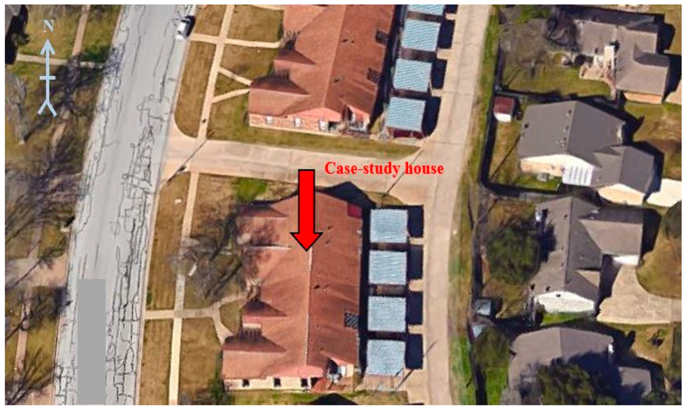
In this paper, a case study, single-family residence was used that is a one-story, fourplex townhouse, constructed in 1982, in central Texas. One occupant lived in the residence. On Fridays, it was observed that additional people often visited the residence during the evening. The case study residence has two bedrooms, and one and a half baths with a total conditioned floor area of 111 m2 (1199 ft2). The front of the residence faces west with covered parking on the east side of the residence. Two other townhouses are attached on the north and south sides, respectively. Figure 1 shows a bird’s eye view of the case study residence [20]. In February 2017, the existing thermostat was replaced with a new smart thermostat that provided measured interval data for occupancy, heating and cooling setpoints, inside air temperatures, inside relative humidity, and HVAC system on and off schedule in 5-min intervals. Although the 5-min intervals were selected using the manufacturer’s setting, the 5-min interval data were converted to hourly intervals for this paper. The details about the measurements at the site can be found in [19]. The indoor air temperature sensors and the occupancy sensors (i.e., Passive Infrared (PIR) sensor) were associated with the smart thermostat. However, additional data loggers for indoor air temperature and occupancy were installed by the researchers to compare the results from the thermostat sensors and the data loggers. The sensors and the data loggers were placed in each location by the researchers.
In this study, an improved building energy simulation model was developed using the measured data from a smart thermostat with remote and wireless inside temperature and occupancy sensors as well as measured energy use data from the smart meter (i.e., interval electricity use) that served the residence.
The tuning process used in this paper was manual. As a first step in the process for a building simulation model, initial parameters were determined for the case study residence, as shown in Table A1, using estimated and actual characteristics obtained from an onsite visit. Next, the 2000 or 2009 International Energy Conservation Code (IECC) performance path [21,22] and the information from the simulation program’s default library (i.e., nominal values) [23] were used for estimated information regarding the building energy simulation model inputs for the existing building.
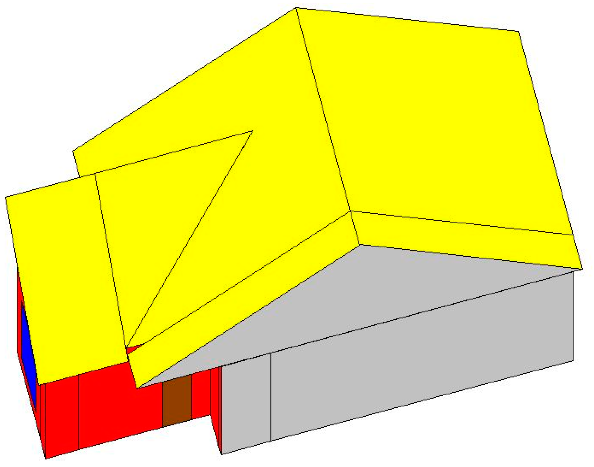
Figure 2 shows a rendering of the residential building simulation model of the case study residence using a visualization tool (i.e., DrawBDL [24]) that reads the input file of the DOE-2.1E program and draws the image. The DOE-2.1E simulation program was used for the analysis because it is a very reliable and well documented program that is accredited by Residential Energy Services Network (RESNET) for residential simulations of the code-compliant buildings using the Home Energy Rating System (HERS) index [25]. In the figure, the yellow surfaces are the roofs, the red surfaces are the exterior walls, the brown surfaces are the doors, the blue surfaces are the windows, and the gray surfaces are the interior walls that separate the residence from the adjacent residences.
Next, coincident weather data was collected from a nearby weather station that was approximately 9.2 km (5.8 miles) away from the case study residence. The weather data included 1-min interval data of dry-bulb temperature, wet-bulb temperature, dew-point temperature, wind speed, wind direction, global solar radiation, and direct normal solar radiation [26]. The measured weather data were converted into the appropriate hourly binary format for use by the building simulation model [23].
Figure 2.
The 3D view of the hourly building simulation model for the case study residence view of the case study residence [27].
Figure 2.
The 3D view of the hourly building simulation model for the case study residence view of the case study residence [27].

In addition, measured hourly occupancy data from the seven portable data loggers were collected for the model input. We measured the occupancy using the 1-min interval data from the occupancy data loggers of the seven zones. Then, we converted the 1-min interval data into the hourly interval data that represents the presence of an occupant over the period of one hour (i.e., diversity factor). The hourly occupancy diversity factors from the seven zones were then averaged. The average hourly occupancy diversity factor from the seven zones [19] was then used for the simulation to better represent the occupancy in the actual residence that had the single-zone HVAC system. The occupancy diversity factor was calculated using the ratio of the measured averaged occupancy from the seven zones to the maximum of occupancy (i.e., 1). Of special interest to this study, the measured hourly HVAC system operation status data and measured hourly heating and cooling setpoint data were also collected from the smart thermostat and used to improve the tuning process. In contrast to most of the previous studies (see the sixth column in Table 1), in this study the measured heating and cooling setpoints and the measured HVAC operation data were also used as model inputs. Then, after running the simulation model, the simulated hourly electricity use data and the simulated hourly indoor air temperature data were extracted from the simulation output file, and compared with the corresponding measured data during a one-week period.
As previously mentioned, measured hourly electricity use data was collected from the smart meter at the case study residence. In addition, measured hourly indoor air temperatures from the seven portable wireless sensors were collected. An additional indoor air temperature sensor, at the location of the actual thermostat, was installed to identify the indoor air temperature profile near the thermostat. The other seven indoor air temperature profiles were averaged, and compared with the simulated, single indoor air temperature profile output since the simulation model had a single-zone residential HVAC system that assumed a well-mixed, single indoor air temperature. A single-zone system was chosen for the simulation analysis because it was more representative of the system used in the actual case study residence that had one thermostat in the hallway. Using measured data from the seven indoor air temperature sensors at different locations, inside air temperature versus ambient air temperature profiles were also generated [19]. It was found that the indoor air temperature profiles were significantly different between the seven locations as well as different from the profiles of the heating and cooling setpoints.
Finally, whole-building electricity use data and indoor air temperature data were used for the model outputs in terms of the tuning process. In summary, compared to the previous studies, the measured hourly whole-building electricity use and the measured hourly indoor air temperature data, as well as the measured hourly heating and cooling setpoints and the measured hourly HVAC system operation status data from a smart thermostat, were used for the tuning process in this study.
Multiple simulation runs were conducted where the input parameters were adjusted in order for the simulated whole-building electricity use to better match the measured whole-building electricity use. Mean Bias Error (MBE) (kWh), Normalized Mean Bias Error (NMBE) (%), and Coefficient of Variation of the Root Mean Square Error (CV-RMSE) (%) were used as the goodness-of-fit indicators [28,29]. To match the simulated indoor air temperatures (IATs) with measured indoor air temperatures, the MBE (°C), NMBE (%), and CV-RMSE (%) were used. In this process, several different approaches were used to adjust the input parameters, including: fixing the simulation input parameters to values obtained from an onsite visit; information from the 2000/2009 IECC; simulation libraries; and measured data (i.e., estimated/fixed model inputs). Adjusting the simulation was then accomplished by adjusting the other estimated simulation inputs to obtain a better prediction of the whole-building electricity use and the indoor air temperatures (i.e., the tuning process). Again, it is worth noting that measured hourly heating and cooling setpoints and measured hourly HVAC system operation status data from a smart thermostat were used as fixed model inputs, whereas the hourly measured whole-building electricity use and hourly measured indoor air temperature data were used for the tuning process.
For the MBE, Equation (1) was used since the absolute scale of the hourly electricity use data and hourly indoor air temperature were significantly different. In the analysis, MBE was calculated to see how the measured values were different from the simulated values. Positive values represent the under prediction of the simulation results, and smaller values indicate less differences [29].
where is the measured data, is the simulated data by the building simulation model, n is the number of data points, and p is the number of parameters (i.e., p is 1 in this paper for the tuning process [28]).
The NMBE using Equation (2) was also used to indicate normalized, biased errors by dividing MBE by the average value of the measured data [29]. In addition, CV-RMSE using Equation (3) was used to represent how well the simulation model predicts the measured data. Smaller NMBE and CV-RMSE values indicate less biased errors and better models, respectively. MBE, NMBE, and CV-RMSE were simultaneously used to better compare the simulated results with the measured data, observing the degree of the simulation model errors and the confidence of the model. These three indicators are recommended by ASHRAE Guideline 14 [28].
3. Results
Table 2 shows a summary of the individual parameter changes during the entire process and the corresponding statistical indices of both the indoor air temperatures and the whole-building electricity use. From Run #1 to Run #2, the process was conducted with the fixed model inputs using estimated information and measured data. From Run #3 to Run #5, the process was conducted with estimations used in Run #1 and Run #2 replaced by measured inputs. From Run #6 to Run #10, the process further tuned the model by adjusting the estimated model inputs based on the comparison of simulated and measured outputs.
Run #1 shows the simulation results of the nominal base-case model. The nominal base-case model was created using an estimated constant heating setpoint of 22 °C (72 °F) and constant cooling setpoint of 26 °C (79 °F) for all hours for the period from 20 February 2017 to 26 February 2017. These setpoints were obtained from the occupant. Occupancy, lighting, and equipment schedules were also estimated for the model inputs based on communications with the occupant.
For Run #2, to better match the measured indoor air temperatures and whole-building electricity use, the lighting and equipment schedules were fixed based on the estimation from the measured occupancy data of the seven occupancy sensors. In addition, occupancy schedules in the simulation were directly fixed using the measured occupancy data. This parameter change slightly worsened the statistical indices of the indoor air temperatures, but significantly improved the indices of the whole-building electricity use, when they were compared to Run #1. This improvement was reasonable because the lighting and equipment schedules directly impact the whole-building electricity use for many of the hours of the measurement period.
For Run #3, the heating and cooling setpoints of the building simulation model were fixed using the measured average indoor air temperatures. At this step, it should be noted that the measured average indoor air temperature from all the seven zones was used to fix the thermostat schedule of the simulation model to better match the simulated indoor air temperatures with the measured indoor air temperatures. This resulted in a significantly improved goodness-of-fit for the indoor air temperatures (i.e., MBE of 0.04 °C, NMBE of 0.11%, and CV-RMSE of 0.17%). However, the simulation still did not exactly match the measured whole-building electricity use because the simulated HVAC system was running more often than the measured HVAC system operation status. As a result, in Run #3, the building simulation model showed MBE of −0.56 kWh, NMBE of −92.07% and CV-RMSE of 135.44% for the whole-building electricity use, which resulted in increasing the absolute value of MBE of 0.15 kWh with NMBE of 22.15% and CV-RMSE of 9.75%, when they were compared to Run #2.
For Run #4, the heating and cooling setpoints were again fixed using the measured setpoint data from the smart thermostat. Run #4 and subsequent runs (#5 through #10) did not include the fixed heating and cooling setpoints using the measured average indoor air temperatures, shown in Run #3. The results of Run #4 showed that the setpoint changes using the measured setpoint data made a large difference between the measured indoor air temperatures and the simulated indoor air temperatures because the base-case building model’s characteristics of the residence, such as the thermal mass, did not exactly match with the actual building’s characteristics. However, this setpoint change in Run #4 improved the goodness-of-fit of the simulated whole-building electricity use because it helped to correct the runtime of the heating and cooling system when indoor air temperatures were below the heating setpoint or above the cooling setpoint. As a result, Run #4 showed improved statistical indices with NMBE of 0.11% and CV-RMSE of 1.81% for the whole-building electricity use, when they were compared to Run #2. MBE for the whole-building electricity use was slightly increased to 0.01 kWh.
For Run #5, the heating and cooling system schedules were fixed using the measured HVAC system operation status data (i.e., system on and off), which was available from the smart thermostat. Unfortunately, the system schedule change significantly worsened the differences between the measured indoor air temperatures and the simulated indoor air temperatures (i.e., MBE of 2.43 °C, NMBE of 5.93%, and CV-RMSE of 6.30% compared to Run #4) because the base-case simulation model did not have accurate building characteristics for the indoor environment. However, the system schedule change significantly improved the goodness-of-fit of the whole-building electricity use because the schedule corrected the runtime of the simulated heating and cooling system to match the actual system runtime. As a result, Run #5 showed significant improvements for the absolute value of MBE of 0.42 kWh with NMBE of 68.02% and CV-RMSE of 28.77% for the whole-building electricity use, when they were compared to Run #4.
Run #6 shows the results from the use of an effective U-value [30] used for the case study house’s slab-on-grade floor. In this run, the effective U-value was adjusted from 0.442 W/m2-K (0.078 Btu/hr-ft2-°F), which was calculated using the underground surface heat transfer calculation method [31], to 0.006 W/m2-K (0.001 Btu/hr-ft2-°F), which better represented the conductive heat transfer of the actual building. The adjustment improved the goodness-of-fit of both the statistical indices of the indoor air temperatures and the whole-building electricity use compared to Run #5 (i.e., the absolute value of MBE of 1.36 °C with NMBE of 3.31% and CV-RMSE of 2.63% for the indoor air temperatures, as well as NMBE of 0.49% and CV-RMSE of 11.26% for the whole-building electricity use). MBE for the whole-building electricity use was slightly increased to 0.02 kWh.
Run #7 shows the results of adjusting the effective window frame conductance from 17.23 W/m2-K (3.04 Btu/hr-ft2-°F) to 5.67 W/m2-K (1.00 Btu/hr-ft2-°F). In this run, the adjustment slightly improved the goodness-of-fit of the indoor air temperatures. However, it did not improve the goodness-of-fit of the whole-building electricity use. This same trend was also seen when the effective wall R-value was adjusted.
Run #8 shows the improved results from modifying the DOE-2.1E weighting factors from 0 to 635 kg/m2 (130 lb/ft2), where the weighting factors of “0” are used for DOE-2′s custom weighting factors. The pre-calculated weighting factor of 635 kg/m2 (130 lb/ft2) was used to estimate the characteristics of the thermal mass in the residence. Since the material properties of the actual floor, walls, and ceiling were not specifically known for the simulation model, the pre-calculated weighting factors gave a more reasonable fit for simulated the indoor air temperatures. However, it worsened the goodness-of-fit of the simulated whole-building electricity use versus the measured whole-building electricity use.
Run #9 shows improved results by changing the infiltration rate from 3 ACH50 to 0.03 ACH50 when the heating or the cooling system was on. This adjustment estimated a reduced infiltration rate when the HVAC system was turned on because the system slightly pressurized the house. The change improved the goodness-of-fit of the indoor air temperatures. In addition, the change improved CV-RMSE of the whole-building electricity use. However, the change worsened NMBE of the whole-building electricity use.
Run #10 was the final tuning step. This step modified the lighting, equipment, and Domestic Hot Water (DHW) system schedules based on the measured occupancy schedules, the measured HVAC system on/off operation status, and information from the analysis of the whole-building electricity use data from the previous study [32] to identify end-use energy patterns. The modification significantly increased the goodness-of-fit of both the indoor air temperatures and the whole-building electricity use, when they were compared to Run #9 (i.e., the absolute values for MBE of 0.24 °C, NMBE of 0.60%, and CV-RMSE of 0.39% for the indoor air temperatures, as well as MBE of 0.12 kWh, NMBE of 15.61% and CV-RMSE of 58.87% for the whole-building electricity use). It should be noted that the profiles between the measured and simulated indoor air temperatures still showed differences even though the statistical indices showed an improved goodness-of-fit. The reason for this seems to be that the estimated information for the model inputs still contained some uncertainty.
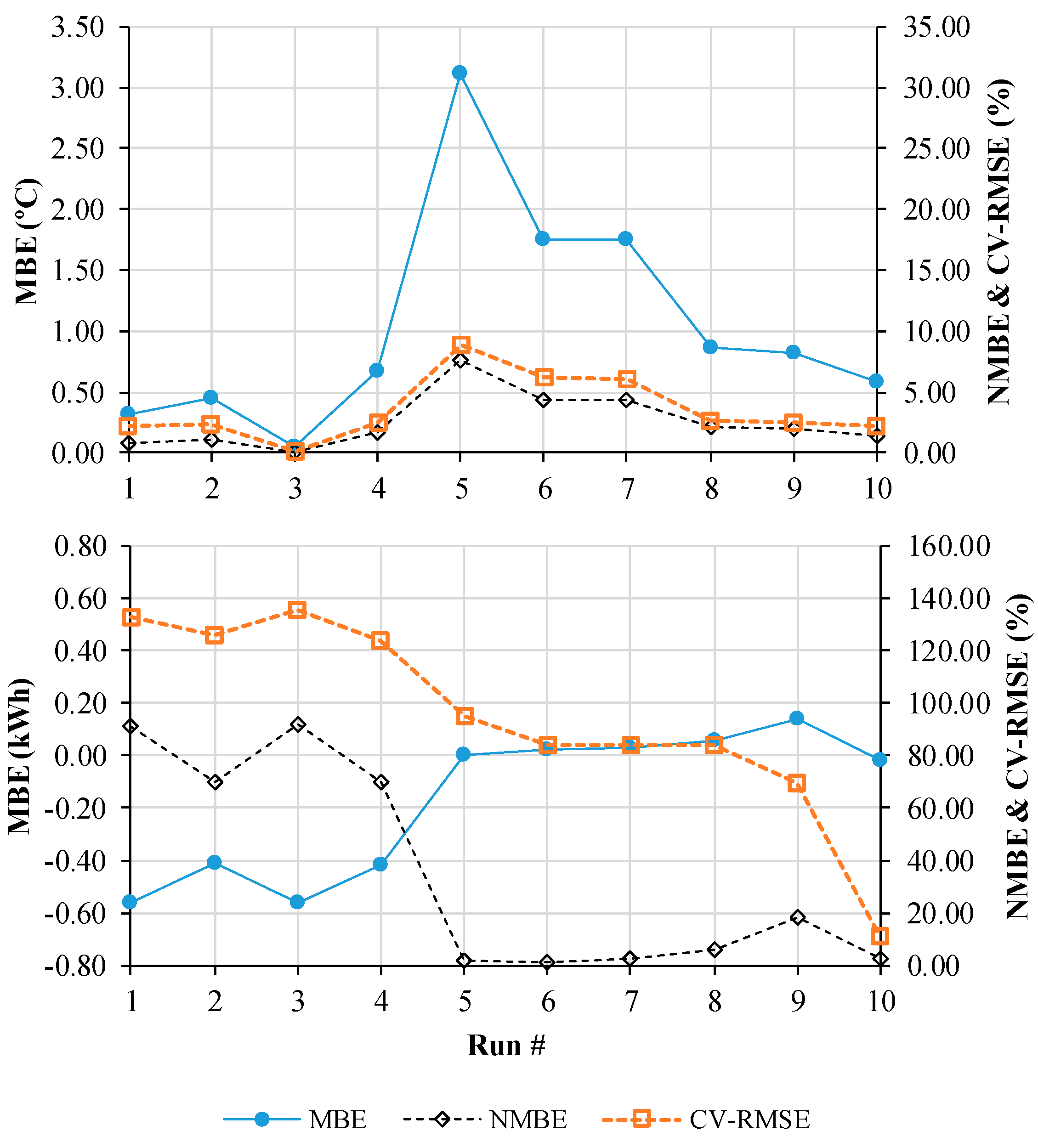
Figure 3 shows the results from the statistical indices of Table 2. For the indoor air temperatures, the significant improvements occurred from Run #5 to Run #6 and from Run #7 to Run #8 when the effective U-value of the floor was adjusted and the weighting factors were adjusted, respectively. The effective U-value was related to the conductive heat transfer, and the weighting factor was related to the thermal mass effect (i.e., thermal radiation). For the whole-building electricity use, the significant improvements occurred from Run #4 to Run #5 and from Run #9 to Run #10 when the heating and cooling system operation status was fixed to match the measured HVAC operation status, and the lighting, equipment, and DHW system schedules were adjusted, respectively. These parameters significantly affected the building energy consumption.
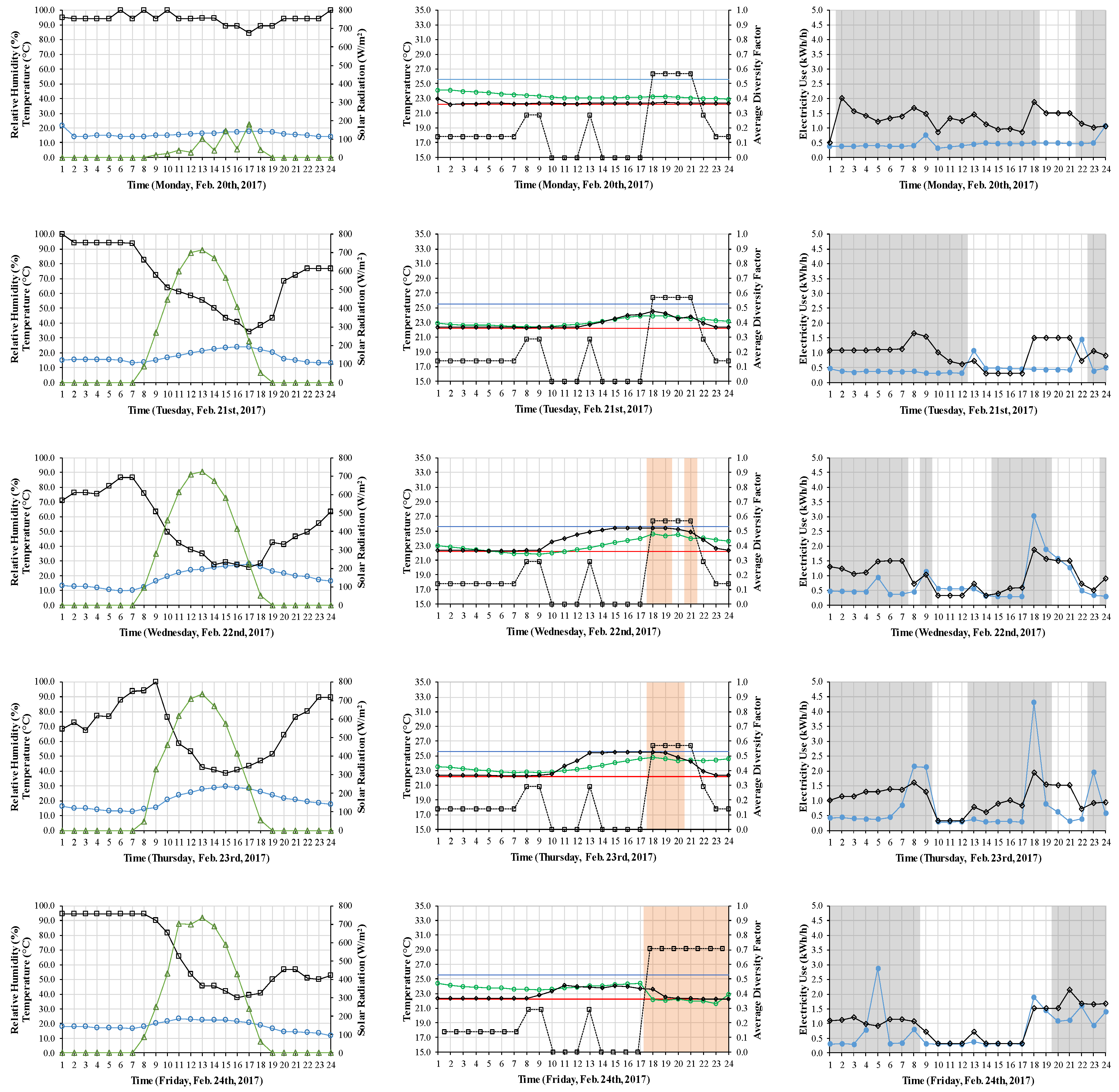
Figure 4 shows the measured weather data (upper plot), the simulated indoor environmental conditions and the measured HVAC system operation (middle plot), and the simulated/measured whole-building electricity use and the simulated HVAC system operation status (lower plot) for Run #1 (i.e., the initial stage). The measured HVAC system operation (i.e., the vertical tan-colored bars in the middle plot) was not used for the model input for Run #1. However, it is displayed in this figure so the reader can compare the measured HVAC system operation with the simulated HVAC system operation (i.e., the vertical grey bars in the lower plot). The vertical grey bars for the simulated HVAC system operation indicate when the simulated heating (i.e., the red line with a square marker) or cooling (i.e., the blue line with a triangle marker) energy use occurred.
The constant heating/cooling setpoints, and the assumed occupancy, lighting, and equipment schedules, are also shown in the middle plot of Figure 4. They were estimated for Run #1. This juxtaposed, superimposed, time-series figure [33] effectively shows the exact differences of the detailed trends between the simulated and measured data. In the middle plot, the difference between the measured indoor air temperatures (the green line) and the simulated indoor air temperatures (the black line) can be clearly seen.
For example, in Figure 4, it can be seen that the simulated indoor air temperatures changed more quickly than the measured indoor air temperatures, which implies that the simulated building lost or gained heat more quickly through the building envelope versus the observations from the case study building. For example, on Wednesday, February 22, 2017, which was a clear spring day, the simulated indoor air temperatures picked up quickly in the morning as soon as the solar radiation picked up. However, the average measured indoor air temperatures from the seven sensors and the measured temperature at the thermostat increased at a slower rate. In addition, in the afternoon on that same day, the simulated indoor air temperatures dropped rapidly, while the average measured indoor air temperatures slowly decreased.
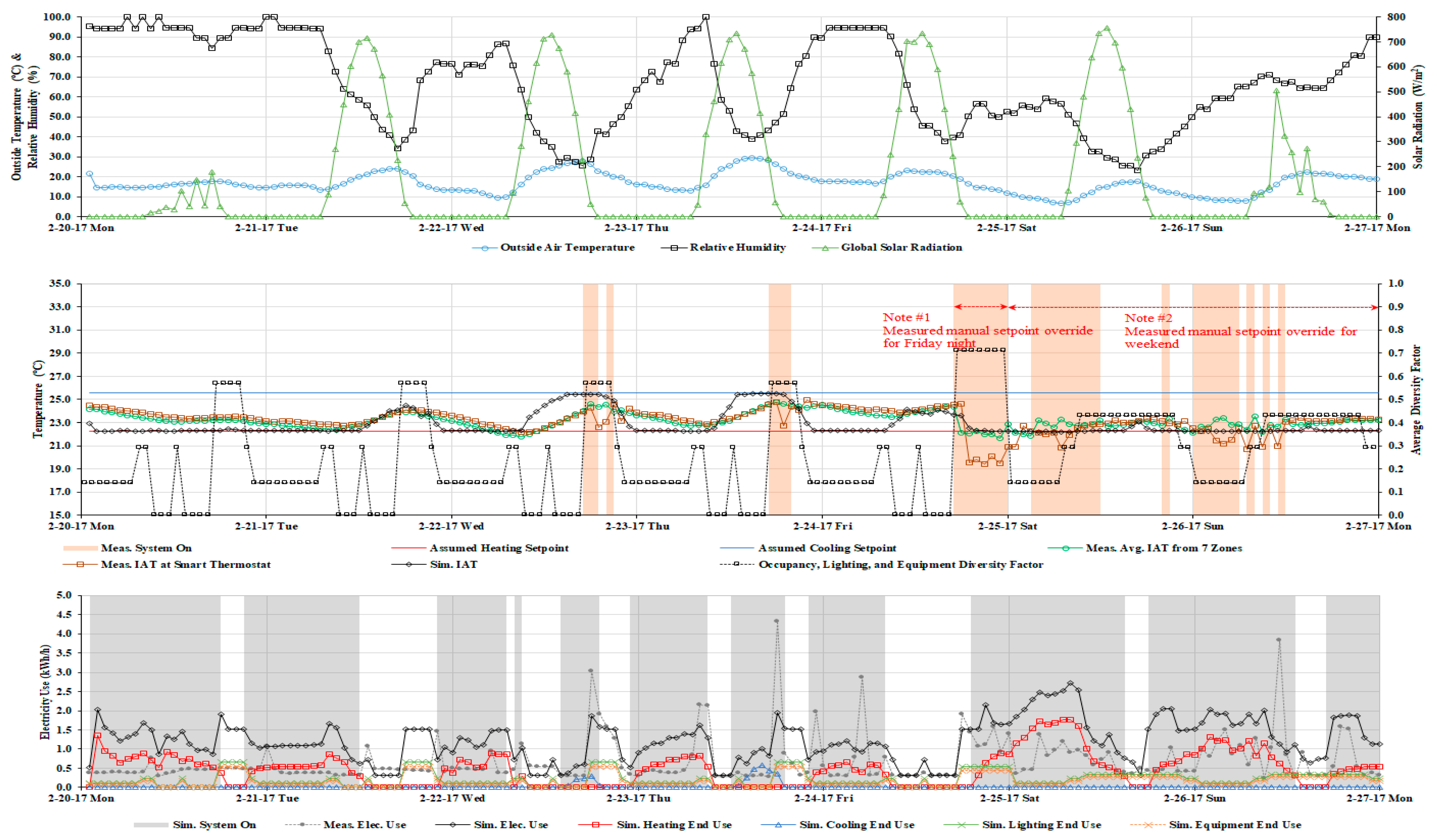
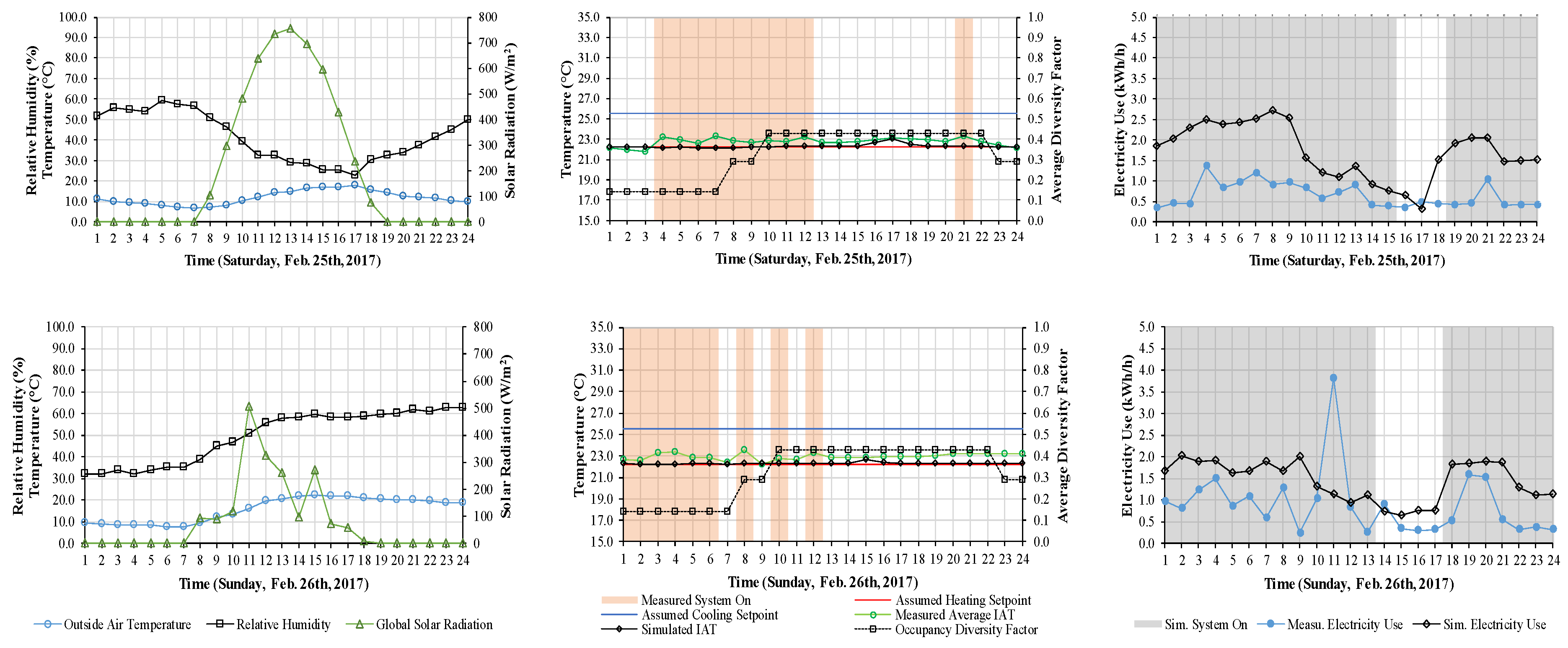
Figure 5 shows the hourly differences between the simulated and measured data at Run #10 (i.e., the final stage). In the middle plot, improvements in the differences between the measured indoor air temperature (the green line) and the simulated indoor air temperature (the black line) can be seen. The middle plot also shows the dynamic measured heating and cooling setpoints of the smart thermostat that uses the occupancy schedules and the indoor air temperature (the blue and red lines). Note #1 and Note #2 show the times when the occupant overrode the manual setpoints. In addition, the middle plot shows that the times when the HVAC system was turned on using the measured system status data from the smart thermostat. For example, on Saturday, 25 February 2017 at 8:00 p.m., the heating system was turned on, which resulted in the simulated heating energy use of 0.5 kWh as shown in the lower plot (the red line with the square marker). At Run #10, the simulated HVAC system operation shown in the lower plot was forced to match the measured operation shown in the middle plot. In addition, the measured occupancy diversity factors in the middle plot show that most of the diversity factors were above 0, which indicates the occupant stayed at home during this time period. For example, on Thursday, 23 February 2017 at 12:00 p.m., the occupant came back home for lunch and moved around the six zones (i.e., 0.86). It is also shown that the smart thermostat automatically changed the heating and cooling setpoints to the higher heating setpoint and the lower cooling setpoint by detecting the occupant. In the lower plot, the results for Run #10 show the simulated whole-building electricity use was well matched with the measured whole-building electricity use. In addition, the simulated end-use electricity use was displayed to observe estimated energy behaviors from the simulation model.
In general, this level of detailed plots and analysis for the tuning process (i.e., Figure 4 and Figure 5) is a very useful tool for simulators to better understand the accuracy and reliability of their building simulation models. In this study, it was found that these juxtaposed, superimposed time series plots allowed for the exact observation of the simulated/measured indoor environment and energy behaviors, as well as system operation status, with special attention paid to the temporal characteristics during the tuning process.
4. Discussion
The tuning process developed in this study provided several new improvements over the previous studies. First, the improved building energy simulation model better predicted the measured average hourly indoor air temperature profile during the tuning period (see Figure 5). Although several studies [10,11,12,13,14,15,16,17] reported that they studied how the indoor air temperatures can be used in the calibration approaches, they did not analyze a dynamic profile of the indoor air temperatures to improve the outputs of simulation models during the calibration steps. In addition, the previous studies did use the indoor air temperature profile that were measured at one or two locations. Therefore, by using simultaneous measurements of whole-building electricity use and an indoor air temperature profile, averaged from all the zones, the results from the tuning process of the residential building energy simulation model used in this study showed an improvement in the reliability of the model for energy efficiency and comfort analyses.
Second, the sequence that was developed for tuning the simulation model utilized three multi-stage steps: (1) it used estimated information for fixed model inputs, (2) it used measured data for fixed model inputs (e.g., solar radiation, outside humidity, outside air temperature, inside air temperature, etc.), and (3) it used measured data for model tuning. In this study, the measured data for fixed model inputs (i.e., measured occupancy data, measured heating and cooling setpoints, and measured HVAC system’s on and off schedule) were used to help create an improved building energy simulation model. Particularly, it was found that the HVAC system’s on and off schedule from the smart thermostat was a significant parameter affecting the results of the tuning process. The multi-stage approach using the measured indoor environmental data and the measured HVAC operation data improved the tuning process when using a simulation model for both the comfort analysis and the energy use analysis. However, for a future study, it was found that there is a need to better predict energy-related and non-energy-related occupancy profiles using measured data. Although the internal heat gains from the occupant(s) are estimated, the use of the system (e.g., HVAC system and other appliances such as lighting and dryers) on and off schedules can significantly change the accuracy of the simulation of the whole-building energy use.
Third, a detailed one-week period was used to demonstrate the tuning process using juxtaposed, superimposed, time series plots. This process compared measured and simulated hourly-interval indoor air temperatures and whole-building energy use. The goal of this paper was to observe how close a simulation program could predict not only indoor air temperature but also whole-building energy use. Thus, a one-week period of detailed measured data was used because the one week that was chosen had both periods of heating and cooling as well as the periods when HVAC system was on and off, including the periods when the inside temperatures reached heating and cooling setpoints.
The model developed in this study was used to demonstrate how to make a simulation model more closely match the measured energy use and indoor air temperatures in the case study residence that has data from a smart thermostat (i.e., HVAC system on and off data and coincident heating/cooling setpoints data) and smart sensors (i.e., inside temperature data and occupancy detection data in each room). The results of this study showed that the simulation results can be closely matched with the measured data. In addition, tracking each tuning steps allows for a detailed inspection of each step of the process that better identifies why the simulation result is different from the measured data, and how each parameter contributed to the tuning process. In contrast to most of the previous studies, this study found that the simulated hourly HVAC system on and off status was needed to better match the actual hourly HVAC system on and off status in order to accomplish the most accurate tuning process for the whole-energy use simulation. This is an important feature for a well-tuned simulation that is used to simulate a residence with an occupancy- and temperature-based thermostat control. In future work, a method to predict the HVAC system on and off status against outside air temperature needs to be developed for more accurate residential simulation models. In addition, the smart thermostat used in this study had 5 min intervals to indicate the HVAC system on and off. However, it did not have runtime data. Thus, future smart thermostats will need to provide the runtime information to provide more accurate data for the tuning/calibration approach about how many minutes the system is on during the interval period.
The tuning approach developed in this paper is also very important for the smart greenhouse building that uses the HVAC system to maintain the optimal indoor air temperature range for growing vegetables and fruits [34,35]. In addition to residential buildings, the simulation model that reflects the dynamics of indoor air temperature and whole-building energy use can be effectively used to find the scenarios to increase the products as well as to save energy use in smart greenhouse buildings.
The limitations of this study include the uncertainty of the estimated information that was used (i.e., building parameters) such as wall R-value and window U-factor for model inputs, as well as the impact of the adjusted lighting and equipment schedules in the simulation. This study found that such information for the building input parameters is important for a building energy simulation model. However, the detailed information is not always available, especially for older, existing residential buildings. Thus, the availability of data from the smart thermostat is significant to create better residential models [36,37,38].
5. Conclusions and Future Work
This paper presents the results from the analysis of an improved tuning procedure for a residential building that uses smart thermostat and smart meter data. The improved procedure using a side-by-side comparison based on the individual parameter changes was developed to better match both the whole-building energy use and indoor air temperature. In this paper, three approaches were identified for the tuning process: (1) estimated information for fixed model inputs, (2) measured data for fixed model inputs, and (3) measured data for model tuning. The use of estimated information for model inputs is a widely-used approach to create an initial simulation model using information from an onsite visit, equipment installed onsite, building energy standards, and simulation program default libraries. However, in this study, measured data from various sensors at the case study site was used to help tune model inputs to onsite conditions. Particularly, HVAC system on/off operation status data and heating and cooling setpoint data from a smart thermostat installed at the case study site were used to improve the residential building energy model that matches the measured data.
Using both the measured indoor air temperature and measured whole-building energy use data, a residential building energy simulation model was tuned at the hourly level. We found that the most significant parameters for predicting the indoor air temperature and whole-building energy use were the effective U-value of a slab-on-grade floor and the heating and cooling system operation status, respectively. To effectively tune a simulation model, it is recommended that the most influential parameters be identified first in the tuning process that this paper developed.
This paper used statistics (see Figure 3) and graphical displays (see Figure 4, Figure 5, Figure A1 and Figure A2) to improve the hourly tuning process. These graphical displays provided detailed plots for the tuning process that helped to better understand how the building energy simulation model changed to better match the hour-by-hour indoor environment and energy use during the tuning process. These results also imply that high frequency (i.e., small time intervals) measurements help improve the accuracy of the tuning process. Tracking each of tuning steps through statistics and graphical displays can easily detect the differences in the simulated vs. measured building system data by identifying why the simulation result is different from the measured data.
For a future study, additional tools for improved matching during the calibration process need to be developed, including new statistical indices [39] for the calibration of indoor environmental data and new, more effective graphical calibration displays as shown in Figure 4, Figure 5, Figure A1 and Figure A2. Even though the suggested approaches were developed using a manual tuning process, these approaches could be applied to an automated calibration process. Based on the results of this study, the use of a regression model is proposed that uses outdoor/indoor air temperatures, whole-building energy use, and system on/off status for the tuning process. In addition, there is a need to better predict HVAC system on and off status for the annual-period tuning process.
As more data from smart technologies and/or Internet of Things (IoT) in residential and other buildings become available, the approaches described in this study will be useful for building energy modelers.
Author Contributions
Conceptualization, S.O.; methodology, S.O., J.-C.B. and J.S.H.; software, S.O.; validation, S.O.; formal analysis, S.O.; investigation, S.O.; resources, S.O.; data curation, S.O.; writing—original draft preparation, S.O.; writing—review and editing, J.-C.B. and J.S.H.; visualization, S.O.; supervision, J.-C.B. and J.S.H. All authors have read and agreed to the published version of the manuscript.
Funding
This research received no external funding.
Institutional Review Board Statement
Not applicable.
Informed Consent Statement
Not applicable.
Data Availability Statement
Not applicable.
Acknowledgments
This work was supported by the Korea Institute of Energy Technology Evaluation and Planning (KETEP) and the Ministry of Trade, Industry & Energy (MOTIE) of the Republic of Korea (No. 20212020800050). Work on this project was partially supported by the ASHRAE Graduate Student Grant-In-Aid for the 2016–2017 academic year, as well as the Texas Emissions Reduction Program (TERP).
Conflicts of Interest
The authors declare no conflict of interest.
Appendix A

Table A1.
Parameters used for the initial simulation in the case study residence.
| Construction | |
|---|---|
| Residence type | Townhouse, attached house |
| Constructed year | 1982 |
| Orientation | West |
| Gross area | 111 m2 |
| Number of floors | 1 |
| Height | 2.7 m |
| Construction | Wood |
| Floor | Slab on grade |
| Wall color | Dark |
| Wall area | 133 m2 |
| Wall R-value | 2.16 m2-K/W (12.24 hr-ft2-°F/Btu) |
| Stud spacing | 38.1 mm × 88.9 mm (2 in × 4 in nominal) |
| Window type | Single pane |
| Window area | 10 m2 |
| Window frame type | Aluminum or steel |
| Window U-factor | 0.11 W/m2-K (0.65 Btu/hr-ft2-°F) |
| Window SHGC | 0.30 |
| Roof configuration | Unconditioned, vented attic |
| Roof color | Medium |
| Roof R-value | 4.90 m2-K/W (27.8 hr-ft2-°F/Btu) |
| Roof slope | 45° |
| Space conditions | |
| Number of occupants | 1 |
| Setpoint | Heating 23.3 °C (74.0 °F)/Cooling 23.9 °C (75.0 °F) |
| Heating and Cooling system | |
| Fuel | Electricity |
| System Type | Heat pump (Air to Air) |
| Capacity | 7 kW |
| Heating Efficiency | HSPF 6.8 |
| Cooling Efficiency | SEER 10 |
| System Location | Attic |
| Condenser Location | Outside |
| Manufacturer/year | Goodman CPKJ30-10/approx. 2006 |
| DHW system | |
| Fuel | Electricity |
| Capacity | 0.15 m3 |
| Efficiency | 1.0 |
| Location | Conditioned zone |
| Manufacturer/year | Whirlpool model # EE2H4DRX9R5V/Unknown |
| Appliances | |
| Internal equipment | 1-Refrigerator, 1-clothes washer, 1-clothes dryer, 1-dish washer, 1-range and oven, 2-television, and 1-laptop |
| Lighting | Interior lighting: 20-overhead light bulbs and 1-standing lamp Exterior lighting: 1-light bulb |
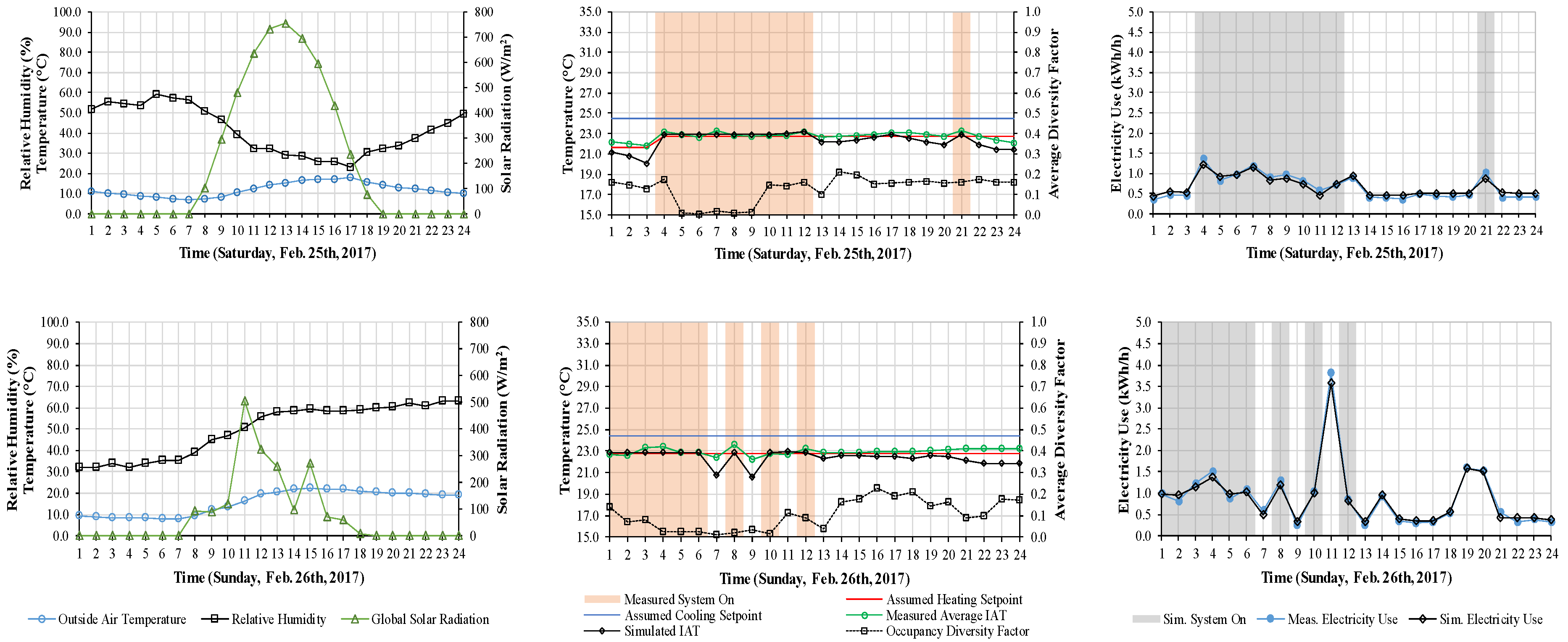
Figure A1.
Run #1 base-case simulation model results showing IATs, coincident weather data, and electricity use from Monday to Sunday (from 20 February 2017 to 26 February 2017).
Figure A1.
Run #1 base-case simulation model results showing IATs, coincident weather data, and electricity use from Monday to Sunday (from 20 February 2017 to 26 February 2017).


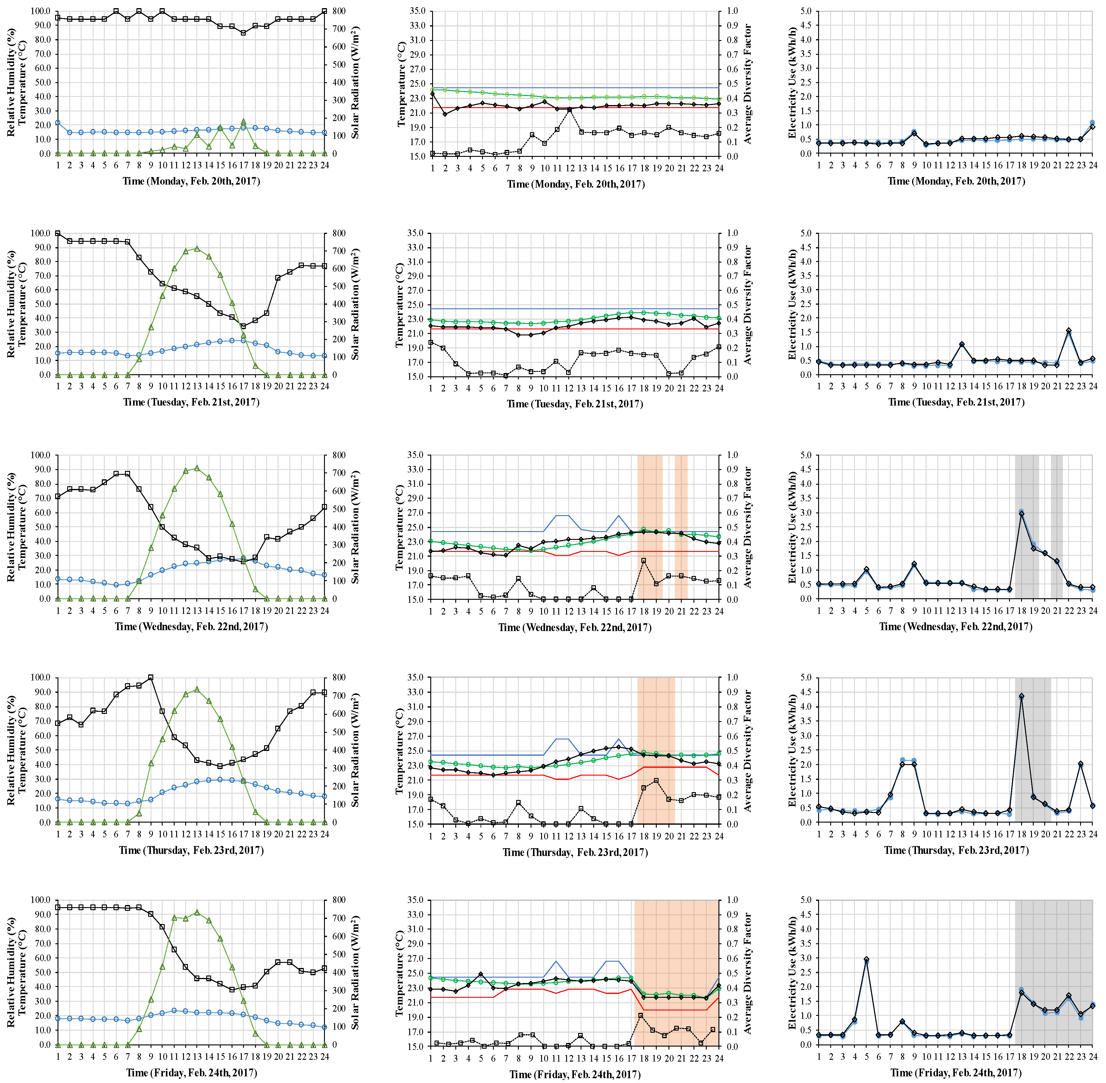
Figure A2.
Run #10 simulation model results showing IATs, coincident weather data, and electricity use from Monday to Sunday (from 20 February 2017 to 26 February 2017).
Figure A2.
Run #10 simulation model results showing IATs, coincident weather data, and electricity use from Monday to Sunday (from 20 February 2017 to 26 February 2017).


References
- ASHRAE. Chapter 19: Energy Estimating and Modeling Methods. In ASHRAE Handbook–Fundamentals; ASHRAE: Atlanta, GA, USA, 2017. [Google Scholar]
- Coakley, D.; Raftery, P.; Keane, M. A Review of Methods to Match Building Energy Simulation Models to Measured Data. Renew. Sustain. Energy Rev. 2014, 37, 123–141. [Google Scholar] [CrossRef] [Green Version]
- Reddy, T.A. Literature Review on Calibration of Building Energy Simulation Programs: Uses, Problems, Procedures, Uncertainty, and Tools. ASHRAE Trans. 2006, 112, 226–240. [Google Scholar]
- Fabrizio, E.; Monetti, V. Methodologies and advancements in the calibration of building energy models. Energies 2015, 8, 2548–2574. [Google Scholar] [CrossRef] [Green Version]
- Mustafaraj, G.; Marini, D.; Costa, A.; Keane, M. Model calibration for building energy efficiency simulation. Appl. Energy 2014, 130, 72–85. [Google Scholar] [CrossRef]
- Robertson, J.; Polly, B.; Collis, J. Evaluation of Automated Model Calibration Techniques for Residential Building Energy Simulation; National Renewable Energy Lab.(NREL): Golden, CO, USA, 2013.
- Manke, J.M.; Hittle, D.C.; Hancock, C.E. Calibrating Building Energy Analysis Models Using Short Term Test Data. In Proceedings of the International Solar Energy Conference, San Antonio, TX, USA, 31 March–3 April 1996; ASME: San Antonio, TX, USA, 1996. [Google Scholar]
- Tian, W.; Heo, Y.; de Wilde, P.; Li, Z.; Yan, D.; Park, C.S.; Feng, X.; Augenbroe, G. A Review of Uncertainty Analysis in Building Energy Assessment. Renew. Sustain. Energy Rev. 2018, 93, 285–301. [Google Scholar] [CrossRef] [Green Version]
- US Department of Energy Emerging Technologies Research and Development. DRAFT Research and Development Opportunities for Building Energy Modeling; US DOE: Washington, DC, USA, 2019.
- Hsieh, E.S. Calibrated Computer Models of Commercial Buildings and Their Role in Building Design and Operation; Princeton University: Princeton, NJ, USA, 1988. [Google Scholar]
- Bou-Saada, T.E. An Improved Procedure for Developing a Calibrated Hourly Simulation Model of an Electrically Heated and Cooled Commercial Building; Texas A&M University: College Station, TX, USA, 1994. [Google Scholar]
- Coakley, D.; Raftery, P.; Molloy, P. Calibration of Whole Building Energy Simulation Models: Detailed Case Study of a Naturally Ventilated Building Using Hourly Measured Data. In First Building Simulation and Optimization Conference; IBPSA-England: Loughborough, UK, 2012; pp. 57–64. [Google Scholar]
- Lam, K.P.; Zhao, J.; Ydstie, E.B.; Wirick, J.; Qi, M.; Park, J. An Energyplus Whole Building Energy Model Calibration Method for Office Buildings Using Occupant Behavior Data Mining and Empirical Data. In Proceedings of the Building Simulation Conference, Atlanta, GA, USA, 10–12 September 2014; ASHRAE/IBPSA-USA: Atlanta, GA, USA, 2014; pp. 160–167. [Google Scholar]
- Royapoor, M.; Roskilly, T. Building Model Calibration Using Energy and Environmental Data. Energy Build. 2015, 94, 109–120. [Google Scholar] [CrossRef] [Green Version]
- Paliouras, P.; Matzaflaras, N.; Peuhkuri, R.H.; Kolarik, J. Using Measured Indoor Environment Parameters for Calibration of Building Simulation Model-A Passive House Case Study. Energy Procedia 2015, 78, 1227–1232. [Google Scholar] [CrossRef] [Green Version]
- Goldwasser, D.; Ball, B.; Farthing, A.; Frank, S.; Im, P. Advances in Calibration of Building Energy Models to Time Series Data. In Proceedings of the ASHRAE Building Performance Analysis Conference, Chicago, IL, USA, 26–28 September 2018; ASHRAE: Chicago, IL, USA, 2018. [Google Scholar]
- Kim, H.; Oldham, E. Energy Performance of an Occupancy-Based Climate Control (OBCC) Technology in Guest Rooms. ASHRAE Trans. 2019, 125, 703–717. [Google Scholar]
- Norford, L.K.; Socolow, R.H.; Hsieh, E.S.; Spadaro, G.V. Two-to-One Discrepancy between Measured and Predicted Performance of a “low-Energy” Office Building: Insights from a Reconciliation Based on the DOE-2 Model. Energy Build. 1994, 21, 121–131. [Google Scholar] [CrossRef]
- Oh, S.; Haberl, J.S.; Baltazar, J.C. Analysis of Zone-by-Zone Indoor Environmental Conditions and Electricity Savings from the Use of a Smart Thermostat: A Residential Case Study. Sci. Technol. Built Environ. 2020, 26, 285–303. [Google Scholar] [CrossRef]
- Google Google Map. Available online: https://www.google.com/maps (accessed on 15 May 2017).
- International Code Council. 2000 International Energy Conservation Code; ICC, Inc: Washington, DC, USA, 2000. [Google Scholar]
- International Code Council. 2009 International Energy Conservation Code; ICC, Inc: Washington, DC, USA, 2009. [Google Scholar]
- Winkelmann, F.C.; Birdsall, B.E.; Buhl, W.F.; Ellington, K.L.; Erdem, A.E.; Hirsch, J.J.; Gates, S. DOE-2 Supplement Version 2.1E (No. LBL-34947); Lawrence Berkeley Lab.: Berkeley, CA, USA; Hirsch (James J.) and Associates: Camarillo, CA, USA, 1993. [Google Scholar]
- Huang, J. Building Energy Simulation User News; Lawrence Berkeley National Laboratory: Berkeley, CA, USA, 2002; Volume 23, p. 13. [Google Scholar]
- RESNET. Accredited HERS Software Tools. Available online: https://www.resnet.us/providers/accredited-providers/hers-software-tools/ (accessed on 15 January 2022).
- Baltazar, J.C.; Haberl, J.S.; Yazdani, B.; Patrick, P.; Ellis, S.; Zilbershtein, G.; Claridge, D.E. Energy Efficiency/Renewable Energy Impact in the Texas Emissions Reduction Plan (TERP): Volume I-Technical Report; Energy Systems Laboratory: College Station, TX, USA, 2019. [Google Scholar]
- Oh, S. Quantifying the Electricity Savings from the Use of Home Automation Devices in a Residence; Texas A&M University: College Station, TX, USA, 2017. [Google Scholar]
- ASHRAE. ASHRAE Guideline 14-2014; ASHRAE: Atlanta, GA, USA, 2014. [Google Scholar]
- Ruiz, G.R.; Bandera, C.F. Validation of Calibrated Energy Models: Common Errors. Energies 2017, 10, 1587. [Google Scholar] [CrossRef] [Green Version]
- Andolsun, S.; Culp, C.H.; Haberl, J.; Witte, M.J. EnergyPlus vs. DOE-2.1e: The Effect of Ground-Coupling on Energy Use of a Code House with Basement in a Hot-Humid Climate. Energy Build. 2011, 43, 1663–1675. [Google Scholar] [CrossRef]
- Winkelmann, F.C. Underground Surfaces: How to Get a Better Underground Surface Heat Transfer Calculation in DOE-2.1E. Build. Energy Simul. User News 2002, 23, 19–26. [Google Scholar]
- Oh, S.; Haberl, J.S.; Baltazar, J.-C. Analysis Methods for Characterizing Energy Saving Opportunities from Home Automation Devices Using Smart Meter Data. Energy Build. 2020, 216, 109955. [Google Scholar] [CrossRef]
- Cleveland, W.S. The Elements of Graphing Data; Hobart Press: Summit, NJ, USA, 1994; ISBN 0963488414. [Google Scholar]
- Pineda, I.T.; Cho, J.H.; Lee, D.; Lee, S.M.; Yu, S.; Lee, Y.D. Environmental Impact of Fresh Tomato Production in an Urban Rooftop Greenhouse in a Humid Continental Climate in South Korea. Sustainability 2020, 12, 9029. [Google Scholar] [CrossRef]
- Torres Pineda, I.; Lee, Y.D.; Kim, Y.S.; Lee, S.M.; Park, K.S. Review of Inventory Data in Life Cycle Assessment Applied in Production of Fresh Tomato in Greenhouse. J. Clean. Prod. 2021, 282, 124395. [Google Scholar] [CrossRef]
- Hosseinihaghighi, S.; Panchabikesan, K.; Dabirian, S.; Webster, J.; Ouf, M.; Eicker, U. Discovering, Processing and Consolidating Housing Stock and Smart Thermostat Data in Support of Energy End-Use Mapping and Housing Retrofit Program Planning. Sustain. Cities Soc. 2022, 78, 103640. [Google Scholar] [CrossRef]
- Huchuk, B.; Sanner, S.; O’Brien, W. Evaluation of Data-Driven Thermal Models for Multi-Hour Predictions Using Residential Smart Thermostat Data. J. Build. Perform. Simul. 2021, 1–20. [Google Scholar] [CrossRef]
- Stopps, H.; Touchie, M. Smart choice or flawed approach? An exploration of connected thermostat data fidelity and use in data-driven modelling in high-rise residential buildings. J. Build. Perform. Simul. 2021, 14, 793–813. [Google Scholar] [CrossRef]
- Vogt, M.; Remmen, P.; Lauster, M.; Fuchs, M.; Müller, D. Selecting Statistical Indices for Calibrating Building Energy Models. Build. Environ. 2018, 144, 94–107. [Google Scholar] [CrossRef]
Figure 1.
Satellite view of the case study residence [20].
Figure 1.
Satellite view of the case study residence [20].

Figure 3.
Comparisons of MBE, NMBE, and CV-RMSE for each run of the improved tuning process using both the indoor air temperature data (upper) and the whole-building electricity use (lower).
Figure 3.
Comparisons of MBE, NMBE, and CV-RMSE for each run of the improved tuning process using both the indoor air temperature data (upper) and the whole-building electricity use (lower).

Figure 4.
Weather data used for simulations (upper) and Run #1 base-case simulation model results showing time series of IATs, heating and cooling setpoints, occupancy diversity factors (middle), and electricity use (lower) from Monday to Sunday (from 20 February 2017 to 26 February 2017).
Figure 4.
Weather data used for simulations (upper) and Run #1 base-case simulation model results showing time series of IATs, heating and cooling setpoints, occupancy diversity factors (middle), and electricity use (lower) from Monday to Sunday (from 20 February 2017 to 26 February 2017).

Figure 5.
Weather data used for simulations (upper) and Run #10 simulation model results showing time series of IATs, heating and cooling setpoints, occupancy diversity factors (middle), and electricity use (lower) from Monday to Sunday (from 20 February 2017 to 26 February 2017).
Figure 5.
Weather data used for simulations (upper) and Run #10 simulation model results showing time series of IATs, heating and cooling setpoints, occupancy diversity factors (middle), and electricity use (lower) from Monday to Sunday (from 20 February 2017 to 26 February 2017).

Table 1.
Summary of the papers using measured environmental data for the calibration process.
| Ref. | Method(s) | Program | Interval | Measured Data for Model Inputs | Measured Data for Model Output Calibration |
|---|---|---|---|---|---|
| [10] |
| DOE-2 | Hourly |
|
|
| [11] |
| DOE-2 | Hourly | NA |
|
| [12] |
| Energy Plus | Hourly | NA |
|
| [13] |
| Energy Plus | Hourly and Monthly |
|
|
| [14] |
| Energy Plus | Hourly |
|
|
| [15] |
| NA | Daily | NA |
|
| [16] |
| Energy Plus | 15-min |
|
|
| [17] |
| Energy Plus | Hourly |
|
|
Table 2.
Parameter changes for the multi-stage tuning process using hourly measured data of the one week. ( ) indicates what previous runs are included.
Table 2.
Parameter changes for the multi-stage tuning process using hourly measured data of the one week. ( ) indicates what previous runs are included.
| Run Number | Category for a Simulation Model | Parameter Changed | Indoor Air Temperature | Whole-Building Electricity Use | ||||
|---|---|---|---|---|---|---|---|---|
| MBE (°C) | NMBE (%) | CV-RMSE (%) | MBE (°C) | NMBE (%) | CV-RMSE (%) | |||
| Run 1 | Estimated information and measured data for model inputs (fixed): Run 1 and Run 2 | Created base-case model (nominal) with estimated heating setpoint and cooling setpoints and occupancy, lighting, and equipment schedules. | 0.32 | 0.79 | 2.18 | −0.56 | −91.36 | 132.59 |
| Run 2 (1 + 2) | Changed occupancy, lighting, and equipment schedules based on the measured occupancy data. | 0.45 | 1.10 | 2.27 | −0.41 | −69.92 | 125.69 | |
| Run 3 (1 + 2 + 3) | Measured data for model inputs (fixed): Run 3 through Run 5 | Fixed heating and cooling setpoints using the measured indoor air temperature data. | 0.04 | 0.11 | 0.17 | −0.56 | −92.07 | 135.44 |
| Run 4 (1 + 2 + 4) | Fixed heating and cooling setpoints using the measured heating and cooling setpoint data. | 0.68 | 1.65 | 2.48 | −0.42 | −69.81 | 123.88 | |
| Run 5 (1 + 2 + 4 + 5) | Fixed heating and cooling system operation status schedules using the measured system data. | 3.11 | 7.58 | 8.78 | 0.00 | −1.79 | 95.11 | |
| Run 6 (1 + 2 + 4 + 5 + 6) | Estimated information for model tuning (adjusted): Run 6 through Run 10 | Adjusted the effective U-value of a floor from 0.078 to 0.001. | 1.75 | 4.27 | 6.15 | 0.02 | 1.30 | 83.85 |
| Run 7 (1 + 2 + 4 + 5 + 6 + 7) | Adjusted Window Frame Conductance from 3.04 to 1.00. | 1.75 | 4.27 | 5.97 | 0.03 | 2.27 | 83.64 | |
| Run 8 (1 + 2 + 4 + 5 + 6 + 7 + 8) | Adjusted Weighting Factor from 0 to 130. | 0.87 | 2.11 | 2.62 | 0.06 | 6.31 | 84.07 | |
| Run 9 (1 + 2 + 4 + 5 + 6 + 7 + 8 + 9) | Adjusted the infiltration rate from 3.0 ACH50 to 0.03 ACH50 when HVAC system is on. | 0.82 | 2.01 | 2.56 | 0.14 | 18.28 | 69.76 | |
| Run 10 (1 + 2 + 4 + 5 + 6 + 7 + 8 + 9 + 10) | Adjusted lighting, equipment, and DHW system schedules based on the measured occupancy data Adjusted the whole-building electricity use based on the data analysis. | 0.58 | 1.41 | 2.17 | −0.02 | −2.67 | 10.89 | |
Publisher’s Note: MDPI stays neutral with regard to jurisdictional claims in published maps and institutional affiliations. |
© 2022 by the authors. Licensee MDPI, Basel, Switzerland. This article is an open access article distributed under the terms and conditions of the Creative Commons Attribution (CC BY) license (https://creativecommons.org/licenses/by/4.0/).
Share and Cite
MDPI and ACS Style
Oh, S.; Baltazar, J.-C.; Haberl, J.S. Assessment of the Impact of Using a Smart Thermostat and Smart Meter Data on a Whole-Building Energy Simulation. Sustainability 2022, 14, 6299. https://0-doi-org.brum.beds.ac.uk/10.3390/su14106299
AMA Style
Oh S, Baltazar J-C, Haberl JS. Assessment of the Impact of Using a Smart Thermostat and Smart Meter Data on a Whole-Building Energy Simulation. Sustainability. 2022; 14(10):6299. https://0-doi-org.brum.beds.ac.uk/10.3390/su14106299
Chicago/Turabian StyleOh, Sukjoon, Juan-Carlos Baltazar, and Jeff S. Haberl. 2022. "Assessment of the Impact of Using a Smart Thermostat and Smart Meter Data on a Whole-Building Energy Simulation" Sustainability 14, no. 10: 6299. https://0-doi-org.brum.beds.ac.uk/10.3390/su14106299
Note that from the first issue of 2016, this journal uses article numbers instead of page numbers. See further details here.