1. Introduction
Several studies identify weeds as one of the main constraints of plant production in agriculture [
1,
2,
3,
4]. They are present in every field as remnants of the previous vegetation contained in the soil’s seed bank. They can also be imported from other fields or infested areas via natural dissemination propagated by wind, animals, or the plants themselves [
5,
6]. Seeds or other reproductive organs of different weed species can also be introduced during various agricultural operations such as soil tillage, irrigation, and fertilization [
7]. From the time humans started practicing agriculture as a monoculture farming system, weeds have always been the unwanted companions of crop fields [
8]. Agricultural systems changed and evolved over time, and weeds always seemed to find a way to adapt, survive, and eventually even thrive in agricultural areas [
9,
10]. Climate change is currently regarded as one of the most important drivers of weed flora composition modifications as a result of increases in temperature and the level of CO
2 that might promote the proliferation of certain weed species and their competition with crops in different agricultural management systems [
11,
12,
13,
14]. Two of the most important and very different agricultural systems are conventional (CV) and conservation (CA) agriculture. Conventional agriculture is characterized by the use of different mechanical soil tillage operations [
15], while conservation agriculture excludes soil disturbance (no-till systems) or reduces it to a minimum, with incentives to use crop residues and cover crops [
16]. These differences in soil management significantly impact the development of weed communities. In CV mechanical operations determine infinite cycles of burying and unearthing seeds present in the seed bank. Therefore, seeds and other reproductive organs can be transported across the field during different tillage operations.
In CA, especially in no-till management CA, there is no soil disturbance, or it is considerably reduced compared to CV. Therefore, the seeds and other reproductive organs remain on the soil surface, usually close to the mother plant [
15,
17,
18].
Since it is known that weeds do not appear uniformly, but rather in patches across a field [
19,
20], different field management practices might result in changes in weed spatial distribution over time. As weed seeds and other reproductive organs can travel a greater distance due to the different mechanical operations associated with CV, it is expected that CV will display greater changes in weed patch distribution.
On the other hand, in CA where mechanical operations are minimal, seeds usually remain very close to where they originated; therefore, the distribution of weed patches are expected to be more stable over time [
21,
22].
In addition, differences in soil management can also lead to the formation of different weed communities. In CA there is usually a predominance of annual weeds, opposed to the predominance of perennial weeds in CV, which may contribute to the differences in weed spatial distribution [
23].
These differences are important to consider, since as a result of technological improvements, precision farming is becoming more and more important in Europe and the rest of the world [
24]. Currently, remote sensing technologies such as unmanned aerial vehicles (UAV) are increasingly used as a tool for weed mapping in agricultural fields in different parts of the world. Many studies were conducted to better understand the possibilities for UAV use in monitoring and detecting weeds in agriculture, with interesting results [
25,
26,
27,
28]. Given that CA is becoming increasingly adopted globally, as it can reduce labor and fuel costs, as well as time dedicated to cultivation [
29], it is paramount to study its specificities and how they influence weed flora. Since its introduction in the 1960s, CA has expanded to 180 million ha worldwide, representing 12.5% of global arable land in 2015/16; the trend seems to be gaining momentum, considering that in 2013/14 the CA area was 157 million ha [
30,
31]. Even though most of the area under CA is located in South America and in parts of the world struggling with erosion and desertification, the area under CA is also increasing in Europe. In Italy, the area under CA was 283,000 ha, according to the available data [
31].
Considering the differences in soil management between CV and CA, there might be a need to implement precision weed control adaptation strategies. To accomplish this, it is important to understand the evolution of weed spatial distribution caused by different field management systems. Therefore, the general aim of the present research is to explore the possibility of using a UAV to acquire high-resolution spatial data and a detection algorithm to track and compare the evolution of weed patches in two experimental plots under CV and CA (no-till) management over two consecutive years. The results should provide a better understanding of changes in weed spatial distribution between CV and CA (no-till) field management systems, leading to the development of better weed control strategies.
2. Materials and Methods
2.1. Study Site
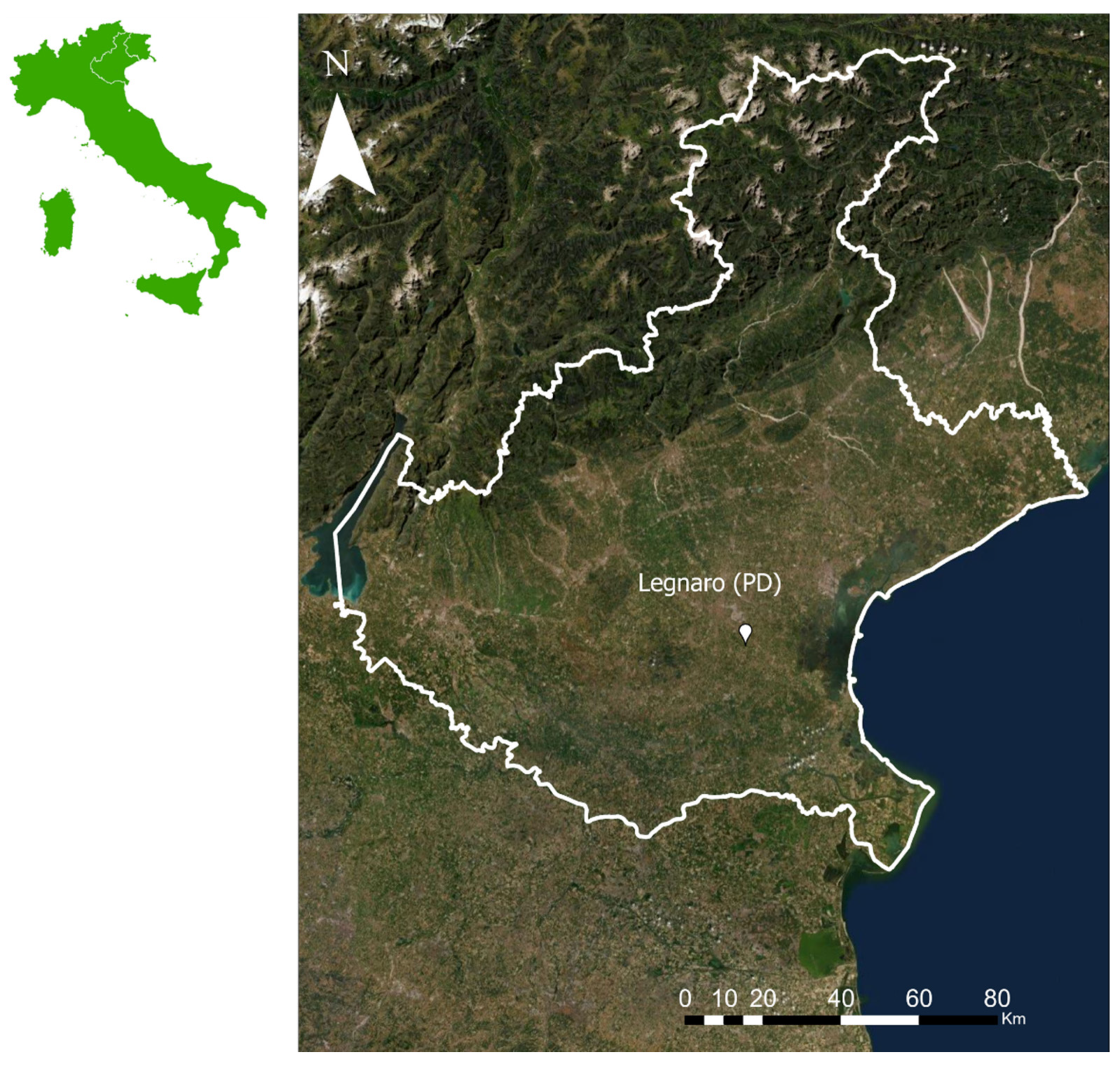
For this study, two different experimental fields were designed; a CV managed field in Pozzoveggiani locality 45°20′38.51″ N 11°54′51.36″ E, and a CA managed field in Legnaro 45°20′49.45″ N 11°57′12.44″ E. Both fields are part of the ‘Lucio Toniolo’ experimental farm of the University of Padua, and both are located in Legnaro, Padua Province, Veneto Region, Italy (
Figure 1).
The surface of both fields is predominantly flat and the soils are classified as Fluvic Cambisols according to the FAO-UNESCO classification, which is common to the Venetian flood plain [
32]. The local climate presents sub-humid traits with an average temperature of 12 °C and approximately 800–850 mm/year of rainfall. Precipitation is mostly concentrated in the autumn and spring, based on data from the Regional Agency for Environmental Protection (ARPA); precipitation for the study period and the locality were also provided by the aforementioned agency, and are presented in
Figure 2.
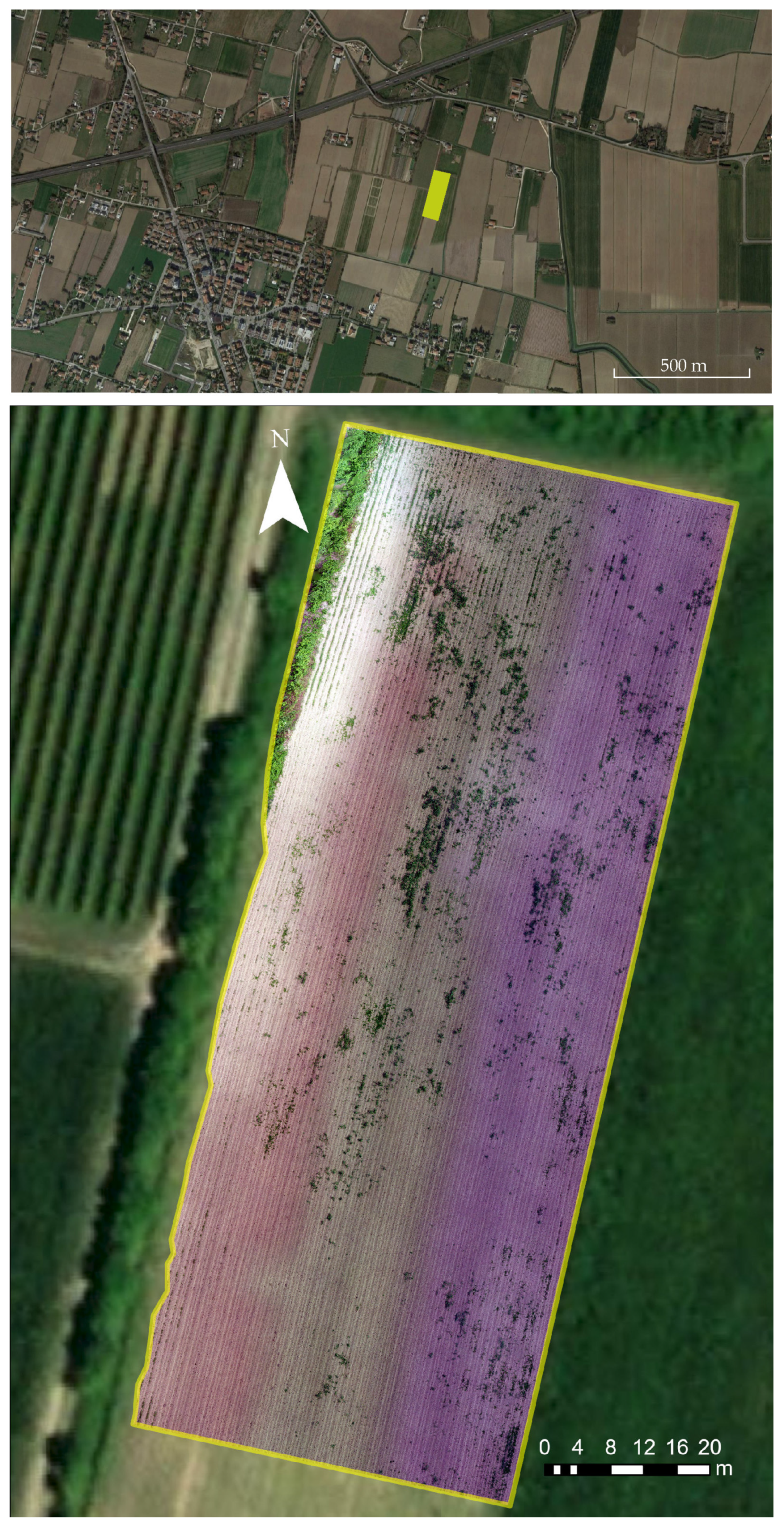
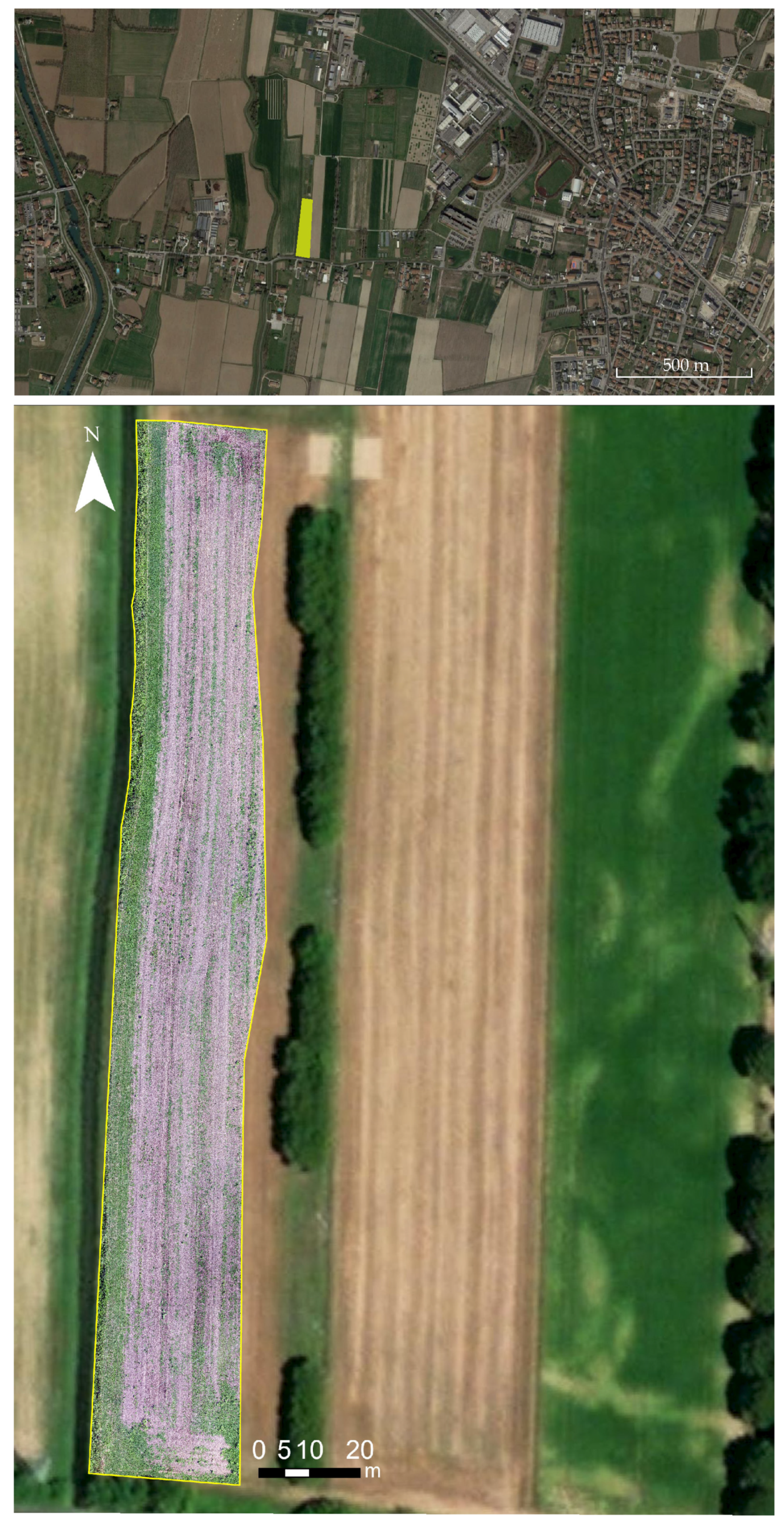
At the Pozzoveggiani field, mechanical measures are applied for soil tillage, while the Legnaro field has been managed under no-till practices since 2014. Specifically, the mechanical measures applied in the CV field were as follows: ploughing on 20th September 2018, and harrowing on 5th and 15th of October 2018, before
Lolium multiflorum was sown. The field was ploughed again on 1st of April 2020 and harrowed on 20th and 24th of April 2020, before soybean was sown. The area of the CV field is 5896.97 m
2, while the area of the CA field is 5643.68 m
2; both fields are represented in
Figure 3 and
Figure 4, respectively.
2.2. UAV Survey
UAV flights were performed twice, in two consecutive years (2019 and 2020), for both fields, for a total of four surveys. The UAV surveys were conducted using a DJI Matrice 200, equipped with DJI X5S sensor (21 M pixel CMOS) (DJI Sciences and Technologies Ltd., Shenzhen, China). The flight plan was set at an altitude of 35 m from the ground; image acquisition during the flight was set at 83% frontal and lateral overlap. For the CA field, the first flight was executed on July 30th 2019 and the second on August 10th 2020, both times after the wheat (
Triticum sp.) harvest. For the CV field, the first flight was performed on September 12th 2019 after the harvest of Italian ryegrass (
Lolium multiflorum), and the second on May 29th 2020 before soybean was sown (
Glycine max). For the creation of the orthomosaics, Pix4D
® Mappersoftware (Pix4D S.A., Prilly, Switzerland) was used, providing four different orthophotos at a very high image resolution (2 mm) for further analysis, as can be seen in
Figure 3 and
Figure 4.
2.3. Weed Classification
For weed classification operations SAGA GIS open-source software (version 7.6.2) was used. The classification was performed using the Maximum Likelihood Classification (MLC) algorithm, part of the supervised classification for grids option of the aforementioned program. The MLC was chosen for its ability to discriminate between weeds and the surrounding elements, as indicated by different authors [
33,
34,
35]. MLC is based on two principles: that the cells in each class sample in the multidimensional space are normally distributed, and on the Bayes theorem of decision making. Considering these two principles, for each cell corresponding to a single pixel, statistical probability is computed for each class to determine the association of every single cell to a specific class. The MLC represents a classification in which a pixel with the maximum likelihood is classified into the corresponding class [
36,
37]. The MLC requires a raster file and a sample classification with defined classes as input data, according to which it will produce the maximum likelihood classification [
37,
38]. Two classes were used for classification: weed and non-weed. As only the weed category was of interest for further analysis, the non-weed category was disregarded. When classification was completed, the newly produced classification was imported into the ArcGIS
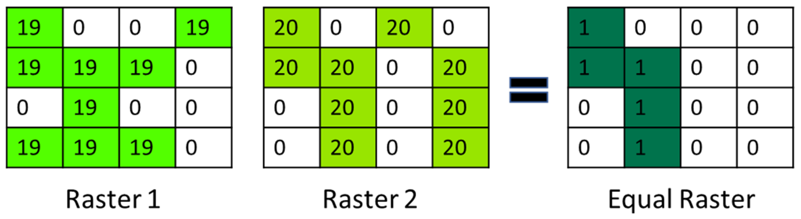
® Pro program (v2.2.0 Environmental Systems Research Institute (ESRI), Redlands, CA, USA) as a raster file. With the help of the raster calculator function (part of the spatial analyst toolbox that allows the creation and execution of map algebra expressions) it was possible to find the same areas in each field in both years by comparing the two raster files from different years. The ‘equal to’ function (==) performs a relational ‘equal to’ operation on two inputs on a cell-by-cell basis, returning 1 for cells where the first raster equals the second raster, and 0 for cells where it does not, as shown in
Figure 5 and Equation (1) [
39].
where Equal Raster contains the pixels that are classified as weeds in both Raster 1 and Raster 2.
Therefore, if the same pixel was classified as weeds in both years (in two raster files), the result will be 1, while if it was classified as weeds in only one year the result will be 0; the order of the raster files is not important. These values in numeric format can be found in the attribute table of the raster files [
39]. After the equal area was determined, it was possible to calculate the percentage of weed distribution difference in the same field comparing two years using a simple Equation (2).
where x represents the percentage of area that was covered with weeds in both years, a is the area that was defined as equal, and b is the total area covered with weeds in the second year.
3. Results
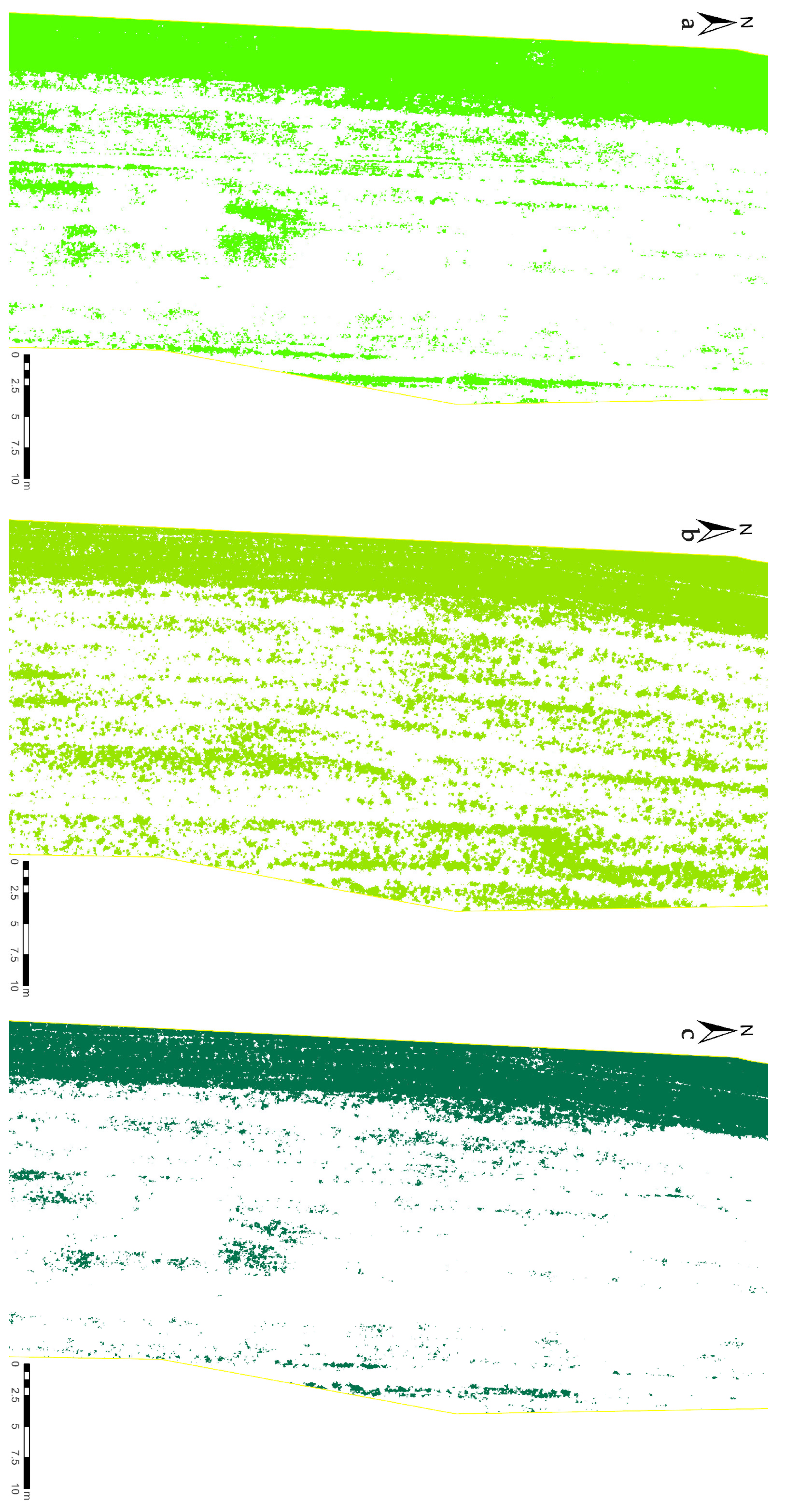
Weed presence differed between the CA and the CV fields; the CA field under no-till management was more infested. Weed presence in the CA field in 2019, 2020, and in both years is shown in
Figure 6.
In 2019, the infested area of the CA field, including field margins, was 159 m2, while in 2020 that area grew to 227.73 m2. The overlapping area (infested in both years) is equal to 127.94 m2, which corresponds to 56.18% of the infested area from 2020. Therefore, it seems that in addition to expanding, in 2020 weeds colonized areas that were not infested in 2019, while some areas that were infested in 2019 were weed free in 2020.
In terms of cardinal directions, in 2019 the infestation was mainly concentrated along the western sector, due to the presence of the field margin; other weed areas are localized in the central and southern sector of the parcel (
Figure 6a). The northern and eastern sectors of the field were much less infested. In 2020, the infestation appears to remain stable in the previously infested regions; however, it heterogeneously increased in the eastern and northern sectors (
Figure 6b).
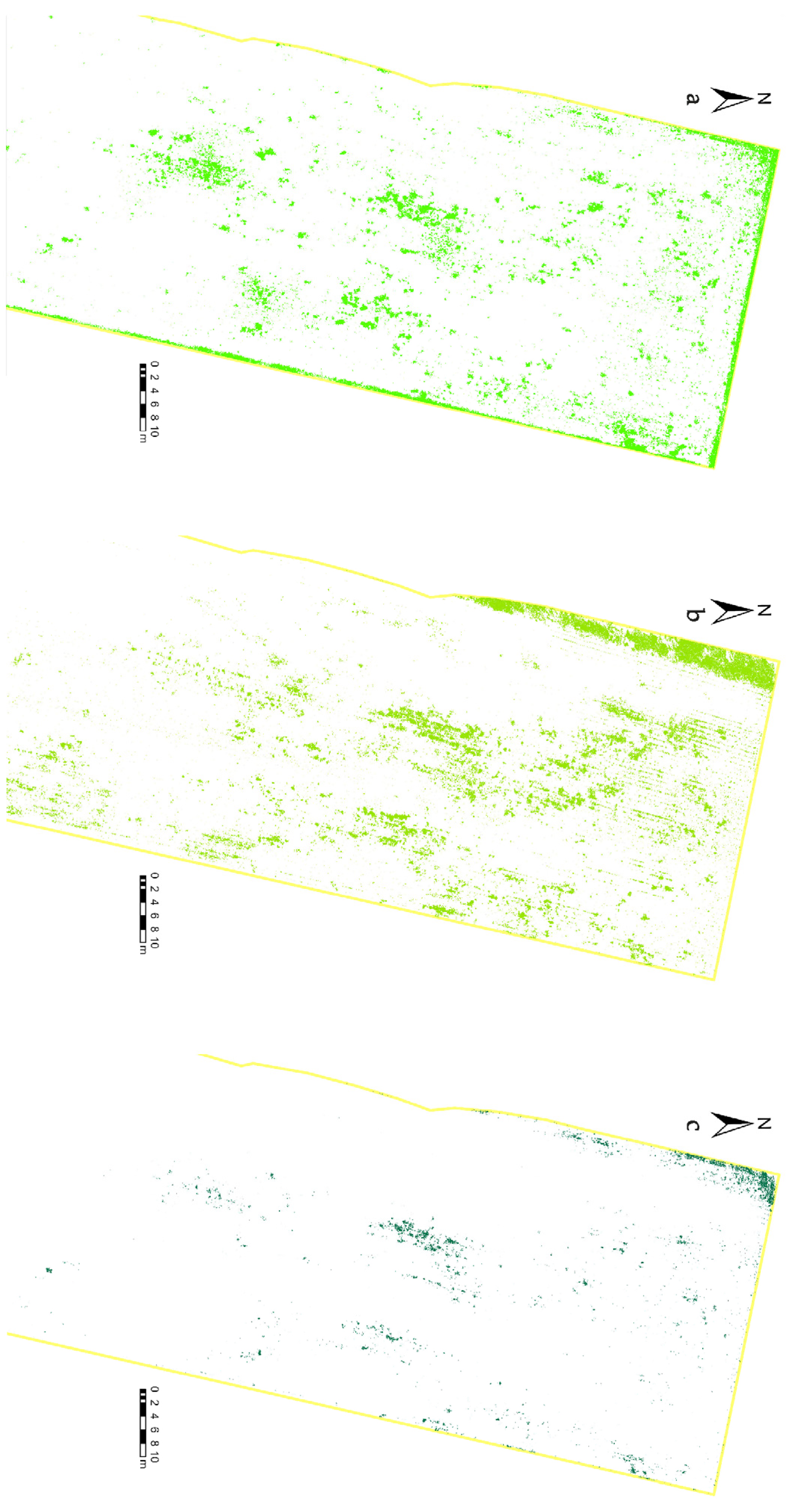
The infested area of the CV field is represented in
Figure 7.
Moreover, an increment of the infested area can also be observed between years, as in the CA field. In 2019, the infested area occupied 63.1 m2, while in 2020, the area was 77.53 m2. On the other hand, the area infested in both years was only 8.92 m2, corresponding to 11.50% of the infested area from 2020. In main cardinal terms the CV field was mostly infested in the northern, central, and eastern sectors, while the southern and western sectors were less infested. In 2020, the infestation shifted more to the south and west of the field, probably as a result of tillage operations.
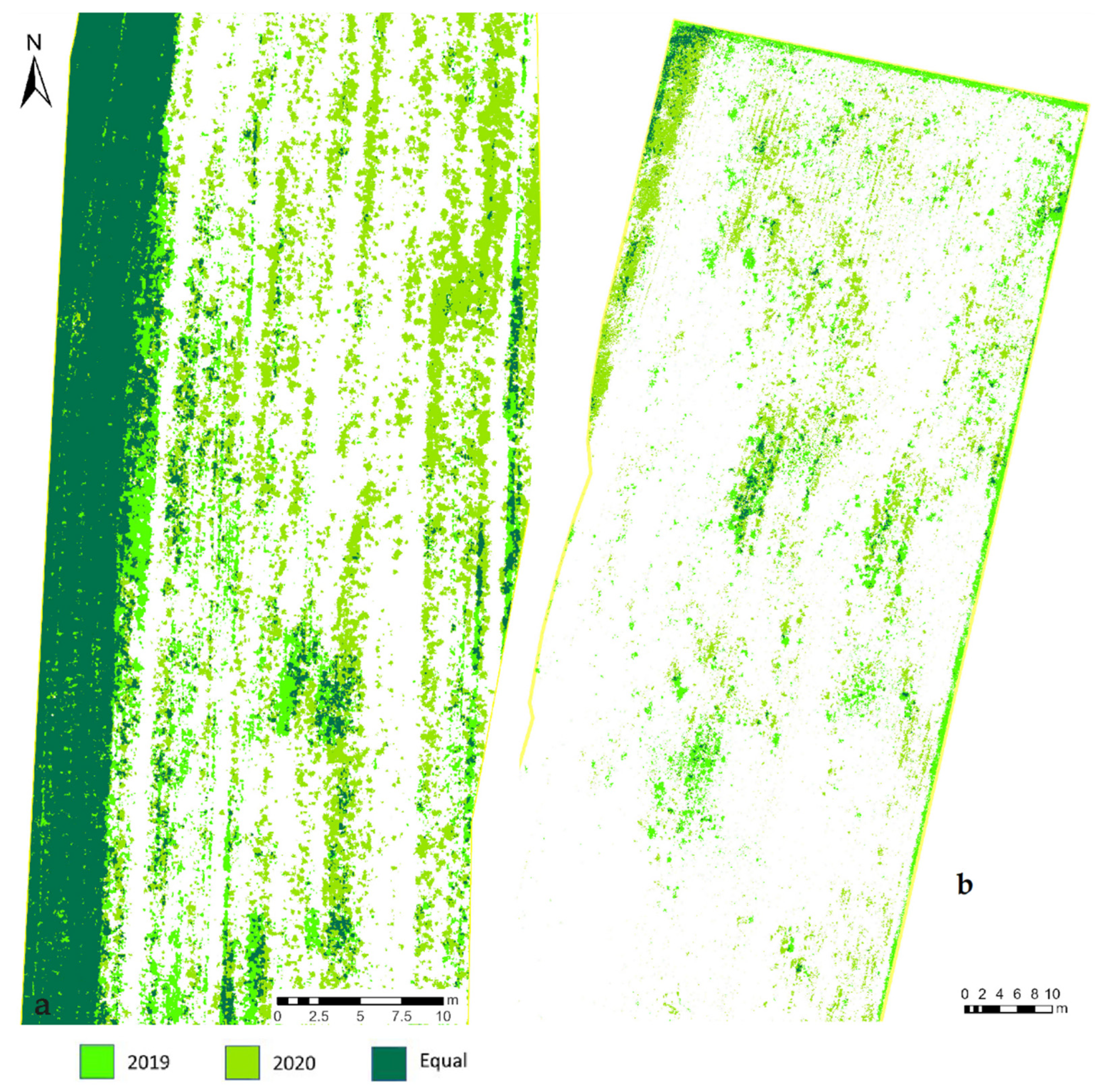
Therefore, the results indicate important differences in weed distribution change between CV and CA managed fields, as shown in
Figure 8.
As shown in
Figure 8, the percentage of area that was infested in both years is higher in the CA field (56.18%) than in the CV field (11.50%).
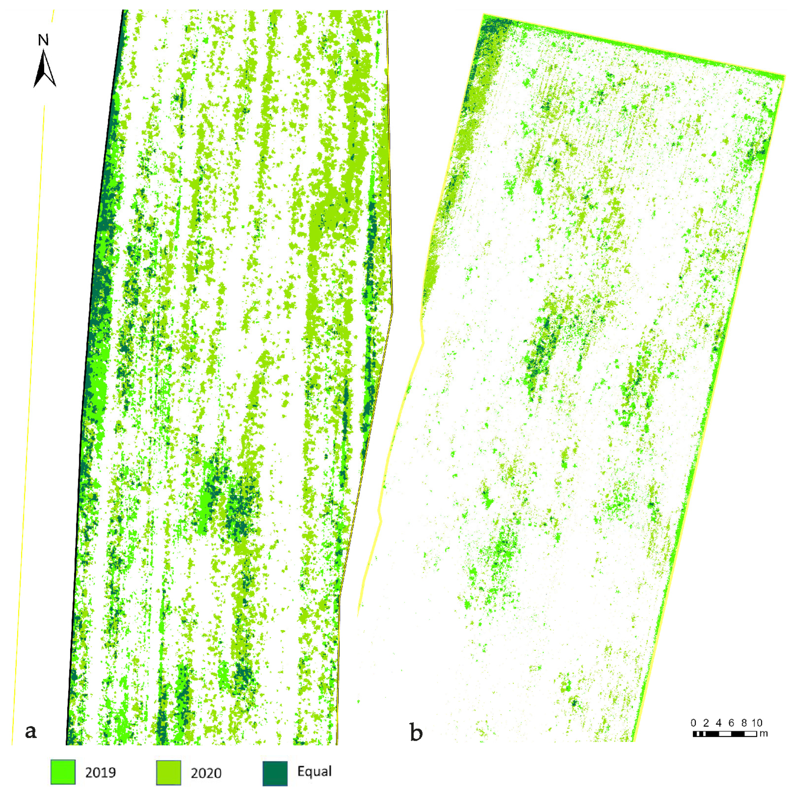
Removing the area near the CA field margin infestation drastically changed the percentages of infestation, as shown in
Figure 9.
Excluding the field margin, the infested area in 2019 occupied 57.55 m2, instead of 159 m2 with field margin included. In 2020, the infested area excluding the field margin was greater than in 2019, reaching 128.29 m2 (227.73 m2 with field margin included). These results highlight the influence of the field margin on the weed infestation of no-till fields, and point out the necessity to pay attention to its management.
Excluding the field margin of the CA field, the area infested in both years was 28.90 m2 that corresponded to 22.53% with respect to 127.94 m2 that corresponded to 56.18% with the field margin.
Even though the area infested in both years was reduced by excluding the field margin effect of the no-till management field, in
Figure 10 it can be seen that the CA field area infested in both years is still higher than that of the CV field. Indeed, excluding the field margin, the area infested in both years in the CA field was almost twice that of the CV field.
4. Discussion
Limited information about tracking the change in weed distribution comparing differently managed fields is documented in the literature, especially considering that most of the research is based on tracking invasive weed species’ distribution change, which may have severe implications on human lives and agricultural production under the changing climate [
40,
41,
42]. Yet both in Europe and globally, there is a rising trend in the use of modern technologies that are becoming ever more available and user-friendly to support precision agriculture, including weed monitoring for precision weed control [
43]. Therefore, these technologies can be used in a rather simple but reliable way, to detect spatial changes in time in different field management systems, offering both scientific and practical information for decision-makers. The results obtained were expected; they are in accordance with what is known about the influence of soil management on the distribution of reproductive plant material [
44,
45,
46].
Moreover, the two fields differ in weed species composition. While in the CV field the weed community mainly consists of
Sorghum halepense and
Abutilon theophrasti, in the CA field, there was a higher species richness consisting of
Digitaria sanguinalis,
Abutilon theophrasti,
Amaranthus retroflexus,
Chenopodium album, and small amounts of several other species. In contrast, the field margin was heavily populated with
Sorghum halepense. This finding is in accordance with several studies indicating that no-till systems often have richer weed species communities compared to CV managed fields [
47,
48,
49]. This difference in weed species richness could be one of the reasons for different field infestations between CV and CA fields; weeds can easily proliferate considering the abundance of precipitation during the study period. Moreover, the presence of an irrigation canal in the CA field is probably responsible for a highly developed field margin.
Still, the use of UAVs for weed detection in different agricultural systems is well known [
28,
50,
51], as is the use of different algorithms, including MLC, that can recognize weed patches with a high degree of accuracy, enabling better weed control strategies [
52,
53,
54]. Therefore, the results obtained by the approach used in this study indicates that UAVs and detection algorithms can be valuable tools for tracking weed distribution changes, even considering the specific realities of different cropping systems. Furthermore, in the future or in areas where experimentation is permitted, these maps could be used for aerial spraying weed control operations performed using a UAV [
55] to indicate the areas more at risk of infestation.
Lastly, the edges of the fields are often observed to have a higher density of weed infestation than the more central areas of the fields [
56]. This was particularly evident in the no-till field. This result is apparently related to a reduction in agricultural inputs near the field borders and/or the dissemination of weeds from the ditch and the surrounding landscape. This was very well observed in the CA field by the methods used in this study, and it strongly influenced the results. Since the field margin is considered a ruderal site and is managed differently compared to the field, good identification of the field margin obtained using the image analysis allowed its exclusion from further analysis. The comparison was repeated without considering the area of the CA field margin in order to include only the weed distribution data from the arable area.
5. Conclusions
The results obtained showed that the methodology for tracking weed spatial changes in time, as proposed in this paper, can be a reliable and very useful tool. Indeed, using the UAV and the identification algorithms it was possible to deduce the level of stability of weed patches over time in the fields under different management systems. Furthermore, the simplicity of this approach should allow stakeholders and decision-makers to apply it with minimal training. The results also point out the evident differences between spatial distribution in fields under different management conditions over time. While constant mechanical operations in the CV field seem to directly influence the seedbank and the transport of reproductive plant material across the field, those elements are not present or are severely reduced in the no-till system. Seeds disseminated or introduced in the fields under different agricultural systems experience different conditions, affecting their spatial distribution, germination, emergence, and longevity. Some of these specific conditions are the lack of seed burial and the permanent residual soil cover in the CA field, which are not present in the CV field. Considering that precision weed control using site-specific methods is already applied both in CV and in CA, changes in spatial distribution could affect the use of these methods. Considering the low stability of weed patches over time in CV, it would be imperative to perform UAV monitoring surveys every year in order to identify the weed patches for satisfactory site-specific weed control. However, if spatial aggregation for many weed species persists from year to year in no-till systems, maps made in one year could be used as a point of reference for precision weed control in the following years. Indeed, considering that weed patches in CA remain more stable, those specific areas of the field are quite suitable for weed development. In those places, weed–crop competition will be higher, resulting in severe yield loss. Therefore, it might be possible to have satisfactory weed control results in CA fields without the need to perform UAV surveys every year. Results obtained in this experiment also highlight another important issue of CA fields: the field margins. The influence of field margins on field infestation can be quite high; therefore, it is important to dedicate more attention to weed control practices applied close to the margin.
Further research is needed, including long term studies on many fields with different weed communities, to better understand changes in weed distribution over time and in different climatic conditions. Moreover, the temporal stability of patch distribution studies should consider species-specific behavior and also the influence of field margins. For all these possible future research studies, the methods described in this study provide an easy and highly precise solution.
Author Contributions
Conceptualization, N.N., R.M. and S.E.P.; methodology, N.N.; software, N.N.; validation, N.N., P.M. and S.E.P.; formal analysis, N.N.; investigation, N.N., P.M., S.E.P. and C.M.; resources, C.M., P.M., S.E.P., N.N., R.M. and M.D.M.; data curation, N.N. and C.M.; writing—original draft preparation, N.N.; writing—review and editing, R.M., S.E.P., P.M. and M.D.M.; visualization, N.N., P.M. and S.E.P.; supervision, R.M., S.E.P. and M.D.M. All authors have read and agreed to the published version of the manuscript.
Funding
Advanced Master in GIScience and Unmanned Aerial Vehicles, ICEA Department, University of Padua.
Data Availability Statement
Not applicable.
Acknowledgments
We would like to thank Archetipo s.r.l. for supporting UAV surveys in experimental research.
Conflicts of Interest
The authors declare no conflict of interest.
References
- Swanton, C.J.; Harker, K.N.; Anderson, R.L. Crop Losses Due to Weeds in Canada. Weed Technol. 1993, 7, 537–542. [Google Scholar] [CrossRef]
- Gharde, Y.; Singh, P.K.; Dubey, R.P.; Gupta, P.K. Assessment of yield and economic losses in agriculture due to weeds in India. Crop Prot. 2018, 107, 12–18. [Google Scholar] [CrossRef]
- Milberg, P.; Hallgren, E. Yield loss due to weeds in cereals and its large-scale variability in Sweden. Field Crop Res. 2004, 86, 199–209. [Google Scholar] [CrossRef]
- Oerke, E.C. Crop losses to pests. J. Agric. Sci. 2006, 144, 31–43. [Google Scholar] [CrossRef]
- Dekker, J. Soil weed seed banks and weed management. J. Crop Prod. 1999, 2, 139–166. [Google Scholar] [CrossRef]
- Skroch, W.A.; Dana, M.N. Sources of Weed Infestation in Cranberry Fields. Weeds 1965, 13, 263–267. [Google Scholar] [CrossRef]
- Dastgheib, F. Relative importance of crop seed, manure and irrigation water as sources of weed infestation. Weed Res. 1989, 29, 113–116. [Google Scholar] [CrossRef]
- Snir, A.; Nadel, D.; Groman-Yaroslavski, I.; Melamed, Y.; Sternberg, M.; Bar-Yosef, O.; Weiss, E. The origin of cultivation and proto-weeds, long before neolithic farming. PLoS ONE 2015, 10, e0131422. [Google Scholar] [CrossRef] [Green Version]
- Thrall, P.H.; Bever, J.D.; Burdon, J.J. Evolutionary change in agriculture: The past, present and future. Evol. Appl. 2010, 3, 405–408. [Google Scholar] [CrossRef]
- Dekker, J. Weed Diversity and Weed Management. Weed Sci. 1997, 45, 357–363. [Google Scholar] [CrossRef]
- Peters, K.; Breitsameter, L.; Gerowitt, B. Impact of climate change on weeds in agriculture: A review. Agron. Sustain. Dev. 2014, 34, 707–721. [Google Scholar] [CrossRef] [Green Version]
- Ramesh, K.; Matloob, A.; Aslam, F.; Florentine, S.K.; Chauhan, B.S. Weeds in a changing climate: Vulnerabilities, consequences, and implications for future weed management. Front. Plant Sci. 2017, 8, 1–12. [Google Scholar] [CrossRef] [PubMed]
- Ziska, L.H. Elevated carbon dioxide alters chemical management of Canada thistle in no-till soybean. Field Crop Res. 2010, 119, 299–303. [Google Scholar] [CrossRef]
- Sun, Y.; Ding, J.; Siemann, E.; Keller, S.R. Biocontrol of invasive weeds under climate change: Progress, challenges and management implications. Curr. Opin. Insect Sci. 2020, 38, 72–78. [Google Scholar] [CrossRef] [PubMed]
- Arriaga, F.J.; Guzman, J.; Lowery, B. Conventional Agricultural Production Systems and Soil Functions. In Soil Health and Intensification of Agroecosytems; Elsevier: Amsterdam, The Netherlands, 2017; pp. 109–125. ISBN 9780128054017. [Google Scholar]
- FAO Conservation Agriculture. Available online: http://www.fao.org/conservation-agriculture/en/ (accessed on 29 March 2022).
- Bullied, W.J.; Marginet, A.M.; Van Acker, R.C. Conventional- and conservation-tillage systems influence emergence periodicity of annual weed species in canola. Weed Sci. 2003, 51, 886–897. [Google Scholar] [CrossRef]
- Pardo, G.; Cirujeda, A.; Perea, F.T.; Verdù, A.M.C.; Mas, M.T.; Urbano, J.M. Effects of reduced and conventional tillage on weed communities: Results of a long-term experiment in southwestern spain. Planta Daninha 2019, 37, 1–12. [Google Scholar] [CrossRef]
- Radosevich, S.R.; Holt, J.S.; Ghersa, C.; Radosevich, S.R. Ecology of Weeds and Invasive Plants: Relationship to Agriculture and Natural Resource Management; Wiley-Interscience: Hoboken, NJ, USA, 2007; ISBN 0470168935. [Google Scholar]
- Zimdahl, L.R. Fundamentals of Weed Science, 3rd ed.; Elsevier: Amsterdam, The Netherlands, 2007; ISBN 9780080549859. [Google Scholar]
- Nichols, V.; Verhulst, N.; Cox, R.; Govaerts, B. Weed dynamics and conservation agriculture principles: A review. Field Crop. Res. 2015, 183, 56–68. [Google Scholar] [CrossRef] [Green Version]
- Petit, S.; Alignier, A.; Colbach, N.; Joannon, A.; Cœur, D.; Thenail, C. Weed dispersal by farming at various spatial scales. A review. Agron. Sustain. Dev. 2013, 33, 205–217. [Google Scholar] [CrossRef]
- Sanaullah, M.; Usman, M.; Wakeel, A.; Cheema, S.A.; Ashraf, I.; Farooq, M. Terrestrial ecosystem functioning affected by agricultural management systems: A review. Soil Tillage Res. 2020, 196, 104464. [Google Scholar] [CrossRef]
- Kritikos, M. Precision Agriculture in Europe: Legal, Social and Ethical Considerations; European Parliamentary Research Service, European Parliament: Strasbourg, France, 2017; ISBN 9789282368855. [Google Scholar]
- Tsouros, D.C.; Bibi, S.; Sarigiannidis, P.G. A review on UAV-based applications for precision agriculture. Information 2019, 10, 349. [Google Scholar] [CrossRef] [Green Version]
- Lambert, J.P.T.; Hicks, H.L.; Childs, D.Z.; Freckleton, R.P. Evaluating the potential of Unmanned Aerial Systems for mapping weeds at field scales: A case study with Alopecurus myosuroides. Weed Res. 2018, 58, 35–45. [Google Scholar] [CrossRef] [PubMed] [Green Version]
- Koot, T.M. Weed Detection with Unmanned Aerial Vehicles in Agricultural Systems; Wageningen University: Wageningen, The Netherlands, 2014. [Google Scholar]
- Lottes, P.; Khanna, R.; Pfeifer, J.; Siegwart, R.; Stachniss, C. UAV-based crop and weed classification for smart farming. In Proceedings of the 2017 IEEE International Conference on Robotics and Automation (ICRA), Singapore, 29 May–3 June 2017; pp. 3024–3031. [Google Scholar]
- Failla, S.; Pirchio, M.; Sportelli, M.; Frasconi, C.; Fontanelli, M.; Raffaelli, M.; Peruzzi, A. Evolution of smart strategies and machines used for conservative management of herbaceous and horticultural crops in the mediterranean basin: A review. Agronomy 2021, 11, 106. [Google Scholar] [CrossRef]
- Kassam, A.; Friedrich, T.; Derpsch, R.; Kienzle, J. Overview of the Worldwide Spread of Conservation Agriculture. Fact. Rep. 2015, 8, 1–8. [Google Scholar]
- Kassam, A.; Friedrich, T.; Derpsch, R. Global spread of Conservation Agriculture. Int. J. Environ. Stud. 2019, 76, 29–51. [Google Scholar] [CrossRef]
- FAO World Reference Base for Soil Resources. World Soil Resources Report 103; FAO World Reference Base for Soil Resources: Rome, Italy, 2006; Volume 43, ISBN 9251055114. [Google Scholar]
- Sheffield, K.; Dugdale, T. Supporting urban weed biosecurity programs with remote sensing. Remote Sens. 2020, 12, 2007. [Google Scholar] [CrossRef]
- Eddy, P.R.; Smith, A.M.; Hill, B.D.; Peddle, D.R.; Coburn, C.A.; Blackshaw, R.E. Comparison of neural network and maximum likelihood high resolution image classification for weed detection in crops: Applications in precision agriculture. In Proceedings of the 2006 IEEE International Symposium on Geoscience and Remote Sensing, Denver, CO, USA, 31 July–4 August 2006; pp. 116–119. [Google Scholar]
- Asad, M.H.; Bais, A. Weed detection in canola fields using maximum likelihood classification and deep convolutional neural network. Inf. Process. Agric. 2020, 7, 535–545. [Google Scholar] [CrossRef]
- Sun, J.; Yang, J.; Zhang, C.; Yun, W.; Qu, J. Automatic remotely sensed image classification in a grid environment based on the maximum likelihood method. Math. Comput. Model. 2013, 58, 573–581. [Google Scholar] [CrossRef]
- Sisodia, P.S.; Tiwari, V.; Kumar, A. Analysis of Supervised Maximum Likelihood Classification for remote sensing image. In Proceedings of the International Conference on Recent Advances and Innovations in Engineering (ICRAIE-2014), Jaipur, India, 9–11 May 2014; pp. 9–12. [Google Scholar]
- Conrad, O.; Bechtel, B.; Bock, M.; Dietrich, H.; Fischer, E.; Gerlitz, L.; Wehberg, J.; Wichmann, V.; Böhner, J. System for Automated Geoscientific Analyses (SAGA) v. 2.1.4. Geosci. Model Dev. 2015, 8, 1991–2007. [Google Scholar] [CrossRef] [Green Version]
- Esri ArcGis Pro. Available online: https://www.esri.com/en-us/arcgis/products/arcgis-pro/resources (accessed on 1 May 2022).
- Al Ruheili, A.M.; Al Sariri, T.; Al Subhi, A.M. Predicting the potential habitat distribution of parthenium weed (Parthenium hysterophorus) globally and in Oman under projected climate change. J. Saudi Soc. Agric. Sci. 2022, in press. [Google Scholar] [CrossRef]
- Adhikari, A.; Rew, L.J.; Mainali, K.P.; Adhikari, S.; Maxwell, B.D. Correction to: Future distribution of invasive weed species across the major road network in the state of Montana, USA. Reg. Environ. Chang. 2020, 20, 1–14. [Google Scholar] [CrossRef]
- Wirngo, M.H.; Moise, M.; Ndzeidze, S.K. Mapping and Monitoring Invasive Weeds in the Savannah Grasslands of Western Highlands in Cameroon. Int. J. Ecosyst. 2021, 11, 17–29. [Google Scholar]
- Krähmer, H.; Andreasen, C.; Economou-Antonaka, G.; Holec, J.; Kalivas, D.; Kolářová, M.; Novák, R.; Panozzo, S.; Pinke, G.; Salonen, J.; et al. Weed surveys and weed mapping in Europe: State of the art and future tasks. Crop Prot. 2020, 129, 1–13. [Google Scholar] [CrossRef]
- Cardina, J.; Johnson, G.A.; Sparrow, D.H. The Nature and Consequence of Weed Spatial Distribution. Weed Sci. 1997, 45, 364–373. [Google Scholar] [CrossRef]
- Izquierdo, J.; Blanco-Moreno, J.M.; Chamorro, L.; González-Andújar, J.L.; Sans, F.X. Spatial distribution of weed diversity within a cereal field. Agron. Sustain. Dev. 2009, 29, 491–496. [Google Scholar] [CrossRef]
- Garibay Salvador, V.; Walter, R.; Peter, S.; Tomomi, N.; Junko, Y.; Cyrus, A.; Edwards Peter, J. Extent and implications of weed spatial variability in arable crop fields. Plant Prod. Sci. 2001, 4, 259–269. [Google Scholar] [CrossRef] [Green Version]
- Shahzad, M.; Farooq, M.; Hussain, M. Weed spectrum in different wheat-based cropping systems under conservation and conventional tillage practices in Punjab, Pakistan. Soil Tillage Res. 2016, 163, 71–79. [Google Scholar] [CrossRef]
- Travlos, I.S.; Cheimona, N.; Roussis, I.; Bilalis, D.J. Weed-species abundance and diversity indices in relation to tillage systems and fertilization. Front. Environ. Sci. 2018, 6, 1–10. [Google Scholar] [CrossRef] [Green Version]
- Menalled, F.D.; Gross, K.L.; Hammond, M. Weed aboveground and seedbank community responses to agricultural management systems. Ecol. Appl. 2001, 11, 1586–1601. [Google Scholar] [CrossRef]
- Tamouridou, A.A.; Alexandridis, T.K.; Pantazi, X.E.; Lagopodi, A.L.; Kashefi, J.; Moshou, D. Evaluation of UAV imagery for mapping Silybum marianum weed patches. Int. J. Remote Sens. 2017, 38, 2246–2259. [Google Scholar] [CrossRef]
- Torres-Sánchez, J.; Peña, J.M.; de Castro, A.I.; López-Granados, F. Multi-temporal mapping of the vegetation fraction in early-season wheat fields using images from UAV. Comput. Electron. Agric. 2014, 103, 104–113. [Google Scholar] [CrossRef]
- Perez-Ortiz, M.; Gutierrez, P.A.; Pena, J.M.; Torres-Sanchez, J.; Lopez-Granados, F.; Hervas-Martinez, C. Machine learning paradigms for weed mapping via unmanned aerial vehicles. In Proceedings of the 2016 IEEE Symposium Series on Computational Intelligence (SSCI), Athens, Greece, 6–9 December 2017. [Google Scholar]
- Mattivi, P.; Pappalardo, S.E.; Nikolić, N.; Mandolesi, L.; Persichetti, A.; De Marchi, M.; Masin, R. Can commercial low-cost drones and open-source gis technologies be suitable for semi-automatic weed mapping for smart farming? A case study in ne italy. Remote Sens. 2021, 13, 1869. [Google Scholar] [CrossRef]
- Nikolić, N.; Rizzo, D.; Marraccini, E.; Ayerdi Gotor, A.; Mattivi, P.; Saulet, P.; Persichetti, A.; Masin, R. Site and time-specific early weed control is able to reduce herbicide use in maize—A case study. Ital. J. Agron. 2021, 16. [Google Scholar] [CrossRef]
- Sarri, D.; Martelloni, L.; Rimediotti, M.; Lisci, R.; Lombardo, S.; Vieri, M. Testing a multi-rotor unmanned aerial vehicle for spray application in high slope terraced vineyard. J. Agric. Eng. 2019, 50, 38–47. [Google Scholar] [CrossRef]
- Alignier, A.; Petit, S.; Bohan, D.A. Relative effects of local management and landscape heterogeneity on weed richness, density, biomass and seed rain at the country-wide level, Great Britain. Agric. Ecosyst. Environ. 2017, 246, 12–20. [Google Scholar] [CrossRef]
| Publisher’s Note: MDPI stays neutral with regard to jurisdictional claims in published maps and institutional affiliations. |
© 2022 by the authors. Licensee MDPI, Basel, Switzerland. This article is an open access article distributed under the terms and conditions of the Creative Commons Attribution (CC BY) license (https://creativecommons.org/licenses/by/4.0/).


 ,
, 


