Assessment of Economic Sustainability in the Construction Sector: Evidence from Three Developed Countries (the USA, China, and the UK)

Abstract

The construction sector plays a significant role in contributing to uplifts in economic stability by generating employment and providing standardized social development. Economic sustainability in the construction sector has been less addressed despite its wide applicability in the economy. This study aimed to perform a comparative analysis to determine the application of a circular economy in the construction sector toward economic sustainability, along with its long-term forecasting. A time series analysis was used on the construction sector of the United States of America (USA), China, and the United Kingdom (UK) from 1970 to 2020, by taking into account individual effects to propose a framework with global validity. Statistical analysis was performed to analyze the dependence of the construction sector and determine its short- and long-term contributions. The results revealed that the construction sectors in these countries tend to bounce back to equilibrium in the case of short-term effects; however, the construction sector behaves differently with respect to each sector after experiencing long-term effects. The results show that the explanatory power of the forecasting model (R²) was found to be 0.997, 0.992, and 0.996 for the USA, China, and the UK. Based on the concept of the circular economy, it was concluded that the USA will become a leader in attaining sustainability in construction owing to its ability to recover quickly from shocks, and that the USA will become the largest construction sector in terms of GDP, with a USD 0.3 trillion higher GDP than that of the Chinese sector. Meanwhile, there will be no significant change in the construction GDP of the UK up to the end of 2050. Moreover, the speeds of the construction sector toward equilibrium in the long run in the USA, China, and the UK, and regaining of their original positions, is 0.267%, 1.04%, and 0.41% of their original positions, respectively. This study has a significance in acting as a guideline for introducing economic and environmental sustainability in construction policies, because of the potential of the construction sectors to recover from possible recessions in their respective countries.

1. Introduction

The activities of each economic sector in a country contribute in many ways to the national gross domestic product (GDP). One of these sectors is construction, which has a deciding role in socioeconomic development by providing infrastructures, transport, employment opportunities, energy demand, telecommunications, and investments [1]. The construction sector is one of the most complex and dynamic sectors of the economy. It contributes to the sustainable objectives of the country, including revenue generation, employment opportunities, and social needs; therefore, an analysis of the construction sector’s effect on the GPD is necessary [2]. The role of the construction sector in cumulative GDP was analyzed, and it was found that the sector is greatly affected by a lack of privatization, skilled labor, inaccessible immigration rules, and the influences of bureaucrats [3]. In the early support of the economy, construction has an influential role in its capability to uplift the GDP of the country and is responsible for its modernization because of its role in improving infrastructure [4]. This sector is regarded as the backbone of the country because it influences every level of the economy [5]. It also has the potential to uplift the economy because it does not only include construction projects but also technological and social change, client demands, and the increasing use of every sector in its execution [6]. With the construction sector making use of resources from all other sectors of the economy, it is therefore considered a driving factor toward prosperity in every country [7]. Owing to the importance of the construction sector, its influences have forward and backward linkages with other sectors. Any negative change in its performance will produce a recession in the economy [8].

For example, in 2018, construction activities in Turkey decreased by 4.8% due to high-interest rates on construction activities and, as a result, the country suffered major losses in the construction sector [9].

Table 1. Construction output of developed countries for 2018–2019.

Country	Value Added in Construction (Current Price, Trillion USD)		Percent Change in Construction (Current Price, Trillion USD)		People Employed in Construction (Millions)	Reference
	2018	2019	2018	2019
Japan	0.281	0.284	1.33%	1.31%	2.93	[10]
Canada	0.126	0.126	3.78%	0.34%	1.20	[11]
Germany	0.175	0.186	12.27%	6.59%	2.13	[12]
France	0.138	0.139	8.55%	0.46%	1.51	[13]
Italy	0.079	0.076	6.15%	−3.38%	1.33	[14]
Australia	0.144	0.142	1.62%	−1.41%	1.10	[15]
Finland	0.017	0.017	11.87%	−1.75%	1.83	[16]
UK	0.123	0.129	3.05%	5.28%	2.30	[17]
USA	0.848	0.892	6.32%	5.25%	9.08	[18]

presents the values of construction and percentage change in various developed countries in 2018–2019 and the corresponding employment levels.

1.1. Construction Sector in the USA, China, and the UK

The construction sector of the United States of America (USA) is regarded as one of the largest marketplaces all over the world [19]. Through its linkages, the US construction sector supports investments, transportation, manufacturing, growth, output, and other related building material industries; moreover, it provides jobs to plenty of workers, which generate income opportunities and reduce poverty [20]. The job losses in workers of all classes in the sector increased toward the end of the first quarter of 2020, and then decreased toward the end of all the remaining quarters of 2020 [21].

In the United Kingdom (UK), the construction sector likewise contributes considerably to the national economy. The UK construction sector has a diverse range of sectors, such as manufacturing, mining, and services. Considered one of the largest sectors of the UK, construction employed over 9% of the workforce in 2019 [22]. The construction sector contributes an estimated 15.3% to the national GDP of the UK and has an economic generation of 6% [23]. 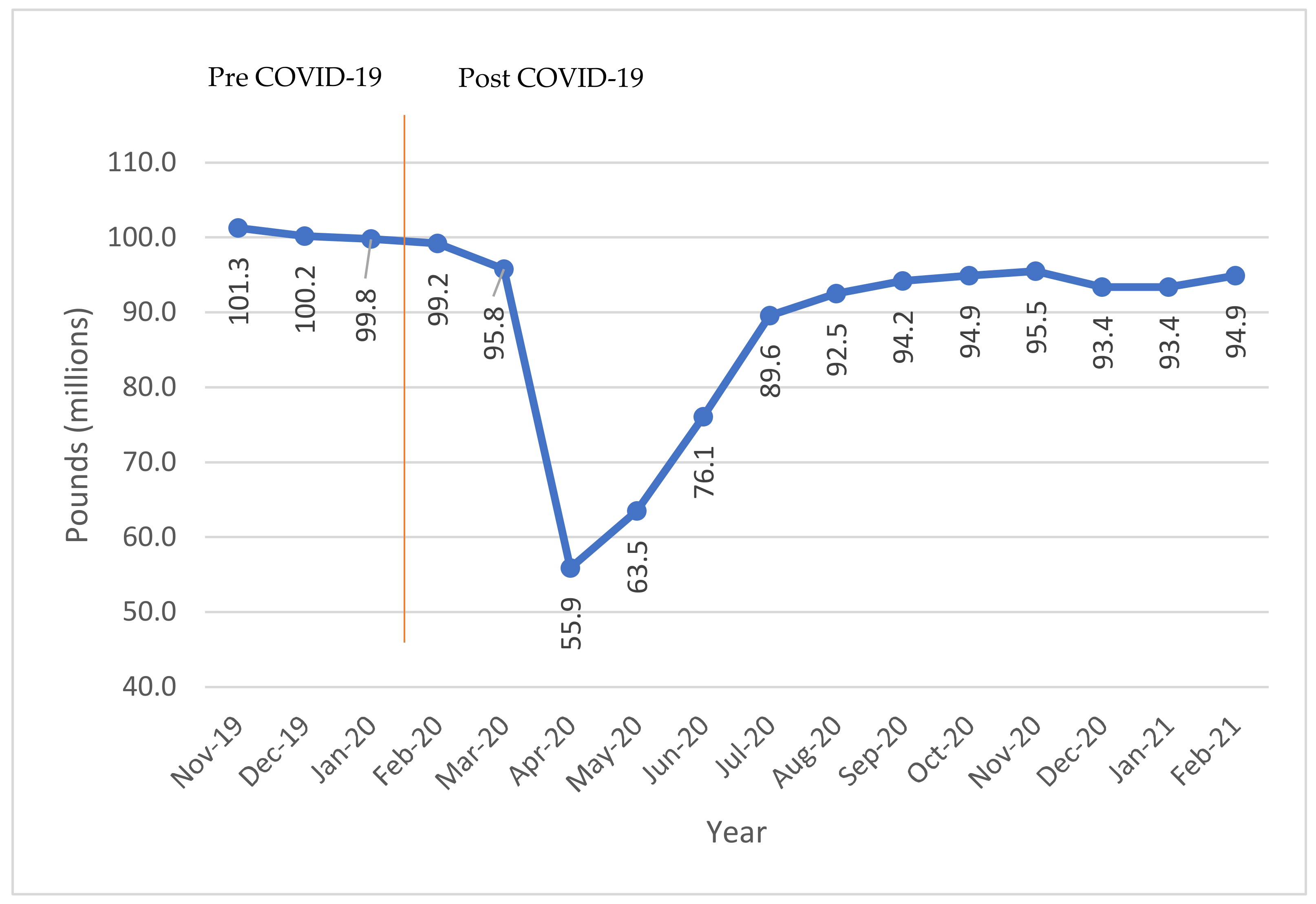Furthermore, it employs 2.3 million people, which is 7.1% of the entire UK workforce, because the average wages of construction sector workers are 5% higher than those of workers in other sectors [24]. With the UK construction sector immensely affected by the COVID-19 crisis, its construction output contracted 19.5% in the first half of 2020 [25].

Figure 1 illustrates the effects of the unseen event on construction sector output in the UK. The growth of construction output was highest in pre-COVID-19 times. However, after COVID-19, the level of construction output decreased up to the end of March 2020 [26].

China is regarded as one of the largest construction output sectors globally with a construction growth of USD 1.04 trillion in 2020 [27]. The sector accounts for a 6.9% contribution to the national GDP of China [28]. In China, the construction industry is fully dependent on materials and services from other sectors that make up the construction workflow in its 30 provinces [29]. Construction activities stopped due to the COVID-19 crisis, which greatly affected the output in the first quarter of 2020 [30]. According to the National Bureau of Statistics, in the Chinese construction industry, there was also a 3.5% growth in the sector in Q4 of 2020, with a growth of 6.6% year on year in the same quarter [31].

Based on construction development trends, it is evident that the construction industry causes the country’s economy to thrive but, on the other hand, it is also the main source of adverse effects to the environment and human existence because of carbon emissions. For example, the current use of resources in the construction sector is problematic, as energy-related CO₂ emissions soared by 9.95 gigatons in 2019, a figure that comprises approximately 38% of global greenhouse gas (GHG) emissions [32]. Therefore, there is a need for a concept that could incorporate the fundamentals of sustainability by minimizing waste products and increasing the efficiency of materials. One such concept is the circular economy.

1.2. Circular Economy

The concept of the circular economy is not new. It was first introduced by Kenneth. E. Boulding in the book The Economics of Natural Resources [33]. The concept is a type of economic development that takes into account the scarcity of materials and its effects on the environment and social aspects [34]. The circular economy addresses three main points, namely, reducing the use of raw materials, recycling demolished materials, and generating less waste debris, thereby reducing environmental pollution and achieving cleaner production [35]. It has been shown that sustainability and the circular economy are related to at least eight relationships [36]. Hence, the innovative aspects of sustainable development need to be introduced into the circular economy in every sector [37]. Circular construction framework techniques will lead to the minimal use of locally available resources, water and energy, less waste generation, and guarantee the reuse and recycling of demolished materials. By reducing the negative impacts on the environment, such a circular framework will pave the way for cleaner construction practices [38]. This study introduces the cleaner circular model for construction practices that can drive countries toward a sustainable construction sector.

This study shows how circularity could be embedded in the construction sector across the globe. The construction sector is the most daunting as it the most unresolved sector with regard to circularity, with a potential for sustainability in terms of the economy and the environment. Meanwhile, investing in the construction sector will ensure its adoption and the invention of sustainable techniques that will ensure sustainability in the economy and construction practices [39]. First, the sector has many kinds of problematic effects on health, the resilience of our communities, and equality. Second, the current rate of change—or even the direction of change—in the construction sector is inadequate, owing to several issues, which have increasingly negative effects on social barriers and social resistance [40]. As an example, carbon emissions were tracked using time series data and carbon indicators were identified to set targets to reach the carbon reduction targets [41], which shows the potential of using time series in achieving sustainability. Hence, the increasing popularity of the circular economy concept means it is starting to be accepted as a coherent strategy to respond to the resource-related and environmental challenges in front of us.

Based on the importance of the influence of the construction (CONST) sector on the national GDP and its role in the road to sustainability, the following research questions, shown in

Table 2. Research questions and their hypothesis.

Research Objective	Research Question	Research Hypothesis
1	How would the cumulative economy of developed countries, such as the USA, China, and the UK, react when an external shock is experienced in the CONST sector?	A shock to the CONST sector does not affect the cumulative economy.
2	In which direction must the CONST sector move to ensure economic sustainability?	Sustainability in the CONST sector is impossible after recovering from the shock.
3	What steps should investors and policy makers take to impose sustainability in the shock-absorbed sector and ensure the sustainable progress of the sector after recovering from the shock?	It is the responsibility of the government rather than the investors and policy makers to drive the sector toward a sustainable economy.
4	What concrete actions should be followed for the application of statistical circularity in the CONST sector?	Time series cannot be used for data analysis in sustainability.

, were established.

The objective of this study is to assess the direction of the construction sector after a shock (e.g., recession or pandemic) has been received in three different countries, namely, the USA, the UK, and China, and how much time the sector will require to move toward economic sustainability. The criteria to determine economic sustainability include environmentally friendly processes, profitability, and social inclusion [42]. The significance of this study is that it will enable policy makers to comprehend the underlying concepts behind the short- and long-term effects of the construction sector and the need for collaboration among investors, to work in closer partnership with innovators to create sustainable economies and generate employment opportunities.

2. Literature Review

The Turkish construction industry has a positive influence on GDP growth. The net GDP of the country increased to 7.3% in 1987 and 11.1% from 2002–2012; this increase was twice the national GDP of the country, which also increased due to the exponential growth in the construction sector [43]. A very important question was analyzed: “Does construction output contribute to economic growth?” It was found that bidirectional linkages exist between the construction sector and the economy of the country, and a positive relationship exists between the short- and long-run effects [44]. The Malaysian construction industry experienced a considerable rise in the construction sector due to the use of highly mechanized modern equipment, which increased construction growth. Residential and non-residential growth increased by 30% and 17.8%, respectively. The productivity indicators showed a rise in the GDP of the economy [45]. Time-series data from 1990 to 2009 were collected in Nigeria. The results revealed that GDP and the construction sector have bidirectional Granger causality, meaning that any change in one sector will affect the performance of other sectors. Hence, the construction sector plays a vital role in contributing to the national economy [46]. Based on the time series of Hong Kong data from 1983 to 2013, a bidirectional correlation in the long-run effect was found between GDP and the construction sector. The long-term linkages suggest that policies, industrial development, and innovation must be introduced in the construction sector to ensure consistent growth [47]. A similar study was conducted in Ghana using data collected from 1968 to 2004. The results revealed that construction growth was linked to overall GDP performance with a three-year lag. Moreover, Ghana’s GDP showed high performance after two years of growth in the construction sector, confirming the causality between construction and GDP [48]. In another study, 50-year period data from 1968 to 2017 were selected to examine an economic shock and its effects on the construction industry. The construction industry was found to have thrived when there was political stability, optimum weather conditions, and less energy shortage. During the military dictatorship, there was a decline of 21.6% in the construction industry [49]. According to a survey conducted in Afghanistan, 25% of construction projects employed 0.5% of the labor workforce and contributed 0.5% to the national economy [50]. Turkey’s construction industry was analyzed based on a data sample from 1998 to 2014. The industry was found to have short-term effects that lasted for just five years on real GDP [51].

2.1. Use of Granger and VECM

In another study, the results showed that construction is a Granger cause of GDP growth and mortgages. It was concluded that these two factors can be used as early indicators for construction performance [52]. A similar study was conducted on statistical data from Malaysia from 1970 to 2019 to study construction sector effects. An impulse response function (IRF) and a vector error correction model (VECM) were used to study shock behavior for short- and long-term effects on the Malaysian economy. A sustainability framework with a global application was also proposed [53]. The need for a post-epidemic prevention system must be integrated to make the construction sector resilient. A standard procedure must be developed that can balance the cost of halted activities in the sector and the probability of a disaster occurring. For this purpose, digital innovation must be employed in the sector to satisfy the need for sustainability [54]. To define the circular economy, a mathematical approach was used that takes into account the recycling of demolition waste for the construction sector in the UK. It was found that government policies could be the only solution to achieving circularity in the construction built environment [55]. An investigative study was performed in Hong Kong to answer the question of which factors are hurdles in adopting cleaner and sustainable processes in the construction sector. From over 140 construction site interviews, the adoption of sustainable processes was found to be greatly related to financial profitability, managerial decisions, and regulatory bodies [56].

2.2. Sustainable Process

The factors contributing to the application of sustainable processes in construction management were reviewed. Based on the interviews, a total of 82 indicators were selected that could relate to the application of cleaner practices in the construction sector. These indicators belong to the areas of social interaction, economic strategies, and environmental processes [57]. To reduce CO₂ emissions, two approaches, namely, production-based and consumption-based, were used to assess global construction carbon emissions. Based on the data from 1995 to 2009, the forward linkage of global construction with CO₂ emissions was found to be between 16% and 20% while the backward linkage was between 37% and 46%. Based on the findings, structural optimization, low-carbon emission processes, and mechanism for transportation were proposed to reduce CO₂ production in the high-pollution sector [58]. In evaluating the number of carbon emissions from the conventional method of construction used in Pakistan, modular CO₂ emissions were found to be 3449.73 kg CO₂-equivalent GHG while conventional building practices generated 6501.91 kg CO₂ GHG emissions. It was concluded that modular construction practices result in 46.9% of CO₂ emissions and must be adopted to achieve sustainability in the system [59]. The waste reduction behavior of construction workers was assessed using a system dynamics approach. Reactive actions and prioritization at the construction site were found to be effective in reducing waste generation. A model based on the policies and measures on the construction site was also proposed to reduce construction waste [60]. An input-output method was adopted to assess the reuse of construction materials. Data from Ontario indicated that reusing construction materials will pose fewer environmental effects and prove beneficial to the economy. It will also increase the GDP and employment opportunities in Canada [61]. To assess the relationship between carbon emissions and the economic prosperity of China’s construction sector, the standard deviational ellipse method was used on data from 2005 to 2015. The carbon emissions of 30 provinces of China were studied, and it was found that the economic development in most provinces has a forward linkage direction with carbon emissions, meaning that low carbon emissions indicate slow economic development in these particular provinces. Therefore, the need for policy making for sustainable development was proposed [62]. Statistical analysis was performed based on a questionnaire survey in the Indian construction sector. It was found that resource policies, eco-friendly practices, industry green technologies, and an institutional framework for the application of sustainability in the construction sector are the driving factors toward attaining sustainability and could prove helpful for policy makers and project managers in the construction sector [63]. The construction sector of China and its neighboring countries were investigated for the linkages between the economy, environment, and resources. Compared to other countries, the construction sector of China generates more carbon emissions. It uses more resources and generates more emissions compared to economic profit for the countries in which Chinese firms utilize energy. Based on such findings, protective measures such as energy structure, practices for sustainable development, and efficient allocation of resources were proposed [64]. A low-carbon emission construction sector can only be achieved by incorporating sustainable technologies, input from social sciences on sustainable construction processes, and data exchange, as well as evaluating techniques and decisions based on leadership, project managers, and researchers [65].

2.3. Use of Impulse Response Function (IRF)

An empirical analysis using multivariate models was conducted between the GDP of the USA and unemployment rate. It was revealed that the IRF captures shock behavior and the skewness of plot shows the density of the shock received [66]. The IRF analysis suggests that structural observation is essential for revealing the results, along with proper selection of lags. The IRF was performed to study the effect of interest rate with respect to price hike. By selecting lag = 1, it was found that after a shock, liquidity increases but as the money stabilizes, the interest rate touches the highest level, signifying the application of IRF in macro-econometric dynamics [67].

This study investigates the behavior and influence of the construction sector on other sectors using two theories. As evident from the previous work, the effects of other econometric relationships can be used in research by measuring their strength of linkages using the Granger methodology proposed by Granger and Engle. This method is used to model relationships involving economic issues. Since this study also deals with the output of the construction sector, the Granger concept fully satisfies the methodology to be followed. Another concept this study uses is the Impulse Response Function, which works on the principle of input-output behavior of a system by keeping constraints on input and studying the future output as a result of impulse response.

3. Methodology

This study utilizes a quantitative research approach because it estimates linkage direction and short- and long-run relationships to estimate the vector error correction model (VECM) between the construction sector and other key economic sectors of the USA, China, and the UK. This study also uses a quantitative statistical method to determine the contribution and effects of the construction sector on the aggregate economy. Finally, forecasting from 2020 to 2050 is performed to estimate the output growth of the construction sector of the USA, China, and the UK. The research steps that are followed for this study are shown in Figure 2.

The theoretical framework of this study can be explained as: the use of the cointegration technique to assess how the multivariate data is dependent on each other. The Granger technique is used to assess whether the effect of one sector affects another sector or just the primary sector. To measure the behavior of a sector towards a shock, the impulse response is measured to assess the behavior of construction and other sectors. Based on these, the results from these former techniques are used in the error correction model to create an equation for long-term forecasting of the univariate series. In the light of previous studies, it is evident that there exists a link between CONST and other sectors, which must be analyzed to study the behavior of the CONST sector.

3.1. Collection of Econometric Data

The data for this study were collected from the government statistical department and Knoema from the years 1970 to 2020 [68]. The cut-off for data selection was 2020 instead of 2021 because of the unavailability of officially released statistics and the constant change in numbers due to COVID-19. The descriptive data collected were used to understand the general dynamics of the data. The collected data consisted of: construction (CONST); agriculture, hunting, forestry, and fishing (AHFF); mining, manufacturing, and utilities (MMU); services (SERV); transport, storage, and communication (TSC); and GDP. The data collected for the USA, China, and the UK are shown in Appendix A and Appendix B, respectively.

3.2. Data Analysis

After the data collection, the Granger causality test, VECM, and IRF were performed. The structural integrity of the time series was tested using cumulative sum control (CUSUM) tests. The explanatory power was checked using R². Validation of the time series was performed using residual correlograms and heteroskedasticity and serial correlation tests.

3.2.1. Johansen Juselius (JJ) Cointegration Technique

Cointegration involves the stationary time series being tested for linear relations among the variables. The null hypothesis for the Johansen Juselius (JJ) cointegration test is that there exists no cointegrating equation. If the value of significance is greater than 0.05, then we fail to reject the null hypothesis [69]. The advantage of using the JJ cointegration test instead of other tests is that it does not need a dependent variable and it diminishes the effects of errors that could be carried over to other steps. If there are no cointegrating equations, then the series does not exhibit long-run relations and VECM cannot be applied.

The mathematical expression can be given in Equation (1) by [70]:

$$J_{Trace} = -T{\displaystyle \sum }_{i=r+1}^n\ln (1 - \widehat{{\lambda }_i}),$$

(1)

where T is the time series size, and ${\lambda }_i$ is the largest eigenvalue.

3.2.2. Granger Causality Using the Pairwise Function

This test was developed by Granger [71] to test for causation between two variables. The underlying principle behind the test is that if any X can be predicted based on the past values of Y, then X Granger causes Y. In other words, the past values of X have the power to predict growth in the Y variable [72]. The Granger test can be expressed mathematically by Equations (2) and (3):

$$Y_t = {\beta }_0 + {{\displaystyle \sum }}_{j=1}^J{\beta }_j{Y}_{t-j} + {{\displaystyle \sum }}_{k=1}^K{\gamma }_k{X}_{t-k} + {\mathsf{\mu }}_t$$

(2)

$$X_t={\beta }_0 + {{\displaystyle \sum }}_{j=1}^J{\beta }_j{X}_{t-j} + {{\displaystyle \sum }}_{k=1}^K{\gamma }_k{Y}_{t-k} + {\mathsf{\mu }}_t,$$

(3)

where ${\mathsf{\mu }}_t$ is uncorrelated white noise, and ${\gamma }_k$ is a measure of the influence of $X_{t-k}$ on $Y_t$. If ${\gamma }_k$ is statistically significant for both equations, then causality is bidirectional. If X does not cause Y while causes X, then it is regarded as unidirectional causality. However, if both X and Y are non-significant, then they have no causal relationships. The null hypothesis is that no causality exists among the time series. However, rejecting the null hypothesis indicates the presence of causality.

3.2.3. Error Correction Model

The error correction model (ECM) is used when the variables have unit roots and are cointegrated. When there is no equilibrium, ECM is used to introduce adjustments for short- and long-term equilibriums. The ECM along with the direction of adjustments is called VECM, which is also called a restricted vector autoregressive (VAR) system. Its mathematical expression was given by Gujarati [73] and Granger [74] as follows in Equation (4):

$$\mathsf{\Delta }{\mathrm{Y}}_{\mathrm{t}}=\prod Y_{t-1} + {{\displaystyle \sum }}_{i=1}^{m-1}{\Phi }_i{\mathsf{\Delta }\mathrm{Y}}_{t-i} D_i + {\mathsf{\mu }}_{\mathrm{t}}$$

(4)

where ΔY_t is the independent variable, ∏ is the matrix of cointegrating vectors, and Φ represents a matrix of independent variables. The procedure for conducting VECM is the selection of appropriate lags using selected parameters, selection of many equations, and finally, estimation of VECM using (p-1) lags.

VECM was used in this study for two reasons: first, if the equations are cointegrated in the system, then there will be an accurate representation of short- and long-term interdependencies of the variables; second, its wide applicability in multivariate time series [75].

3.2.4. Structural Stability Analysis

This test, which was first used by Brown et al. [76], was conducted to test for structural stability in the developed VECM model. This analysis is an important step of this study as it shows the presence of structural breaks in the system due to the unit root, which will produce misleading results [77]. The mathematical form is given in Equation (5):

$$w_m = \frac{1}{\widehat{\sigma }}{{\displaystyle \sum }}_{t=k+1}^T{w}_t, m = k + 1,\dots , t,$$

(5)

where $w_t$ is the recursive residual, and m is the sample number. The analysis is rejected if the plot deviates from the suggested boundary by the test confidence level of 95%.

3.2.5. Shock Responses of the Construction Sector

IRF was used to introduce a shock to the sector (variable), and the behavior of the sector was evaluated after receiving a shock of one standard deviation, as well as the behaviour of other sectors after receiving the shock [78]. This function also stated the amount of time required for the variables to return to their original position.

This study used the Cholesky dof (degree of freedom) as an IRF function, which is used for intersectoral linkages [79]. As the study focused on the construction sectors of the USA, China, and the UK, the CONST variable was thus used as an exogenous and endogenous variable.

3.2.6. Forecasting Using the VECM Equation

Forecasting was performed using a VECM equation that took into account the short- and long-term effects. This forecasting was preferred due to its structural integrity, absence of autoregressive conditional heteroskedasticity (ARCH), autocorrelation, and serial correlation in the series. It was performed from the years 2020 to 2050.

The forecast predictive power can be checked using Theil statistics, which was first developed by Theil [80]. If the forecasted values and actual values are 0, then the model has reliable predictive power. The value of 1 suggests that both entities will move in the opposite direction and, hence, that the model is unreliable. The model is shown in Equations (6)–(8):

$$\mathrm{U} = \sqrt{\frac{{{\displaystyle \sum }}_{i=1}^{n-1}{\left(FP{E}_{t+1} - AP{E}_{t+1}\right)}^2}{{{\displaystyle \sum }}_{i=1}^{n-1}{\left(AP{E}_{t+1}\right)}^2}}$$

(6)

$$FP{E}_{t+1} = \frac{F_{t+1} - Y_t}{Yt},$$

(7)

$$AP{E}_{t+1} = \frac{Y_{t+1} - Y_t}{Yt},$$

(8)

where $FP{E}_{t+1}$ is the forecast percentage and $AP{E}_{t+1}$ is the actual percentage error.

3.2.7. Validation of the Estimated Model

Serial Correlation Analysis

This test is considered an alternative to Q-statistics in serial correlation and is used for large multiplier (LM) tests. Therefore, it is regarded as the Breusch-Godfrey serial correlation LM Test. This test is preferred when there is a possibility of autocorrelation in errors. Hence, it is effective in determining the autocorrelation for lagged dependent variables [81]. It is given in Equations (9) and (10):

$$y_t=X_t\beta + {ϵ}_t$$

(9)

$${ϵ}_t = X_t \gamma + \left({\displaystyle \sum }_{s=1}^p{\alpha }_s {ϵ}_{t-s}\right) + {\nu }_{t,}$$

(10)

where $X_t$ is the lagged residuals, p is the order of lags, $\alpha , \beta , \mathrm{and} \gamma$ are the coefficients, ${\nu }_t$ is the white noise, and ${ϵ}_t$ is the error term [82].

Heteroskedasticity Test: Breusch-Pagan-Godfrey

Among many heteroskedasticity tests, this study used the Breusch-Pagan-Godfrey (BPG) test. The term “heteroskedasticity” means differently scattered. It is commonly used for checking errors in regressors. The null hypothesis for this test is that error variances are equal. Based on the value of probability chi-square value, if the value is more than 0.05, then the data have homoskedasticity and are fit for regression [83]. The BPG test is expressed in Equation (11):

$$BPG = n{R}^2{}_{{\widehat{u}}^2{}_i},$$

(11)

where n is the number of observations, and $R^2{}_{{\widehat{u}}^2{}_i}$ is the coefficient of determination of the regressors [84].

4. Results

4.1. Correlation among the Sectors

The dependence and relationship of the construction sector with other sectors can be judged from the Pearson correlation test. The reason this test was performed was to check how much influence one sector will have on the other sectors.

The comparison of correlation values, as shown in

Table 3. Pearson correlation test.

USA
	CONST	AHFF	MMU	SERV	TSC	GDP
CONST	1	-	-	-	-	-
AHFF	0.824162	1	-	-	-	-
MMU	0.984415	0.833575	1	-	-	-
SERV	0.992240	0.832636	0.993558	1	-	-
TSC	0.992444	0.839118	0.992722	0.998396	1	-
GDP	0.992894	0.835452	0.995092	0.999686	0.999136	1
China
	CONST	AHFF	GDP	MMU	SERV	TSC
CONST	1	-	-	-	-	-
AHFF	0.9787043	1	-	-	-	-
GDP	0.9983059	0.9873097	1	-	-	-
MMU	0.9901612	0.9939498	0.99531938	1	-	-
SERV	0.9960696	0.9641160	0.99294770	0.9773136	1	-
TSC	0.9915226	0.9923408	0.99721276	0.9957675	0.985313	1
UK
	CONST	MMU	SERV	TSC	AHFF	GDP
CONST	1	-	-	-	-	-
MENU	0.947675196	1	-	-	-	-
SERV	0.992610869	0.950618572	1	-	-	-
TSC	0.994261823	0.952857278	0.998081	1	-	-
AHFF	0.857882606	0.923748829	0.864765904	0.865759	1	-
GDP	0.992974491	0.96256965	0.998552932	0.998712557	0.874481454	1

, shows that all the sectors of the USA, China, and the UK are highly correlated with the other sectors within each respective country, i.e., above 80%. Hence, the behavior of other sectors (AHFF, MMU, SERV, TSC, and GDP) can adequately be modeled based on the behavior of one sector (CONST).

4.2. Granger Causality Using the Pairwise Function

The Granger causality test checks the data for the presence of the null hypothesis: that CONST does not Granger cause AHFF. A probability level of less than 0.05 shows that the null hypothesis is rejected, which means that CONST does cause Granger AHFF.

Table 4. Empirical results of Granger causality.

USA
Null Hypothesis	Lag	Alternate Hypothesis	F-Stat	Prob.	Null Hypo Result
AHFF does not Granger cause CONST	2	-	0.9347	0.400	Accept
CONST does not Granger cause AHFF	2	CONST Granger causes AHFF	6.5459	0.003	Reject
MMU does not Granger cause CONST	2	-	1.8112	0.175	Accept
CONST does not Granger cause MMU	2	-	0.4914	0.615	Accept
SERV does not Granger cause CONS	2	SERV Granger causes CONST	7.7330	0.001	Reject
CONST does not Granger cause SERV	2	-	2.0743	0.138	Accept
TSC does not Granger cause CONS	2	TSC Granger causes CONST	7.1754	0.002	Reject
CONST does not Granger cause TSC	2	-	3.0496	0.057	Accept
GDP does not Granger cause CONS	2	GDP Granger causes CONST	6.5634	0.003	Reject
CONST does not Granger cause GDP	2	-	2.0258	0.144	Accept
China
Null Hypothesis	Lag	Alternate Hypothesis	F-Stat	Prob.	Null Hypo Result
AHFF does not Granger cause CONST	2	-	1.535	0.227	Accept
CONST does not Granger cause AHFF	2	CONST Granger causes AHFF	8.990	0.000	Reject
MMU does not Granger cause CONST	2	MMU Granger causes CONST	6.386	0.003	Reject
CONST does not Granger cause MMU	2	-	0.548	0.581	Accept
SERV does not Granger cause CONS	2	SERV Granger causes CONST	9.548	0.000	Reject
CONST does not Granger cause SERV	2	CONST Granger causes SERV	6.766	0.002	Reject
TSC does not Granger cause CONS	2	TSC Granger causes CONST	4.511	0.016	Reject
CONST does not Granger cause TSC	2	-	1.230	0.302	Accept
GDP does not Granger cause CONS	2	GDP Granger causes CONST	6.628	0.003	Reject
CONST does not Granger cause GDP	2	-	1.038	0.362	Accept
UK
Null Hypothesis	Lag	Alternate Hypothesis	F-Stat	Prob.	Null Hypo Result
AHFF does not Granger cause CONST	2	AHFF Granger causes CONST	3.0429	0.028	Reject
CONST does not Granger cause AHFF	2	-	0.8779	0.486	Accept
MMU does not Granger cause CONST	2	MMU Granger causes CONST	4.0740	0.007	Reject
CONST does not Granger cause MMU	2	-	0.9368	0.453	Accept
SERV does not Granger cause CONS	2	-	2.3194	0.075	Accept
CONST does not Granger cause SERV	2	-	1.1108	0.366	Accept
TSC does not Granger cause CONS	2	TSC Granger causes CONST	7.396	0.000	Reject
CONST does not Granger cause TSC	2	CONST Granger causes TSC	5.1160	0.002	Reject
GDP does not Granger cause CONS	2	-	2.2285	0.084	Accept
CONST does not Granger cause GDP	2	-	0.6251	0.647	Accept

indicates that the null hypothesis was rejected for CONST-AHFF, SERV-CONST, TSC-CONST, and GDP-CONST, meaning that any change in these sectors will show a change in the corresponding sectors because the value of probability is less than 0.05. Meanwhile, the other sector values are greater than the significance level of 0.05, indicating that any change in the sector will not affect the behavior of other sectors.

The comparison of results indicates that the CONST sector has considerable influence on other sectors in China compared to that in the USA and the UK. The CONST sector of the UK is not considerably affected by the performance of other sectors. Meanwhile, the USA sectors have more influence on other sectors, which means that China and USA CONST sectors are more volatile than the UK CONST sector.

4.3. JJ Cointegration Examination

The JJ test was performed to test for the null hypothesis that there exist no cointegrating equations if the significance level is less than 0.05. The null hypothesis was rejected for four cointegrating equations based on probability values of less than 0.05.

The trace test and rank test results were generated. In

Table 5. Unrestricted Cointegration Rank Test (Trace).

USA
Hypothesized No. of CE(s)	Eigenvalue	Trace Statistics	0.05 Critical Value	Prob (p-Value)
None *	0.619333	138.9555	95.75366	0.0000
At most 1 *	0.558057	92.59568	69.81889	0.0003
At most 2 *	0.37982	53.40008	47.85613	0.0138
At most 3 *	0.308523	30.46832	29.79707	0.0418
At most 4	0.225141	12.75991	15.49471	0.1239
China
Hypothesized No. of CE(s)	Eigenvalue	Trace Statistics	0.05 Critical Value	Prob (p-Value)
None *	0.759897	197.5713	95.75366	0.0000
At most 1 *	0.686021	130.5171	69.81889	0.0000
At most 2 *	0.568508	76.07092	47.85613	0.0000
At most 3 *	0.369329	36.56708	29.79707	0.0071
At most 4	0.265984	14.90145	15.49471	0.0613
UK
Hypothesized No. of CE(s)	Eigenvalue	Trace Statistics	0.05 Critical Value	Prob (p-Value)
None *	0.902859	247.6914	95.75366	0.0000
At most 1 *	0.724218	142.7696	69.81889	0.0000
At most 2 *	0.635345	84.80308	47.85613	0.0000
At most 3 *	0.415794	39.40696	29.79707	0.0029
At most 4	0.214404	15.21936	15.49471	0.0550

* Is the rejection of the hypothesis at the 0.05 level.

, the trace test results illustrate the number of selected integrating equations for the USA, China, and the UK. The number of cointegrating equations for VECM using USA, China, and UK construction data was selected as four, based on p-values of less than 0.05 using the rank trace test.

The absence of cointegration was performed using unrestricted VAR. However, the presence of cointegrated equations can only be modeled using VECM (restricted VAR). This study used VECM for analysis based on the presence of four cointegrating equations for the USA, China, and the UK.

4.4. Identification and Analysis of Short- and Long-Run Coefficients

Validation of the VECM model equation is necessary to check for the presence of errors in the model. This can be performed by making a system of coefficients of the produced model. The C(1) coefficient value should always be negative and the probability level should be less than 0.05. The negative value shows the ability to bounce back to its initial position and the absence of any error within the VECM system.

The coefficient system and its estimation for the USA are presented in

Table 6. Coefficient Values and Probabilities of CONST-USA.

	Coefficient	Std. Error	t-Statistic	Prob.
C(1)	−0.266972	0.083635	−3.192121	0.0017
C(2)	−0.009694	0.032714	−0.296308	0.7673
C(3)	−0.811232	0.248583	−3.26343	0.0013
C(4)	1.316046	0.215376	6.110451	0.000
C(5)	−0.032232	0.191056	−0.168702	0.8662
C(6)	0.007221	0.026844	0.268985	0.7882
C(7)	0.024828	0.01807	1.374041	0.1711
C(8)	0.745002	0.397053	1.87633	0.0622
C(9)	0.790626	0.324114	2.439347	0.0157
C(10)	3.022295	0.833919	3.624206	0.0004
C(11)	1.837517	0.984832	1.865817	0.0636
C(12)	0.178122	0.351363	0.506945	0.6128
C(13)	0.498085	0.32868	1.515412	0.1314
C(14)	−4.494491	1.635197	−2.748592	0.0066
C(15)	−4.444107	1.343703	−3.307359	0.0011
C(16)	0.078439	0.042387	1.850532	0.0658

. Based on the VECM equation, the coefficients for China were generated, as shown in

Table 7. Coefficient Values and Probabilities of CONST-China.

	Coefficient	Std. Error	t-Statistic	Prob.
C(1)	−1.014322	0.289812	−3.499928	0.0006
C(2)	−0.092923	0.183677	−0.505903	0.6138
C(3)	0.188934	0.126361	1.495191	0.1373
C(4)	−0.218396	0.170481	−1.281056	0.2024
C(5)	0.219318	0.397163	0.552211	0.5817
C(6)	0.349016	0.368886	0.946135	0.3458
C(7)	0.532093	0.278034	1.913773	0.0578
C(8)	−0.120549	0.156527	−0.770144	0.4426
C(9)	−0.148638	0.110337	−1.347126	0.1802
C(10)	−0.383467	0.104807	−3.658794	0.0004
C(11)	−0.041635	0.107735	−0.386455	0.6998
C(12)	0.006208	0.082337	0.075394	0.9400
C(13)	0.084532	0.067312	1.255824	0.2114
C(14)	0.210847	0.160852	1.310807	0.1922
C(15)	0.079435	0.123087	0.645357	0.5198
C(16)	−0.032542	0.097744	−0.332933	0.7397

. Similarly, the system of coefficients for the UK is shown in

Table 8. Coefficient Values and Probabilities of CONST-UK.

	Coefficient	Std. Error	t-Statistic	Prob.
C(1)	−0.412881	0.208946	−1.976014	0.0501
C(2)	0.039678	0.127414	0.311412	0.7560
C(3)	−0.020529	0.080231	−0.255872	0.7984
C(4)	−0.47974	0.490898	−0.97727	0.3301
C(5)	−0.227722	0.400833	−0.568122	0.5709
C(6)	−0.099155	0.316624	−0.313163	0.7546
C(7)	−0.466073	0.406674	−1.146059	0.2538
C(8)	−0.122356	0.20325	−0.602	0.5482
C(9)	0.108997	0.191311	0.569736	0.5698
C(10)	0.027216	0.176419	0.154268	0.8776
C(11)	0.138414	0.14796	0.93548	0.3512
C(12)	0.217524	0.168988	1.287215	0.2002
C(13)	−0.121834	0.107699	−1.131244	0.2599
C(14)	0.673255	0.550924	1.222047	0.2238
C(15)	0.663833	0.388275	1.709696	0.0896
C(16)	0.505628	0.436445	1.158514	0.2487

.

The comparison of these tables shows that the CONST sector of China will bounce back 1.01% quicker than those of the USA and the UK because it has less volatility and is capable of supporting itself when it is hit by a recession. The CONST sectors of the USA and the UK are more volatile and will not recover as quickly, at 0.26% and 0.41%, respectively.

4.5. Tests for Assessing the Explanatory Power and Efficiency of the VECM Equation

The explanatory power and efficiency of the VECM equation were tested using the coefficient of R² and the F-statistic. In the case of the USA, the value of R² indicated explanatory power with the value of 0.997, which was sufficient to extract useful information from the statistical data. The F-statistic value was less than 0.05, so the efficiency of the model was also acceptable. The rule of thumb for autocorrelation suggests an absence of autocorrelation in the model based on the value of the Durbin-Watson (DW) test of 1.606.

Similarly, the value of R² for China was also satisfactory, at 0.992. The significance was tested using the p-value of the F-statistic, which was recorded as lower than 0.05. The presence of autocorrelation was tested using the DW test and the value was 1.88, which signified the absence of autocorrelation in the system.

Similarly, the value of R² for the UK model was obtained as 0.996, with an F-statistic value less than 0.05, hence confirming its significance. The DW test with a value of 1.87 indicated that the model does not suffer from autocorrelation. The results are shown in

Table 9. Result of CONST equation: USA, China, and the UK.

Parameters	USA	China	UK
Coefficient of determination (R2)	0.997	0.992	0.996
Adjusted R2	0.996	0.984	0.995
Probability of F-statistic	0.000	0.009	0.000
Durbin-Watson statistics	1.606	1.88	1.872

.

4.6. Validation of the Estimated Equation for the CONST Model

The VECM equation should be non-spurious and non-biased. Various checks can be performed to validate the VECM equation. This study selected the following three tests to check for consistency in the VECM system by performing residual diagnosis checks: Breusch-Godfrey serial correlation LM Test; and heteroskedasticity test (Breusch-Pagan-Godfrey).

4.6.1. Serial Correlation Test

The presence of serial correlation in residuals was tested using the Breusch-Godfrey test. The results indicated that the series was free from serial correlation based on the chi-square value of probability being greater than 0.05.

Table 10. Breusch-Godfrey Serial Correlation LM Test—USA.

F-Statistic	0.423895	Prob. F(2,27)	0.6588
Obs*R-squared	1.400412	Prob. Chi-Square(2)	0.4965

depicts the statistical evidence for the USA.

The same test was applied to the China series, which was found free from serial correlation based on its chi-square probability value being greater than 0.05, as shown in

Table 11. Breusch-Godfrey Serial Correlation LM Test—China.

F-Statistic	1.740809	Prob. F(2,41)	0.1881
Obs*R-squared	3.835276	Prob. Chi-Square(2)	0.1470

.

Table 12. Breusch-Godfrey Serial Correlation LM Test—UK.

F-Statistic	0.050215	Prob. F(1,16)	0.8255
Obs*R-squared	0.143918	Prob. Chi-Square(1)	0.7044

shows the chi-square value of probability is greater than 0.5, hence showing no sign of serial correlation. The data were also fit for forecasting.

4.6.2. Heteroskedasticity Test

The presence of heteroskedasticity was tested using ARCH. The null hypothesis, that the series was homoscedastic, was tested. The chi-square probability test value is greater than 0.05, meaning that the series is not heteroskedastic. The results for the USA, China, and the UK are shown in

Table 13. Heteroskedasticity Test: Breusch-Pagan-Godfrey—USA.

F-statistic	1.364560	Prob. F(16,29)	0.2268
Obs*R-squared	19.75718	Prob. Chi-Square(16)	0.2314
Scaled explained SS	5.167185	Prob. Chi-Square(16)	0.9949

,

Table 14. Heteroskedasticity Test: Breusch-Pagan-Godfrey—China.

F-statistic	0.109815	Prob. F(19,25)	1.0000
Obs*R-squared	3.466360	Prob. Chi-Square(19)	1.0000
Scaled explained SS	12.97102	Prob. Chi-Square(19)	0.8401

and

Table 15. Heteroskedasticity Test: Breusch-Pagan-Godfrey—UK.

F-statistic	0.543013	Prob. F(28,17)	0.9263
Obs*R-squared	21.71758	Prob. Chi-Square(28)	0.7942
Scaled explained SS	3.437171	Prob. Chi-Square(28)	1.0000

, respectively.

4.7. Structural Stability Analysis

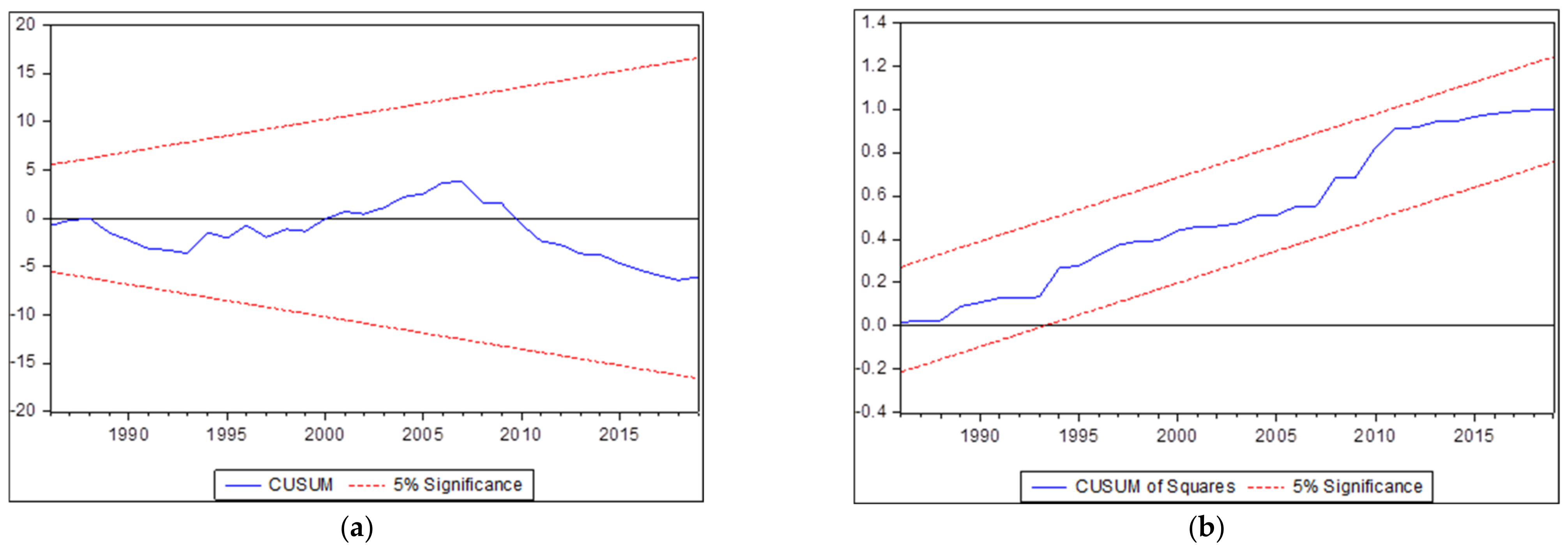
The structural stability of the VECM model was tested using CUSUM tests, which were performed with a 5% significance level. The null hypothesis is that “there are no structural breaks in the system”, with a significance level of 5%. The results show that there are no structural breaks and the presence of stability is fit for IRF. Figure 3a depicts the results of the CUSUM test.

The CUSUM square test indicates the lower and upper bounds of the 5% level of significance for residuals. The results show there is no structural break in the system as residuals are inside the percentage level of significance, making it fit for IRF and forecasting, as shown in Figure 3b.

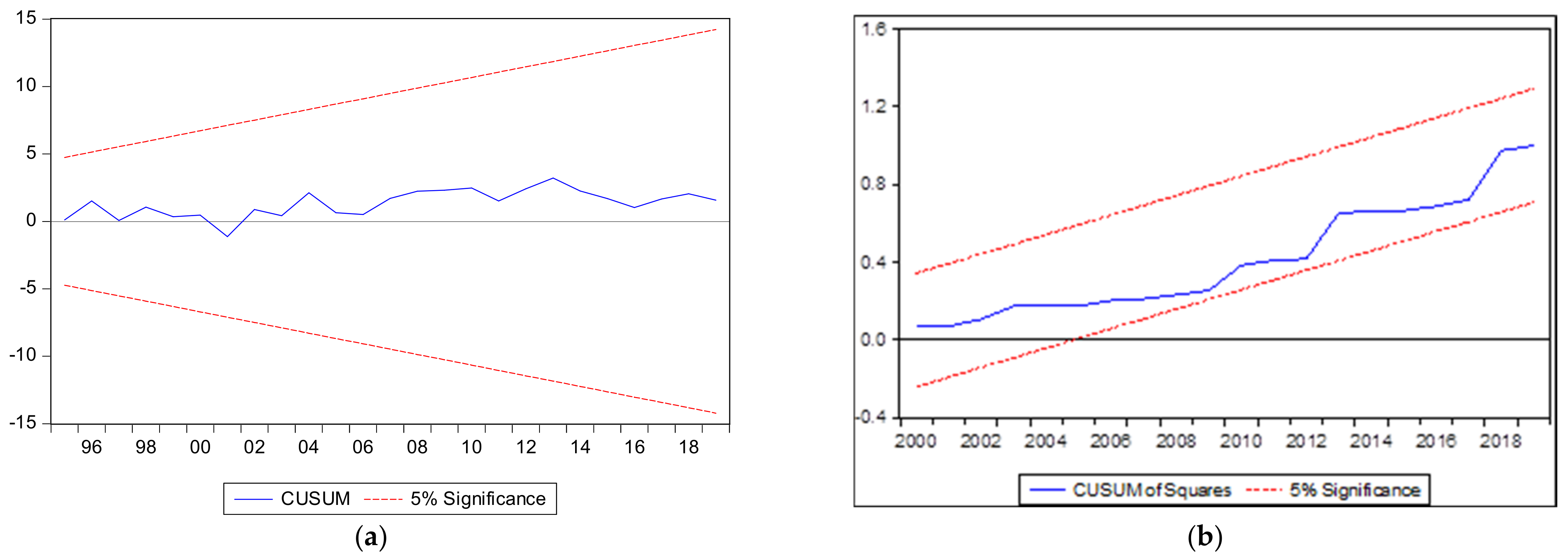
Figure 4a,b The structural integrity of the China series. No structural break exists in the system based on the CUSUM and CUSUM square lines that lie within the 5% significance level.

The structural integrity for the UK series was also tested. The results revealed that the CUSUM and CUSUM square lines lie inside the 5% significance level and the series is fit for forecasting, as shown in Figure 5a,b, respectively.

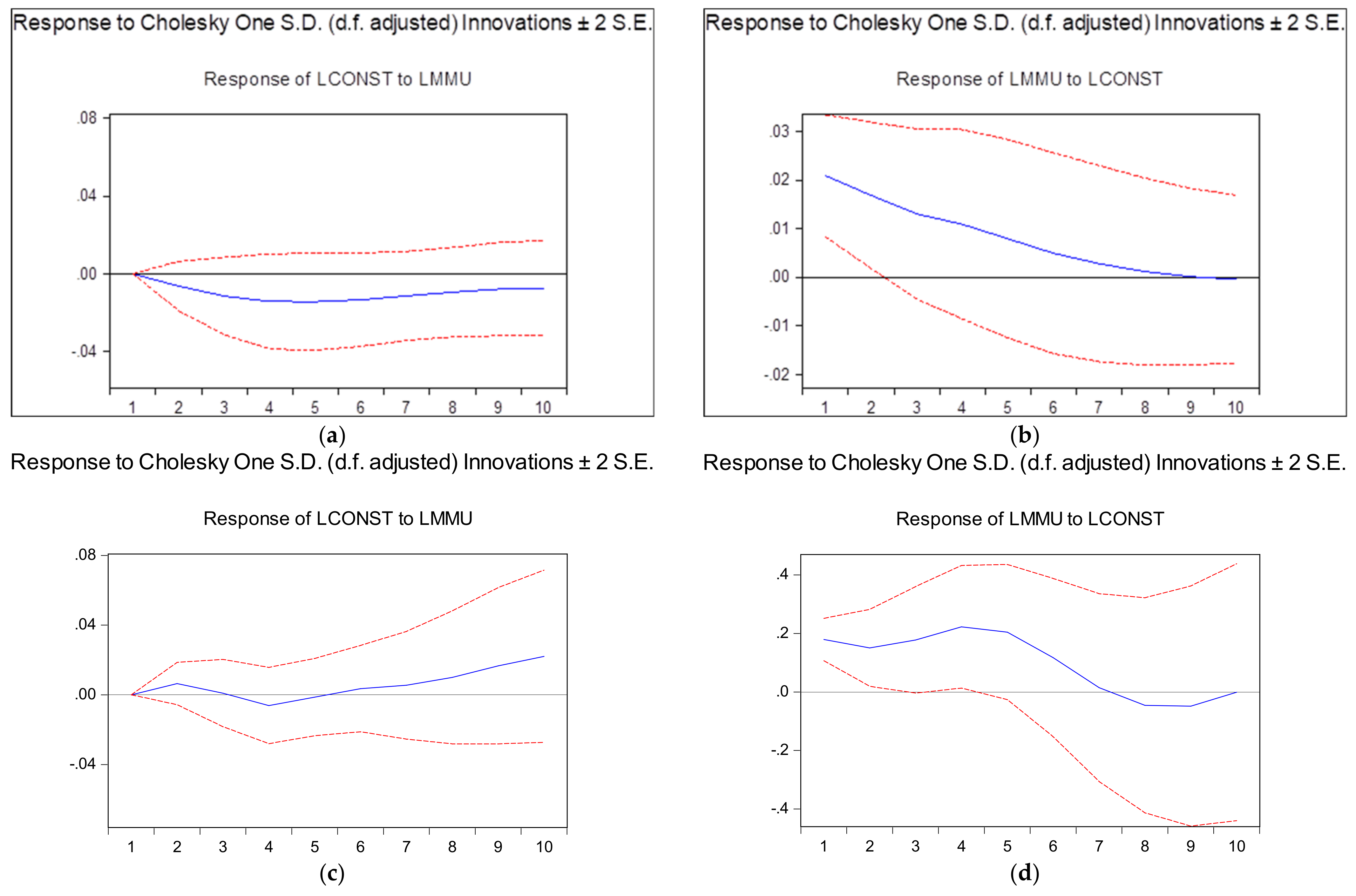
4.8. Shock Responses of the Construction Sector

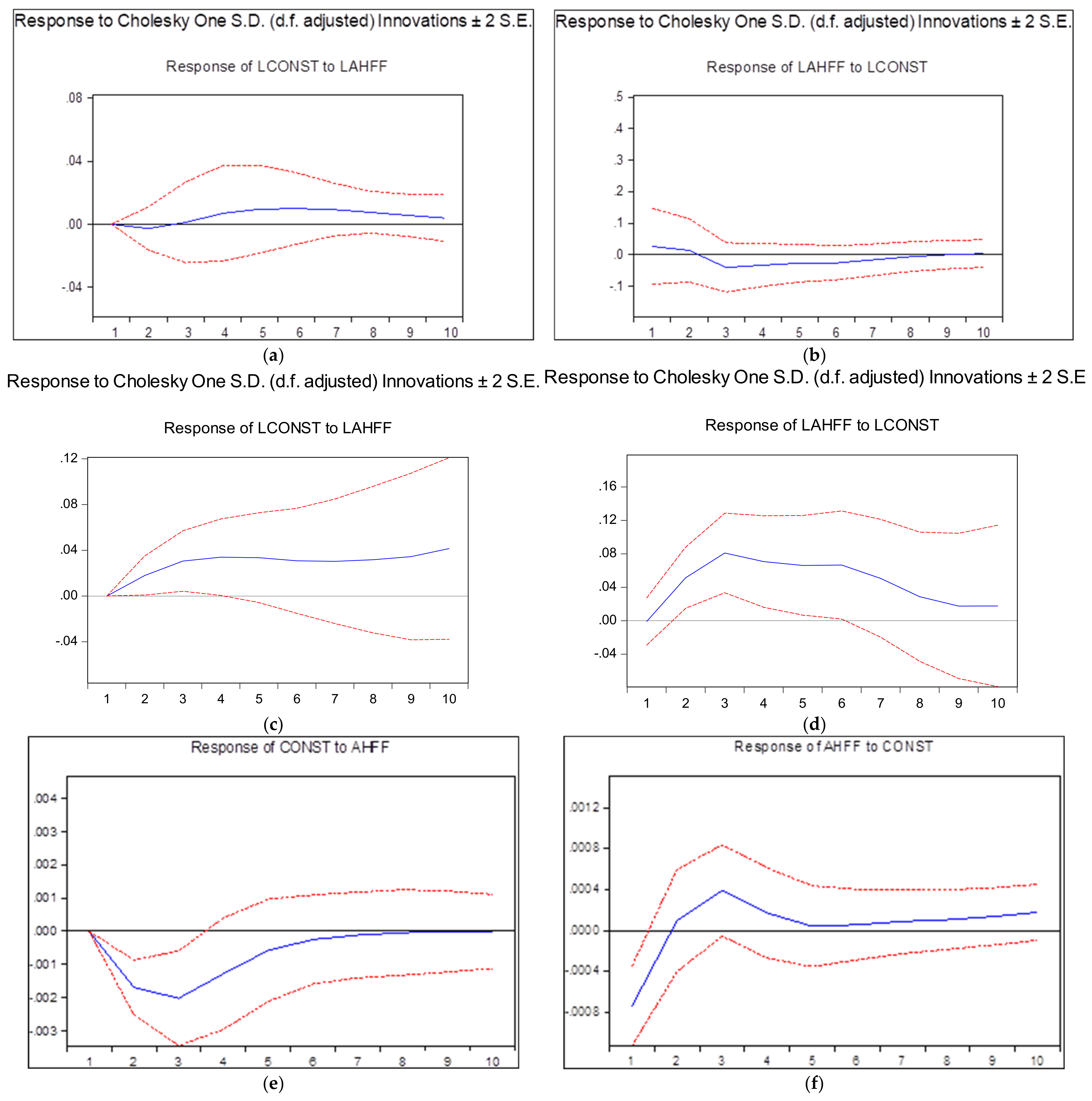
The IRF produces a shock of one time period. In this case, CONST is the endogenous variable. A one-time period shock is given to CONST, and the behavior of other sectors is recorded. The IRF also shows how much time is required for any sector to absorb this shock. In this study, one positive standard deviation shock is produced in CONST, and its behavior is measured in AHFF, MMU, SERV, CONST, and GDP.

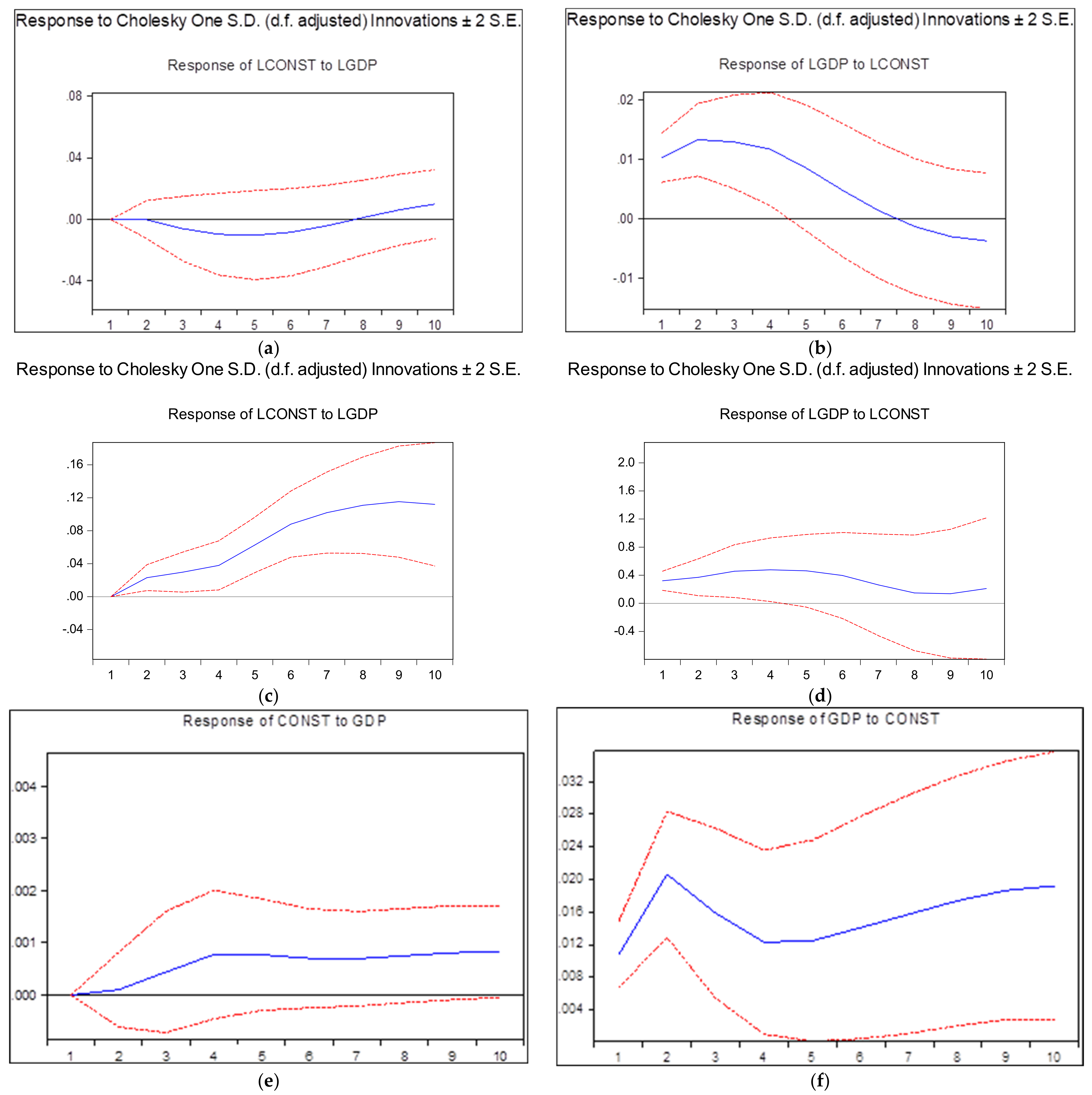
In Figure 6a, the response of CONST is shown after a shock in AHFF in the USA. After the second period (second year), there is a positive trend in the response of CONST. The outcome shows that expansion in AHFF will negatively affect the output of CONST owing to the presence of backward linkages. It will take almost 10 years for the CONST industry to regain its original position from before the shock. Figure 6b reveals that it will take 10 years for the AHFF sector in the USA to recover from a shock produced by the CONST sector. As the linkage is unidirectional, there is no forward linkage between AHFF and CONST; therefore, CONST will not affect the activity of AHFF. Additionally, this sector is not sensitive to activity in the CONST sector.

However, the Chinese construction sector will react differently to the USA construction sector. There will be a positive behavioral shock in AHFF when CONST experiences a shock and vice versa. This result shows that the construction industry of China is more flexible than that of the USA and can drive the construction sector to sustainability. This is shown in Figure 6c,d.

In the case of the UK construction sector, any shock in AHFF will first produce negative effects in the CONST sector and will underperform until the fifth period, and will become stable after the sixth period, as shown in Figure 6e. Meanwhile, the AHFF response will first start with negative effects when the CONST sector experiences any change in its output. After that, there will be a positive effect in the AHFF sector for at least 10 years, which can be seen in Figure 6f.

Figure 7a shows the behavior of CONST when a shock is experienced by MMU in the USA. There is no significant positive trend in the behavior of CONST, and it does not deviate from zero lines, indicating that CONST is less likely to be affected by any change in the MMU sector. The CONST will have less effect on MMU and will not deviate much from the zero lines. Figure 7b indicates the response of MMU when a shock is produced in CONST in the USA. There will be a positive effect on MMU and it will return to its original state without much difference. There will be a significant shoot-up in the MMU sector, which will decrease with time and return to its original position due to the shock in CONST.

Figure 7c indicates the behavior of CONST after any shock is experienced by the MMU sector in China. As evidence, the response of the CONST sector will be stable for the next five years, and then the subsequent five years will show a positive output in CONST. Figure 7d shows the behavior of MMU toward the shock in the CONST sector, where there will be a positive change in the production and activities of MMU, which will stabilize as the period approaches its 10th year.

Figure 7e shows that the first two periods will negatively impact the CONST sector when the MMU sector receives a shock. However, this change will dissipate with time and there will be no major effects on the CONST sector in the UK. Figure 7f illustrates the positive response in MMU when the CONST sector receives a shock; there will be an increase in production for at least 10 years in the UK.

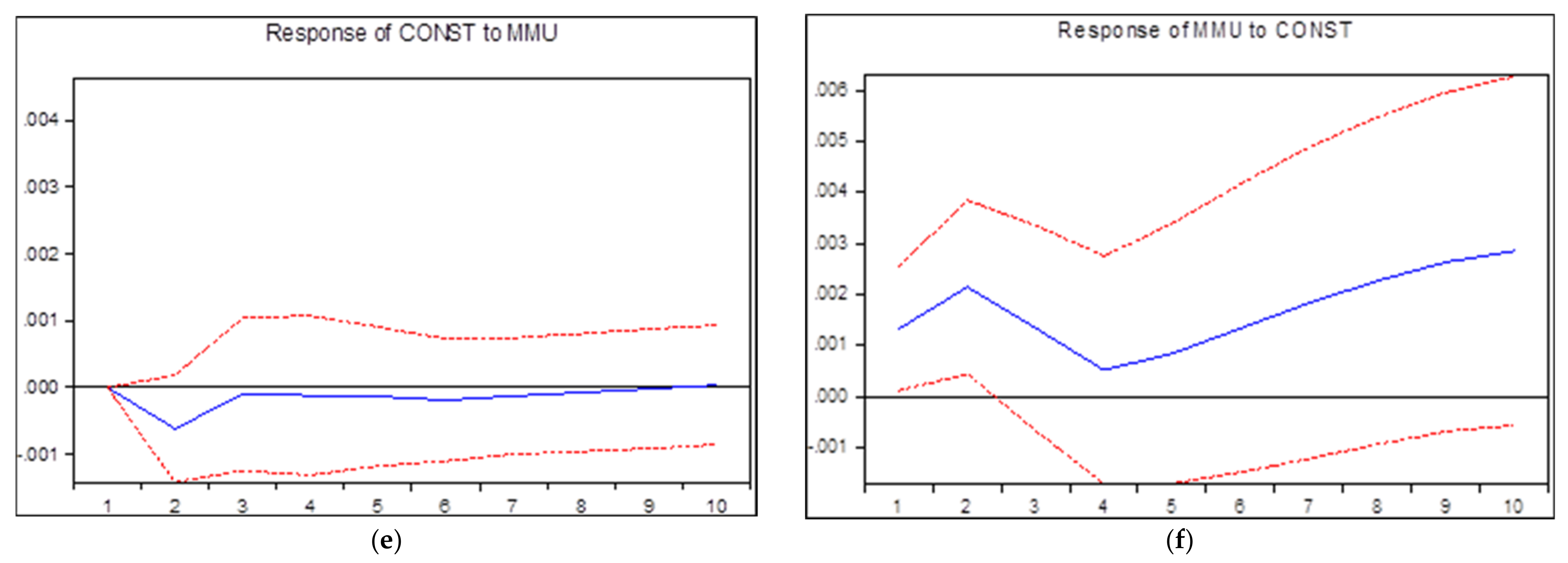
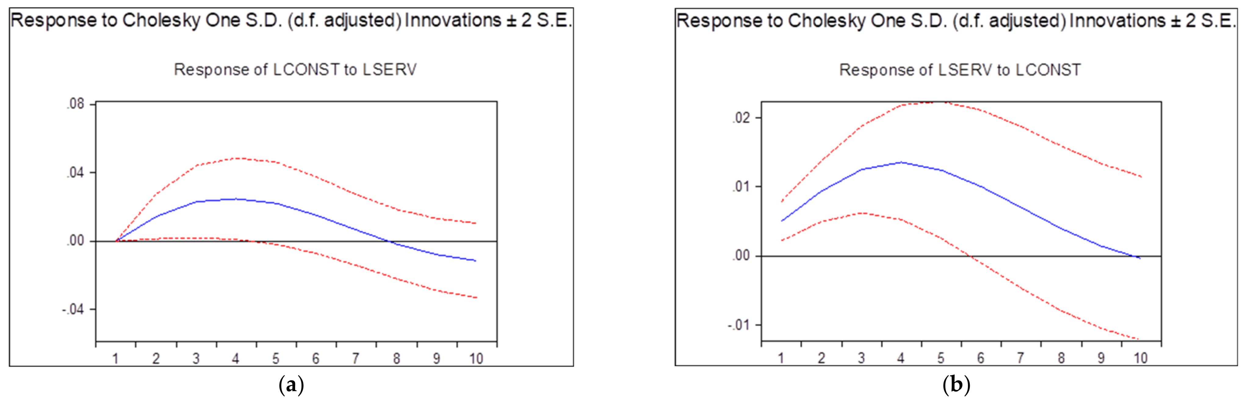
Figure 8a shows the behavior of CONST after a shock is produced in the SERV sector in the USA. There will be a positive trend in CONST when SERV experiences a shock of one time period. As SERV-CONST has a forward linkage, any positive shock will result in a positive output. The shock will stabilize after the eighth period. Figure 8b reveals that the shock produced in SERV will positively affect CONST, which will decrease with time due to the stored services used in the construction industry, such as petrol, transportation, and material supply.

Figure 8c signifies the positive behavior in the CONST sector in China when there is a unit shock in the SERV sector during the first five years. After that, the CONST sector will lose its productivity because it is greatly dependent on services for the timely execution of projects. Figure 8d shows the positive behavior in the SERV sector when there is a lack of funding or recession in the CONST sector, positively affecting the performance of the SERV sector.

Figure 8e shows that the UK SERV sector will produce marginal positive effects in the CONST sector until the fifth period, after which it will decrease as it approaches the tenth period, and will stabilize after this period. Figure 8f indicates the positive behavior in the SERV sector of the UK after the CONST sector experiences a shock. The positive effect will continue beyond the tenth period.

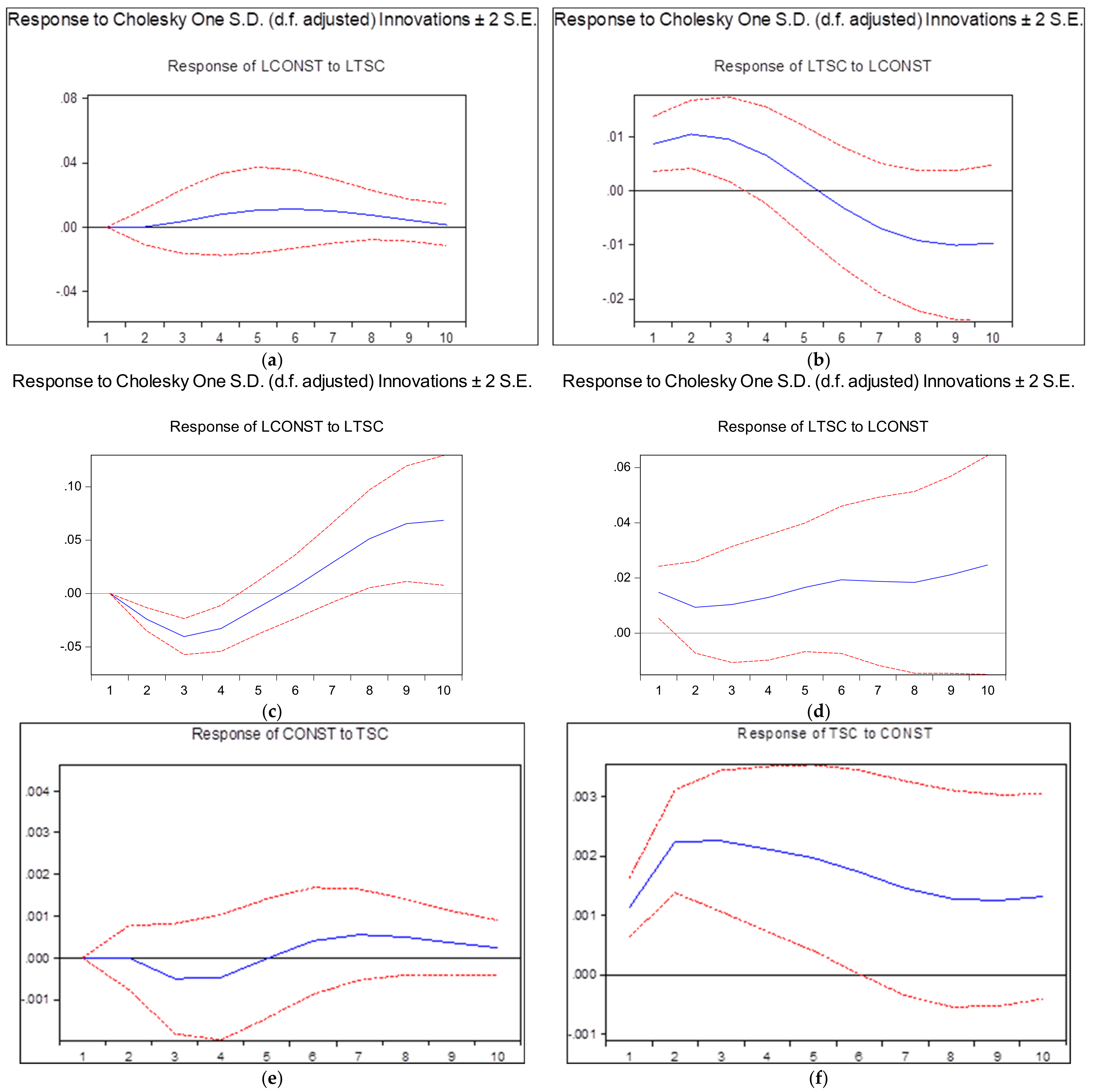
Figure 9a illustrates that no significant changes will occur in the CONST sector when a shock is received in the TSC sector of the USA. There will be a slight positive trend, but this trend will not affect productivity and production in the CONST sector. This behavior validates the findings of the Granger causality, in which there is no linkage of CONST-TSC. Figure 9b shows the behavior of the TSC sector to a shock in the CONST sector, which will positively affect the performance of the TSC sector until the first half of the fifth period (year). After that, there will be a negative effect on the TSC sector due to the shortage of transportation of materials and vehicles, expensive storage, and expensive communication.

Figure 9c shows the negative behavior of the CONST sector toward the end of the fifth period after a shock is received in the TSC of the Chinese economy. However, a recovery will be made in the sixth period and positive effects will start to manifest themselves. Figure 9d shows a positive response for 10 consecutive time periods in the TSC sector when a shock is received in the CONST sector of China.

Figure 9e indicates the negative and positive behavior of the CONST sector after the TSC sector of the UK receives a shock. The negative effects in the CONST sector will continue for five time periods and, after that, there will be a positive output in the CONST sector owing to any change in the TSC sector. Figure 9f reveals that a shock in the CONST industry will positively impact the growth of the TSC and the sector will grow efficiently.

Figure 10a shows the non-significance of CONST-GDP in the USA. As there were no Granger cause linkages, there is only a minimum effect on the performance of CONST by any changes in the GDP. The shock in the GDP of the country will move to negative, which returns to its original position in the eighth year. A positive trend will also be shown toward the end of the tenth year. Figure 10b indicates the Granger causes’ forward linkage direction effects. Any shock to the CONST industry will greatly affect the performance of GDP.

Similarly, the Chinese CONST sector will grow considerably after the overall GDP is affected due to any shock. This effect will be longer because the CONST sector of China is the largest in the country, and China will invest all the capital in CONST to boost its overall economy, as shown in Figure 10c. Figure 10d shows the positive change in GDP after a shock is experienced by the CONST sector, although it will be short-lived, and will stabilize as it approaches the end of the tenth period.

Figure 10e shows the positive impact of the CONST sector after the overall GDP of the UK is affected by any shock. There will be a slight increase in the output of the CONST sector, which will continue beyond 10 time periods. Figure 10f illustrates that any shock in the CONST sector will positively affect the performance of the GDP of the UK. Like China, the UK will also support the CONST sector in the case of any shock, which will increase the overall performance of the UK’s GDP.

4.9. VECM Forecasting

The forecasting was performed for the USA, China, and UK construction sectors from 2021 to 2050. Based on the findings, the construction sector of the USA is predicted to grow more than twice as much in 2050 as it did in 2020.

Similarly, with China and the USA being at the same point in construction output in 2019, this gap will grow significantly over three decades. The contribution of China’s construction sector to the national GDP will increase a little over USD 2 trillion in 2050. However, there will be no significant change in construction output in the UK in 2050. This forecast was made by considering no effects to the laws, policies, and unseen events such as COVID-19. The forecasted values will change significantly if there are pandemics in the future, which will seriously affect the national and global trade-off. The forecasting estimation is shown in Figure 11.

5. Conceptual Framework

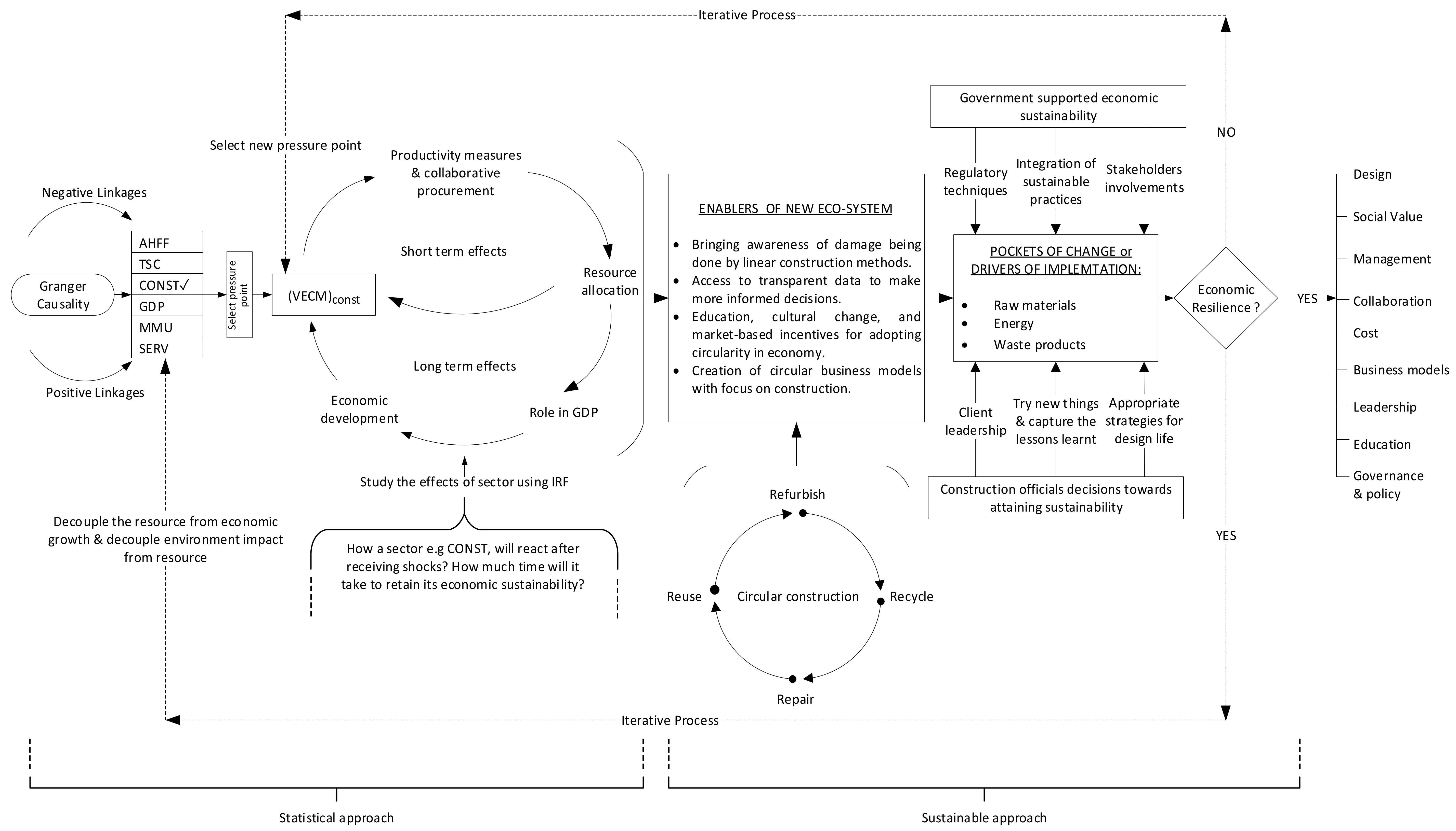
By studying the effects on these countries, a sustainable framework was suggested, as shown in Figure 12 that could combine the effects on these countries and be applied on a large scale following the practices of sustainability and economic development in the CONST sector. First, the directions of linkages among the various sectors are identified [85]. As this study focuses on the CONST sector, this sector is taken as a reference. After the linkages are identified using the Granger test, a pressure point is selected in the CONST sector (e.g., plastic). The short- and long-term effects of the pressure point (such as plastic) are evaluated using VECM. The effects of pressure points are taken into account and their behavior is assessed using IRF when a shock is experienced due to the change in pressure point in the sector. This step constitutes the statistical approach of the framework. The statistical approach and sustainability approach of the construction sector are linked through the enablers of a new ecosystem. The novel economical ecosystem can be created by the conglomeration of circular construction techniques that are financially viable for the pressure points. This includes determining the short- and long-term effects of the pressure points through industrial ecology, eco-economical techniques, outreach and collaboration of new business models, and the eco-designs of the pressure points. Hence, the combined support of government officials and construction bodies can make the necessary shift required for the implementation of sustainability in the economy and the processes of the pressure points. This shift can be regarded as a pocket of change, which can be seen in recyclable materials, optimization of energy efficiency, and circular use of waste materials from construction activities [86]. This will result in the economic resilience of the pressure points, which will directly produce resilience in the design, cost, business models, processes leadership, and government policies of the sector.

The statistical results obtained from this study could be merged with the sustainable procedures. One similar study showing the sustainability outcomes using time series analysis by calculating the carbon footprints was performed. It was found that the time series analysis could provide solutions for sustainable product designs, and sustainable procurement of raw materials [87]. The novelty of this study is that it shows how statistical results could be used to pave a way for sustainability. The use of Granger causality to assess the direction, and the usage of VECM to determine the long- and short-term effects of the behavior of the sector make this framework applicable. The results obtained from the statistical portion would show the fluctuation in the sector after receiving a shock, which could be studied; thus, sustainability concepts could be applied to counter the shocks in the sector. Moreover, the sustainability part of the framework is mostly theoretical, which could be applied to drive the sector towards sustainability.

Comparison of the construction sectors of three developed countries was performed to assess the behavior of the construction sector towards a shock. By setting a standard of behavior for these countries, other countries could benefit by observing how much their respective countries could sustain a shock and how the aftershocks would affect the national GDP; in this way, a great deal of economic recession could be prevented. The comparison was also performed to study the effects of the construction sector of each country on the IRF with subsequent proposal of a global circular framework with suitable application globally.

The value changes over time also entail environmental development. For example, the use of asbestos in construction was once lauded for its fireproofing properties but is now considered dangerous to environmental and social sustainability, as is the case with conventional construction procedures. Hence, the concept of cleaner production, such as social sustainability, environmental impact, and the built environment, is a continuous process. The application of circular strategy implications intensifies the use of “a balance of minimizing the carbon production with economic energy methods” and enables the intensification of redesigning, reusing, and recycling resources. Selective strategies for repairing and maintaining should likewise be applied to ensure efficient upgrading in the construction sector. Finally, the combination of recycling and reusing renewable materials must be made a part of circular strategies to achieve cleaner construction practices.

6. Discussion

The quantitative analysis of this statistical analysis revealed the contribution, output per period, and average growth of all sectors in relation to the overall GDP of the USA. The average contribution of the CONST sector to the AHFF sector is the smallest with regard to the overall GDP, compared to other sectors of the USA. Similarly, the CONST and AHFF sectors of the UK had a correlation of 85.7%, which were the least correlated, similar to the USA. All the sectors of the USA and UK had first-order integration while China’s order of integration was two, suggesting the long-term effects on the variables in these countries. The VECM was selected for modeling long-term relationships. A VECM system indicated the presence of an error correction system in the variables. The long-run coefficient C(1) shows an ability to bounce back to equilibrium. The first coefficient C(1) in the system of variables indicates the speed of adjustment toward the long-run equilibrium of the CONST industry as 0.267%. The negative value of coefficient C(1) implies a negative long-run association with the CONST industry while SERV has a positive association with the CONST sector. This finding means a positive growth or expansion in AHFF, MMU, and TSC will have negative impacts on the growth of the CONST sector. The coefficient C(2) is the short-term speed of adjustment, which means that a percent increase in AHFF will result in a decline of 0.09%. Similarly, a percent increase in C(3) (MMU) will result in a decrease of 0.8% in the CONST sector.

The analysis period selected in this study was from 1970 to 2021. After COVID-19 was declared a pandemic by the World Health Organization (WHO) in 2020, most countries adopted lockdowns nationwide as a preventive measure, which negatively impacted the performance of all sectors. The inclusion of COVID-19-impacted data in this analysis would have produced different results, but it was not made a part of this study due to the unavailability of the officially released data for 2022. It was likewise impossible to analyze the hidden factors that are constantly changing, which would lead to uncertainty in the results. This study performed statistical analysis on the construction sector and other sectors associated with it, and identified the obstacles that should be addressed to make the sectors self-sufficient. It also identified the challenges that are hurdles in achieving sustainability in the construction sector. Any percent change in the construction sector will affect the overall output of the country, depending on how each country takes effective measures to prevent the sector from slipping into recession. The analysis of the construction sector of three countries shows that a sector without any sustainable vision will produce satisfying growth in the short term. However, in the long term, if the rapid implementation of legislation for reducing hydrocarbon emissions is needed, it will prove detrimental to the sector.

6.1. USA Economy

It is expected that the construction industry environment in the USA will become favorable in terms of decreased tariffs under Joe Biden’s presidency, given that Trump had increased the cost of construction during his administration, though he did announce a USD 2 trillion relief package for infrastructure development [88]. Accordingly, the USA pledges to cut the use of hydrocarbon fuel and its emissions up to 52% by 2030 [89]. The residential construction sector plays an influential role in the development of construction. Owing to the shock in the economy from the COVID-19 outbreak, millions of people were laid off from construction, which forced first-time buyers to look for low-cost, large spaces for living [90]. However, a question remains about the uncertainty of expansion of residential construction because of COVID-19 lockdowns, which have paralyzed business in this field. It is estimated that the global construction output will increase to USD 8 trillion by 2030, and the top three contributors to construction will include the USA and China, which have a combined construction output of 57% of global growth [91]. Construction in the southern states of the USA is expected to increase, reflecting the higher population growth and catch-up potential of the region. In the next 15 years (up to 2035) [92], the construction industry of the USA will grow faster than in China and will become more dynamic, which will influence the evolution of the prosperity of the society as it will create a vast number of jobs and will ensure wealth and a healthy living standard of the people [93]. Hence, output growth in the construction sector will increase the overall GDP and bring socio-economic prosperity to the country.

6.2. Chinese Economy

Similarly, it is anticipated that the Chinese construction sector will rise to become the largest construction market in the world and will generate USD 13 trillion in revenue by 2030. On the flip side of this marvel development in the construction sector, there will be a draconian production of 28% of the global energy emissions in the absence of sustainable processes [94]. The five-year plan for the sustainability of China limits the use of fossil fuels to 20% with each subsequent passing year [95]. China plans to rely on renewable sources for its energy demands, on-site renewable zero carbon emission energy practices and making public and private real estate sustainable, all of which will drive the country toward a 70% reduction in carbon emission by 2060 [96]. China plans to achieve cleaner production in the construction sector through sustainable urbanization and human settlement, reducing the use of fossil fuels, managing household wastes for rural and urban areas, formulating urban air quality standards, constructing ecological corridors, restoring wetlands, and improving energy savings for existing buildings [97]. To embark on the cleaner environment strategy, as the primary carbon polluters of the world, China and the USA have agreed to cooperate to tackle the climate crisis based on its urgency and reduce fossil fuel emissions by half [98].

6.3. United Kingdom Economy

It is expected that the UK construction sector will surpass the German sector and become the sixth-largest construction sector and the largest one in Europe by 2030 [99]. The UK has introduced the vision Construction 2025, which includes benefits such as reducing GHG emissions by 50%, reducing construction costs by 33%, building cheaper homes and ensuring their fast delivery by 50%, designing smart and safer buildings, sustainable practices, and cleaner production [22]. The World Economic Forum introduced the Infrastructure and Urban Development Industry Vision 2050, which envisions minimum carbon and resilient construction solutions. The application of low-carbon emissions and innovation of cleaner practices can be implemented through the collaboration of the stakeholders, performance-based delivery of construction practices, a skilled workforce, use of digital systems to optimize social, economic, and social benefits, reducing risks by responding quickly to the losses, and application of a long-term lifecycle of optimized solutions [100].

The VECM analysis of Australian construction markets shows that other sectors’ price hikes increase construction prices, which is also evident in this study, with other sectors such as SERV, TSC, MMU, and AHFF increasing in price [101]. In another study to forecast construction demand in Australia, it was found that the VECM model of forecasting construction demand was affected by GDP, population, and exports [102]. The results of this study also indicate that the construction sector has forward linkages to GDP and other sectors. An empirical investigation of the construction sector and economic growth was performed in Saudi Arabia. It was found that there is a unidirectional causality and long-run effects in the construction sector [103]. This study also revealed that there would be short-run effects of a shock in the construction sector and long-run effects on other sectors’ behavior along with economic growth.

Although many studies were conducted to study the behavior of the construction sector and its contribution to the cumulative economy, there is an absence of studies that use statistical processes such as IRF to study the behavior of the construction sector toward the road to sustainability and cleaner production. Therefore, this study closes the literature gap by proposing the use of statistical inferences that can be employed in a circular economy to bring the construction sector one step closer to sustainability.

The methodology followed by the current study suggests that IRF can adequately be used to forecast shock behavior by creating an impulse in the multivariate vector autoregressive function. This statement validates the methodology followed by previous studies, indicating that a single variable can have instantaneous effects on the second to last variables; therefore, the concept of the shock is the correct representation within the economic system.

How, then, can the construction sector be made a sustainable sector? First, we have to invest in work density, which is the only way to be energy-productive, resource-productive, flow optimally, and use the stock of resources optimally. Second, we have to make sure it is diverse in a way that can be used within the work density. Third, work density must be reintegrated back into the city. Finally, the novel availability of renewable resources and the accessibility of micro-mobility must be returned to construction sites.

7. Conclusions

This study used a dynamic statistical approach to determine the role of each sector in the cumulative economy. Three countries (the USA, China, and the UK) were selected as the scope of analysis to study the behavior of the CONST sector. Based on the results, it was concluded that the CONST sector is volatile, can trigger a recession in the economy, and behaves differently to other sectors due to its nature. The CONST sector has short- and long-term effects on itself and other sectors. To achieve sustainability, the CONST sector would have to make use of carbon processes to return to its original position after experiencing a shock. After regaining its former position, only then could the CONST sector move towards sustainability; hence, for this purpose, a combination of statistical processes and the pillars of sustainability must be followed. Adopting new pressure points and analyzing their effects in the sector, along with their quantitative role in the CONST sector, could lead to sustainability in the sector. However, the absence of a sustainable framework to support these sectors will lead to environmental degradation, which can be prevented by implementing the proposed framework.

The USA is facing challenges in the CONST sector due to the hike in prices of major materials for construction and lack of employment. Aside from other reasons, the COVID-19 pandemic has also disrupted the overall sector. Currently, the hurdle in the UK construction sector is to enable the local skilled workforce to adopt digital mechanistic approaches while retaining the current labor force and its traditional knowledge of construction techniques. This scenario leads to poor productivity and insufficient innovation, which draw attention to and emphasize sustainable novel procedures in designing and planning. The challenges faced by the Chinese construction sector include environmental problems, such as excessive pollution, the difference in income between Eastern and Western construction workforces, insufficient capital funding, and strict banking loans for supporting the construction sector.

The theoretical framework selected for this study best suited and was proved adequate to answer the research problems. The use of Granger and impulse response concepts established that the construction sector is linked to other sectors, with dynamic output effects on future series; hence, the variable satisfies the hypothesis of linkages and the effects of the study of economic sectors.

In light of the above conclusion, the following research hypotheses were concluded. Firstly, the CONST sector is greatly dependent on other sectors for its material supply; any major change in this sector would also affect the performance of other sectors; hence, the related hypothesis is rejected. Also, recovering from a major shock would require an increased demand in energy, which would increase the threshold to attain sustainability in the CONST sector. Secondly, the construction sector must move beyond sustainable processes to achieve its former position and construction should move in the same direction as the national economy to regain its former GDP growth. Thirdly, investors and policy makers should pay attention to emphasizing a cleaner construction sector in terms of policies, stakeholder trust, human resources, and capacity-building programs; hence, the related hypothesis is rejected. Finally, the results of the IRF and VECM could be incorporated to assess the behavior of the construction sector if sustainability is introduced in this sector; hence, the related hypothesis is rejected. Hence, the short- and long-term effects of the construction sector on employment, output, and circularity indicate that to regain its original position, the construction sector would have to make excessive use of CO₂ to run its engine; therefore, in the long term, the construction sector would become unsustainable.

8. Recommendation and Future Prospects

This study recommends an in-depth examination into the identification of problems facing the construction sector, which has the potential to generate a considerable output and prove fruitful in helping the country recover from times of economic recession. Joint venture programs between multinational firms and local authorities must be increased to grow human capital, increase skilled labor for cleaner production, execute required work in decreased time, achieve resource efficiency, and develop machine-operating skilled workers. Knowledge sharing should be encouraged to increase the trust of local and overseas investors, which will raise foreign direct investments in the construction sector that could pave the way for a circular strategy. Finally, the process of tendering, sustainable construction methods, integrated solutions for the development of methods, loans and funding for research, contract agreement, and transparent payment procedures must be applied to the construction sector, which will attract many stakeholders to invest in innovative procedures in the sector.

Future research should focus on construction multipliers. This study used the GDP of the CONST sector but data were limited. In the future, other contributing factors, such as health, revenues, employment rates, biodiversity loss, and material consumption, must be analyzed to reflect the accomplishment of suitable practices in the CONST sector. This will help determine the factors for lagging in sustainable development, hence enabling the government and private firms to make informed policies for sustainable development in the CONST sector. Future work should focus on replicating the statistical procedure in individual geological regions (states or neighboring countries). This individual focus will not only help identify differences at the small scale in the drivers of change and their enablers, but also develop deeper insight into understanding corporate and stakeholder roles.