1. Introduction
Air quality in cities, in particular in relation to PM2.5, is an important topic indeed. It is well known that poor air quality is associated with impacts on human health, both in the short- and long-term [
1]. Recent epidemiological evidence [
2] motivates the need for accounting for fine particles in the scope of air quality regulations. While in the literature the topic of long-term exposure to air quality is well discussed (focusing on action plans to improve air quality in a time-frame of a few years), the issue of short-term exposure is more uncertain [
3]), e.g., it is known that short-term action plans, triggered in cases of forecasted high pollution episodes, are not always effective [
4]. In some cases (e.g., when limiting road traffic, or closing for few days an area to vehicles), only a limited impact on air quality concentrations is observed (in particular in terms of PM2.5 concentrations), and more research in this field is needed [
5]. The difficulty arises from the fact that PM2.5 is produced through complex chemical reactions and dispersion/transport mechanisms, and from various sources, making it challenging to identify how to act to reduce concentration levels [
6,
7]. Modelling methodologies are often used to study the potential of local actions to reduce high pollution episodes in cities.
Usually, short-term action plans and the analysis of their effectiveness are based on model forecasts [
8,
9,
10,
11,
12], differencing model simulations performed with and without a specific set of emission reduction measures. Even if is useful to predict the impact of a plan for a given episode, this information remains specific and does not provide insight on the impact of local strategies on air quality in general [
13,
14].
In this paper, we address the issue from another perspective. We use yearly modelling simulations, in which different sources are progressively switched off, to understand their cumulative impact on daily pollution concentrations. We then rank these impacts in terms of low and high concentration days, to see how policies would be effective in tackling different pollution ranges.
The sources considered for this analysis are the cities themselves; the urban areas in the neighborhood (to explore the benefit of coordinated urban actions); agriculture and the remaining anthropogenic and biogenic emissions, to quantify the added value of EU-wide policies.
In comparison to previous papers on this subject [
15], the main difference lies in the use of daily PM2.5 values (not yearly averaged). In addition, in comparison to other similar analyses and visualization approaches (i.e., in CAMS annual source-receptor information, at policy.atmopshere.copernicus.eu), we provide here a combined view on sectors and geographical areas, with a method that is flexible to accommodate any possible geographical or sectoral category.
The model simulations are based on a full 100% switch-off of the sources of interest (city, agriculture…). While this choice allows assessing without any assumption of the full responsibility of the sources, it is not connected to real-life emission reductions that never reach this level. An important question is therefore to address whether we can interpolate these extreme (100% reduction) simulations to lower emission reduction intensities that are representative of local actions. We check this point by assessing the degree of nonlinearities of the model responses in the final part of this work. We also briefly assess the efficiency of local and large-scale actions with respect to other pollutants, such as NO2 and O3.
The proposed methodology is applied to 10 large European cities, to address the following questions:
How much do the city, the surrounding urban areas, agriculture and the remaining EU emissions contribute to urban pollution?
How do these contributions change across city?
How do these contributions depend on specific days (characterised by low or high concentration values)?
The paper is structured as follows: in
Section 2 we detail the methodology; in
Section 3, the results (and the evaluation of the nonlinearities); and in
Section 4 there is a discussion and conclusions.
2. Methodology
2.1. Modelling Set-Up
This work is based on a set of model simulations performed with the EMEP air quality model version 4.34 [
16] for the entire year 2015, fed by the CAMS v2.2.1 emission inventory [
17]. The emission inventory covers all PM2.5 precursor emissions (NOx, VOC, NH3, PPM, SO2) classifying emissions according to the GNFR (Gridded Nomenclature for Reporting) categories. More details on the emission inventories and sectoral split are provided in [
18]. The modelling domain covers the whole Europe, with a spatial resolution of 0.1 × 0.1 degrees. The domain stretches from −15.05° W to 36.95° E longitude and 30.05° N to 71.45° N latitude with a horizontal resolution of 0.1° × 0.1° and 20 vertical levels, with the first level at about 45 m. The EMEP model uses meteorological data from the European Centre for Medium Range Weather Forecasting (ECMWF-IFS) for the meteorological year 2015. The temporal resolution of the meteorological input data is daily, with a 3 h timestep. The meteorological fields for EMEP are retrieved on a 0.1° × 0.1° longitude latitude coordinate projection. A validation of the modelling application (checked against observations) is provided in [
19].
2.2. Selection of Cities and Simulations
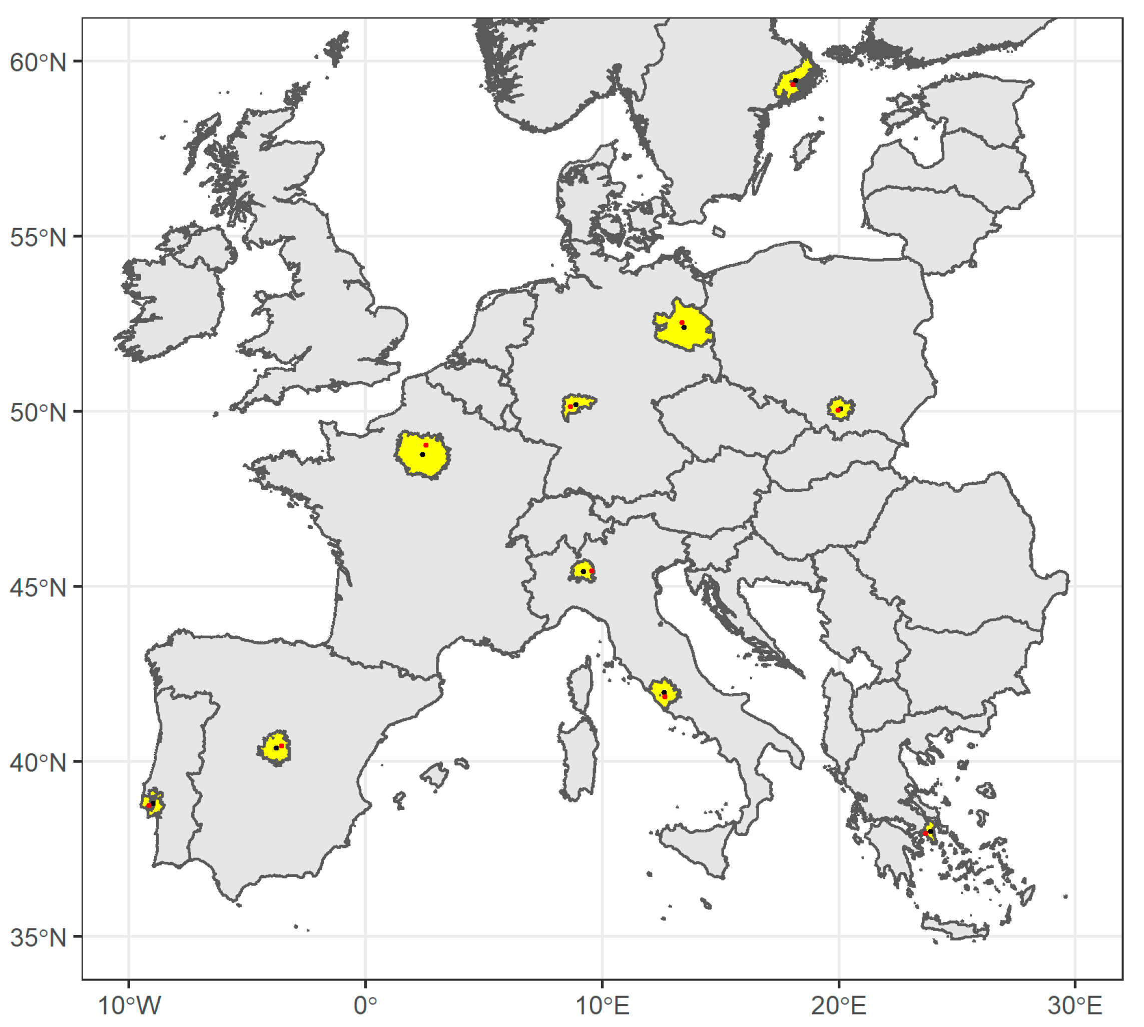
Figure 1 shows the 10 cities considered in this paper: Madrid, Paris, Lisbon, Milan, Rome, Berlin, Athens, Frankfurt, Krakow and Stockholm (for more information on the selected cities feature, please refer to the PM2.5 Urban Atlas, at
https://publications.jrc.ec.europa.eu/repository/handle/JRC126221, accessed on 20 April 2022). These have been selected among large EU cities, to provide a balanced geographical coverage on the EU territory. These cities are defined as a ‘Functional Urban Area’, i.e., composed of a city core and a commuting zone. The city core is the local administrative units, with a population density above 1500/km
2 and a population above 50,000, where the majority of the population lives in an urban centre and the wider commuting zone consists of the surrounding travel-to-work areas where at least 15% of the employed residents work in the city.
The simulations performed on these 10 cities are designed with incremental emission reductions:
The ’baseline’ simulation (reference), considering the 2015 as reference year.
The ’city scenario’: in which all the emissions from the 10 cities are switched off. As cities are far away from each other, we assume that impacts from other cities on the city of interest are negligible.
The ’urban scenario’: in which emissions from all urban areas with a population > 300/km2 are switched off, in addition to the 10 cities themselves. This scenario allows for estimating the additional benefit of reducing urban emissions around each city.
The ’agriculture scenario’: in which agricultural emissions are switched off, on top of the ’city’ and ’urban’ reductions. This is useful to evaluate the additional benefit on urban air quality of reducing one of the main emission sources in rural areas.
The ’EU wide scenario’: in which all-anthropogenic emissions remaining in Europe (here intended as the modelling domain) are switched off. This simulation is intended to assess the additional benefit from EU wide actions (the background contribution is derived by the baseline concentration simulation, summing up the components related to sea salt and dust).
Starting from these runs, the analysis in the following sections is then based on the ‘relative potential’ indicator computed with PM2.5 daily values, as:
where PM2.5
BC and PM2.5
scenario represent the baseline and scenario PM2.5 daily concentrations; and α the emission reduction strength.
For this analysis, all aforementioned scenarios are based on a 100% emission reduction, i.e., a value of α equal to 1. To test the validity of interpolating these extreme emission reduction scenarios to moderate reduction values more representative of local action plans, we performed simulations (on a reduced set of cities) with emissions reduced by 10%, 20% and 50%. It means that, in those cases, the ‘relative potential’ indicator is then used with α values of 0.1, 0.2 and 0.5, respectively.
As mentioned above, we focus our analysis on daily averaged PM2.5 concentrations in 10 cities (see
Figure 1). While the sources have been already defined (city, urban areas, agriculture and EU), we also need to define the receptor, i.e., the location where we quantify the different contributions. Two receptors are selected:
These 2 locations are selected to assess the spatial sensitivity of the contributions. In the final part of the paper, an additional point (the one with the highest value for ‘highestConcentration × population’) is also considered.
3. Results
We structure this section into three parts. In
Section 3.1, we motivate the choice of PM2.5 as the most challenging pollutant in terms of selecting the appropriate time and scale for actions. In
Section 3.2, we analyse the source contributions to PM2.5 daily values and assess how they vary in terms of city and type of episodes. Finally, in
Section 3.3, we assess the robustness of the results, by quantifying the importance of the nonlinear effects. This step serves to estimate the possibility of interpolating our full emission reductions to lower reduction strengths more representative of practical policies. We also discuss the dependency of our results on the temporal dimension.
3.1. Why a Focus on PM2.5
It is important to stress that responses to local and wider-scale emission changes largely differ from one pollutant to the other. Although we focus on PM2.5 in this work, we also briefly address other pollutants, in particular O
3 and NO
2.
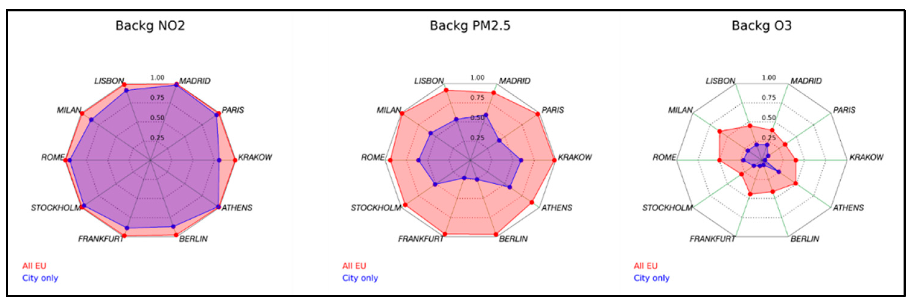
Figure 2 compares the local (red) and EU wide responses (blue) obtained from EMEP simulations, for NO
2, PM2.5 and O
3. To obtain the local responses, emissions have been totally switched off over the functional urban area (FUA) of each of the ten cities. Responses are then expressed as relative fractions of the base case concentrations at the city centre location (see
Section 2). EU responses represent the fraction of the base case concentration reduced when all emissions in Europe are switched off. For NO
2, almost 100% of the concentration can be explained by local emissions. This proportion lowers to 50% or less for PM2.5, and to 25% or less for O
3. While the remaining fraction of PM2.5 can be related to EU wide emissions, this is not the case for O
3, for which about half of the base case concentration is related to background values that do not depend on EU emissions (over the time scale considered, here 1 year). The remaining O
3 levels [
21] depend on other factors such as contributions of methane [
22], hemispheric transport [
23], stratospheric intrusion [
24], etc.
Figure 2 (showing, for different cities and scenarios, the ‘relative potential’ as previously introduced in
Section 2) clearly highlights the need for a pollutant specific strategy, itself varying across cities. More specifically,
Figure 2 shows how policies (at different levels) can improve air quality differently, depending on the pollutant and city considered.
Indeed, while O3 is mostly driven by large-scale processes and NO2 by local processes, PM2.5 shows a mixed behaviour, therefore more challenging to translate in terms of policy. This complex behaviour calls for a focused analysis for this pollutant.
3.2. Contribution to PM2.5
3.2.1. Yearly Average Results
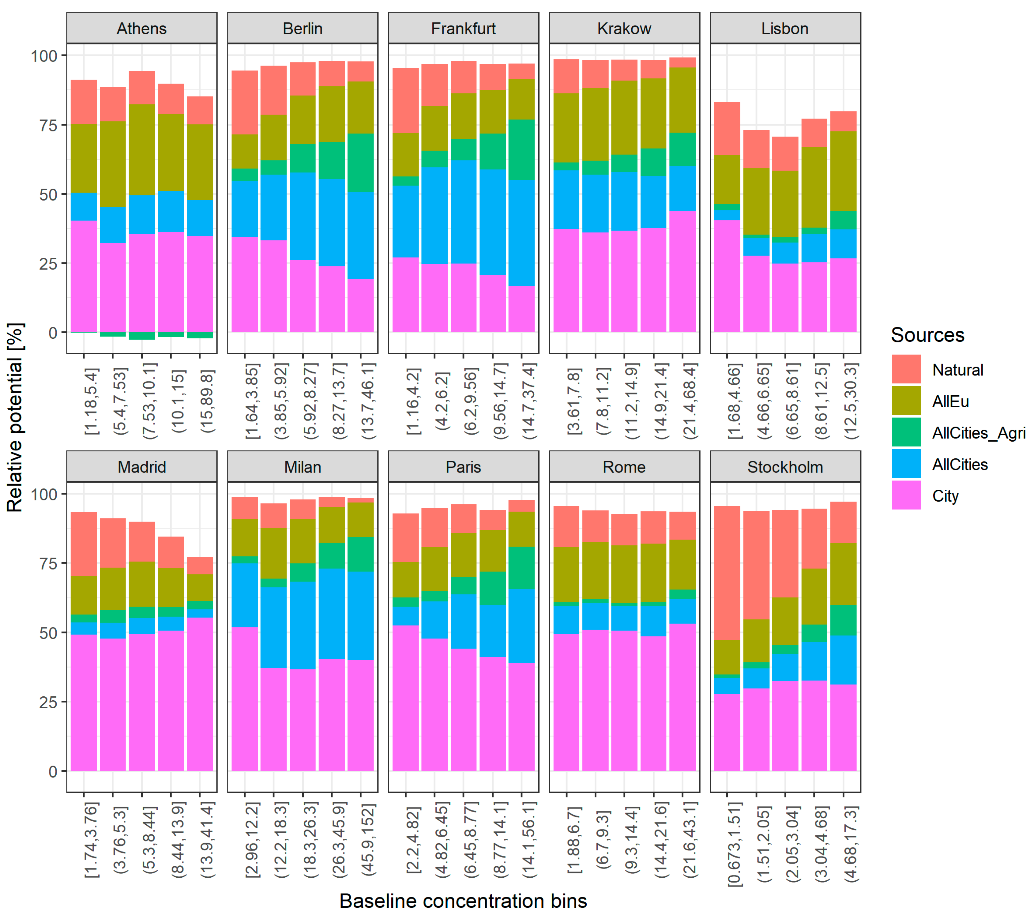
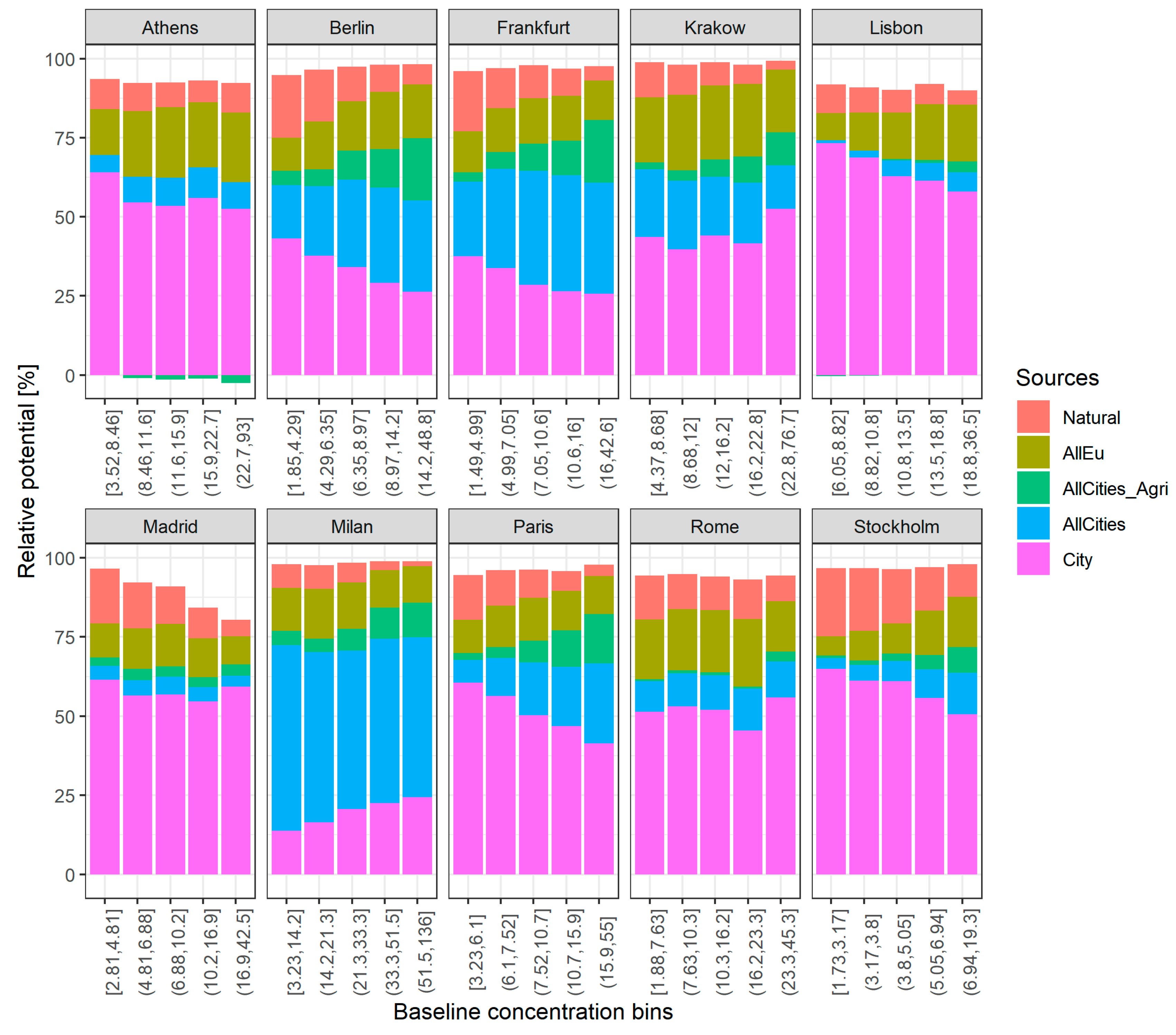
Now focusing on PM2.5,
Figure 3 shows the impacts of different sources (city, urban, agriculture remaining EU and natural) on the daily PM2.5 value for the 10 considered cities, ranked in terms of concentration bins. The receptor location for this analysis is the FUA ‘centroid’.
In more detail, in
Figure 3 (and in the following figures), the ‘labels/colours’ represent:
City: represents the case reducing emissions in the 10 cities;
AllCities: represents the case reducing all urban areas emissions;
AllCities_Agri: represents the case reducing all urban areas emissions and agricultural emissions;
AllEu: represents the case reducing all anthropogenic emissions;
Natural: represent the remaining concentrations.
To better explain these results, let us take, e.g., the case of Milan, in
Figure 3. The x-axis shows the baseline concentrations bins for a given city, with a first bin from 2.96 to 12.2 μg/m
3 and a final bin from 45.9 to 152 μg/m
3. Bins are created by splitting daily PM2.5 values in five equal quantiles for each city. In the case of Milan, 20% of the days have concentrations falling between 2.96 and 12.2 μg/m
3, 20% of the days between 45.9 and 152 μg/m
3, and so on. The y-axis identifies the relative contributions to the concentration. For low concentration values (lower bin), up to 50% of the pollution might be reduced by acting on local emissions (Milan city, violet), and an additional 25% from other urban emissions (in blue), while the remaining contributions depend on additional reductions achieved on agriculture and at the EU level. Finally, a small contribution is ‘natural’. The same analysis holds for each bin and for each city. For the ‘highest concentration bin’ (concentrations between 45.9 and 152 μg/m
3), the picture is a bit different with a lower city contribution (around 40%), while the ‘urban’ and ‘agricultural’ emissions have more importance. For the city of Milan, these findings lead to an important message: for high-level concentrations, it is not sufficient to act at the city level (Milan), and cooperation with other cities is advisable. As cities usually implement short-term action plans in isolation when a pollution episode occurs, this brings attention to the potential added value for integrated short-term action plans, at least for some cities.
Among the 10 cities, we identify three groups in terms of behaviour:
Cities in which the ‘city’ impact gets less important when concentrations increase: Berlin, Frankfurt, Milan, Paris, Lisbon. For these cities, local plans are not sufficient to abate high pollution episodes;
Cities in which the ‘city’ impact is independent of the concentration level: Athens, Rome and Stockholm. Local plans will have the same efficiency regardless of the concentration levels;
Cities in which the ‘city’ impact becomes more important when concentration levels increase: Krakow and Madrid. Local plans are then more effective during high concentration episodes.
This analysis clearly shows that the effectiveness of local actions on pollution episodes is city-dependent.
If we focus on the highest concentration bin, only Madrid and Rome can half their concentrations through local actions. For other cities, actions need to be coordinated with other cities or combined with actions at a larger scale (EU) involving other sectors (e.g., agriculture) to be effective.
In the case of Athens, we also note a small increase (negative values) in PM2.5 concentrations when agricultural emissions are switched off on top of the city’s reductions. This signal is very small, and can be explained by some nonlinearities of the system, that become visible when ’piling up the results’ of the different performed incremental runs.
For some cities (Lisbon, Madrid, Athens), part of the pollution remains uncontrollable despite all considered actions. For these cities, initial and boundary conditions (dust, but also sea salt for Lisbon and Athens) play an important role, mainly when pollution levels are high; this is also possibly due to the fact that these cities are closer to the boundaries of the modelling domain.
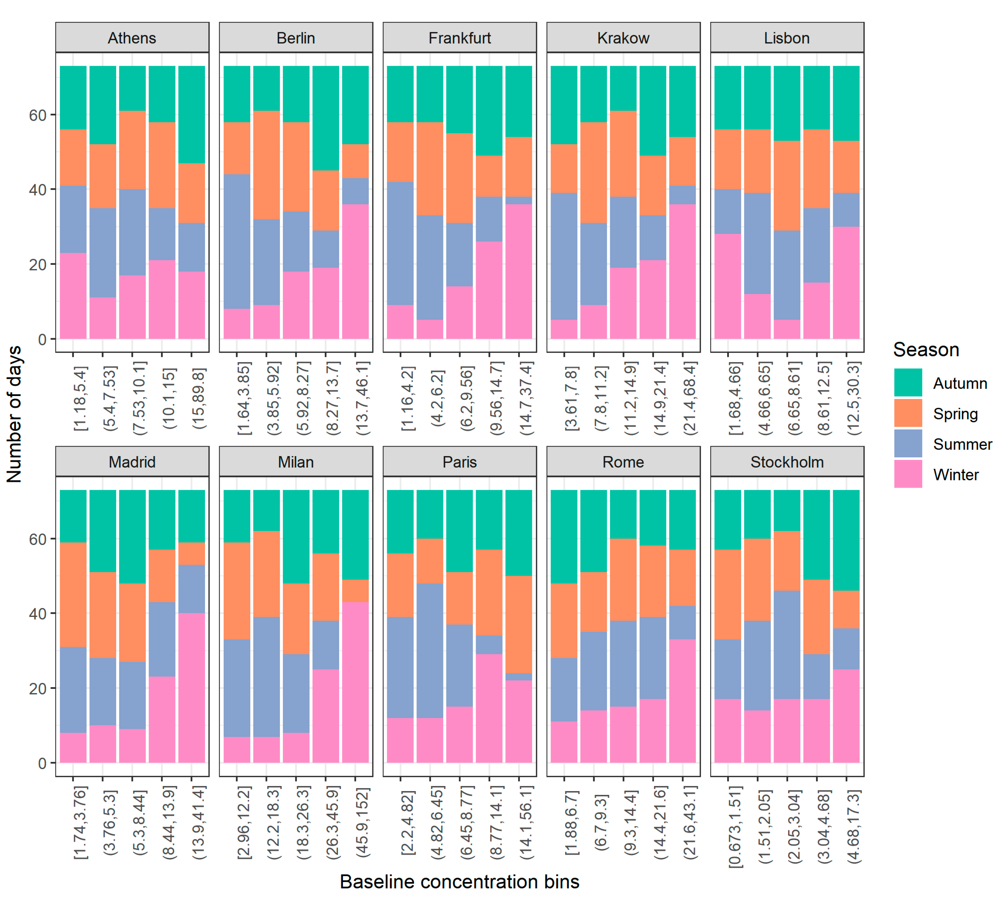
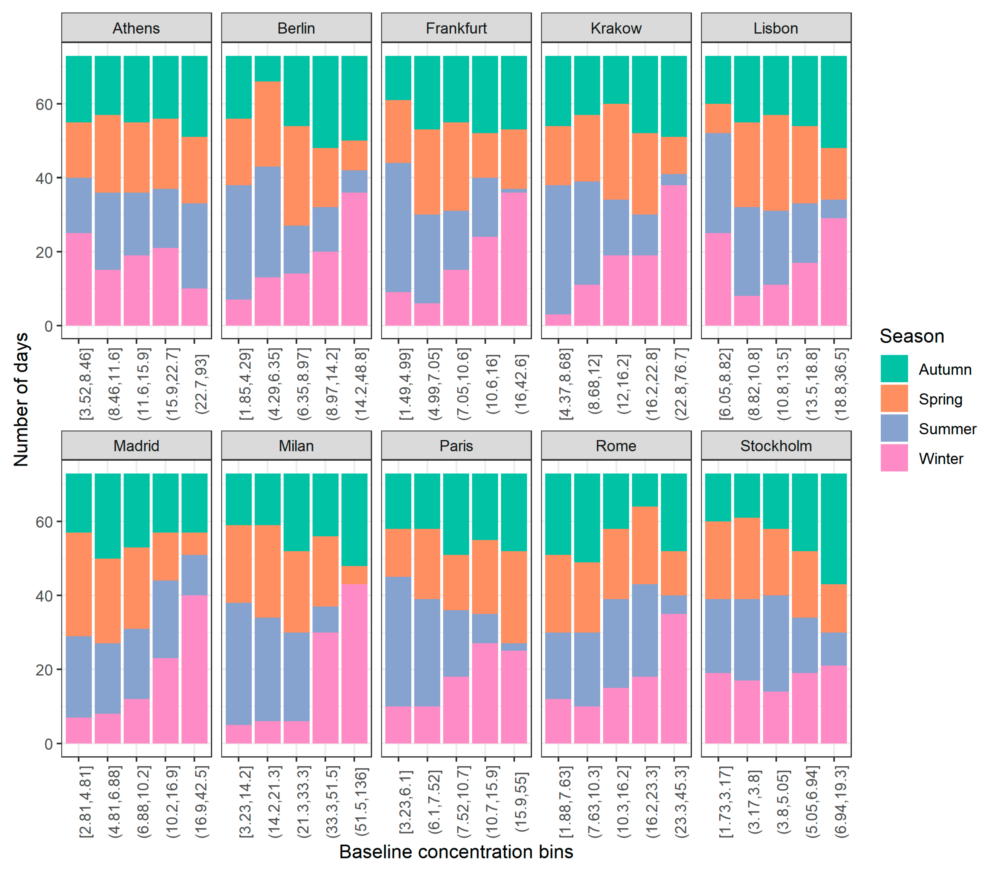
3.2.2. Yearly vs. Seasonal Results
Figure 4 proposes a similar analysis to
Figure 3, but with the results aggregated seasonally. As expected, the highest concentration bins mainly occur during winter in most cities (e.g., Berlin, Frankfurt, Krakow, Madrid, Milan, Rome). However, in other cities, this is less contrasted (Athens, Lisbon and Stockholm) and autumn is also a relevant season for high pollution episodes. For Paris, spring is very important in terms of high pollution episodes due to ammonium nitrate formation enhanced by fertilizer spreading in neighbouring regions and countries [
25].
3.2.3. Centroid vs. Hot-Spot Receptor
Figure 5 and
Figure 6 show similar results to
Figure 3 and
Figure 4, but for the second receptor choice corresponding to the ‘highest concentration point’ within the FUA.
With the focus on the ‘highest concentration point’, Lisbon and Stockholm can do much more with local actions, reducing up to 50% of their concentrations (while for the ‘centroid’ receptor, contributions were limited to roughly 25%). For both cities, the impact slightly decreases when considering higher concentration bins, but still remain high. Milan, on the contrary, shows an opposite behaviour with a city contribution that is reduced significantly to about 25% for the highest concentration bin, in contrast to 40–50% when considering the centroid. This is explained by the PPM emissions around the two points, that are 2.6 higher when focusing on the centroid, in contrast to the emissions close to the highest concentrations point; this emission issue is then causing different behaviours in the two cases, with higher local contributions when considering the centroid of the city (see
Supplementary Materials for this analysis). Southern cities like Lisbon, Madrid and Athens display a larger ’remaining’ contribution (i.e., from the boundary conditions mainly driven for particulate matter by Saharan desert dust). This is particularly noteworthy for Madrid during the high pollution episodes.
These results show the importance of the receptor point for the analysis of the policy impact as stressed in [
26].
3.3. Nonlinearities and Temporal Trends Assessment
Our methodology to evaluate the contribution of different sources on concentrations is based on full emission reductions (i.e., 100%) for all source areas (i.e., city, urban, agriculture…).
To evaluate the applicability of our approach to low and moderate (more realistic) emission reductions, we check here the importance of nonlinearities. We perform simulations with intermediate intensity emission reductions.
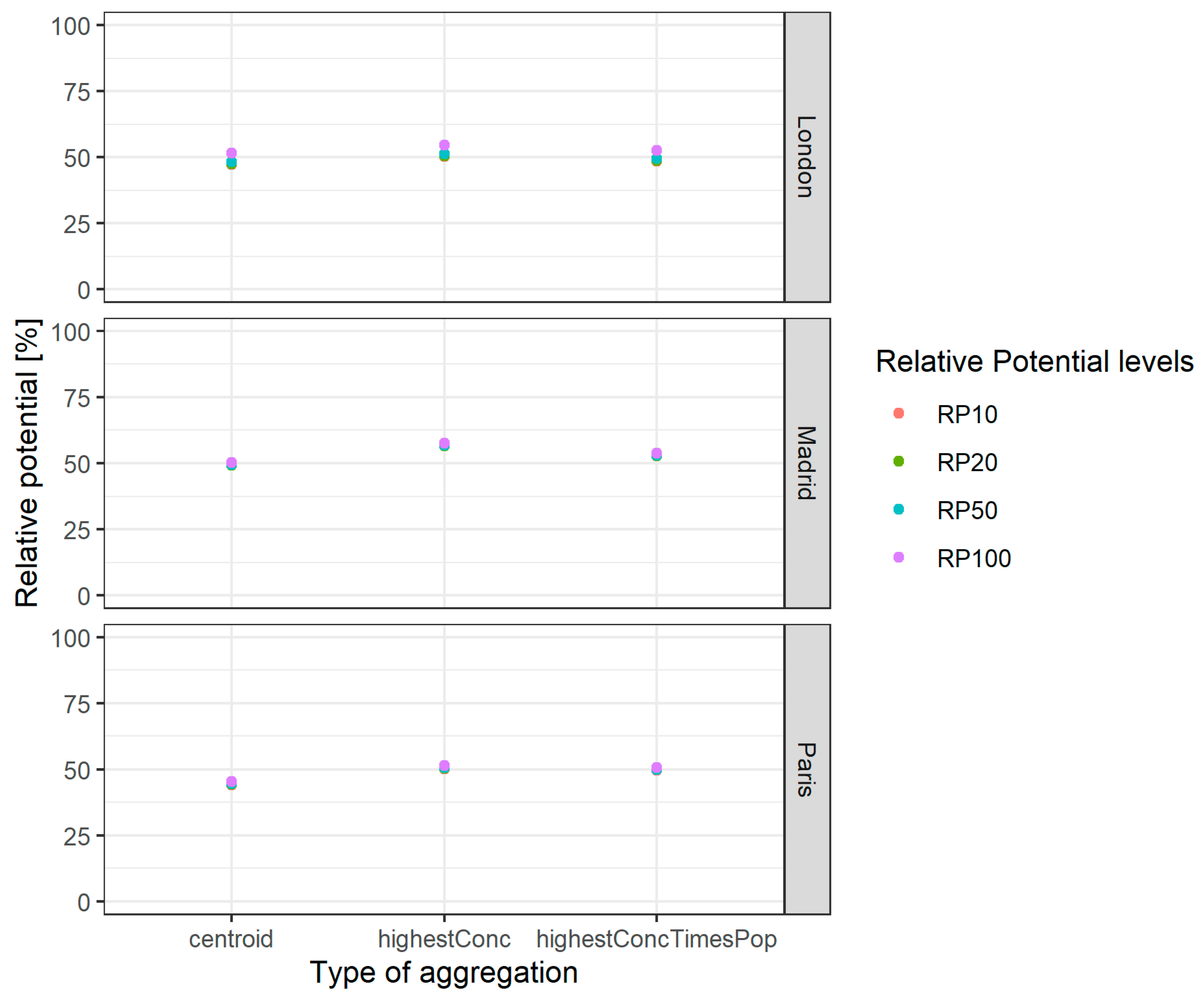
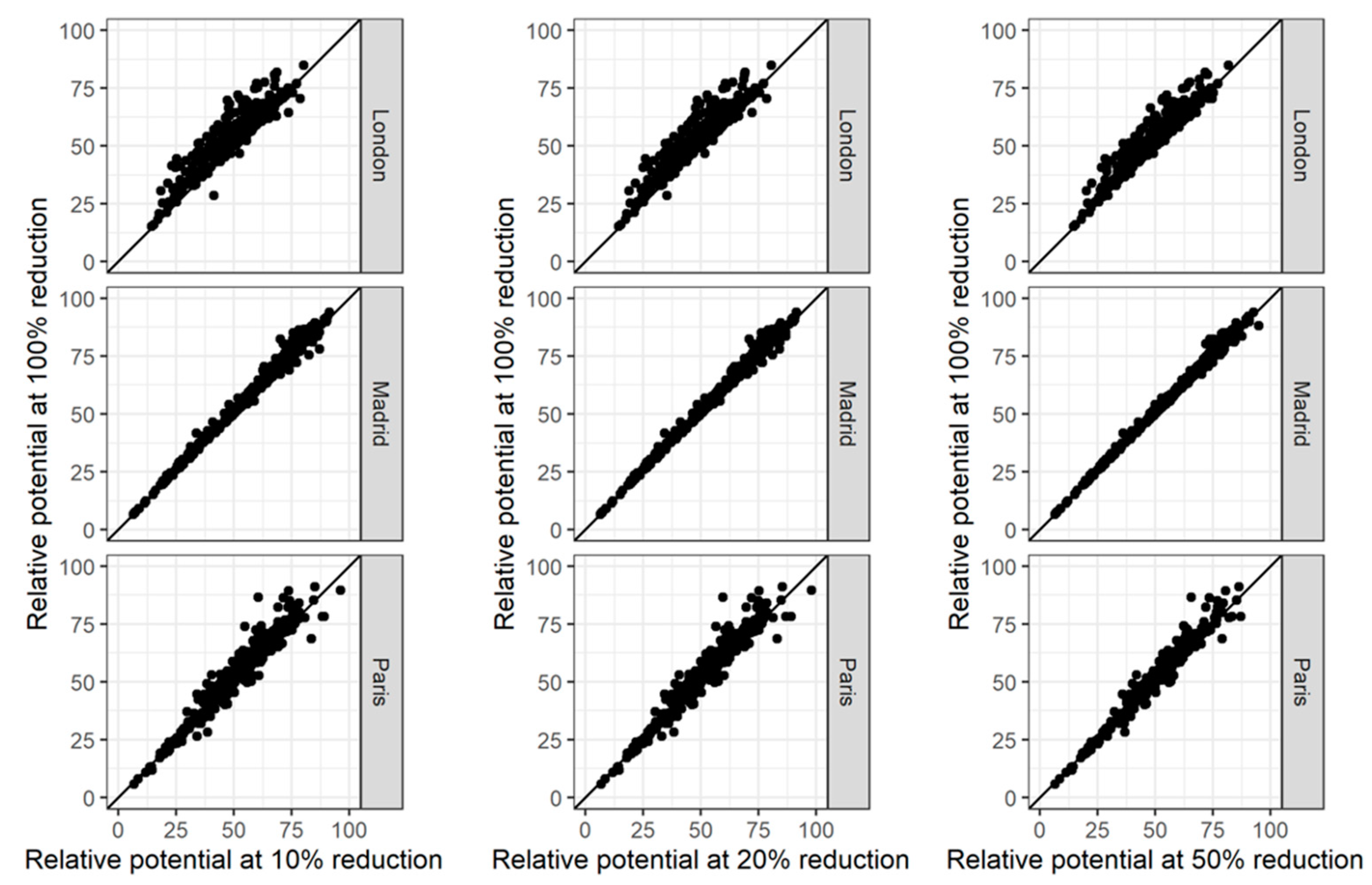
We simulated scenarios in which city emissions are reduced by 10%, 20% and 50% in three cities), and computed the associated relative potentials for the yearly, monthly and daily values. In the case of linear behaviour, relative potentials remain constant with the emission reduction intensity.
For the three considered cities (London, Madrid, Paris), the yearly average relative potential is shown in
Figure 7, for emission reductions of 10% (RP10), 20% (RP20), 50% (RP50) and 100%. There are not big differences for yearly averages, meaning that concentration changes due to 100% emission reductions (potential 100) are similar to twice the concentration changes due to 50% emission reductions (all ‘dots’ overlap), regardless of the receptor choice (the same stands when rescaling the cases at 20% or 10% reductions, that is to say rescaling RP20 and RP10).
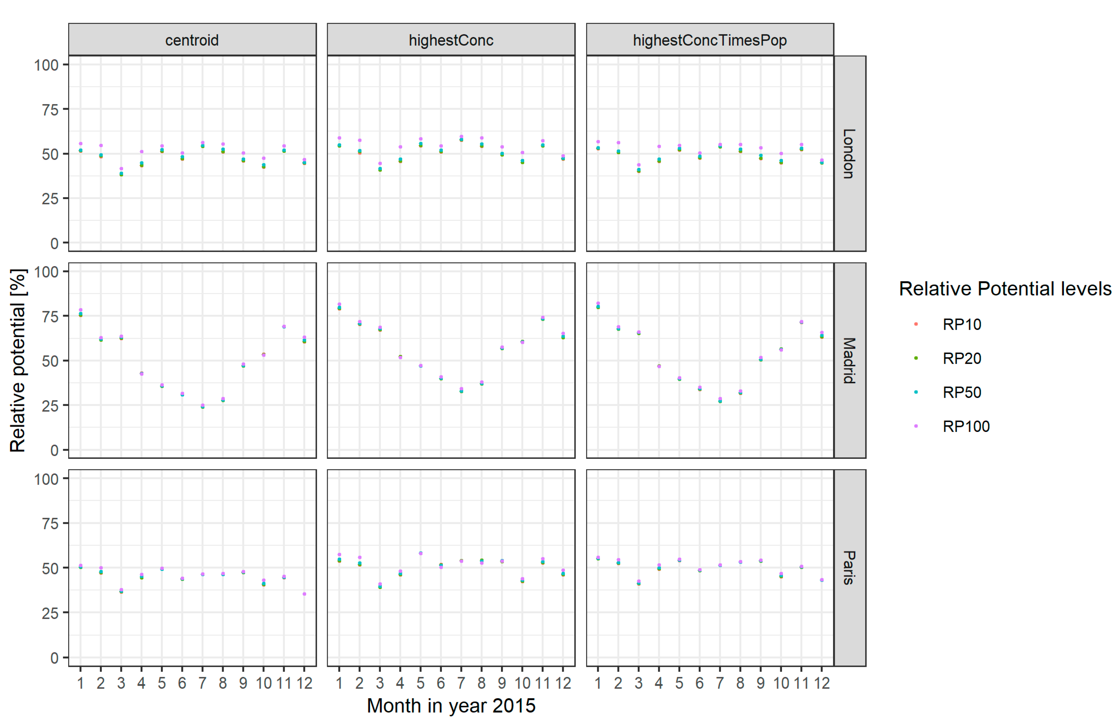
On top of this, we also checked temporal trends, and possible related nonlinear features. For monthly values (
Figure 8), relative potentials obtained for reductions ranging from 10% to 100% remain very similar, emphasizing the robustness of the approach. It is interesting to note the strong variability of the monthly trends in Madrid, moving from 75% (in winter) to 25% (in summer), while for London and Paris, the patterns are quite flat. The monthly trends in London and Paris are similar, with a limited variability; on the contrary, Madrid shows a more pronounced variability. This means that, focusing on plans that could be seasonally adapted would be of interest in Madrid, but not necessarily in the other two cities.
Even for daily values (
Figure 9), the 100% relative potential (y-axis) remains comparable to the potentials obtained for the 10%, 20% and 50% emission reductions (x-axis), at least for these three cities. In a previous work [
27], the nonlinear signal was more visible than here. In that work [
27], reductions were completed one pollutant at a time and on larger regional domains; in that case, the nonlinear trends were appearing at monthly, and increasing at daily, frequencies. In this study, the low nonlinear signal is probably lower due to the fact that reductions are performed on a smaller domain (city scale), reducing all pollutants at the same time.
4. Conclusions
In this work, we proposed a methodology to evaluate, for different cities, the effectiveness of local actions to reduce PM2.5 concentrations. The focus is on PM2.5, as it is the most complex pollutant to be managed at local scale, but also the one leading to the largest burden on human health [
15].
The traditional approach to evaluate the effectiveness of local actions is to use models in the scenario mode and assess what would happen with the implementation of local action plans, during specific short periods. In this work we use a different approach, consisting of running a set of simulations, on top of the baseline, and switching off different sources of emissions to understand how different cities react to different ‘sources’ of emission reductions, depending on the pollution level. So, the focus of this study is not on a specific episode, but more in general on the effectiveness of measures at different concentration levels.
The results (with an analysis of 10 cities) show that the concentration changes (linked to the considered scenarios) differ depending on the city; in particular, we can have cities where local actions are very effective for a high level of concentrations, and other cities that show an opposite behaviour. The analysis performed for two different receptor points within the city domain (‘centroid’ vs. ‘highest concentration’ point) showed that policy interventions can also vary significantly, depending on where the analysis is made (i.e., the selected receptor).
The generalisation of the findings to more realistic emission reductions has been tested by looking at how results change when modifying the level of emission reductions. The conclusion is that the methodology is robust, i.e., that similar results would be obtained for lower levels of emission reductions (e.g., 10%, 20% or 50%).
The overall conclusion of this work is that cities can generally improve, significantly, the pollution level through local actions during high-level concentration episodes, for PM2.5 (and also NO2). This is not the case for O3, which exhibits a completely different pattern. However, for PM2.5, in many cases an approach that only looks at local policies is not sufficient, and an integrated approach (through coordinated actions with other urban areas and/or acting on rural area emissions, etc.) would be needed. Finally, we suggest that, prior to the selection of a final action plan, a sensitivity is performed for different receptor points within the domain of interest, to ensure the most efficient policy. Indeed, given the large observed differences in terms of the receptor, averaging the results in terms of the receptor would lead to masking these geographical specificities and to lowering the impact of local strategies. In terms of limitation, the main uncertainty of this study lies in the EU wide emissions that could differ from locally reported ones. This aspect can affect the quality of the results, even if the general methodology would remain valid.


