Combining Numerical Simulations, Artificial Intelligence and Intelligent Sampling Algorithms to Build Surrogate Models and Calculate the Probability of Failure of Urban Tunnels

Abstract

When it is necessary to evaluate, with a probabilistic approach, the interaction of urban tunnels with neighboring structures, computational power is an important challenge for numerical models. Thus, intelligent sampling algorithms can be allies in obtaining a better knowledge of the result’s domain, even if in possession of a smaller number of samples. In any case, when sampling is limited, the evaluation of the risks is also restricted. In this context, artificial intelligence (AI) can fill an important gap in risk analysis by interpolating results and generating larger samples quickly. The goal of the AI algorithm is to find an approximation function (also called a surrogate model) that reproduces the original numerical simulation behavior and can be evaluated much faster. This function is constructed by performing multiple simulations at special points obtained by intelligent sampling techniques. This paper used a hypothetical case to validate the methodological proposal. It concerns the sequential excavation of a tunnel, about three diameters deep, interacting with a seven-story building. First, the three-dimensional numerical model (FEM) was solved deterministically, and then its domain and mesh were refined. After that, another 170 solutions were numerically obtained from FEM software, strategically sampling the random variables involved. Sequentially, based on 31 artificial intelligence techniques, it was evaluated which variables were of greatest importance in predicting the magnitude of vertical displacement in the foundation elements of a surrounding building. Then, once the most important variables were selected, the 31 artificial intelligence techniques were again trained and tested to define the one with the least R-squared. Finally, using this best-fit algorithm, it was possible to calculate the probability of failure using massive samples, with sizes on the order of ${10}^7$. These samples were used to illustrate the convergence of the Simple Monte Carlo Sampling (MC) and Latin Hypercube Sampling (LHS). The main contribution of this paper is methodological; therefore, this new procedure can be aggregated to state-of-the-art risk assessment methodologies in tunnel-related problems.

1. Introduction

The demand for underground space occupation has been significantly increasing, especially in urban centers, due to the growing relevance that humanity has been attributing to a walkable environment. In recent years, segregating elements, such as roads and viaducts, have been replaced by underground alternatives. As part of recent revitalization strategies, directing surface use of urban centers primarily toward work, housing and recreation is a tendency. Activities that do not align with these concepts, especially those related to traffic and storage, must occur mainly in underground spaces.

In this regard, tunneling techniques are good candidates to push the traffic of combustion-engine vehicles away from housing and commercial areas, providing a more walkable and vivid urban environment. This will, ultimately, increase life quality in these areas, in addition to inducing a healthier lifestyle (active mobility and less combustion-engine emissions nearby people). Therefore, tunneling techniques can be part of the strategy to revitalize large centers and, consequently, an improvement in the population’s quality of life.

Urban tunnels, in general, are excavated in soft ground with low geomechanical competence and low overburden, producing a relevant impact on nearby structures. In these cases, modeling and understanding the interaction between excavation procedures and the ground is usually challenging. Thus, among other factors, the construction techniques must consider the stability of the tunnel and the acceptable settlements in the affected neighboring structures.

The impacts caused by the excavation should be measured by a monitoring system, allowing for the identification of risks arising from tunnel construction. Mair et al. (1996) [1] proposed a methodology for the classification of hazards in neighboring structures. Based on this proposal, it is possible to adopt preventive measures that lead to greater safety and probability of success. As additional contributions, Ghorbani et al. (2012) [2], Pamukcu (2015) [3], and Huang and Zhang (2015) [4] emphasize the importance of monitoring excavations in urban areas. More recently, Liu et al. (2018) [5] proposed a numerical and probabilistic approach in a case study of the Wuhan subway in China.

Risk is inherent to all engineering works and can be understood as the chance of an event, beneficial or harmful, impacting the initially proposed objectives. For the geotechnical area, the publication of Whitman (1984) [6], almost 40 years ago, stands out as an important step in treating the risk theme in the decision-making process. In the present research, the focus will be on the negative consequences of a given event. Furthermore, in practical terms, the risk metric is defined as the product between the probability of failure and the subsequent consequences arising from this event.

The consequences of a failure at a tunnel construction site are strictly related to local conditions and must be analyzed on a case-by-case basis. This requires assessing the direct and indirect impacts of the failure and then transforming the effects into quantitative measures or, preferably, a financial impact.

On the other hand, evaluating the probability of failure is somewhat case-independent, allowing researchers to propose methodologies that can be applied to specific cases with only slight modifications. In this context, this research presents a new methodology that can be used during the risk assessment of urban tunnels, with special emphasis on the calculation of the probability of failure.

Normally, since analytical solutions rarely are applicable to real-world cases in this context, the starting point comprises the execution of numerical simulations. In a risk assessment framework, considering the high computational effort required by the combination of numerical analysis and statistical methods, an optimization of this process, with artificial intelligence, will be the core of the current study and, therefore, treated in greater depth in the following sections. Its benefits over current similar approaches will be discussed in the next sections. To consolidate theoretical knowledge and illustrate the application of the methodology, a practical application of the concepts in a hypothetical case is presented. It is highlighted how the proposed methodology enables a quantitative risk analysis that balances computational effort (processing time) with precision and accuracy.

This paper is organized as follows: a literature review is presented in Section 2. On the other hand, the new methodological framework is proposed in Section 3. To apply the concepts discussed, a hypothetical case and its deterministic numerical modeling are presented in Section 4. The discussions regarding the applicability of the new methodology, especially in parts where artificial intelligence and intelligent sampling algorithms are used, are presented in Section 5. Finally, the conclusions are presented in Section 6.

2. Evaluation of the Probability of Failure

As described, studying the interactions between the tunnel and the surrounding buildings has drawn much attention over the last decades. Crombecq et al. (2011) [7] report that to reduce the overall time, cost and/or risk, many modern engineering problems rely on accurate high-fidelity simulations instead of controlled real-life experiments. Such simulations can be used to understand and provide insights into the behavior of the system under study and to identify interesting regions in the design space. Furthermore, by varying the input parameters and observing the output results, it is also possible to understand the relationships between the different input parameters and how they affect the outputs [7].

This digital assessment of scenarios for a complex system with multiple inputs (also called factors or variables) and outputs (also called responses) can be a very time-consuming process, even for a single run [7,8].

This is not different for the analysis of shallow tunnels since the building of numerical models is needed, which tends to be computer intensive. The reader may refer to the works by Farias et al. (2004) [9], Guerrero (2014) [10] and Franco (2019) [11] for some examples. Therefore, optimizing the building process of a model is a key problem to address.

It is often desirable to perform a risk assessment of a given problem/engineering work. In this scenario, Wang et al. (2004) [12] report that quantitative probabilistic methods for uncertainty analysis include several steps, namely:

(a)

Quantifying and assigning probabilistic distributions to the input uncertainties,

(b)

Sampling the distributions of these uncertain parameters in an iterative fashion using Monte Carlo methods,

(c)

Propagating the effects of uncertainties through the model, and

(d)

Predicting the outcomes in terms of probabilistic measures such as mean, variance and fractiles.

Wang et al. (2004) [12] also indicate that the quality and consistency of the probabilistic analysis depend on the number of samples chosen, being this number ultimately defined for each analysis, as it depends on factors such as type of model, the random number generator used, type of distributions and the probabilistic output measure.

In general, the tendency is to reduce the samples as much as possible without impacting the decisions. As indicated by Wang et al. (2004) [12], to reach a similar accuracy, the mean of the output requires a number of samples that is an order of magnitude less than the number of samples required for the variance. Therefore, it is desirable to use a sampling technique that accurately predicts the output probabilistic measure with the minimum number of samples.

Crombecq et al. (2011) [7] indicate that some authors argue that the number of samples is much more important than the quality of the sampling design. They argue that it is obvious that the number of samples has an important effect on the quality of the model; on the other hand, practical and theoretical applications reveal that some sampling designs are better than others. Because every sample evaluation can potentially be very expensive, Crombecq et al. (2011) [7] propose that one must study the optimal location of a sample before submitting it for evaluation.

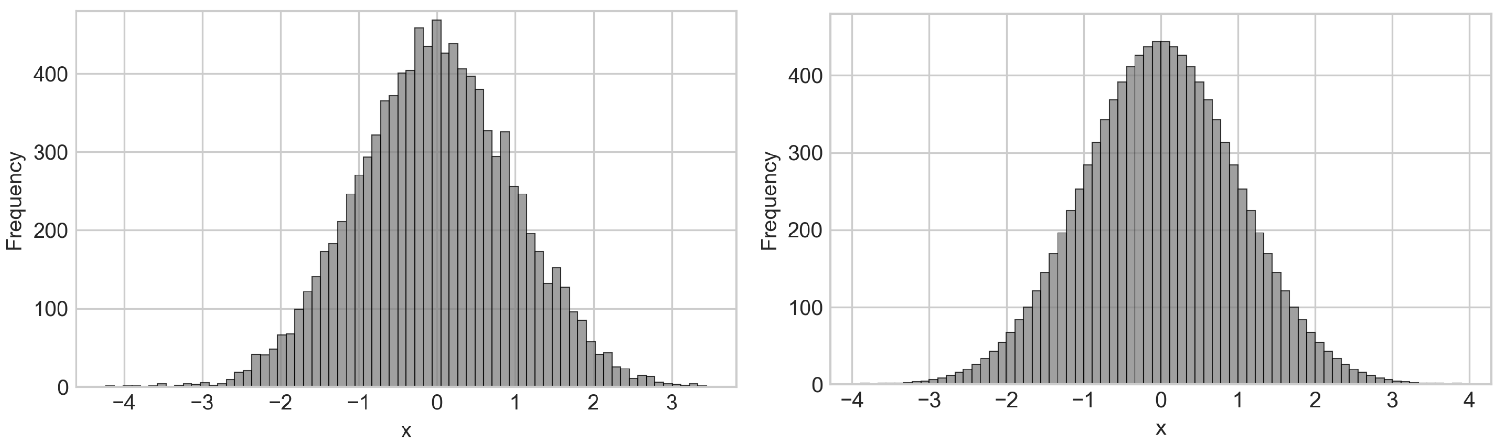
Similarly, Santos and Beck (2014) [13] present interesting results comparing standard Monte Carlo Sampling with the Latin Hypercube Sampling (LHS). In that publication, when comparing several intelligent sampling techniques applied to the Monte Carlo method, it was pointed out that results obtained after an LHS converge faster (fewer samples needed) while compared to standard sampling. This could be explained by the fact that the former provides a more homogeneous mapping of the domain. As an illustration, it is possible to analyze the frequency histogram proposed by Santos and Beck (2014) [13] for a normal random variable with a mean of 1.0 and standard deviation of 0.15, illustrated in Figure 1.

This way, not only the quantity but also where each sample is generated, can help optimize the probabilistic assessment of tunnel construction situations. In these situations, as indicated in step (a) [12], it is important to define which parameters of the numerical shallow tunnel model are not deterministic, i.e., they are random variables (RV). This normally can be performed by a literature review on the behavior of each parameter.

For example, one can look for the statistical distributions and coefficient of variation (CV) values reported for each parameter. Since the CV indicates the relative magnitude between the mean and the standard deviation values of a given RV, parameters with low CV (close to zero) tend to be well modeled as deterministic variables. The works of Srivastava and Sivakumar Babu (2009) [14], Kayser and Gajan (2014) [15] and Grasmick et al. (2020) [16] present important discussions on this subject.

Another step in this RV identification is to assess which variables are important for the particular problem being studied. Sometimes, the spatial arrangement and conditions of the problem may allow disregarding a few RVs based on their relative influence on the specific result under analysis. For example, the constitutive parameters of a deep layer of soil could have low or no impact on the behavior of shallow tunnels. This process is important to target the simulations to account only for what really impacts the final result, avoiding unnecessary runs of the numerical algorithms. There are several methods in the literature for this sensitivity/feature selection analysis, such as the First Order Second Moment (FOSM) [17] and Tornado diagram analysis [18]. Overall, we can say that the relative importance of a given RV relies on its direct mathematical impact on the formulation of the engineering problem as well as on its CV (even low CV variables can be important).

After this random variable identification process has been carried out, it is important to sample these RV according to a proper technique, as described in step (b) above. The sampled values are then used to run the deterministic numerical models, producing a set of results that reflect the variability of the input parameters, as pointed out in steps (c) and (d).

Mathematically, it can be said that $X_i$, $i=1,...,n$ are the input random variables of an n-parameter simulation. In this study, the output is assumed to be a known deterministic function $d\left(X\right)$ whose argument is a vector with samples $X_i^{\left(s\right)}$ of each of the RV inputs, $X=[X_1^{\left(s\right)},X_2^{\left(s\right)},...,X_n^{\left(s\right)}]$.

Normally, a Monte Carlo approach would end here, calculating the failure probability based on the set of results. As previously indicated, this may not be possible to achieve as the number of simulations required for accurate calculations of the probability of failure is prohibitive for more complex numerical models, which can take up to several days to run.

Therefore, this proposed methodological procedure does not consider the calculation of probabilities of failure based on this set of results. Instead, these results are used to calibrate an Artificial Intelligence algorithm capable of learning from them and predicting new results from different input parameters. This calibrated algorithm is used as a substitute for the numerical model trying to mimic it. Therefore, it can be run several millions of times in a fraction of the time taken to run the real numerical model. In other words, in this framework, an AI model $d^{AI}\left(X\right)$ is trained to replace the numerical model $d\left(X\right)$, allowing for multiple evaluations in seconds. This will allow the generation of massive sets of results, which can be properly used to evaluate the probability of failure even in “brute” Monte Carlo scenarios.

To properly calibrate the AI algorithm, the RVs need to be sampled accordingly. In addition to standard sampling techniques, the literature reveals several enhanced procedures that attain many benefits. Since building an AI surrogate model is aimed, Crombecq et al. (2011) [7] point out that the creation of an approximation model that mimics the original simulator is needed, based on a limited number of expensive simulations but that can be evaluated much faster.

If the understanding of how the numerical algorithm behaves for multiple input parameters is desirable, it is necessary to sample these parameters to cover the whole input domain as much as possible. The sampling points must be informative key points in the design space, such that the overall system behavior is approximated quite well [7,19,20]. This can be achieved with the so-called space-filling techniques, which try to sample a multidimensional domain in a way that every subdomain is almost equally sampled too. These techniques can be easily implemented and provide a good (and guaranteed) coverage of the domain. Popular space-filling designs are fractional designs [21], Latin hypercubes [22] and orthogonal arrays [23].

By selecting a space-filling technique, it is sure that the AI algorithm will learn from a set of values that truly represent the whole domain, being able to produce accurate results for unseen data. After this intelligent technology is used, the AI algorithm is trained. The recent work by Ji et al. (2021) [24] presents a similar approach to building surrogate models in a slope system reliability scenario.

Artificial intelligence methods are gaining attention in several areas of knowledge due to their capabilities and adaptability. Shreyas and Dey (2019) [25] investigate the applicability in tunneling-related problems, exploring the techniques of artificial neural networks (ANN), radial basis functions (RBF), decision trees (DT), random forest (RF) method, support vector machines (SVM), nonlinear regression methods such as multi-adaptive regression splines (MARS), and hybrid intelligent models. Emphasis should be placed on artificial neural networks (ANN), capable of modeling nonlinear relationships between multiple input and output variables. Moreover, this technique has already been applied to a range of tunneling studies, such as Suwansawat and Einstein (2006) [26], Zhang et al. (2017) [27], Yang and Xue (2017) [28], Zhang et al. (2019) [29] and others. In addition, other simpler techniques such as decision trees have also had their application validated in tunnel-related problems, as exposed by Shahriar et al. (2008) [30], Dindarloo and Siami-Irdemossa (2015) [31], Mohmoodzadeh et al. (2020) [32] and others.

In addition to being capable of creating surrogate models, AI algorithms can also be used to select which RVs are important for our specific problem. In order to do so, recursive feature elimination with cross-validation (RFECV) techniques can be used to select the number of features that really affect the output.

This way, in the next section, a methodological framework is explored, which combines numerical simulation, AI techniques and intelligent sampling techniques to build a surrogate model for studying the vertical displacements induced by shallow tunnel construction.

In particular, these vertical displacements are later used to calculate the angular distortion between the foundation elements. Several authors listed in Foá (2005) [33] use the angular distortion parameter to study the impact of tunnels on buildings.

Table 1. Building damage as discussed in [34].

Damage Criteria	Angular Distortion ($\mathsf{\beta }=\mathsf{\delta }/\mathbf{L}$)
Machinery sensitive to settlements are to be feared	1/750
Danger for frames with diagonals	1/600
Safe limit for buildings where cracking is not permissible	1/500
First cracking in panel walls is to be expected	1/300
Difficulties with overhead cranes are to be expected	1/300
Tilting of high, rigid buildings might become visible	1/250
Considerable cracking in panel walls and brick walls	1/150
Limit for flexible brick walls, h/L < 1/4	1/150
Structural damage of general buildings is to be feared	1/150

presents some damage criteria discussed by Burland and Wroth (1974) [34], where the angular distortion $\beta$ is defined by the ratio between the differential settlement $\delta$ and the distance between the measurement reference points L. This distortion indicator was chosen for methodological validation and, in any case, changing the indicator would not invalidate the methodology hereby proposed. Other methods of damage assessment based on angular distortion and extension deformation are also available, but, for simplicity, this tabular approach has been chosen in the present paper.

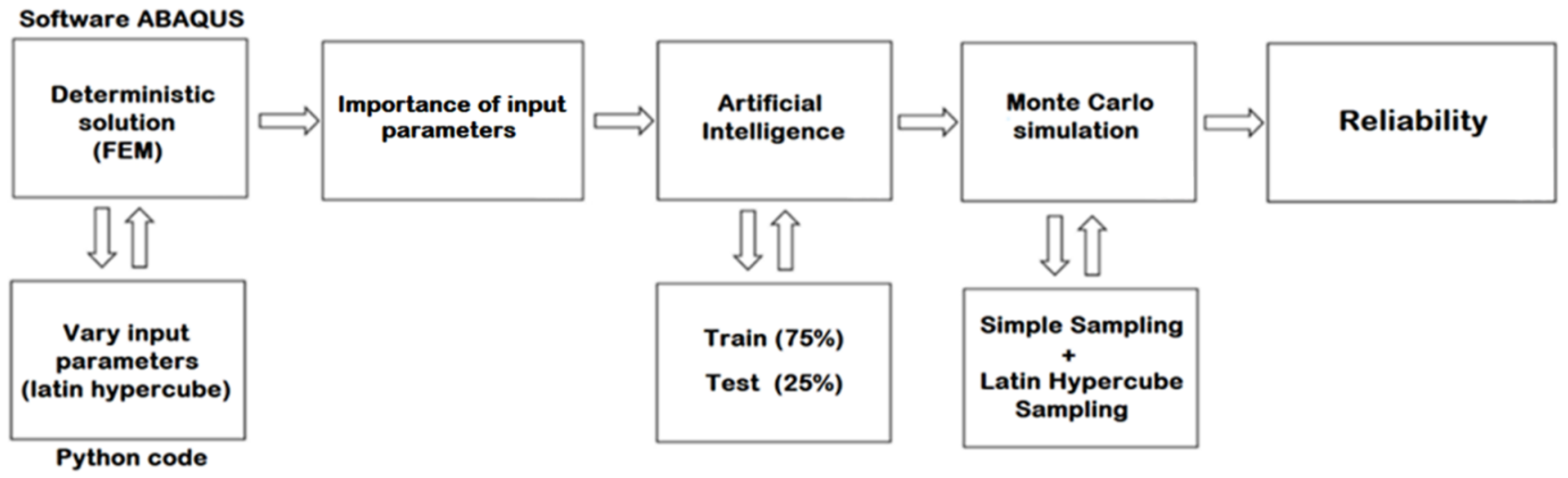
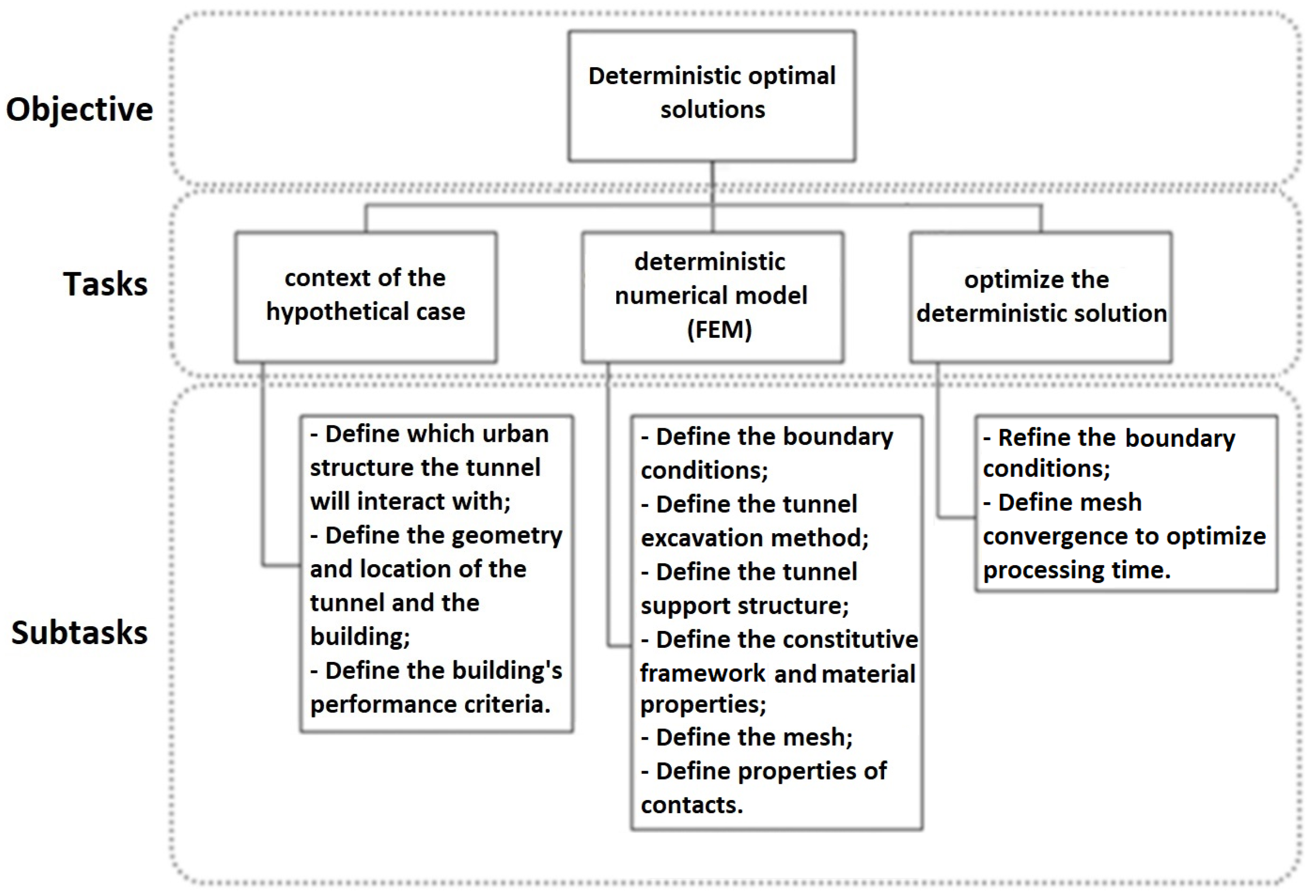
3. Proposed Methodology

This section presents the proposed methodological framework for calculating the probability of failure, making use of numerical simulations, artificial intelligence techniques and intelligent sampling algorithms. The proposed process is presented in Figure 2 and detailed in the following subsections.

3.1. Deterministic Solutions Used to Build Surrogate Model

The deterministic solution was obtained with the aid of the FEM software ABAQUS. This software was combined with a Python code to enable sampling the random input variables and directly building the input files needed for the simulations. As discussed in Section 2, the Latin Hypercube Sampling method presented a good space-filling capability and was used to obtain a general knowledge of the input/output values.

This way, it was necessary to import the Latin Hypercube Sampling algorithm (LHS) implemented in the skopt Python package (in special, from the ‘skopt.sampler’ methods). The ‘centered’ type (where points are set uniformly in each interval) and the ‘maximin’ criterion (where an optimized LHS is implemented by maximizing the minimal difference between all the points sampled) were used.

The literature indicates that in order to calibrate meaningful multi-variable regressions, on average, samples need to be from 10 [35] to 30 [36] times the number of input variables. This minimum number of samples is also severely impacted by the correlation between the variables considered [37].

In the case of the present study, the vast majority of Geotechnical Engineering literature presents several empirical relations between constitutive parameters. For example, Kumar et al. (2016) [38] indicate that the number of blows in the Standard Penetration Test (NSPT) can be used to predict the Young’s modulus, cohesion and friction angles of soils. Therefore, this suggests a high correlation between these variables. In addition, it is also known that $k_0$ can be related to the friction angle [39,40], which again indicates that the input variables considered in the present paper are highly correlated.

It is important to highlight that both positive and negative correlations have similar impacts in this particular discussion. The general idea is that, for two random variables X and Y, one can be interpreted as a function $f(.)$ of the other, $Y=f\left(X\right)$. The function’s trend can be either increasing or decreasing, therefore allowing for a positive or negative correlation. Previous studies have also suggested that effective cohesion and effective friction angle can be negatively correlated [41], which also reinforces the correlation of the variables studied in the present paper.

Thus, by considering that the Young modulus, cohesion and friction angles are correlated, it is possible to suppose that the independent input variables drops from 34 to 26 (4 friction angle and 4 cohesion random variables are dependent). Now, by considering that $k_0$ is dependent on the friction angle (which is dependent on the Young’s modulus as a proxy for NSPT), the number of independent random variables drops from 24 to 20. Finally, by noticing that Lame’s formula indicates that both the Young’s modulus and Poisson ratio are dependent, the number of input variables drop from 20 to 14. Other possible dependencies could be investigated, such as between density and friction angles, but for simplicity, the reduction stopped in 14 independent random variables.

This way, in theory, it would be necessary to generate 140 to 420 samples if all the independent variables were effectively needed to explain the output quantity (displacement at the toe of a foundation element). For simplicity, 170 samples (about 12 times the number of independent input variables or 5 times the number of dependent input variables) were generated in the present paper. This assumption will be shown to be effective, as the number of explanatory variables considerably dropped after the variable selection stages.

Considering the computational processing time to generate and store all ABAQUS results, the routine proposed in Python also performed the duty of specifically collecting stresses and displacements for specific mesh nodes. As part of the routine, a datasheet file (“.xlsx”) was generated for each simulation to allow the results to be easily consulted later.

The lower boundary and upper boundary of the sampling intervals for each random variable must be defined to match the smallest possible value for the parameter and the 95% percentile value, respectively.

In order to perform any optimization on the domain of the finite element model, a good approximation is to consider that the lowest geomechanical strength parameters represent the critical condition (lower boundaries of the sampling intervals, if positively correlated to the strength of the model). Thus, these parameters can be adopted in the first model of the finite element solver to find the optimized domain and mesh.

3.2. Input Parameter Selection by Artificial Intelligence Techniques

As described, the relative importance of input parameters can be evaluated by means of the sklearn Python^® package and its implemented method known as RFECV, which handles recursive elimination of variables with cross-validation. This method allows to find the informative input variables for a given AI algorithm by means of a recursive procedure, where features are iteratively removed and then the best subset of features is chosen based on the cross-validation score of the model. Particularly, sklearn’s algorithm begins the process with a model that includes all variables and then assigns an importance score to each one. Next, the random variables of lesser importance are removed, the model is reconstructed, and the importance scores are recalculated. In the present paper, for each iteration of the RFECV method, a single feature was removed after a 5-fold cross-validation strategy was considered (model parameters ‘step = 1, cv = 5’). Thus, the result of this analysis can lead to a reduction in the number of random variables involved in the problem.

Instead of selecting only one regressor algorithm to use the RFECV method, it was chosen to perform a voting strategy, where several techniques were applied and each parameter received a vote whenever it was selected as a relevant feature for the model. By using the Python sklearn library, the authors gathered all the available regressor-type estimators by importing the method “all_estimators” from “sklearn.utils” and obtaining the available estimators as “all_estimators(type_filter=’regressor’)”.

This way, the techniques considered were [42,43]:

• Bayesian ARD regression (‘ARDRegression’),
• AdaBoost regressor (‘AdaBoostRegressor’),
• Bayesian ridge regression (‘BayesianRidge’),
• Canonical correlation analysis (‘CCA’),
• Decision tree regressor (‘DecisionTreeRegressor’),
• Elastic net regressor (‘ElasticNet’), which is basically a linear regression with combined L1 and L2 priors as the regularizer,
• Elastic net CV regressor (‘ElasticNetCV’), which is an elastic net model with iterative fitting along a regularization path,
• Extremely randomized tree regressor (‘ExtraTreeRegressor’),
• Extra-trees regressor (‘ExtraTreesRegressor’),
• Gradient boosting for regression (‘GradientBoostingRegressor’),
• Linear regression model that is robust to outliers (‘HuberRegressor’),
• Least angle regression (‘Lars’),
• Cross-validated least angle regression (‘LarsCV’),
• Linear model trained with L1 prior as regularizer (‘Lasso’),
• Lasso linear model with iterative fitting along a regularization path (‘LassoCV’),
• Lasso model fit with least angle regression (‘LassoLars’),
• Cross-validated lasso, using the LARS algorithm model (‘LassoLarsCV’),
• Lasso model fit with Lars using Bayes information criterion or Akaike information criterion for model selection (‘LassoLarsIC’),
• Ordinary least squares linear regression (‘LinearRegression’),
• Linear support vector regression (‘LinearSVR’),
• Orthogonal matching pursuit model (‘OrthogonalMatchingPursuit’),
• Partial least squares transformer and regressor (‘PLSCanonical’),
• Partial least squares regressor (‘PLSRegression’),
• Passive aggressive regressor (‘PassiveAggressiveRegressor’),
• Generalized linear model with a Poisson distribution (‘PoissonRegressor’),
• A random forest regressor (‘RandomForestRegressor’),
• Linear least squares with L2 regularization (‘Ridge’),
• Ridge regression with built-in cross-validation (‘RidgeCV’),
• Linear model fitted by minimizing a regularized empirical loss with Stochastic gradient descent (‘SGDRegressor’),
• Theil-Sen estimator (‘TheilSenRegressor’), which is a robust multivariate regression model,
• Generalized linear model with a Tweedie distribution (‘TweedieRegressor’).

No manual hyperparameter tuning was performed for these techniques. For some of the cases, mainly those with cross-validation, an automatic refinement is carried out. Furthermore, an ensemble methodology was considered by noticing that even weak predictors, when combined in a voting strategy, can lead to a robust global prediction of the important features [44].

It is important to highlight that a scaling of the input values was performed by using the function MinMaxScaler of the sklearn package, which scales and translates each feature individually such that it is in the given range on the training set (in our case, between zero and one). Finally, the top-voted parameters were chosen to build our optimized AI model. The top-voted parameters are understood as the parameters that were important to at least 50% of the regressor algorithms used.

3.3. Training and Testing Artificial Intelligence

After obtaining the optimal number of random input variables, all the artificial intelligence regressors used in the variable selection step were re-submitted to the training and testing process. For this training and testing process, about 75% of the samples (128 samples) were used for training and 25% (42 samples) for testing. The 31 previously indicated artificial intelligence regressors were trained and a first approximation would be to choose the algorithm with the highest accuracy in the testing stage. On the other hand, if the mean absolute error is much greater than 1mm (which is the displacement threshold we chose to optimize the finite element numerical model), it would be necessary to perform a parameter optimization for each algorithm. Furthermore, cross-validation should also be considered to exclude the influence of the sample set partition on the results.

3.4. Monte Carlo Sampling Techniques to Calculate the Probability of Failure: Simple and Latin Hypercube Sampling

After the validation of the artificial intelligence surrogate model, samples are generated for the Monte Carlo technique with simple sampling [45] and Latin hypercube sampling [46], allowing the comparison of these techniques.

When populating the input parameter space, the ‘centered’ and ‘maximin’ optimized LHS points were obtained by using the skopt Python package. The authors chose this specific implementation in order to better spread the input variables in their domain. On the other hand, the computational cost of the skopt implementation becomes considerably high as the number of samples increases. Since the present methodological step demands large samples, it is possible to relax the ‘maximin’ criterion and use a much simpler centered implementation of the LHS method. This low-cost implementation was performed using numpy, by noticing that an N-dimensional LHS sample of M variables can be generated by collecting M random permutations of the integers 0 through $N-1$. The resulting M × N matrix gives a list of coordinates that will form a Latin hypercube. By adding 0.5 to the coordinates indicated, this Latin hypercube becomes centered [47].

At this point, the probability density functions of each of the random input variables are defined and used in the sampling procedure. This is because, initially, they were disregarded to fill the domain homogeneously, according to the LHS.

In this methodological step, the recovery of the statistical distributions of the random variables is performed by the inverse transformation method. In this method, with possession of the cumulative distribution $F\left(x\right)$, uniformly distributed values y between 0 and 1 are used to recover samples x by the following formula $x=F^{-1}\left(y\right)$, where the superscript −1 indicates the inverse function.

To find the actual distribution parameters (scale and location) for each RV, a system of equations obtained by locking the coefficient of variation at certain values and using the 95% percentile constraint for the upper boundary of the sampling range (which was cited previously) was solved. This approach narrows the variability of the input variables to a known range and populates their domain in a way that only a few values will be sampled outside the pre-sampled values. This helps to keep generalization errors controlled, and almost no extrapolation is performed, as most of the time, the input variables are within a known pre-sampled range.

3.5. Reliability of Sampling Techniques

This last methodological step is not directly related to the creation of a surrogate model. Still, it is important to check how intelligent sampling techniques can be used to reduce the number of samples needed to calculate the probability of failure of a hypothetical shallow tunnel.

Considering the possibility of generating many samples in a short time, the probabilities of failure will be evaluated with the Monte Carlo techniques by simple sampling and LHS. In this convergence analysis, twelve input sample sizes will be evaluated, ranging from ${10}^2$ to ${10}^7$. The reference value for comparison will be the one obtained with the ${10}^7$ sample size of the standard Monte Carlo simulation, and the choice of twelve sample sizes is uniquely related to a visually admissible granularity of the log-plotted data and can be changed if desired.

Since partial sampling also includes uncertainties, the data will always be represented by statistical distributions. To define the distribution that gives the best fit to the results, eighty-four statistical distributions will be tested, all of which are presented in the scipy Python package, namely [48]: Alpha (‘alpha’), Anglit (‘anglit’), Arcsine (‘arcsine’), Beta (‘beta’), Beta prime (‘betaprime’), Bradford (‘bradford’), Burr type III (‘burr’), Burr type XII ‘burr12’, Cauchy ‘cauchy’, Chi (‘chi’), Chi squared (‘chi2’), Cosine (‘cosine’), Double gamma (‘dgamma’), Double Weibull (‘dweibull’), Erlang (‘erlang’), Exponential (‘expon’), Exponentially modified Normal (‘exponnorm’), Exponential power (‘exponpow’), Exponentiated Weibull (‘exponweib’), F (‘f’), Fatigue-life (Birnbaum-Saunders) (‘fatiguelife’), Fisk (‘fisk’), Folded Cauchy (‘foldcauchy’), Folded Normal (‘foldnorm’), Gamma (‘gamma’), Gauss hypergeometric (‘gausshyper’), Generalized exponential (‘genexpon’), Generalized extreme value (‘genextreme’), Generalized Gamma (‘gengamma’), Generalized half-logistic (‘genhalflogistic’), Generalized logistic (‘genlogistic’), Generalized Normal (‘gennorm’), Generalized Pareto (‘genpareto’), Gilbrat (‘gilbrat’), Gompertz (‘gompertz’), Left-skewed Gumbel (‘gumbel_l’), Right-skewed Gumbel (‘gumbel_r’), Half-Cauchy (‘halfcauchy’), Upper half of a generalized Normal (‘halfgennorm’), Half-logistic (‘halflogistic’), Half-normal (‘halfnorm’), Hyperbolic secant (‘hypsecant’), Inverted gamma (‘invgamma’), Inverse Gaussian (‘invgauss’), Inverted Weibull (‘invweibull’), Johnson SB (‘johnsonsb’), Johnson SU (‘johnsonsu’), Limiting distribution of scaled Kolmogorov-Smirnov two-sided test statistic (‘kstwobign’), Laplace (‘laplace’), Levy (‘levy’), Left-skewed Levy (‘levy_l’), Log gamma (‘loggamma’), Logistic (‘logistic’), Log-Laplace (‘loglaplace’), Log-normal (‘lognorm’), Lomax (Pareto of the second kind) (‘lomax’), Maxwell (‘maxwell’), Mielke Beta-Kappa or Dagum (‘mielke’), Nakagami (‘nakagami’), Non-central Student’s t (‘nct’), Non-central chi-squared (‘ncx2’), Normal or Gaussian (‘norm’), Pareto (‘pareto’), Pearson type III (‘pearson3’), Power-function (‘powerlaw’), Power log-Normal (‘powerlognorm’), Power Normal (‘powernorm’), Rayleigh (‘rayleigh’), R-distributed (symmetric beta) (‘rdist’), Reciprocal inverse Gaussian (‘recipinvgauss’), Reciprocal (‘reciprocal’), Rice (‘rice’), Semicircular (‘semicircular’), Student’s t (‘t’), Triangular (‘triang’), Truncated exponential (‘truncexpon’), Truncated Normal ‘truncnorm’, Tukey-Lamdba (‘tukeylambda’), Uniform (‘uniform’), Von Mises (‘vonmises’), Von Mises defined in (−$\pi$,$\pi$) (‘vonmises_line’), Wald (‘wald’), Weibull Maximum Extreme Value (‘weibull_max’) and Weibull Minimum Extreme Value (‘weibull_min’). Even though strictly positive distributions were not selected, the domain of the best fit distribution will be truncated to positive values if needed. This comes from the fact that the RV being modeled is the absolute value of the angular distortion.

Each distribution will be fitted by the maximum likelihood estimators for the set of ${10}^6$ standard Monte Carlo simulations, choosing the best distribution by combining their Akaike information criterion (AIC), introduced by Akaike (1974, 1983) [49,50], with the quadratic error of the fit (with respect to the empirical histogram). The sample size of ${10}^6$ was chosen because the general shape of the distributions is already defined with samples this large.

As pointed out by Maydeu-Olivares and García-Forero (2010) [51], the AIC is not used to test the model in the sense of hypothesis testing but for model selection. Given a data set, one can calculate AIC for all models under consideration. Then, the model with the lowest index is selected. This type of criterion combines absolute fit with model parsimony, penalizing models that provide a good fit at the cost of incorporating multiple parameters.

A combination of the AIC and the quadratic error criteria will be performed. The AIC ranking is paramount and is the first classification sequence to be followed. The quadratic error is only used to discard distributions with low AIC values but whose fitting ability is notably poor. This process of selecting the appropriate distribution is crucial to any probabilistic modeling of datasets [52]. After that, in the evaluation of other samples, the parameters of the chosen distribution will be estimated from the partial (smaller size samples) results.

4. Hypothetical Case of an Urban Tunnel

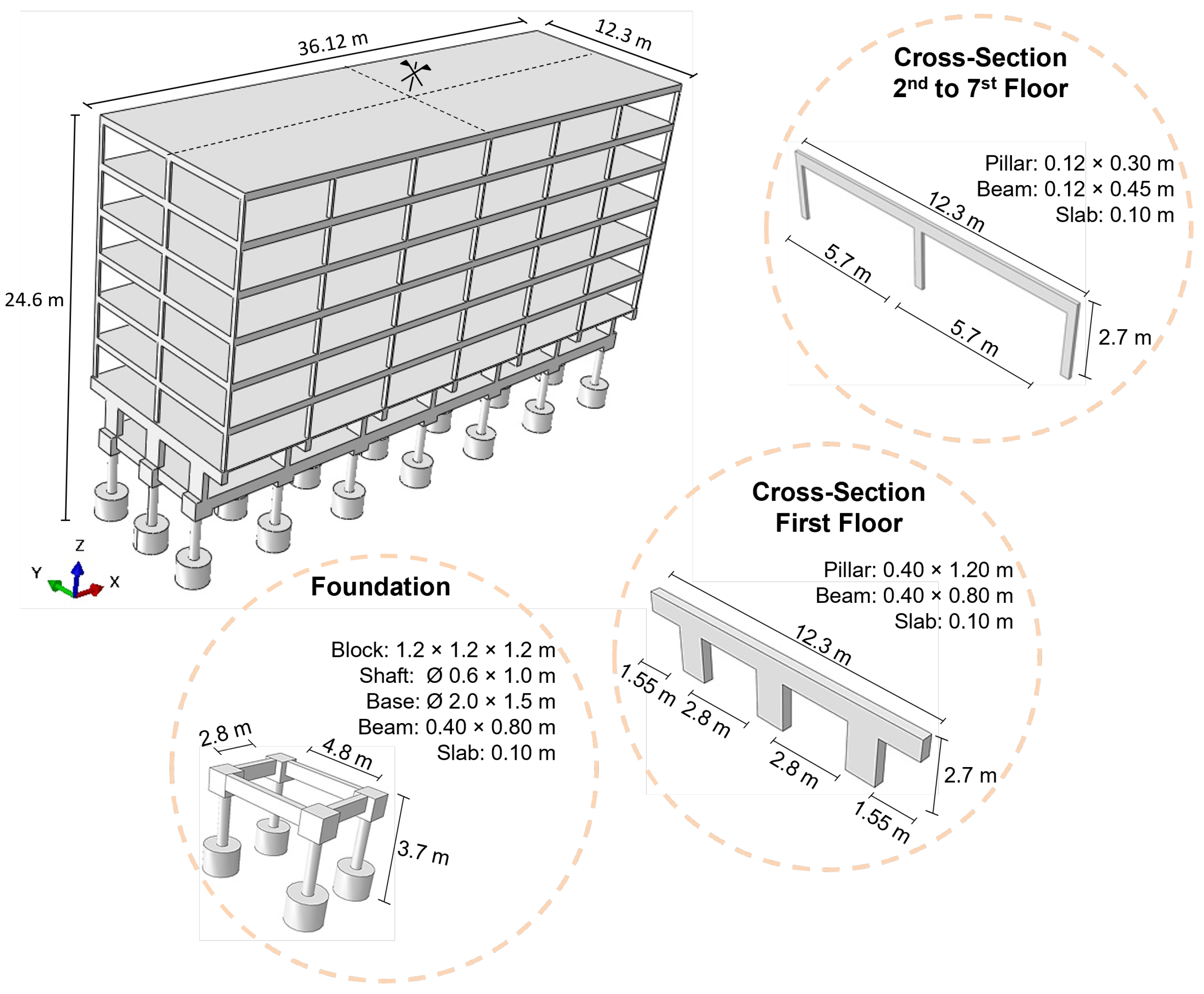
The hypothetical case seeks to reproduce a representative urban tunnel and, therefore, to validate the methodology for obtaining a surrogate model for vertical displacement and the probability of failure of surrounding buildings.

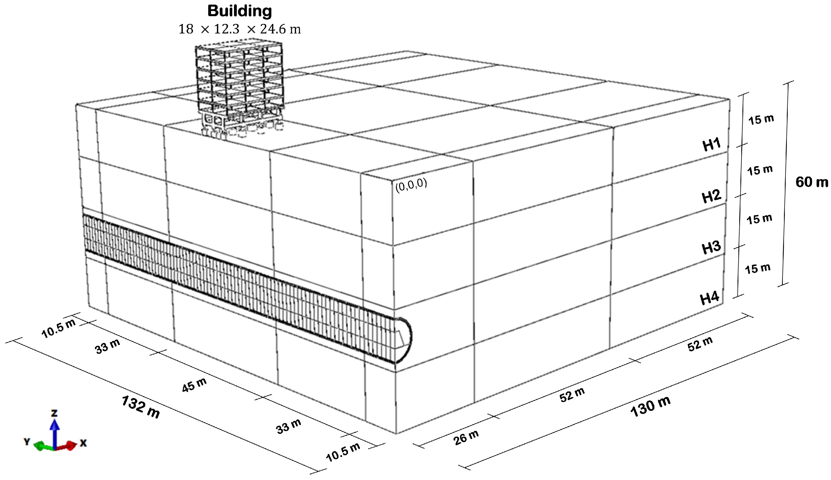
Thus, the case was based on the interaction between a tunnel excavated to a depth of three diameters and a building with seven floors. In this case, the performance of the building was analyzed regarding the serviceability limit state (SLS).

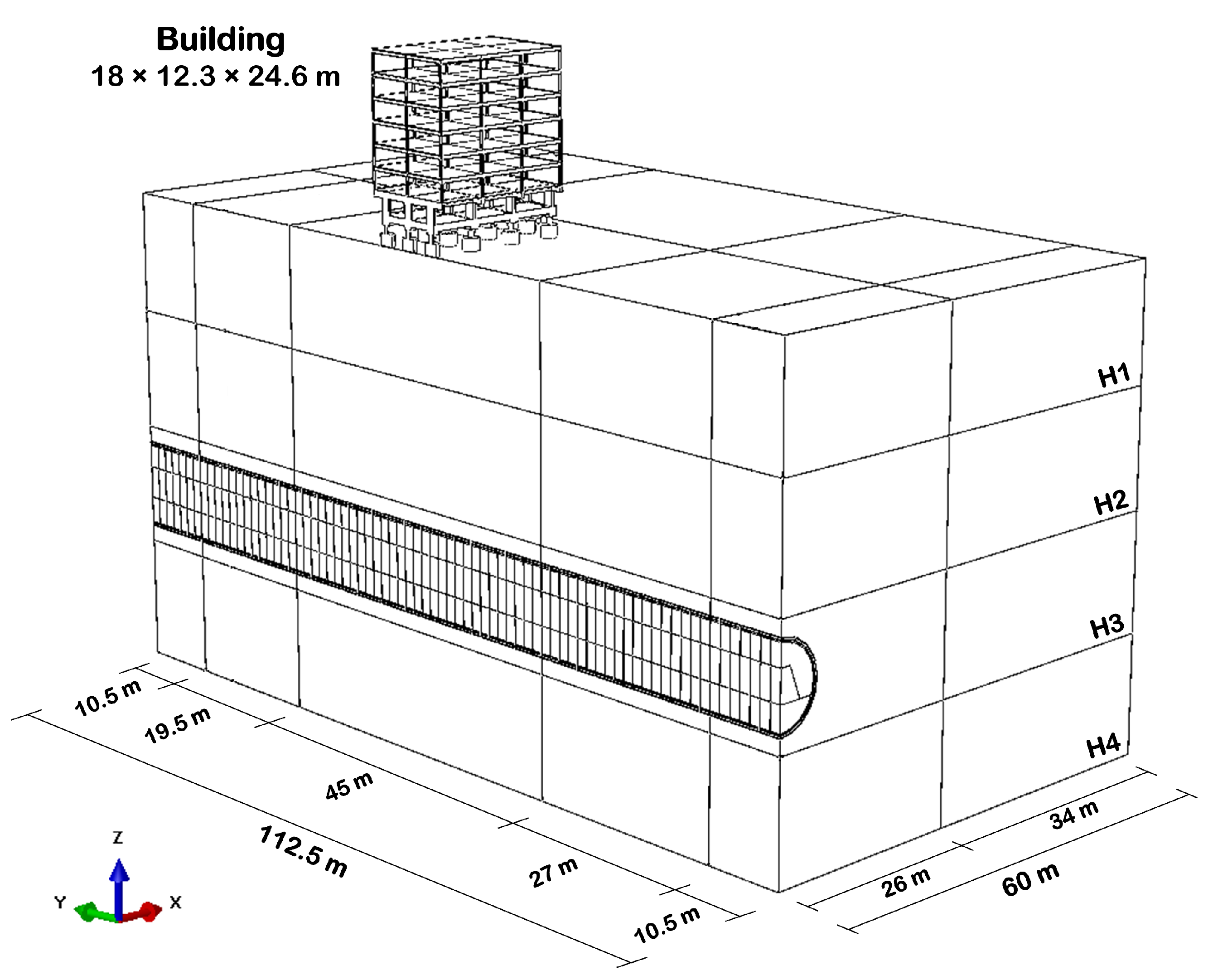
The building design was based on an expedited methodology, leading to a structure similar to other buildings constructed in Brasilia, Brazil. The details of the building, which has double symmetry, are presented in

Table 2. Summary of building structure dimensions.

Foundation
Structural Elements	Width	Length	Height	Diameter
Base	-	-	1.50	2.00
Shaft	-	-	1.00	0.60
Block	1.20	1.20	1.20	-
Beam	0.40	var.	0.80	-
Slab	var.	var.	0.10	-
First Floor
Structural Elements	Width	Length	Height	Diameter
Pillar	0.40	1.20	2.70	-
Beam	0.40	var.	0.80	-
Slab	var.	var.	0.10	-
2nd to 7th Floor
Structural Elements	Width	Length	Height	Diameter
Pillar	0.12	0.30	2.70	-
Beam	0.12	var.	0.45	-
Slab	var.	var.	0.10	-

and Figure 3.

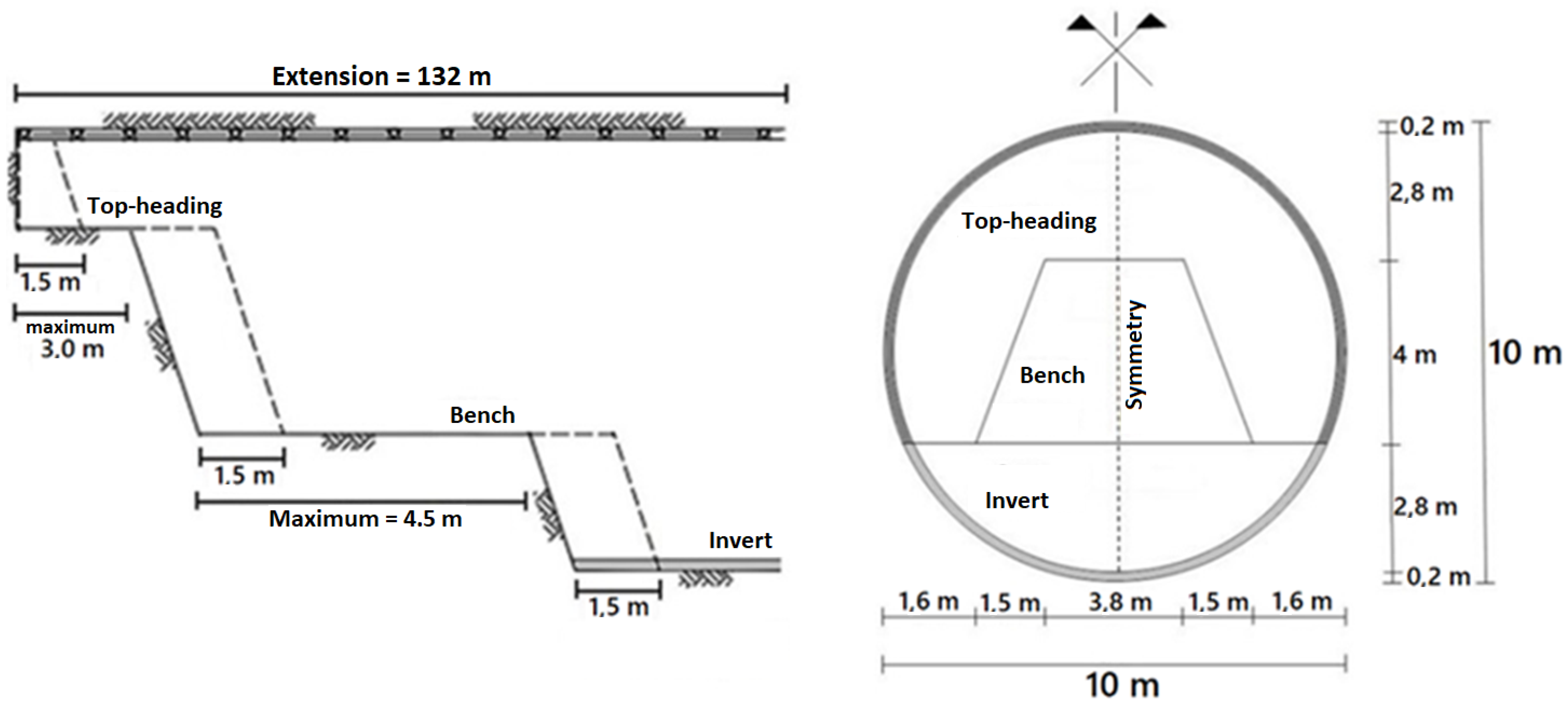
Regarding the tunnel, it has a circular cross-section of 10 m in diameter and a 0.20 m thick shotcrete support. To consider a sequential excavation, the cross-section and excavation stages were subdivided, as illustrated in Figure 4.

In the proposed methodology, the first step is to obtain a suitable deterministic model to proceed to the building of an AI surrogate model. The steps to build the FEM model are illustrated in Figure 5.

It is important to notice that the numerical model needs to be representative of the phenomenon being studied. Therefore, besides discussing the creation of the surrogate model in this research, some particularities and caveats of shallow tunnel modeling in the FEM software ABAQUS will also be explored.

4.1. Initial Model and Boundary Conditions

In the hypothetical case, the tunnel axis was considered to coincide with one of the symmetric axes of the building. The excavation began at coordinates X,Y of (0,0) and then continued until the Y = 132 m boundary condition. With this assumption, it was possible to admit a model that presents symmetry and, therefore, allows the modeling of only half of the domain. An initial design of the hypothetical case is shown in Figure 6.

In this first design, the lateral displacement boundary condition was defined at 25 times the tunnel radius. Thus, knowing that the tunnel has a radius of 5 m, this boundary condition was applied 125 m from the excavation boundary. Regarding the vertical boundaries, a rigid base was defined at a depth of 60 m, at which no displacements and rotations were allowed.

The distance from the tunnel top to the surface was 32.5 m (Figure 6), which is 3.25 times its diameter. Regarding the excavation sequence, it was initially divided into 88 steps of 1.5 m each, totaling the 132 m assigned as the y-axis domain size (Figure 4).

4.1.1. Geotechnical Parameters

Since this is a hypothetical case, the parameters were estimated within an order of magnitude considered adequate by the authors. Thus, the discussion about possible variations in the adopted values is not the main object of this study, as the parameters were not chosen to model any particular material. In this context,

Table 3. Estimated input variables.

Material/Statistical Truncated Distribution	Unit Weight (kN/m${}^3$)	Young’s Moduli (MPa)	Poisson Ratio	Friction Angle (°)	Dilatancy (°)	Cohesion (kPa)	k0
	Log-Normal	Log-Normal	Normal	Log-Normal	Log-Normal	Log-Normal	Normal
Layer H1 (0 to 15 m)	16.7–17.6	14–40	0.30–0.40	35–40	1–2	10–15	0.4–0.7
Layer H2 (15 to 30 m)	18.6–19.6	40–70	0.30–0.40	40–45	1–2	20–25	0.4–0.7
Layer H3 (30 to 45 m)	20.6–21.6	70–110	0.30–0.40	45–50	5–10	30–35	0.4–0.7
Layer H4 (45 to 60 m)	20.6–21.6	70–110	0.30–0.40	45–50	10–15	30–35	0.4–0.7
Reinforced concrete	24.5–25.5	30–32 × ${10}^3$	0.20–0.25	–	–	–	–
Shotcrete	23.5–24.5	30.5–32.5 × ${10}^3$	0.20 – 0.25	–	–	–	–

presents a summary of the input parameter ranges for all materials (Figure 6) used in the model. It is interesting to point out that it is assumed that the analysis is undertaken in the drained condition (i.e., all stiffness/strength parameters chosen are effective).

The values in Table 3 are all dimensionally consistent and ready to be inserted in ABAQUS. In addition, the authors chose to use the name of parameters that are required in that software (for example, using density and not bulk density for soils).

Regarding the distributions chosen for each parameter, the candidate families were restricted to truncated normal and log-normal distributions as these are two widely used distributions to describe geotechnical parameters [15]. To choose between these two types of distributions, both the authors’ knowledge and the study carried out by Kayzer and Gajan (2014) [15] were considered.

Table 3 presents a range of values for each random variable. As indicated, during the simulation procedure, the lower boundary and upper boundary of such intervals were used to define the smallest possible value for the parameter and the 95% percentile value, respectively. To find the actual distribution parameters (scale and location) for each RV, a system of equations obtained by locking the coefficient of variation at certain values and using the 95% percentile constraint cited previously was solved. This approach narrows the variability of the input variables to a known range and populates their domain in a way that only a few values will be sampled outside the 170 pre-sampled values. This helps to keep generalization errors controlled and almost no extrapolation is performed, as most of the time, the input variables are within a known pre-sampled range.

The coefficients of variation used were: 7.5% for the density of all materials, 10% for the Young’s modulus of concrete, 5% for the Poisson ratio of all the materials, 34% for the Young’s moduli of soils, 10% for the friction and dilation angle of soils and 40% for the cohesion of soils [14,15].

Considering that the lowest geomechanical strength parameters represent the critical condition, these were adopted in the first model of the hypothetical case to find the optimized domain and mesh. Specifically, for the Poisson ratios and k0, these values were set to 0.2 for concrete, 0.3 for soils and 0.5 for soils, respectively. Changes in the parameters were considered only after the optimized model was built.

The stratigraphic layers of the soil were considered to behave as Elastic/Mohr–Coulomb plastic materials, while the concrete was considered as a linear-elastic material.

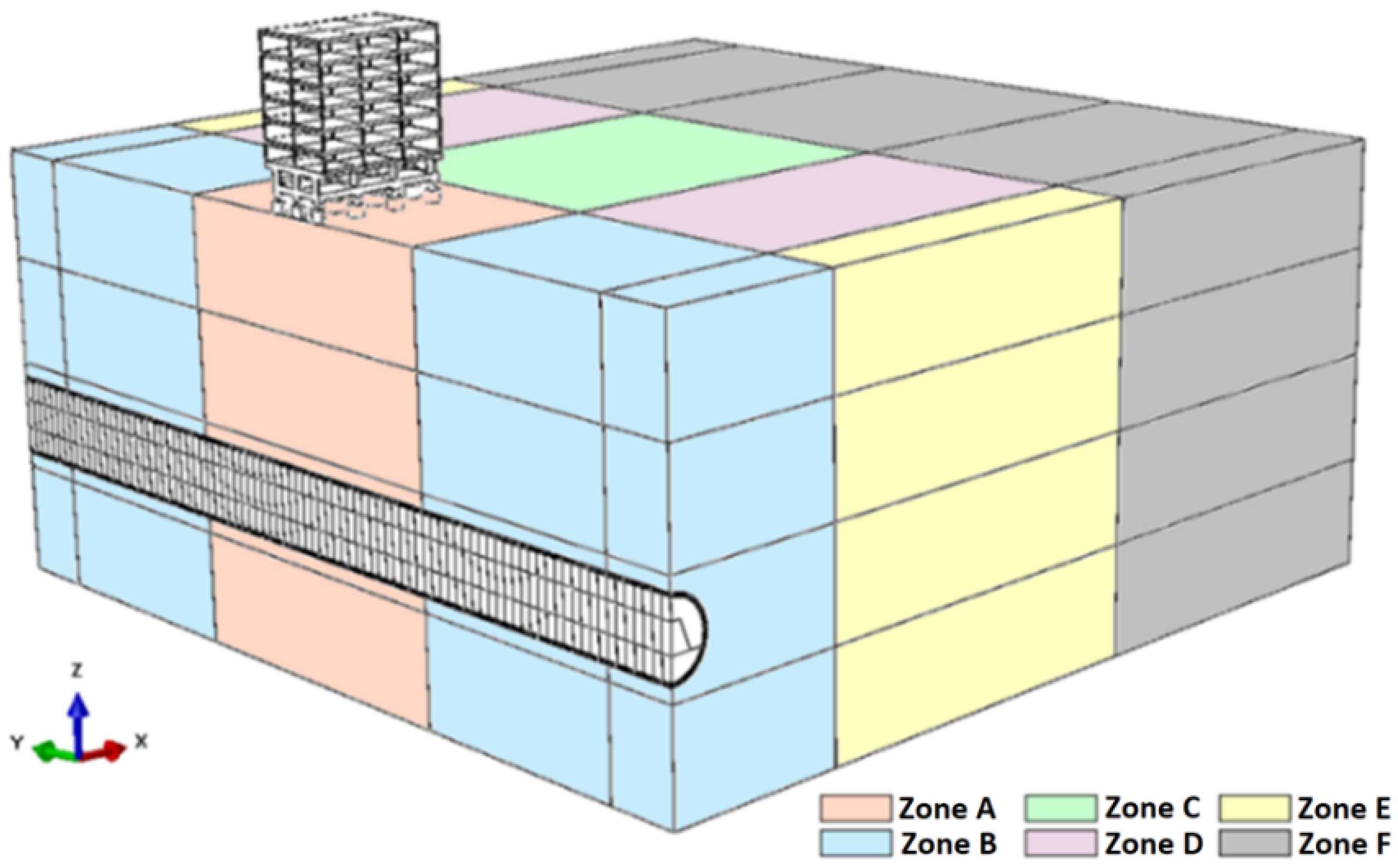
4.1.2. Mesh and Domain

The mesh was subdivided into 24 different regions to prioritize the refinement in the most important zones (Figure 7). This means that six different refinement zones were defined for each stratigraphic layer. Furthermore, the shotcrete and building structures also have particular characteristics.

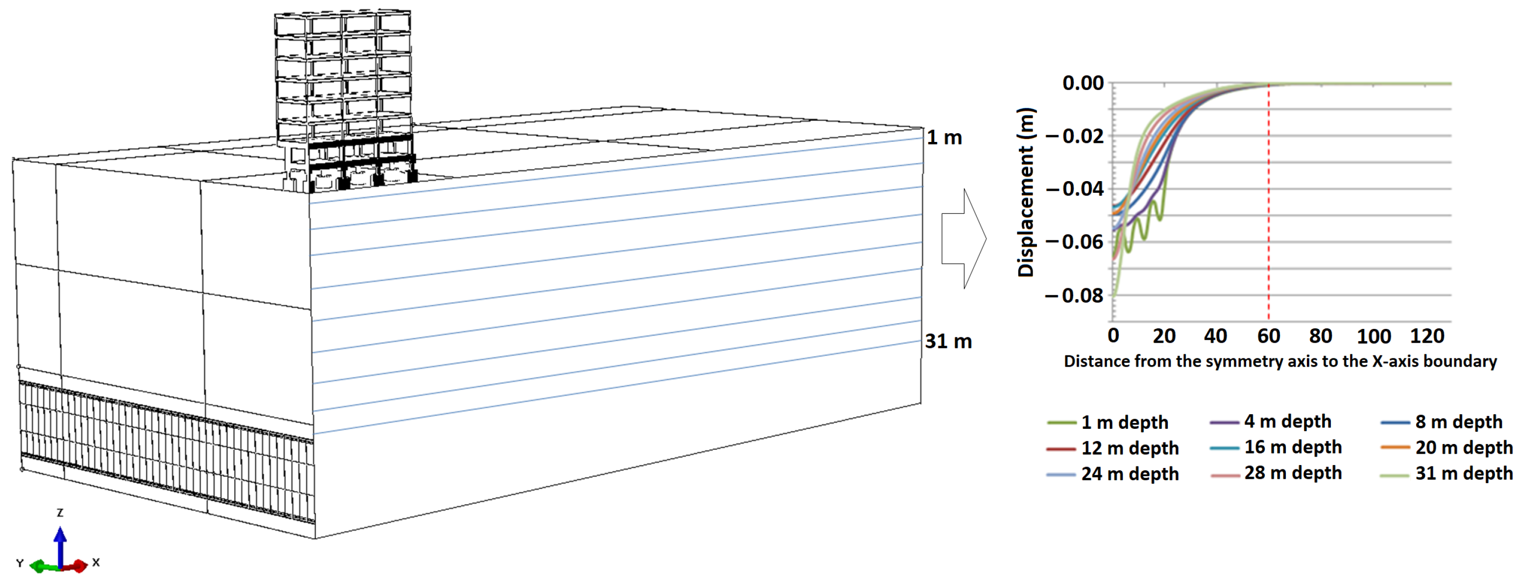
After an initial evaluation, with the mesh sizes still arbitrarily defined, the impact of the refinement in each zone was evaluated. Thus, it was possible to obtain a better cost/benefit relation involving the accuracy of the result and the processing time. For domain optimization, in the x and y axes, the sizes required to prevent boundary effects were evaluated. Regarding the z-axis, the depth indicated represents a hypothetical geotechnical constraint and, therefore, was not subject to domain optimization.

For the optimization along the x-axis, nine control paths were selected between the surface and the tunnel crown, each one with 200 points (Figure 8). The allowable tolerance to consider that the excavation front was not influencing the ground anymore was adopted as 1 mm.

The control path closest to the building foundation, with 1 m depth, was the one that had the critical convergence, in 59.15 m. Therefore, considering the most pessimistic geotechnical parameters, it was possible to reduce the size of the domain along the x-axis from 130 to 60 m. This limit was also set because at 50 m, a 2 mm influence was observed, indicating that no additional induced boundary effects would arise by setting the limit at 60 m.

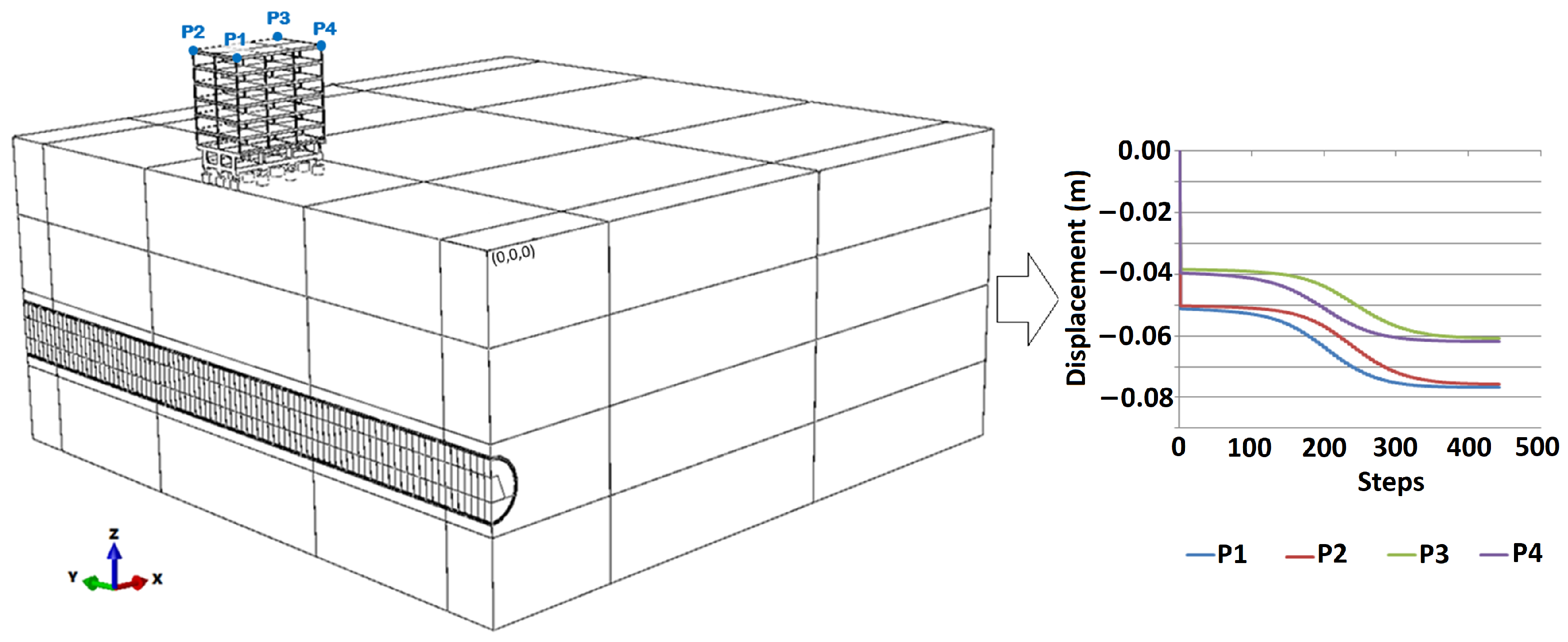
For the optimization along the y-axis, the 1 mm tolerance was also adopted. However, in this specific context, this variation was related to the advance of the excavation front and no longer the distance to the contour. This means that when the excavation induces a vertical displacement greater than or equal to 1 mm at any of the control points at the top of the building (Figure 9), the domain limit should be set to the last step of the tunnel’s invert excavation (Figure 4).

Considering the proposed methodology, it was possible to reduce the domain along the y-axis contour from 132 to 112.5 m. This reduction resulted, consequently, in a change from 443 to 378 steps. This process also considered the influence of the tunnel’s front and back boundary, discussed in more detail in Section 4.2.2.

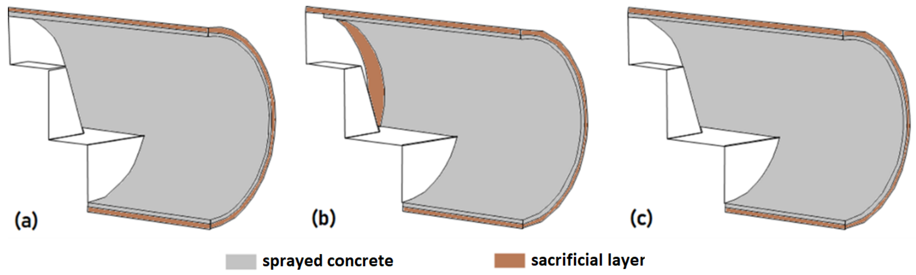
4.1.3. Contact Properties

The model was developed accounting for three distinct parts, namely: soil, building and shotcrete. To join these three different parts, the program requires a contact law to be established, which is presented in this section. Furthermore, a sacrificial layer was needed, as shall be discussed in Section 4.3.1.

As reported, there are two parts interacting with the ground that must be identified: the shotcrete and the building. For the first case, i.e., the shotcrete, a Tie contact was established, in which it is imposed that the contact surfaces should not disconnect at any time during the process. Thus, stresses and strains are transferred instantaneously between the parts.

In the interaction between the building and the top-soil layer, normal (hard) and tangential (penalty with a parameter of 0.39) behavior was established.

4.2. Optimized Numerical Model

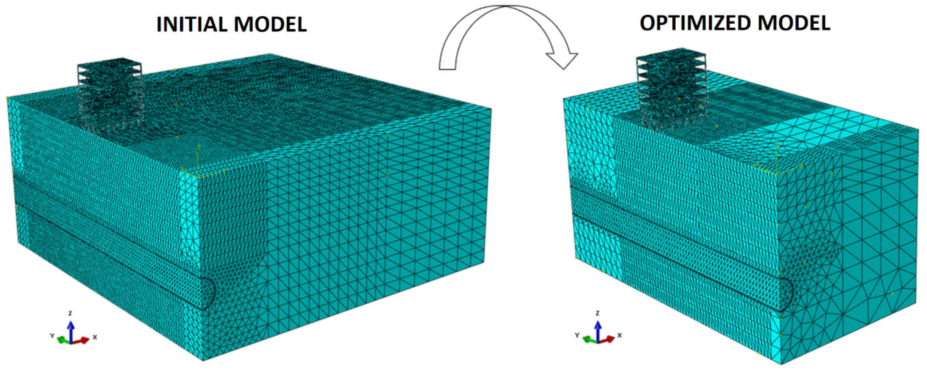
Considering the domain optimization, the model reduced the number of elements, nodes and steps, and in addition, consequently, reduced the processing time (Figure 10). Furthermore, during the model optimization, it is possible to ensure that the conditions initially proposed are adequate because there are no boundary effects and/or insufficient elements/nodes to provide the desired accuracy.

Regarding the mesh subdivision in the optimized model, it remains as shown in Figure 7, except for the exclusion of Zone F.

In order to evaluate the convergence of the mesh, besides the displacement values at points of interest, two additional indicators proposed by Raposo (2016) [53] were used. The first indicator relates the relative change of displacements between meshes with respect to the difference of the number of their nodes. The other indicates the percentage variation between the displacements obtained by different meshes. In addition, to analyze the processing time of each simulation, the same computer (CPU: AMD Ryzen 9 3950X with 128GB of RAM) was used in the refinement step, enabling a true comparison of the results.

Considering the initial model and its optimized version (Figure 11), it is possible to obtain a first visual impression of the mesh and domain optimization. It should be emphasized that 19 models were tested, with successive refinements to reach the proposed configuration. As a result, an optimized model was obtained with a 93% reduction in processing time, taking about 15 h to run. The number of elements in the optimized model is 166,670.

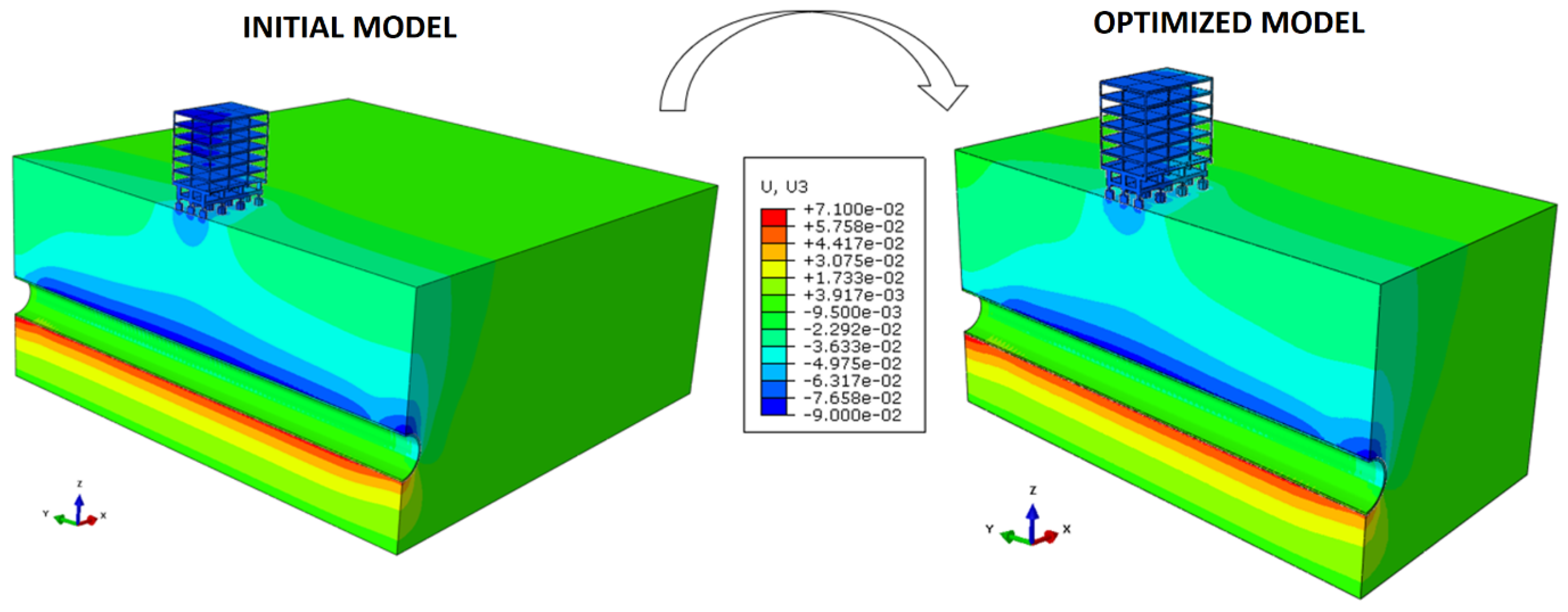
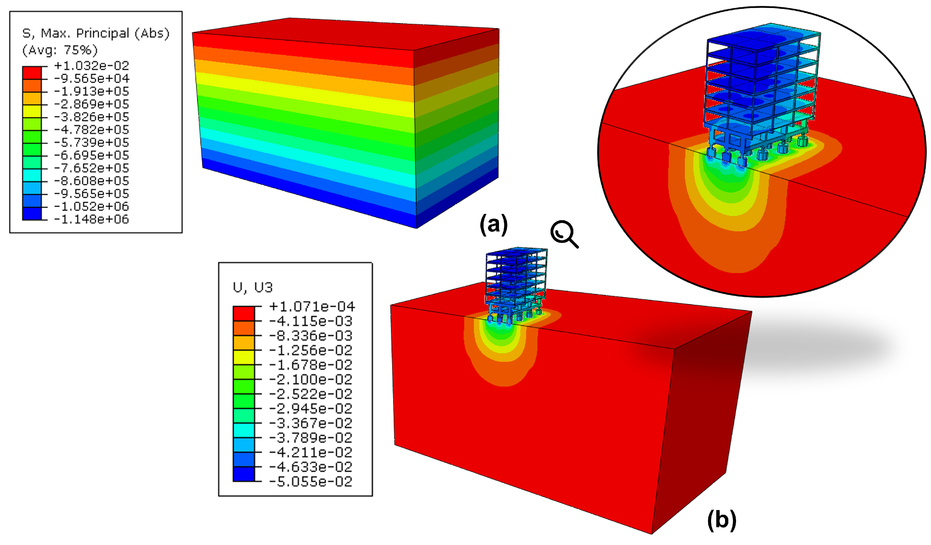
Finally, a visual way to understand the physical behavior of the hypothetical case is by displaying the vertical displacements (U3), in color scale, as illustrated in (Figure 12).

At first glance, one may see that the settlements induced by the building construction were considered in the model and that the displacements analyzed are the total accumulated values, as further explored in Section 4.2.1. It is also intuitive to see a significant influence of the tunnel excavation on the boundaries along the y-axis of the domain. For this reason, a sub-section will bring a dedicated explanation to this issue and how to isolate its effects from the simulations, including lessons learned during the process (Section 4.2.2).

4.2.1. The Building

Prior to the tunnel excavation, the model accounted for several steps, namely: equilibrium of geostatic conditions, inclusion of the building on the surface, and imposing the 1 kPa of surface loading on the slabs of each floor (Figure 13).

In this context, the analysis considers the total displacements, induced both by building construction and tunneling. This can be changed for different scenarios since ABAQUS allows discounting the influence of the construction step.

4.2.2. Tunnel’s Front and Back Boundary

The proposed tunnel has failure characteristics similar to those of a shallow tunnel. Thus, the roof yielding implies a particular characteristic for the domain’s front and back boundary while interacting with the tunnel.

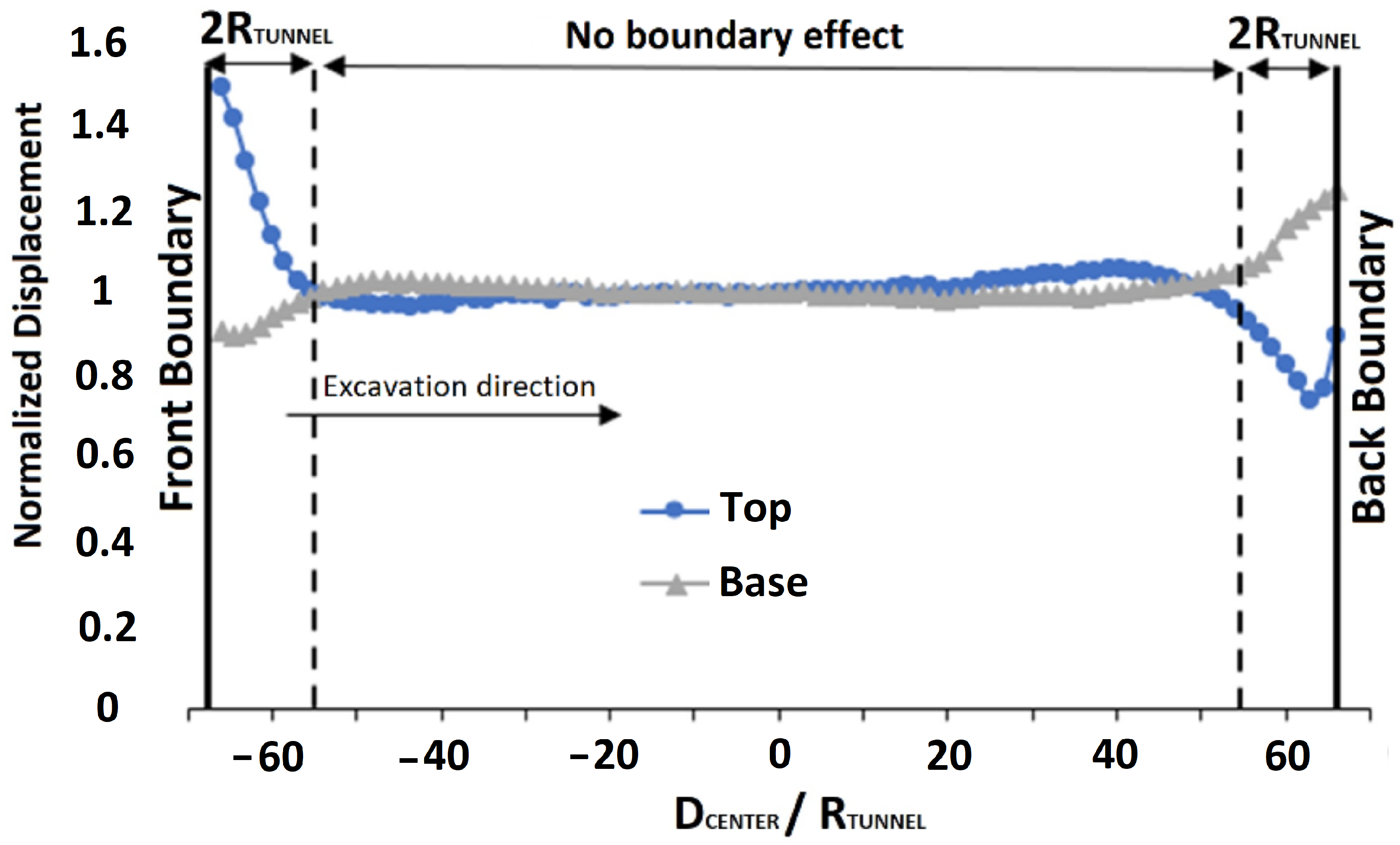
For this paper, the y-axis front and back boundary will be disregarded from the analysis in order to avoid its presence from influencing the solution. In order to make it possible, based on the experiences of Vitali et al. (2018) [54], a free field tunneling analysis was performed to verify up to which distance this influence is relevant. Thus, using control points at the top and bottom of the tunnel cross section, the displacements obtained at each excavation advance point were compared to those obtained at the mid-length of the tunnel. The result of this analysis, considering the normalized displacements, is summarized in Figure 14.

Regarding the tolerance limits, it was assigned that an acceptable deviation for the normalized displacements should be a maximum of 5%. Thus, by choosing to select multiples of the tunnel radius as the influence zone length, the interference is noticeable up to 2R.

After this analysis, it was possible to understand that the domain region at a distance of at least 2R from the boundaries along the y-axis needs to be included in the model but can be disregarded from the analysis. They need to be included to make sure the infinite tunnel scenario is observed in-between this region. Since the results will be disregarded for this region, a linear elastic model without any plasticity criterion was considered, allowing a fast calculation of the behavior of the finite elements in this region.

In the problem geometry (Figure 6 and Figure 10), it is possible to notice that this area is delimited and has an extension of 10.5 m. This approximation to 10.5 m allows the equivalence between the section and the excavation steps.

Other strategies were tested without success in this optimization process. Anyway, two attempts are worth mentioning as lessons learned from the process, these are:

• First lesson learned: the displacements and stresses were fixed as boundary conditions at the tunnel perimeter along the boundaries in the y-axis. Such stresses and displacements were exactly the ones observed at the mid-length cross-section. This attempt decreased the magnitude of the normalized displacements (Figure 14) but enlarged the affected zone, considering the 5% tolerance. Therefore, it was not useful.
• Second lesson learned: one-dimensional elements were included as reinforcement on the tunnel crown. This attempt was unsuccessful because the interference in the stress field was hardly controlled and affected even larger zones than initially foreseen.

4.3. Numerical Model Features

The present section is dedicated to discussing the numerical model features that have been developed during this work. At first, a new strategy to include the shotcrete, which required the adoption of a sacrifice layer, is described. Subsequently, simplifications adopted in solving the hypothetical case are presented.

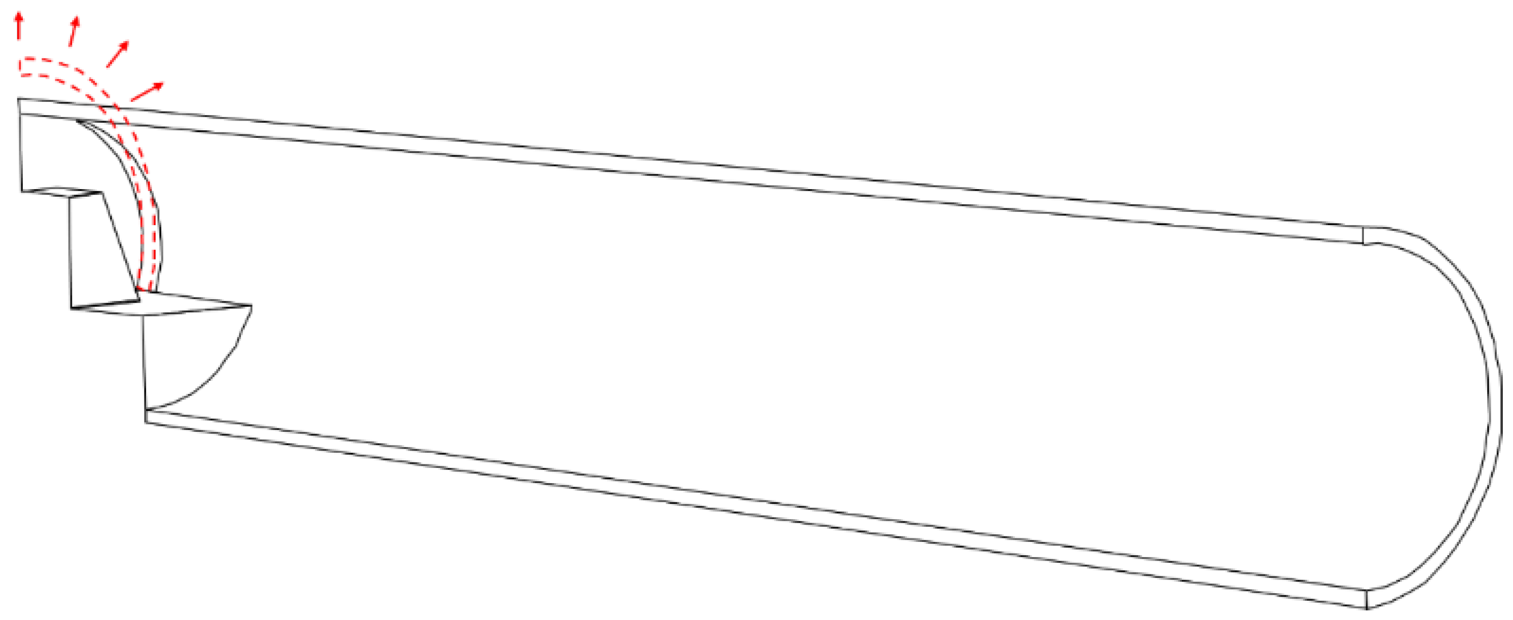
4.3.1. Strategy for Including Shotcrete

To include the shotcrete layer, ABAQUS allows both strain-free reactivation and reactivation with strain. Strain-free reactivation resets the initial configuration of the structure, while reactivation with strain does not. However, these two scenarios are not sufficient to realistically represent the tunnel behavior since shotcrete needs to be included without stresses and with a previously established diameter.

This issue comes from the fact that the original geometry (initial configuration) of the shotcrete is naturally larger (greater diameter of the cross-section) compared to the excavated section, which had already been deformed. Thus, by using the strain-free reactivation, the structure response encompasses the shotcrete pushing the soil (therefore, absorbing stresses) and reducing the previously induced displacements (Figure 15). Moreover, the final cross-section will not be executed with the designed geometric shape since the soil suffered interference in both directions.

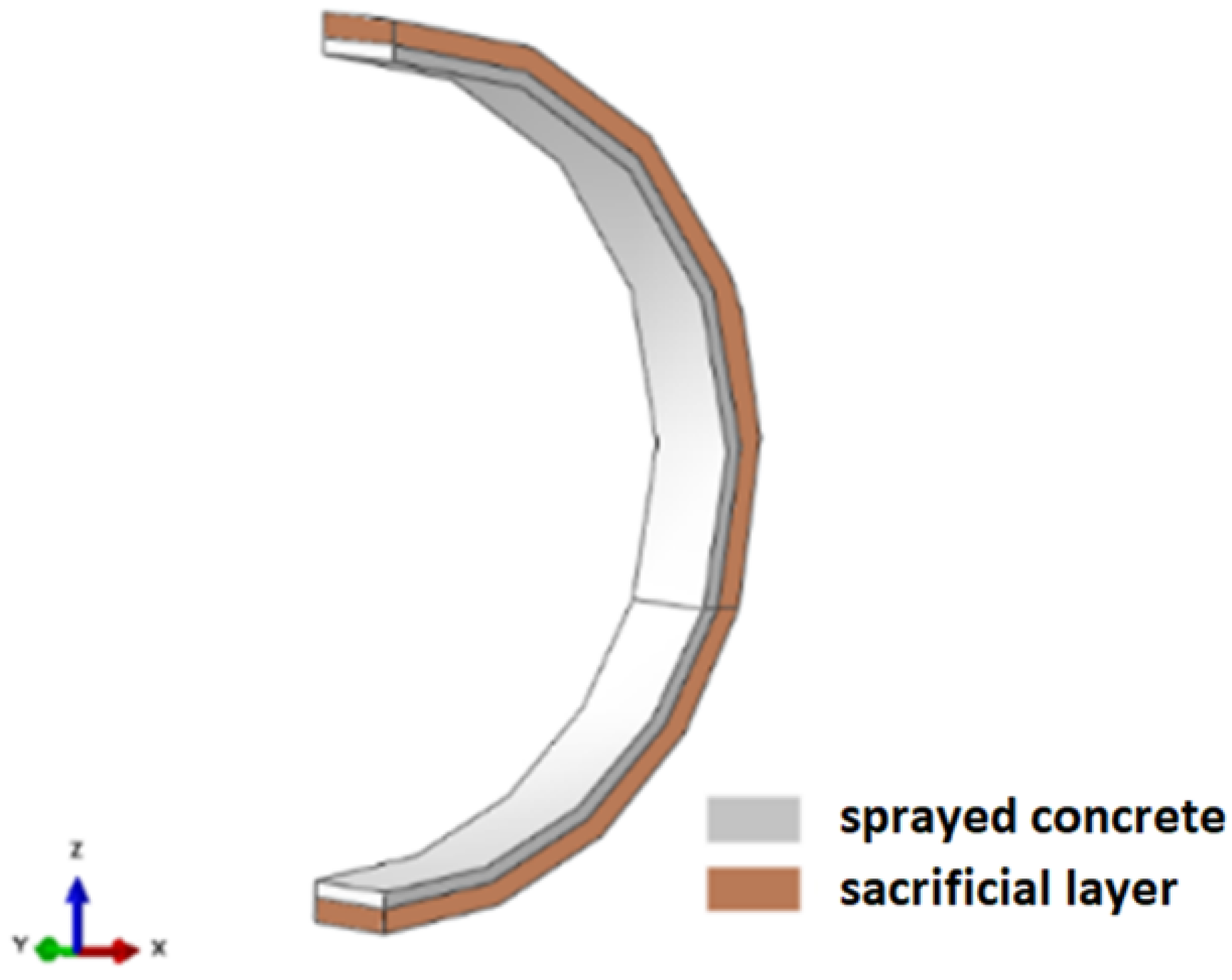
To fix this behavior, without significant interference in the model’s stresses and displacements, an extra layer was created behind the shotcrete, 0.50 m thick, named as a sacrifice layer (Figure 16).

At first, ideally a soft material should be used to model the sacrifice layer. On the other hand, the authors chose to use the same properties as the surrounding soil for two reasons. Firstly, the difference between the shotcrete’s and the soil’s Young moduli is enough to prevent most of the stress transfer. Secondly, preliminary tests made by the authors indicated that using materials that were softer than the surrounding soil started to bring excessive element deformation and distortion to the sacrifice layer, increasing the time taken for each analysis (sometimes even preventing the convergence of the algorithms). Thus, it was chosen to match the properties of the sacrifice layer to the ones of the surrounding soil.

In addition, the thickness of 0.50 m was chosen so that the volume of soil in the layer would be enough to absorb stresses and compensate for the Young’s modulus of the soil being larger than an ideal softer material. This value was defined by trial and error, checking the stress transfers to the shotcrete for several thicknesses.

The purpose of the sacrificial layer was to return the excavation to an initial geometric configuration without disregarding the effects of stresses and displacements imposed on the soil by tunneling. By introducing this intermediate layer, a large part of the local deformation energy is absorbed by the soil, diminishing considerably any stress transmission to the shotcrete as well as maintaining the geometric features of the design.

In ABAQUS, the construction methodology consisted of advancing one excavation step and allowing the soil to relax (by deactivating the inner part of the tunnel, emulating a 100% stress-relief strategy). Then, the sacrificial layer was replaced by a new one, with the same properties, attached to the shotcrete (Figure 17).

It is important to highlight that the sacrifice layer always has the same properties of the surrounding soil, even after replacing it with a new (thinner) sacrifice layer attached to a concrete (shotcrete) layer. This can be checked by analyzing Figure 16 and Figure 17. This way, the final configuration is: tunnel opening (void), shotcrete, sacrifice layer and soil massif.

It is noteworthy that the sacrificial layer is replaced only when the shotcrete is added. This layer is free to deform in the other construction stages and naturally homogenizes with the surrounding ground.

4.3.2. Simplifications Adopted

The numerical model accounts for some simplifications that may be undesirable in a practical case. However, such assumptions do not compromise the full exposition of the methodology proposed in this paper. Thus, the following points need to be highlighted:

• All stratigraphic layers were considered to be linear elastic with a Mohr–Coulomb plasticity criterion. Generally, in tunnel applications, using this constitutive model may lead to incorrect results, as it assumes the use of the same moduli to represent loadings and unloadings. Furthermore, it is also noteworthy that the linear elastic-Mohr–Coulomb model neglects other important aspects of soil behavior, such as the degradation of initial stiffness with strain, which is often important in tunnel applications [55].
• The building in the model does not include auxiliary structures such as the elevator shaft and/or stairwell;
• The building has no masonry enclosure, which may be necessary in some practical cases.

For this paper, these caveats are known, and nevertheless, it was chosen to adopt them in exchange for a lower computational time. The probability of failure calculation methodology is not affected by these facts, and, in a practical case, other approaches may be desirable.

5. Results and Analyses

In general, as the FEM model was built, one has to obtain 170 (about 12 times the number of independent input variables or 5 times the number of dependent input parameters) deterministic solutions of the numerical model, considering the variation of the 34 input parameters proposed for the hypothetical case. Each model runs for about 15 h, leading to a total of 2550 h (about 106 days) of simulations in a powerful workstation. Such long simulation times put into context the need for AI approaches and why the probability of failure cannot be computed (or validated) using simple Monte Carlo simulation with the FE model.

Then, the application of 31 different artificial intelligence techniques is performed to check the relative importance of the 34 input parameters to the output result, which was chosen to be the vertical displacement at the bottom of each foundation element. An RFECV algorithm was applied to find the most important input parameters with respect to the output chosen (vertical displacement at the bottom of foundation elements). After selecting the input RVs, several techniques were used as regressors, where about 75% of the samples (128 out of 170) are applied for training and another 25% (42 out of 170) for testing and verifying accuracy. Subsequently, in the fourth methodological step, it is possible to interpolate the 170 results with acceptable precision, and thus achieve ${10}^7$ result samples in a short time. Finally, it becomes feasible to verify the reliability of different sampling techniques in an acceptable amount of time.

As indicated, the focus will be on the vertical displacements (U3) at the bottom of each foundation element. Thus, knowing the coordinate system of the global problem (Figure 10), it is possible to identify the foundation elements in Figure 18.

For each of the footings, a control point was assigned at the central node of the respective foundation element. Thus, the surrounding elements of each footing were represented in

Table 4. Influence between footings.

Footing	Influence Zone	Footing	Influence Zone	Footing	Influence Zone	Footing	Influence Zone
A	D-B	D	A-G-E	G	D-J-H	J	G-K
B	A-E-C	E	B-D-H-F	H	E-G-K-I	K	H-J-L
C	B-F	F	C-E-I	I	F-H-L	L	I-K

.

For the methodological validation, the present study is limited to investigating the relationship between footings A and D. The choice for this pair is justified by the criticality of the displacements in this region.

5.1. Variable Sensitivity Analysis

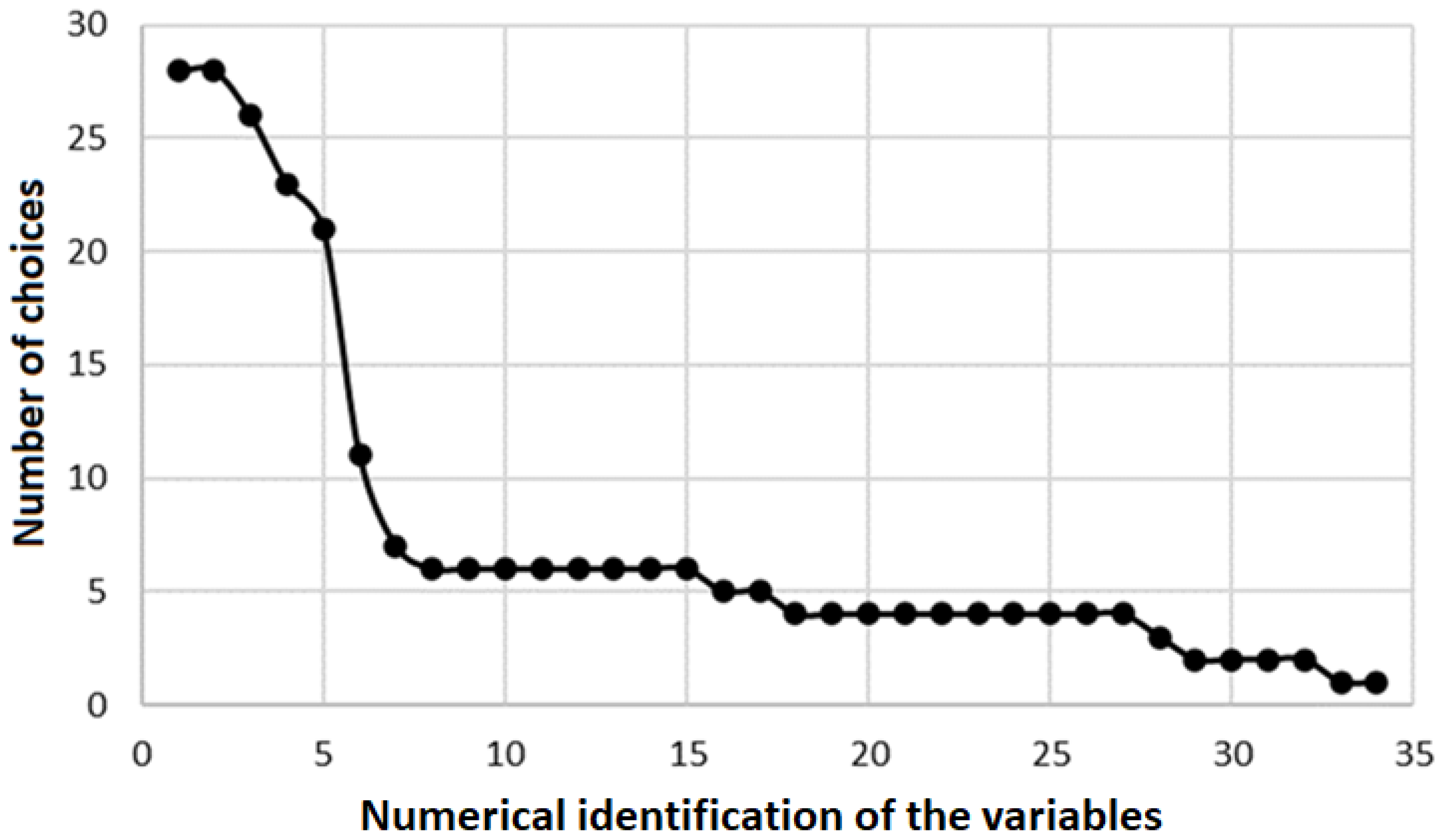
The sensitivity analysis of the random variables was based on the influence that the parameters have on the vertical displacement (U3) of the footings, according to the methodology detailed in Section 3.2. To evaluate the results, it was plotted how many times each of the 34 random variables was identified as relevant by the 31 different artificial intelligence techniques that were tested in the scope of the Python® RFECV package (Figure 19).

It can be seen in Figure 19 that between the fifth and the sixth variable, there is a significant gap. Considering this result, only the first five random variables should be considered.

Table 5. Relative importance of each parameter.

Parameter	Number	Global Importance 1	Local Importance 2
	of Choices	(%)	(%)
Layer 1—Young’s Modulus	28	75.4	78.0
Layer 3—Young’s Modulus	28	7.4	11.2
Layer 3—k0	26	2.7	5.7
Layer 1—Poisson	23	1.0	3.0
Layer 2—Young’s Modulus	21	0.6	2.1
∑		87.1	100.0

shows details of the variables chosen and their importance percentage to predict the vertical displacement of Footings A and D.

By restricting the input parameters to those presented in Table 5, the best scoring AI technique among the 31 tested was the ExtraTreesRegressor. This way, a closer look at the learning process of this specific algorithm is presented in the next section.

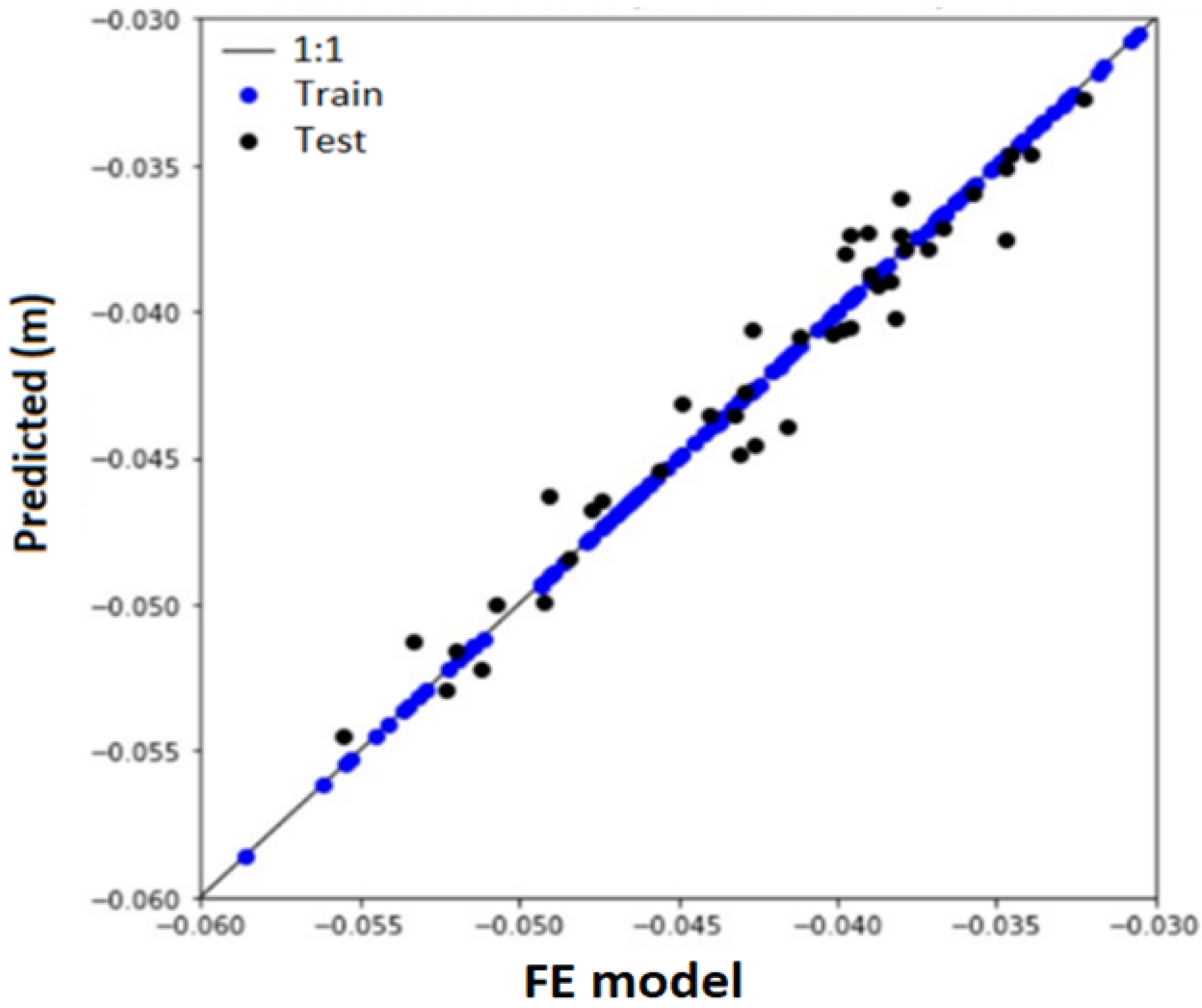
5.2. Training and Testing the Artificial Intelligence

To adjust the decision tree, which used the technique named ExtraTreesRegressor, about 75% of the sample (128 out of 170) was used for training and 25% (42 out of 170) for testing, according to the methodology detailed in Section 3.3. Without further hyperparameter tuning, this method was able to represent a surrogate model for the FEM numerical modeling with accuracy higher than 95% for both footings A and D. The parameters used during the fitting procedure were: ‘bootstrap’: False, ‘ccp_alpha’: 0.0, ‘criterion’: ‘mse’, ‘max_depth’: None, ‘max_features’: ‘auto’, ‘max_leaf_nodes’: None, ‘max_samples’: None, ‘min_impurity_decrease’: 0.0, ‘min_impurity_split’: None, ‘min_samples_leaf’: 1, ‘min_samples_split’: 2, ‘min_weight_fraction_leaf’: 0.0, ‘n_estimators’: 100, ‘n_jobs’: None, ‘oob_score’: False, ‘random_state’: 42, ‘verbose’: 0 and ‘warm_start’: False. A full description of each parameter’s behavior and effect can be found in [56].

Regarding Footing A, the accuracy obtained was 97.61%, a mean absolute error of 1 mm, and a maximum absolute error of 2.8 mm. Figure 20 illustrates the results obtained in the training stages and the predictions for the tests performed. Since we reached a tolerable mean absolute error of about 1 mm, no further parameter optimization was performed.

For Footing D, the accuracy obtained was 97.57%, a mean absolute error of 1 mm, and a maximum absolute error of 2.7 mm. Figure 21 illustrates the results obtained in the training stages and the predictions for the tests performed. Since we reached a tolerable mean absolute error of about 1 mm, no further parameter optimization was performed.

5.3. Reliability of Sampling Techniques

The reliability of the LHS technique was obtained by comparing its results with those predicted by simple Monte Carlo sampling, according to the methodology detailed in this section.

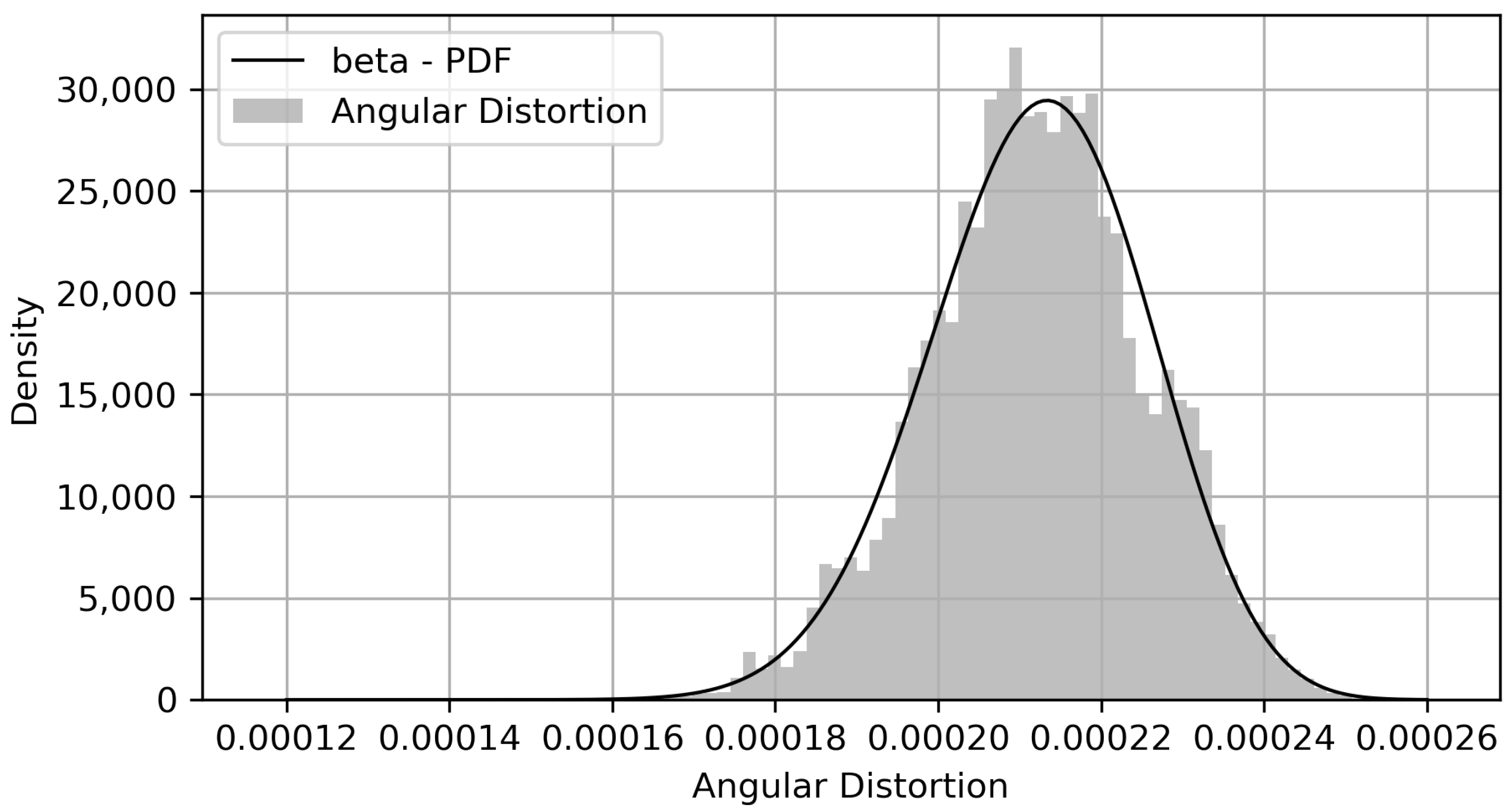
Note that the sampled data were fitted to a Beta distribution [57], which was found to be the third-best distribution in accordance with the AIC criterion. Still, the squared error of the first two distributions indicated a poor fit. The top five distributions are presented in

Table 6. RV ranking.

Parameter	AIC	Squared Error
Von Mises (vonmises)	−$1.50891\times {10}^8$	$6.82\times {10}^{67}$
Gauss hypergeometric (gausshyper)	$-2.72042\times {10}^7$	$3.29\times {10}^{13}$
Beta (beta)	$-1.96046\times {10}^7$	$2.07\times {10}^8$
Johnson SB (johnsonsb)	$-1.96045\times {10}^7$	$2.06\times {10}^8$
Pearson type III (pearson3)	$-1.96042\times {10}^7$	$2.02\times {10}^8$

.

The visual agreement between the empirical histogram and the fitted distribution is presented in Figure 22.

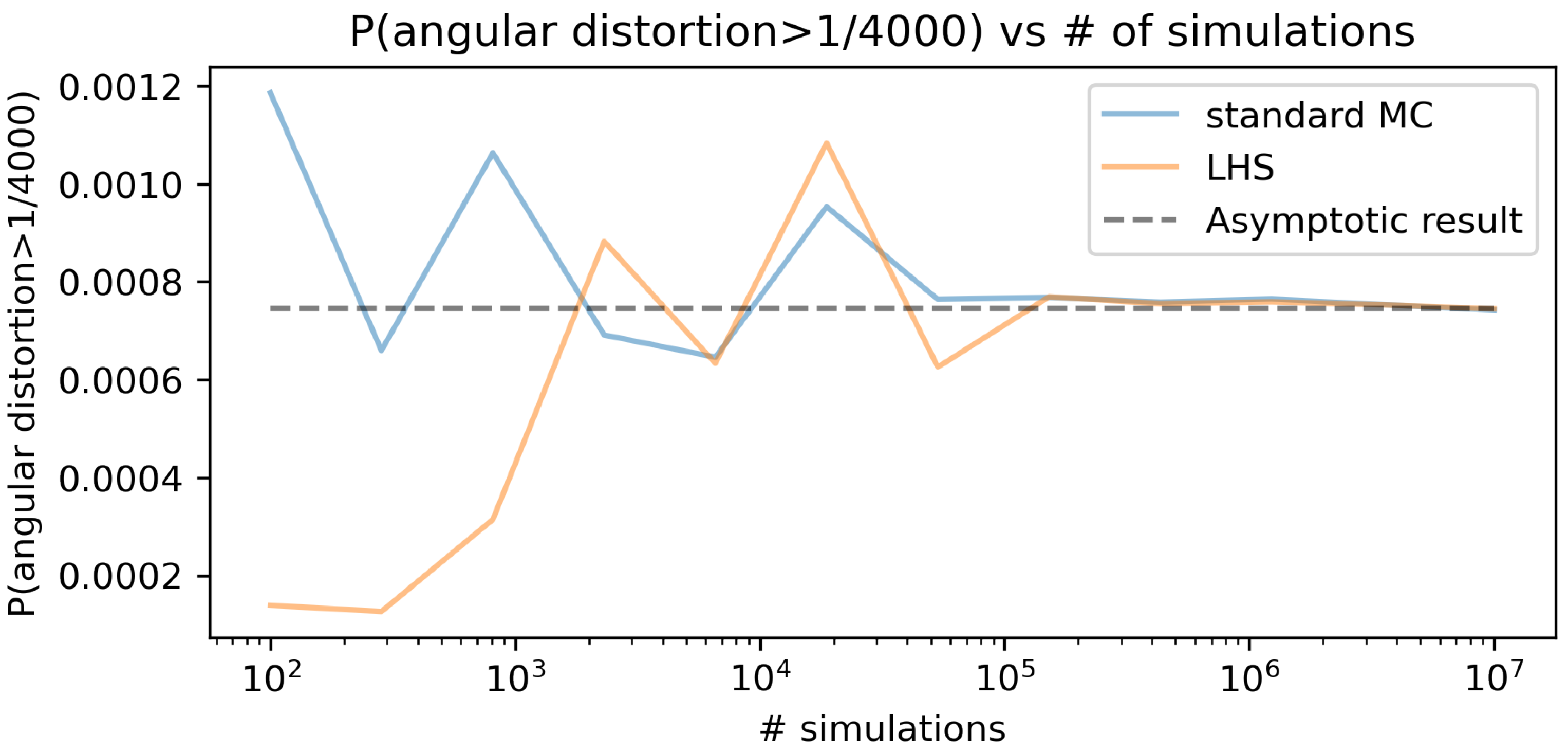
Considering the results obtained in the hypothetical case, the probability of failure was analyzed as the probability that the angular distortion is greater than 1/4000 ($2.5\times {10}^{-4}$), hereby defined as the SLS criterion. Furthermore, this was the value chosen as the reference to plot the convergence graph of the techniques studied (Figure 23). Although values lower than this reference cannot be associated with failure in the Serviceability Limit State—SLS, as Table 1 suggests, the exercise validates the methodological procedure. In other words, this value was chosen to produce small, but tractable, probabilities of failure. Comparing the convergences of Latin Hypercube Sampling (LHS) and Simple Monte Carlo Sampling (MC), considering the 12 points analyzed, the results are presented in Figure 23.

As indicated, the “true” value of probability of failure is chosen as the asymptotic probability of failure for the Monte Carlo simulation ($p_f$ = 0.00074248). If one allows up to 2% difference to the true result (asymptotic result), the LHS calculated probabilities stay within this band (from 0.98 $p_f$ to 1.02 $p_f$) for 432,876 samples (for which the calculated probability is of 0.00075514) onward. On the other hand, for the standard MC sampling method, the calculated failure probabilities only stay within the 2% band from 3,511,191 samples (probability of 0.00075294) onward. This reveals that 12.3% of the number of samples of the MC were needed for the LHS to be within a 2% error band. This result is exploratory, and further validations are needed to perform a full comparison between intelligent sampling techniques and standard MC. On the other hand, it suffices to illustrate the process of obtaining a surrogate AI model and sampling it a large number of times (in this scenario, ${10}^7$ samples could be obtained in 57 s for standard MC).

6. Conclusions

Artificial intelligence techniques are promising tools for risk analysis. Concerning the calculation of the probability of failure in urban tunnels, it is common to build complex numerical models that require high computational power. Thus, in order not to be limited to a deterministic approach, the interpolation of results by artificial intelligence techniques proves to be adequate. This process of creating a surrogate model by using AI is novel in the shallow tunnel modeling scenario, which indicates the importance of this work.

The Latin hypercube sampling technique has shown promising results both as a space-filling technique as well as a fast-converging sampling scheme. Using this technique, it is possible to reduce the number of samples collected in the numerical models without losing the desired accuracy. Limited to the results of the study case carried out, it is noteworthy that the LHS was able to achieve results within 2% of error from the “true” asymptotic value with only about 12% of the sample size needed for the standard MC sampling technique.

The methodological application in the hypothetical case proved to be adequate for the validation of the concepts. The combination of numerical analysis, artificial intelligence techniques and intelligent sampling algorithms showed to be a promising method capable of being adapted to real practical cases.