1. Introduction
Railway transportation is a significant mode of transportation for reasons of environmental friendliness, safety, cost, and lower energy consumptions. It is a sustainable mode of transportation that supports the economic and industrial expansion of the society through the mobilization of freight and passengers [
1]. The growing demand to shift huge volumes of passengers and freight traffic and the current state of the existing railway infrastructure are issues that require substantial attention in the field of transportation [
2]. Capital expansion of the railway infrastructure is a cost-intensive and time-consuming approach. Thus, the maintenance and renewal (M&R) process needs to be subjected to continuous improvement for the existing infrastructure to meet the capacity demand without compromising the quality of the provided service [
3,
4].
The operational capacity of a given railway infrastructure is significantly influenced by its utilization methods and its technical state or quality [
5]. One of the key aspects of railway infrastructure maintenance is the inter-dependability of its operational capacity and the infrastructure condition. A high operational capacity with good service quality is achieved when the infrastructure is in a good state with high quality. With the increase in capacity utilization, the infrastructure is subjected to a higher traffic load leading to rapid deterioration of the infrastructure and degradation to its components. This consequently leads to higher M&R needs which require track possession, and thus eventually resulting in the reduction in operational capacity. The downtime arising from these M&R of networks is responsible for nearly half of all the delays to passengers. In Sweden, an average of 572.7 h per year of delay is incurred due to the failure of components in the railway track [
6]. To mitigate such delays and to ensure safe, sustainable, and reliable operation, the track and its components need to be inspected frequently.
Rail fastening systems are a vital component in the railway track system as they clamp the rail to the sleepers, preventing the longitudinal, transverse, and lateral deviation of the rail from the sleepers, thus aiding in preserving the designed track geometry. Failures of fasteners can also widen the gauge, increase wheel flange wear, reduce the safety of train operations, and may lead to catastrophic accidents [
7]. At present, the inspection of track fasteners is carried out by manual inspection or using track inspection cars. Manual inspections are slow, labor-intensive, pose safety issues for maintenance staff, and are prone to human errors. Manual inspections are furthermore time-consuming and expensive for railroad companies, especially for long-term and large-scale development projects. Fastener inspection based on inspection cars has limited capabilities when it comes to inspection frequencies and requires track possession during the inspection process, thus reducing the operational capacity [
8]. With the continuous expansion of the railway network and recent technological developments, an automated rail inspection system based on machine vision has gained significant importance. To inspect track defects and detect the presence/absence of the fastening bolts, References [
9,
10] introduced their vision system for real-time infrastructure inspection (VISyR) system, which was a fully automatic and configurable field programmable gate-array (FPGA)-based vision system for real-time infrastructure inspection. The system used a Dalsa Piranha 2 line camera (Matrox) with 1024 resolution to acquire images of the rail. An image-based detection device comprising of two industrial laser range scanners, one for each rail, was used by Babenko [
11] to inspect fasteners. On the acquired images, a convolutional filter bank was applied in this study. Each fastener type had a filter associated with it and the coefficients for each were estimated using an illumination normalized version of the Optimal Trade-off Maximum Average Correlation Height (OT-MACH) filter. A track cart was used by Resendiz et al. [
12] to capture the video of the railroad track with off-the-shelf cameras. A texture classification with a bank of Gabor filters followed by support vector machine (SVM) was used to determine the location of the rail components from the captured video. Structured light sensors were employed by Mao et al. [
13] to inspect fastener conditions and they used a decision tree classifier to classify the defects in the fastening system.
The application of automated machine vision for fastener inspection has predominated over the past two decades, but the detection methods from these images have varied over time. Image processing and deep learning-based methods are the two commonly employed methods for detecting fasteners from the images [
8]. Locating and segmenting the fastener region, extracting fastener features, and using a classification algorithm for fastener defect identification are the three main aspects of the image processing-based method. For detecting missing hexagonal-headed bolts, Marino et al. [
9] made use of a multilayer perceptron neuron classifier. Stella et al. [
14] employed principal component analysis and wavelet transform for pre-processing the fastener images and used a neural network classifier to detect missing hook-shaped fasteners. To match the fastener images, Yang et al. [
15] used direction field as a template and used linear discriminant analysis (LDA) for matching and to obtain the weight coefficient matrix. Ruvo et al. [
10] adopted an error backpropagation algorithm on the rail images to model two types of fasteners and introduced a FPGA-based architecture [
16] using the same algorithm. AdaBoost [
17,
18], structure topic model (STM) [
19], line local binary pattern (LLBP) [
20], support vector machines (SVM) [
21], and edge detection methods [
22] are other frequently used techniques to detect fasteners from rail images. These traditional methods aid in fastener inspection with minimal manpower and reduced equipment resources; however, the detection accuracy could easily stagnate as it is difficult to manually design robust and accurate features for rail components due to the diversity of shapes and complex backgrounds [
23]. With the increase in computing power and development of the graphical processing unit (GPU), deep learning methods [
24,
25,
26,
27,
28] for detecting fasteners from rail images have gained substantial importance.
Over the past few years, significant advancements have been made in detecting fasteners and identifying the defects from railway track images; however, there are some underlying drawbacks associated with this method. The robustness and position accuracy are two major concerns associated with this mode of fastener detection [
26]. It is a relatively expensive task to mount and maintain a reliable and high-quality automated visual inspection system as they are integrated with the operation and are subjected to vibrations, brightness fluctuations, and motion blurring during high-speed travel. This can deteriorate the accuracy of fastener condition detection and can raise safety concerns. Furthermore, the detection task becomes complicated when rail and its components are concealed due to the presence of rust and dust. Another significant drawback of this method is its inability to detect the rail and its components when they are obscured due to the presence of snow, sand, stones, and other debris. This calls for a removal process or additional rail surface treatments that add to the expense of the railroad companies. In Sweden, around 298,080 EUR were spent in 2014 to inspect two lines with a track length of ca. 300 km, of which more than 75% was utilized to inspect track components that exhibit magnetic characteristics (rail fastening, weld joints, insulation joints, etc.) [
29]. With the extension of high-speed railway networks, the maintenance managers are striving to reduce these operation and maintenance costs through effective condition-based maintenance (CBM), while augmenting the quality and capacity of the rail services.
Non-destructive testing (NDT) plays a significant part in the condition-based maintenance of railway infrastructure. Eddy current (EC) testing is one of several NDT methods that work on the principle of electromagnetism, which is used for examining metallic components. In earlier research, the authors proposed a train-based differential eddy current sensor [
6,
29] for fastener inspection that can overcome the major challenges associated with the visual inspection. EC sensors work on the principle of electromagnetism and are not affected by the presence of nonconductive materials in the sensor-to-target gap. EC sensors can be used in dirty environments, such as water, oil, etc., where other inspection system fails. The proposed inspection technique using differential eddy current sensors was able to detect fastener signature when mounted on a trolley system at a distance of 65 mm above the railhead. The results presented in the previous literature were based on controlled measurements carried out on multiple short track sections, where the likelihood of disturbances was minimal. The missing clamp detection model in the previous study made use of supervised machine learning models with data points that had predefined labels to train the model and optimize their label recognition capacity in a given data set. The present study reports a case study where the measurement system was mounted on an in-service freight train and where the fastener condition and other likelihood of disturbances were unknown. This case study aims to implement unsupervised anomaly detection to the measurements obtained from a train-based differential eddy current sensor for monitoring railway fastening systems. The purpose of this study was to facilitate the development of a train-based automated measurement system for inspecting railway fastening systems and detect and analyze anomalies from the fastener inspection measurement.
The remainder of this paper is structured as follows.
Section 2 elaborates the research methodology followed for this case study. The results and analysis from the study are explained in
Section 3 and the conclusions and future work are discussed in
Section 4.
2. Methodology
The proposed unsupervised fastener detection models are based on applying algorithms capable of recognizing patterns and relationships in the data, without any prior knowledge. The devised detection model will make use of two unsupervised machine learning models. The first model is implemented for detecting anomalous behavior from the given data points to separate the healthy class from the anomalous class. The next model will make use of a clustering technique on the data points to segregate them into different groups to extract meaningful information regarding the anomalous points.
2.1. Data Collection
2.1.1. Differential Eddy Current Sensor—Lindometer
For decades, the eddy current method has been well known for the non-destructive testing of electrically conductive objects [
30]. EC testing is based on the phenomenon of electromagnetic induction, where an alternating current passing through a conducting coil creates an oscillating magnetic field. Every coil is characterized by an impedance (
, which is a complex-valued generalization of resistance, for a single frequency sinusoidal excitation
f. The impedance of the coil (refer Equation (1)) [
31] can be expressed as:
where
and
are the voltage and current across the coil and
is the resistance and
is inductive reactance of the coil with an inductance of
. Impedance
has a magnitude
and phase
φ [
31] (refer Equations (2) and (3)).
EC inspections are based on Faraday’s law of electromagnetic induction which states that a circular current is induced in an electric conductor due to an alternating magnetic induction flux. In turn, the induced circular current, known as the eddy current, creates a secondary magnetic field that tends to weaken the effect of the primary magnetic field. As the EC intensity increases in the test piece, the imaginary part of the coil impedance decreases. The real part of the coil impedance also reduces as the EC contributes to the increase in power dissipation of energy. The new coil impedance (
(refer Equation (4)) [
31] can be expressed as:
EC inspection generally measures this change in coil impedance from
to
in the form of either current or voltage signals to extract information of the test piece. EC density is greatest on the surface and is not uniformly distributed throughout the entire volume of the test piece. The current flow decreases exponentially as the distance from the surface of the test piece increases. The skin depth (refer Equation (5)) [
31] (
δ) is the distance from the surface at which the eddy current density decreases to a level of ‘1/
e’ of its surface value and is expressed as:
where
is the conductivity given by the reciprocal of resistivity (
ρ)
σ = 1/
ρ,
µ is the magnetic permeability, ω is the angular frequency of the current given by
ω = 2π
f.
In principle, eddy current sensors are sensitive to local fluctuations of the magnetic permeability (
µ), conductivity (
σ), and the geometric form of the material, and hence can be used to detect inhomogeneities along the rail track [
30]. For train-based applications, differential EC sensors are preferred. The differential EC sensor used for this case study was developed by Alstom Transport (Stockholm, Sweden) and was named as ‘Lindometer’.
Figure 1 depicts the proposed sensor consisting of one driver coil ‘D’ and two pick-up coils ‘P1′ and ‘P2′. The driving coil ‘D’ is driven by a sinusoidal primary current
i(
t) that generates an alternating primary magnetic field. Eddy currents are thus induced within the rail and other electrically conductive components located in the proximity of the sensor. As a result of these ECs, a secondary magnetic field is generated, which has an opposite direction to that of the primary field, complying with Lenz’s law.
The information along the rail is represented as variations in amplitude or phase or a combination of both, which are extracted and analyzed using demodulation techniques. The size of the driving coil is approximately 18 (z), 70 (x), and 155 (y) mm. The two pick-up coils are encased by the driving coil which acts as an outer winding. The winding is applied in one layer with 22 turns using a copper wire of 0.7 mm diameter. The pick-up coils have a size of 18 (z), 30 (x), and 150 (y) mm, with each coil having a winding applied in one layer with 94 turn with a copper wire of diameter of 0.16 mm. The two pick-up coils are placed side by side along the x-direction with a gap of 4 mm.
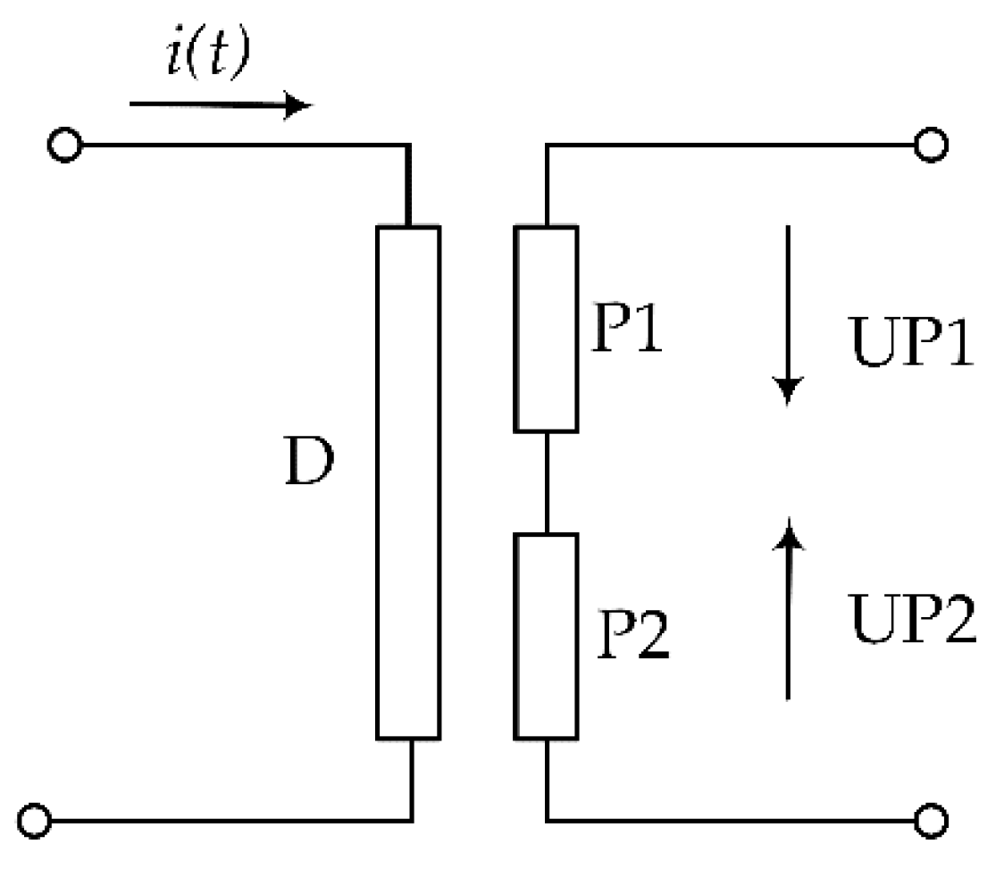
The two pick-up coils are enclosed by the driving coil and differentially coupled as depicted in the circuit diagram given in
Figure 2. The differentially coupled pick-up coils cancel out the cross talk between the pickup and driver coil, though not completely. The resulting voltage
u(
t) is the result of the induction of the ECs along the rail and the cross talk residue that are linearly superimposed. The quality of the cross talk cancellation is determined by the geometrical symmetry between the three coils, and hence the windings are placed in an even layer with no crossovers. EC is generated in the rail and vicinity along the
x-
y plane by the driving coil and the pick-up coils are sensitive only to the
z-component of the generated flux due to the geometrical orientation, as depicted in
Figure 1. The differentially coupled pick-up coils (P1–P2) are sensitive only to the changes in the EC along the rail and its vicinity. If there is an even surface (as an ideal rail with no other electrical components or defects) with no change in the geometric form of the material, or conductivity (
σ) or magnetic permeability (
µ), the resulting voltage will be zero due to the induction of similar ECs all across the place. When there is a change in the geometry or conductivity of magnetic permeability at one single point along the rail and its vicinity, a change in EC takes place. Only the singular point with the EC change will create a signal, due to the symmetry of the differentially coupled pick up coils, given by (refer Equation (6)).
The Lindometer encloses two such independent differential EC sensors placed at a distance of 20 cm apart. The Lindometer uses two driving fields at frequencies of 18 and 27 kHz, respectively. Two channels were installed within the Lindometer to facilitate future speed measurements using cross-correlation techniques. The above-mentioned frequencies fall under the rail norms and can be used for inspecting track and its components. For this case study, only one channel with the driving field of frequency 27 kHz was used for the measurement along the track. To stabilize the sensor, both against temperature drift and vibration, the entire unit is vacuum potted with epoxy resin.
2.1.2. Case Study: Train Measurement along the Iron Ore Line, Sweden
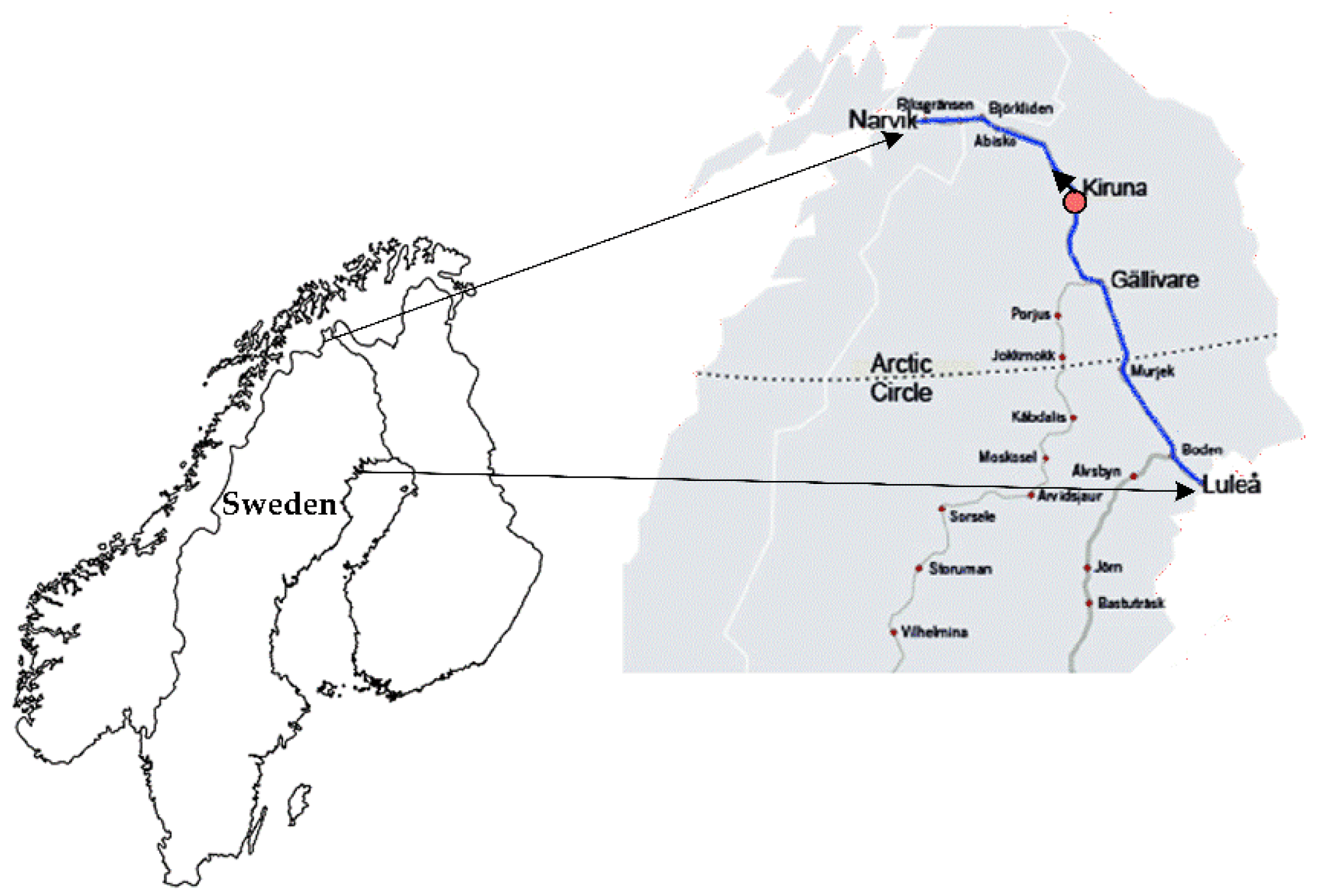
The Iron Ore Line (IOL) is the first longer railway in Sweden which was electrified in 1915. It is a 398 km line that runs between Riksgränsen and Boden, Sweden. The track is designed for single-track use and has a track gauge of 1435 mm. On an average annually, 29 million tons (MGT) of iron ore is transported to the ports of Narvik and Luleå via this line. The maximum allowed speed for an unloaded freight train is 70 km/h and when loaded the allowable speed limit is 60 km/h. For passenger trains, the speed can vary from 120 to 135 km/h.
Figure 3 depicts the geographical location of the Iron line.
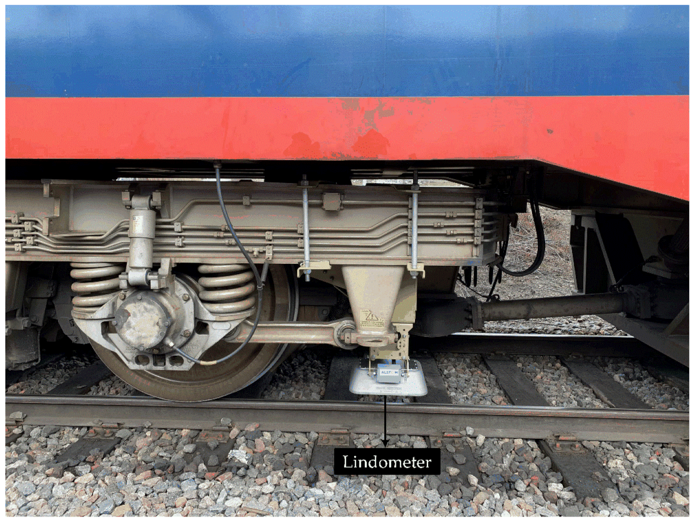
For the present study, the Lindometer was mounted on an unloaded freight train (refer to
Figure 4) and measurements were carried out from Kiruna (depicted in
Figure 3 as a red marker with a black arrow indicating the direction of measurement). The speed of the train was 70 km/h, and the measurement was carried out for a length of approximately 2.5 km. The measurement was recorded using a standard laptop (Dell Ultrabook). The track section considered for this case study had a concrete sleeper with Pandrol fast clip fasteners. The measured track section included one Switch & Crossing (S&C) and one bridge as well as other standard track parts such as insulation joints and welds, etc.
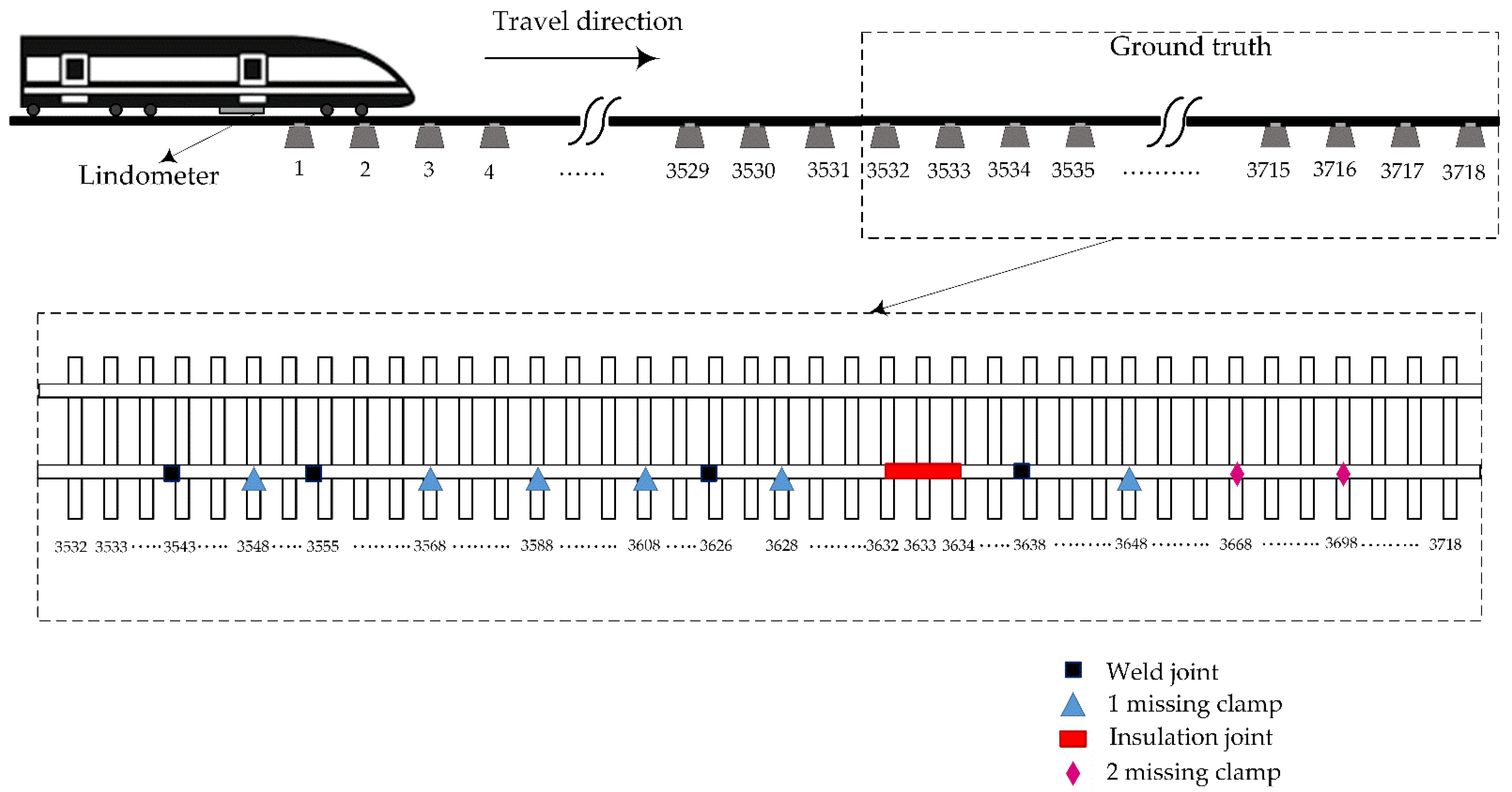
The measured track in this study is depicted in
Figure 5. A total of 3718 sleepers were recorded where the ground truth was inspected for the final 187 sleepers of the section. The ground truth included the position of insulation joints, welds, and missing clamps, etc. In this part, clamps were also manually removed to induce a predefined pattern of fastener anomalies. The section included 172 sleepers with no missing clamps (called healthy fastening system), 6 instances with one missing clamp, and 2 instances where both clamps were missing. The ground truth section also included 4 instances of weld joints and 3 instances of insulation joints.
2.2. Signal Processing and Feature Extraction
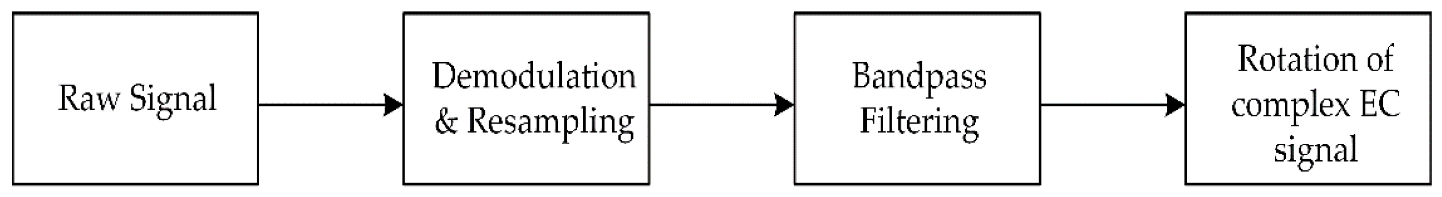
Several signal processing methods were implemented before sufficient information could be extracted from the raw signal, corresponding to the individual fastening system. The EC signal had to be demodulated, resampled, filtered, and rotated to extract relevant features pertaining to the fastening system [
29]. The signal processing techniques employed in this study is depicted in
Figure 6 and a detailed explanation of the same can be found in the previous study [
6,
29].
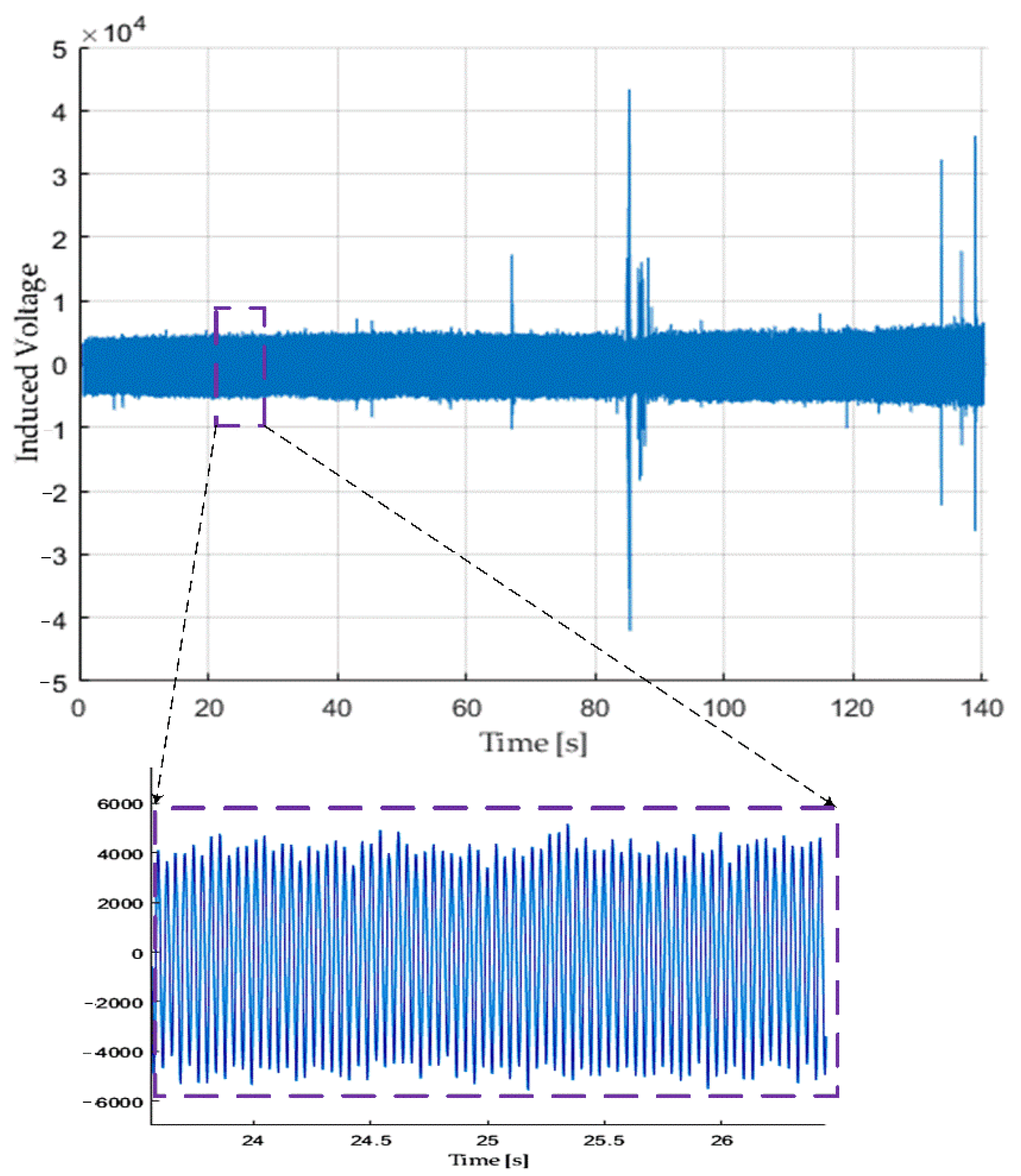
The coil impedance experiences a change when they come in the vicinity of fasteners. The return field from the rail surface modulates the tone from the oscillator. A quadrature amplitude demodulator was used to extract the signal caused by the impedance variation and the raw sensor signal was multiplied by its carrier frequency (27 kHz) and low pass filtered (2 kHz) to extract the baseband. The output from the demodulator is X-axis and Y-axis signals which represent the real and imaginary parts of the impedance, respectively. The signal was then resampled from 215.52 to 35.92 kHz.
After demodulating and resampling the sensor signal, a bandpass filter of lower bound and upper bound of 29 and 34 Hz, respectively, was applied, as the periodicity of the fastener was found to be in this range. The filtering was carried out to retrieve maximum information pertaining to the fastener system and attenuate other frequency components corresponding to noise and other ferromagnetic components.
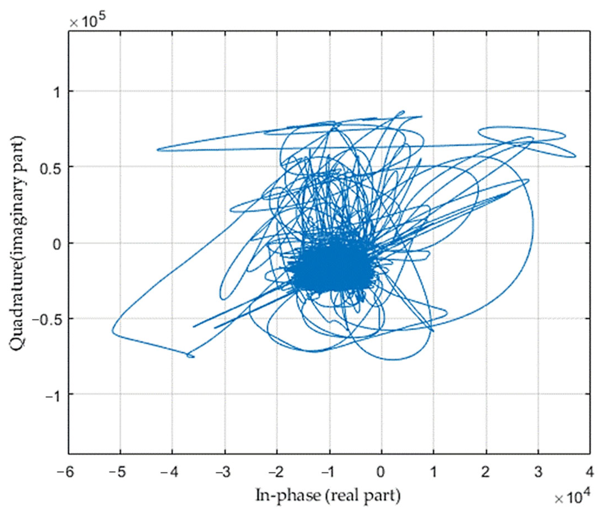
After demodulation, resampling, and bandpass filtering, the fastener signatures in the signal were found to be shifted from the in-phase direction. The complex EC signal was rotated such that the fastener signatures were projected along the in-phase direction to extract maximum information pertaining to the fastener and have better visualization. The EC signal was rotated by degree
θ or
Φ radian, such that the peak amplitude of the fastener signatures was maximized. The signal was rotated by an optimal angle (found from the method employed in a previous study [
29]) of 255° to align the fastener signature along the in-phase direction.
The bandpass filter and the rotation of the EC signals suppress, to an extent, the disturbances arising due to the presence of conductive and magnetic material in the sensor-to-target gap. The bandpass filter was set to extract the fastener signatures and attenuate other frequency components outside that range, which could alter the energy content associated with the fastener signatures. The frequency band for the bandpass filter is dependent on the speed of the train and must be adjusted accordingly. Different components within the railway system have different geometrical shapes, different values of electrical conductivity, and magnetic permeability. Hence, they will occur at a different angle from one another from the in-phase direction compared to the fasteners. Since the study aims to detect fastener signature, the rotation angle was set to align the fastener signatures along the in-phase direction, thus suppressing, to an extent, information from other disturbances.
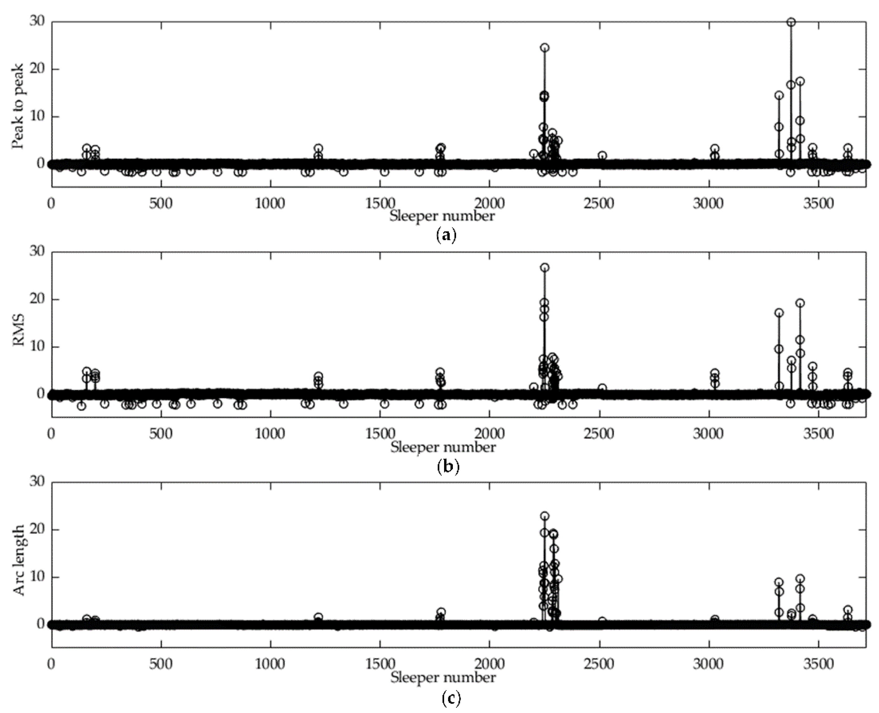
Three features are extracted for the individual fasteners, namely arc length of the complex signal, peak-to-peak, and RMS. The peak-to-peak and RMS feature is obtained from the real part of the EC signal, whereas the arc length feature comprises information from both the real and the imaginary part of the EC signal. A total of 3718 fastener signatures are recorded from the training measurement and thus the feature matrix will have a size of 3718 × 3.
2.3. Anomaly Detection
Anomaly detection refers to the problem of identifying data points, events, and/or observations that deviate from the expected behavior [
32]. These non-conforming points or events or observations are referred to as anomalies or outliers. The general goal of an anomaly detection approach is to define a region representing the normal behavior and identify other observations in the data set which do not belong to this normal region as an anomaly. One of the main challenges for this approach is the availability of labeled data for the training/validation of models. Based on the availability of the label, anomaly detection is classified into three categories: supervised, semi-supervised, and unsupervised anomaly detection. Models using the supervised anomaly detection technique assume the availability of training data points with labels for both normal and anomalous classes. The major challenge for this method is to obtain labeled data that are accurate and well representative of all types of behavior. Labeling is usually performed manually by human experts and thus requires substantial effort and is cost intensive. Semi-supervised techniques assume that the labels are available only for the normal class during training. The typical approach employed in semi-supervised anomaly detection is to build models for the class corresponding to normal behavior and use the model to identify anomalies during the test stage. Unsupervised anomaly detection techniques, on the other hand, do not require training data and work on the assumption that normal instances are more frequent than the anomalies in the data set. Unsupervised learning does not require human expertise to label the entire length of the data set and are hence more cost-effective.
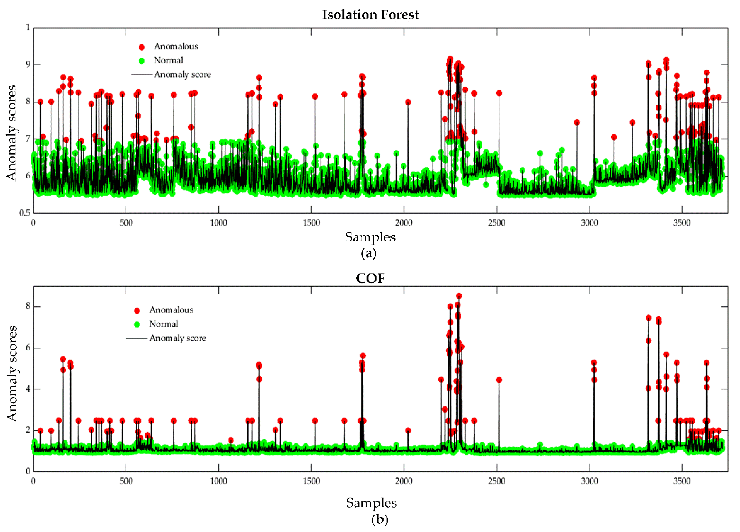
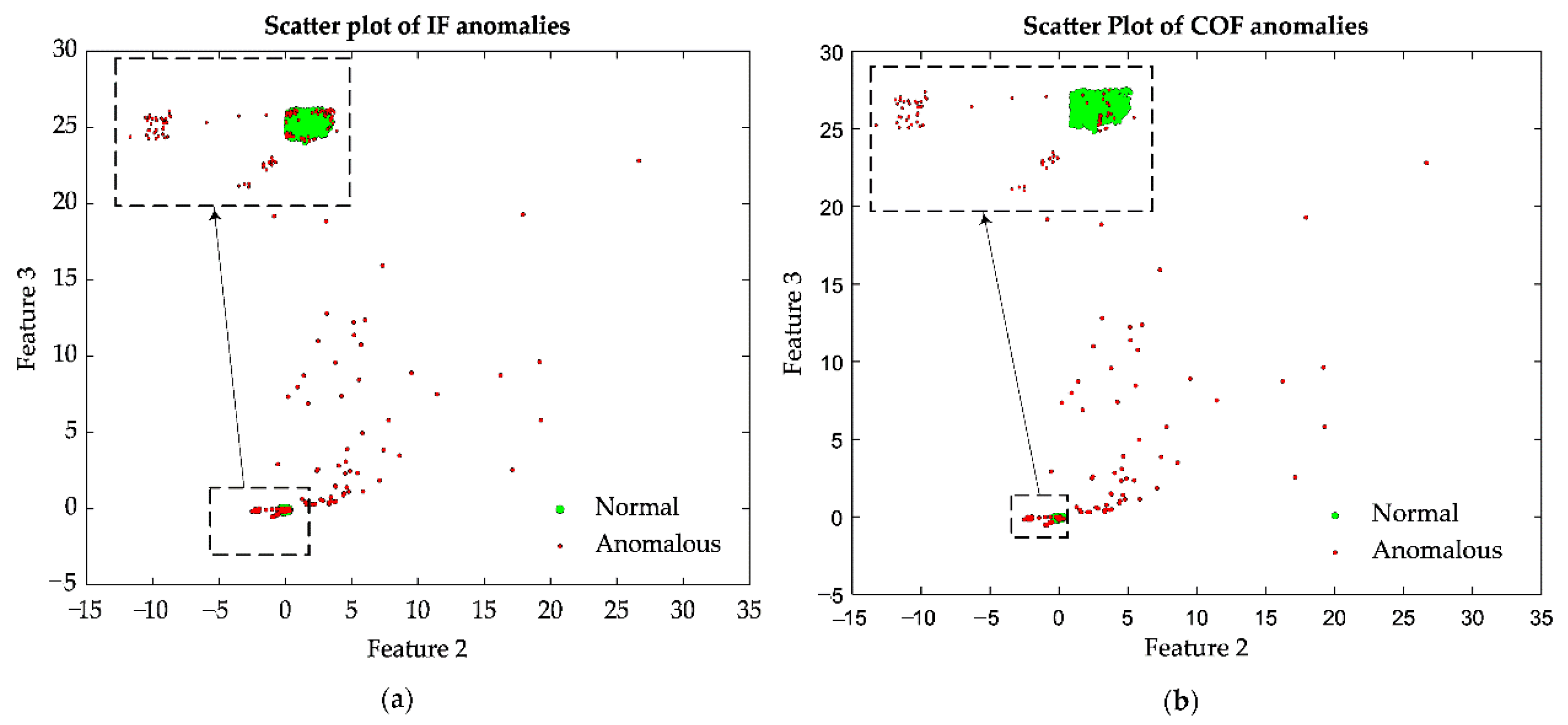
Two forms of unsupervised machine learning techniques are implemented to analyze the fastener measurements. The first model was implemented to identify and segregate the anomalous data points from the healthy or normal ones. The normal behavior in a railway fastening system is when the fastening system has both the rail clamps intact. To segregate the data points to normal and anomalous points, a combination of isolation forest (IF) and connectivity-based outlier factor (COF) were used (briefly discussed below). The two methods were combined to detect both global and local anomalies. The ground truth points were used to evaluate the anomaly detection model based on accuracy, sensitivity, and specificity.
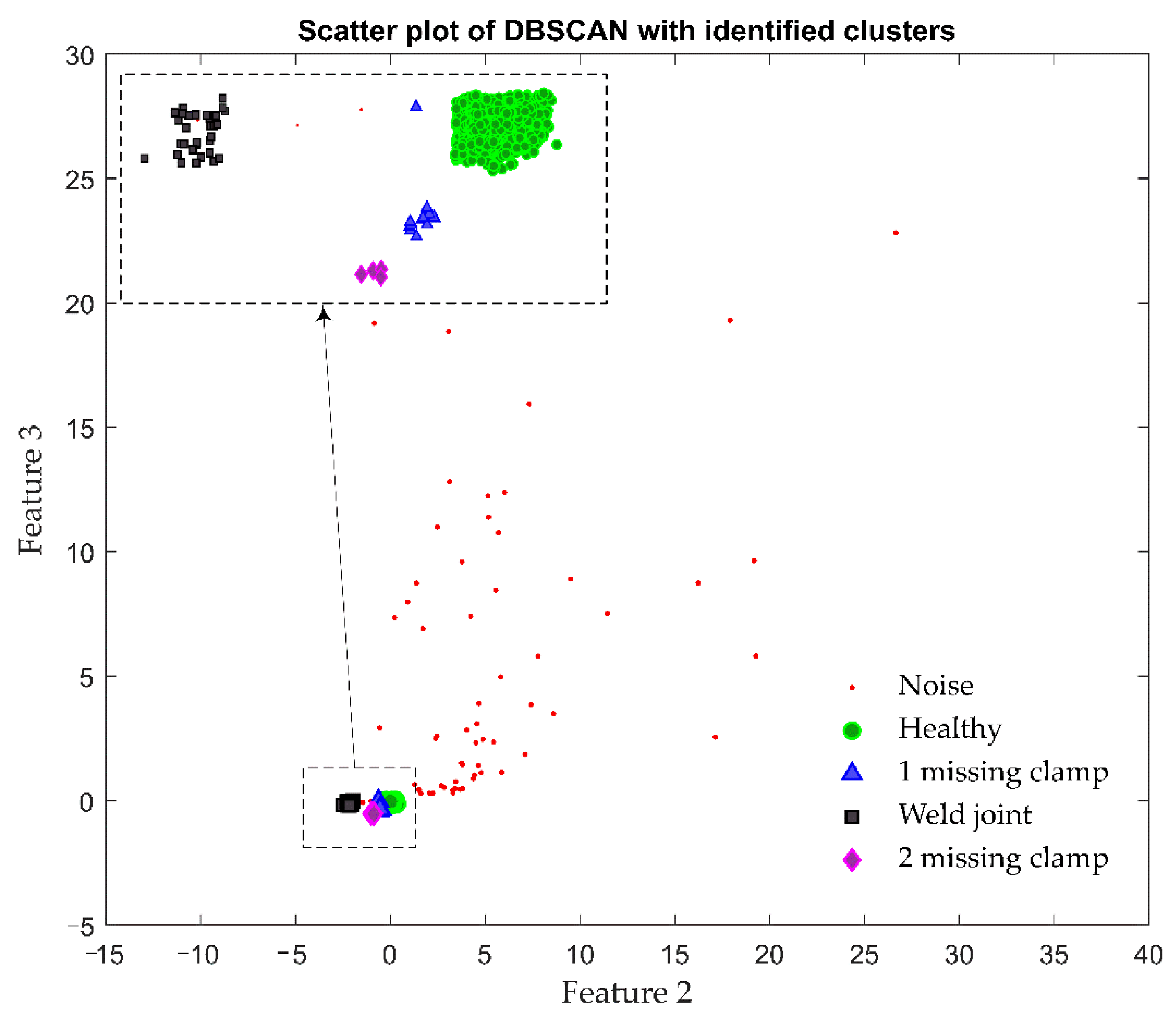
The second method in the anomaly detection model aims to group the anomalous points into meaningful clusters. The clustering was carried out using the DBSCAN algorithm (briefly discussed below). To overcome the problem of identifying what each cluster represents, the authors used a smaller set of data from the measurement where the labels for the data points were known. The smaller set of data was used to identify some or all of the found clusters in order to know what the clusters represented.
2.3.1. Isolation Forest (IF)
The isolation forest is an ensemble-based unsupervised anomaly detection method that is an extension of decision trees. It works on the basis of isolation where iterative partitioning of the input space is carried out to separate a new observation from the rest of the data. The isolation step creates a tree where an observation is present at each leaf and each internal node is associated with a split on one variable. The isolation step is repeated
t times creating different trees. An anomaly score is then generated for each data point by traversing through each tree in the forest. A comprehensive description of the isolation forest is given by F.T. Liu et al. [
33].
2.3.2. Connectivity-Based Outlier Factor (COF)
The connectivity-based outlier factor is an improved version of the local outlier factor (LOF) [
34] where a degree of outlier is assigned to each data point. This degree of outlier is called the connectivity-based outlier factor. The main difference between LOF and COF is the computation of neighborhood
k. LOF computes the neighborhood using Euclidean distance, whereas COF uses the short path method called the chain distance to calculate the nearest neighbors. Once the neighborhood is computed, an anomaly score is generated for each data point. A comprehensive description of COF is given by Tang et al. [
35].
Isolation forests are sensitive to global anomalies and may often find it difficult to detect local anomaly points. COF is sensitive to local anomalies and may have difficulties in detecting global anomalies. An effective anomaly detection algorithm should be able to detect both global and local anomalies. In most cases, if the chosen algorithm is effective in finding global anomalies, then they fail to determine local anomalies and vice versa [
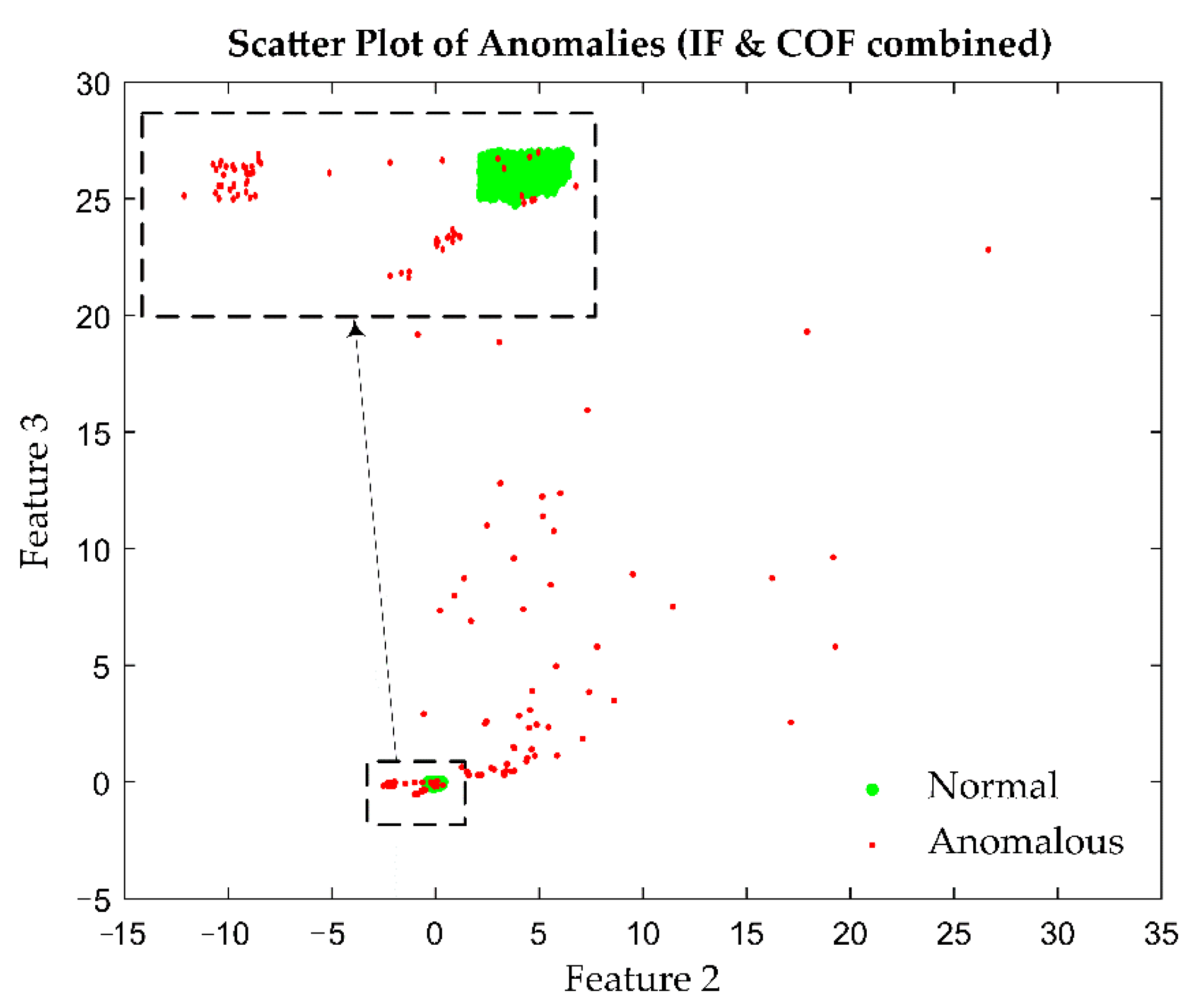
36]. To overcome the problems associated with this problem, an integrated approach using both isolation forest and connectivity-based outlier factor is used in this study. A point is considered as an anomaly only when the point is detected as an anomaly by both algorithms.
As per the guidelines laid down by the Swedish transport administration (Trafikverket), no more than 4 clamps can be missing within a distance of 20 sleepers (20 sleepers × 4 clamps/sleeper = 80 clamps). This accounts for 5% of tolerance in missing clamps over 20 sleepers. This information is used to set the threshold value for the anomaly scoring for both the above algorithms.
2.3.3. DBSCAN
Density-based spatial clustering of application with noise (DBSCAN) is an unsupervised density-based clustering algorithm. DBSCAN works well with arbitrary shaped and sized clusters and does not require to pre-specify the number of required clusters. DBSCAN requires two main parameters, epsilon (
ε) and the minimum number of points, to form clusters of the dense region. Epsilon represents the maximum radius of the neighborhood and minimum points specify the minimum number of data points within the radius of the neighborhood. The closely packed points group together and form a cluster and the points that are in low-density regions are marked as noise. A comprehensive description of the DBSCAN algorithm is given by Ester et al. [
37].
4. Conclusions and Future Work
In previous studies [
6,
29], the authors proposed an alternate approach using a train-based differential eddy current sensor for fastener inspection that can overcome major challenges associated with automated visual inspection systems. This paper presents an automated train-based measurement system with the aid of unsupervised machine learning approaches to facilitate reliable and effective monitoring of railway fasteners by reducing human biases and error for detection of the state of railway fastening systems. The data set used for this study was obtained from an actual train measurement along a heavy haul line in the north of Sweden, where the measurement system was installed on a freight train and where the fastener condition and other likelihood of disturbances were unknown. Unsupervised machine learning models were adopted in this study for detecting and analyzing the underlying patterns and relationships in the data collected.
An anomaly detection model combining isolation forest and connectivity-based outlier factor was proposed to detect anomalies from the data set and to segregate them from the normal or healthy class. The performance of the proposed detection algorithm was evaluated on the ground truth data points, whose label pertaining to their specific condition was known. The proposed method had higher accuracy, sensitivity, and produced significantly fewer false negatives than when IF and COF were utilized individually. The proposed combined IF and COF method was also able to detect all the anomalous points precisely. To segregate the anomalies, a clustering method using the DBSCAN algorithm was also implemented on the data set. DBSCAN yielded four clusters including the healthy or normal cluster. The normal cluster was identified by combining system knowledge and the results or information received from the previous anomaly detection model. To interpret the remaining clusters, the ground truth points were utilized, and the results show that the model was able to segregate a healthy fastening system from other anomalies. Furthermore, the model was able to efficiently detect missing clamps (both one and two missing clamps within a fastening system) and weld joints and segregate them with distinct boundaries. Around 1.72% (64 samples) of the total samples were marked as noise during the clustering method. The noise in the measurement can correspond to various other track components (such as insulation joints, switches, and crossings, etc.) that exhibit different magnetic properties compared to those of fasteners. Future research will make use of features relevant to such components and, by considering the angle of rotation pertaining to such components, further segregate these noises into meaningful clusters.
The current study incorporates only one type of fastener, namely the Pandrol fast-clip. Future studies will also focus on detecting different types of fasteners that can be categorized by the rotation angle, as different fasteners have different geometrical shapes. Future research will also include high-speed measurements, detection of other magnetic track components, detection and quantification of rail defects, and development of efficient condition monitoring techniques with the use of artificial intelligence to detect and predict degradation and faults from big data. The features utilized for this study are subjected to change when the distance between the sensor and the target object varies (i.e., liftoff effect). Liftoff for this application can occur due to wheel wear of the train. However, this is a slow occurring process that can be handled by continuous automatic calibration of the system where the clusters formed by the healthy signatures are used as a reference. This study will be carried out in future work.


