A Probabilistic Analysis of the Switchgrass Ethanol Cycle

Department of Petroleum and Geosystems Engineering, The University of Texas at Austin, TX 78712, USA
Sustainability 2010, 2(10), 3158-3194; https://0-doi-org.brum.beds.ac.uk/10.3390/su2103158
Submission received: 24 August 2010
/
Revised: 26 September 2010
/
Accepted: 29 September 2010
/
Published: 30 September 2010
(This article belongs to the Special Issue Renewable Agriculture)
Abstract
:The switchgrass-driven process for producing ethanol has received much popular attention. However, a realistic analysis of this process indicates three serious limitations: (a) If switchgrass planted on 140 million hectares (the entire area of active U.S. cropland) were used as feedstock and energy source for ethanol production, the net ethanol yield would replace on average about 20% of today’s gasoline consumption in the U.S. (b) Because nonrenewable resources are required to produce ethanol from switchgrass, the incremental gas emissions would be on average 55 million tons of equivalent carbon dioxide per year to replace just 10% of U.S. automotive gasoline. (c) In terms of delivering electrical or mechanical power, ethanol from 1 hectare (10,000 m) of switchgrass is equivalent, on average, to 30 m of low-efficiency photovoltaic cells. This analysis suggests that investing toward more efficient and durable solar cells, and batteries, may be more promising than investing in a process to convert switchgrass to ethanol.
1. Introduction
This paper applies the universal laws of mass and energy conservation to an annual cycle that uses switchgrass to produce ethanol and compares that cycle with the solar photovoltaic cells that deliver equivalent mechanical power. A switchgrass-ethanol cycle consists of two parts: (1) Repeated harvests of switchgrass grown on large industrial plantations, followed by drying, compacting and baling the harvested grass, and transporting the bales to a remote refinery. (2) Repeated decomposition and fermentation of the switchgrass feedstock, followed by membrane separation/distillation/azeotrope separation of a dilute ethanol broth to give anhydrous ethanol. In the refinery, switchgrass is used as both the feedstock for “cellulosic ethanol” fuel and the sole source of heat and electricity required to run the grass decomposition, simple sugar fermentation, and ethanol distillation processes. Both parts of the cycle are repeated each year and deliver a specified volume of anhydrous ethanol continuously for decades.
The term “cellulosic ethanol” is meant to suggest that certain components of wood and green plant materials (cellulose, pectins, and hemicelluloses) are chemically separated (mostly from lignin in wood) and partially split into hexose and pentose monomers, which are then fermented to produce ethanol.
Close to three billion years of plant evolution from cyanobacteria and algae have made cellulose very stable and resistant to biochemical attacks [1,2]. Cellulose can be quickly decomposed and hydrolyzed by extreme mechanical grinding, hard nuclear radiation, or steam exploding and severe chemical attack by hot concentrated sulfuric acid or sodium hydroxide [3,4,5,6,7,8]. Biochemical enzymatic attacks are orders of magnitude slower and have an inherently low efficiency [9,10]. For example, it takes 20 hours of a cellulase enzyme attack to shift to a homogeneous reaction kinetics and 90 hours to complete the attack. When strong acids or hydroxides are used to damage the crystalline structure of cellulose, reaction kinetics accelerate by two orders of magnitude, i.e., the reaction time is shortened by a ratio comparable to the speed ratio of jet-flying and human jogging.
Cellulose fibers are separated from the rest of woody biomass in the well-known “kraft-process” that is fast, efficient, and highly energy intensive. The kraft process, developed by Carl Dahl in 1884, now produces 80% of paper volume. Caustic sodium hydroxide and sodium sulfide are applied to extract the lignin from the wood fiber in large pressure vessels called digesters. The best energy efficiency of this process is ∼30 MJ/kg of paper pulp [11], more than the higher heating value of pure ethanol, defined in Section 3.4 Therefore a much milder, but slow enzymatic process must be used to obtain simple sugars from cellulose.
It has been claimed that over 1 billion tons of cellulosic biomass can be extracted from the U.S. territory each year [12,13], and converted into biofuels, e.g., 130 billion gallons of cellulosic ethanol [14]. Alas, the recent Moderate-resolution Imaging Spectroradiometer (MODIS) satellite-based [15] calculations [16,17] of net primary productivity of all plants growing in the U.S. cast doubt on the sustainability of this claim. To produce 130 billion gallons of ethanol, one would have to use each year between 1/3 and 2/3 of all above-ground biomass growth in the U.S.
It is customary in the agricultural literature, e.g., [18,19,20,21], to conduct a few short-term (<5 years) field studies and assume that average yield of switchgrass anywhere in the U.S. can be quantified by a single number x ± some deviation, and that number can only grow with time. The x estimated by Schmer et al. from their field data [21] was 7.2 Mg ha yr. In this paper it is suggested that the wide temporal and spatial variations of switchgrass yields prohibit relying on a single x. Instead, using all available data weighted by a long-term field survival function, one can propose a probability distribution function of continuous (or eternal) switchgrass yields, and calculate this distribution’s expected value. That value alone (calculated in this paper to be 6.8 Mg ha yr) is unreliable, but the distribution provides a qualitative insight into what might be expected from the future switchgrass plantations. Quantitative models of complex processes on the surface of the Earth do not work, as illustrated in detail by the Pilkey and Pilkey-Jarvis [22]. On the other hand, a qualitative model when applied correctly in what-if scenarios, can be useful. A brief look back at the simplistic quantitative models of the corn ethanol industry (e.g., The Greenhouse Gases, Regulated Emissions, and Energy Use in Transportation Model (GREET) [23] and its conceptual offspring, the Berkeley’s Energy Resources Group Biofuels Analysis Meta-Model (EBAMM) [24,25]), have been shown to be not only physically incorrect, e.g., [26], but also incapable of predicting the odds of survival of ethanol companies, which have been completely dependent on government subsidies regardless of the market conditions.
To calculate a realistic efficiency of conversion of switchgrass to ethanol, I “reverse-engineer” an estimate of the energy efficiency of cellulosic ethanol production in an existing pilot plant, operated by Iogen in Ottawa, Canada. I then translate the Iogen plant results from wheat straw to switchgrass and calculate how much additional switchgrass must be burned to obtain anhydrous ethanol with “zero” use of fossil energy. To account for all available field data on switchgrass yields, I perform a regression (“Monte Carlo”) analysis. Finally, I compare the switchgrass-ethanol cycle with photovoltaic cells.
Similar mass, energy [26,27,28], and free energy (exergy) [16,29,30,31] balances have been applied elsewhere to various crops and biofuels. Free energy is irreversibly consumed in all steps of all biofuel production processes and should be used to determine the relative degrees of unsustainability of different biofuels. Such applications are always based on physical data, including the repeated average yields of a plant feedstock grown on large fields, and the measured energy efficiency of ethanol refineries, or cogeneration plants using biomass gasification/liquid fuel synthesis and generating electricity.
2. Preliminary Calculations
By assuming the average switchgrass yield from Schmer et al. [21], doubling the energy efficiency of cellulosic ethanol refinery relative to that from Farrell et al. [24,25], and disregarding the high chemical and environmental costs of large-scale switchgrass agriculture, one does not obtain a viable macrosystem of automotive fuel supply. One should therefore consider other more efficient technologies of converting sunlight into motive power. The simple calculation below demonstrates this fact.
Assuming average continuous (“eternal”) yield of switchgrass of 7.2 tons per acre per year on dry mass basis (dmb)—corresponding to the estimate by Schmer et al. [21]—a biorefinery that might one day process 2,000 tons dmb of switchgrass per day [32], will need 101,000 acres of grassland to supply it with raw material. (Epplin et al. [32] assume 5.5 tons dmb/acre as their average switchgrass yield.) Assume that the supply area is (1) roughly a circle with the biorefinery at the center, and (2) the dry switchgrass is compacted to high density bales and transported by large trucks. Then roughly 400 truck trips, 2 × 8 km long on average, will be required each day. Eight km is the mean square radius that scales the field area encompassed by the circle. Note that the real distance driven by the trucks will always be longer, because one cannot fill 100,000 acres of land with a contiguous sea of switchgrass. Meandering roads, buildings, ponds, creeks, rivers, perhaps even trees, will add more area. At 2.4 km/L, these trucks will use about 980,000 liters of diesel fuel per year. As discussed later in this paper, the energy requirements of a switchgrass refinery might be satisfied by burning more switchgrass, but—because of the complex transportation logistics and the doubling of field area involved—coal or natural gas use will be more likely. Let us set aside the different estimates of process energy requirements of the non-existent switchgrass refinery (29 MJ/L in EBAMM [24,25]). Instead, let us assume that this refinery is 43% energy-efficient, requiring only 15 MJ of primary energy per liter of ethanol, just as the modern corn ethanol refineries compared in Figure 2 in [28]. Also assume the ethanol production efficiency from EBAMM, 0.38L/kg switchgrass, [26,33]. With these assumptions, our biorefinery will produce 3,000 barrels or 493,000 L of gasoline equivalent per day, and will need 360 tons of coal equivalents per day. At 57 L (15 gallons) of gasoline equivalent per tank (equal to L of ethanol per tank), and assuming that a car drives for one week on a fuel tank, our switchgrass biorefinery will be able to fill up tanks of 59,400 small and midsize cars each year (cars that use on average 11 L of gasoline equivalent per 100 km or 22 miles per gallon), provided that the switchgrass yield remains perfectly constant. To put it differently, one will need 1.7 acres of switchgrass and 2.2 tons of coal equivalent/year to run a midsize car in perpetuity. If one covered these 1.7 acres of land with 10%-efficient solar photovoltaic cells (also an impossible task today), one would generate primary energy sufficient to run 115 cars. Thus, one obtains a factor of roughly 100 when comparing the future energy efficiencies of the solar cell—and switchgrass ethanol-driven car systems. The simplified analysis here has neglected the energy costs required for the production of switchgrass; harvesting, compacting and baling switchgrass; producing and maintaining photovoltaic cells; and maintaining the transportation/distribution infrastructure. It turns out [16] that after these costs are included, the photovoltaic car systems are 100 to 1,000 times more efficient than the different biofuel car systems.
In the metropolitan San Francisco Bay Area, there are 4 million vehicles, see Table A-5 in www.mtc.ca.gov/maps_and_data/datamart/forecast/ao/aopaper.htm (note the two underscores). Thus, with the very optimistic assumptions above, roughly 7 million acres of switchgrass and 8 million tons of coal equivalent per year (∼1 % of U.S. coal production), would be required to fuel the Bay Area’s vehicles. Seven million acres is equal to 9% of the total area of corn agriculture, by far the largest agricultural crop in the nation that delivers more biomass than all other crops combined. Seven million acres is also 2% of all grassland area in the U.S., see Table 2.3 in [17], and is 80% of the 9 million acres of prime irrigated agricultural land in California, see Edward Thompson, Jr., American Farmland Trust, July 2009, www.farmland.org/documents/AFT-CA-Agricultural-Land-Loss-Basic-Facts_11-23-09.pdf.
Note that if one went back to EBAMM for the refinery efficiency, one would need 16 million tons of coal equivalent per year to power the vehicles in a single major metropolitan area in the U.S. If, in addition, one recognizes that the EBAMM ethanol yield o 0.38 L/kg has no factual justification, see Section 3.4, and 0.23 L/kg is appropriate, these requirements will grow to 11.6 million acres and exceed 16 million tons of coal equivalent (∼2% of U.S. coal production in 2008), respectively.
A vast acreage of switchgrass would encompass highly varied climactic conditions and soils, undoubtedly lowering the current average yield estimates. For example, corn yields in Minnesota are usually 50% higher than those in Missouri. The same general principle will apply to switchgrass grown in different regions of the U.S. Two numbers for average yield of switchgrass and refinery efficiency, presented in [21] and [24,25], are inadequate to describe such a complex distributed system. Here I attempt to fix this deficiency by providing contexts of the means and standard deviations of switchgrass yields and refinery efficiencies.
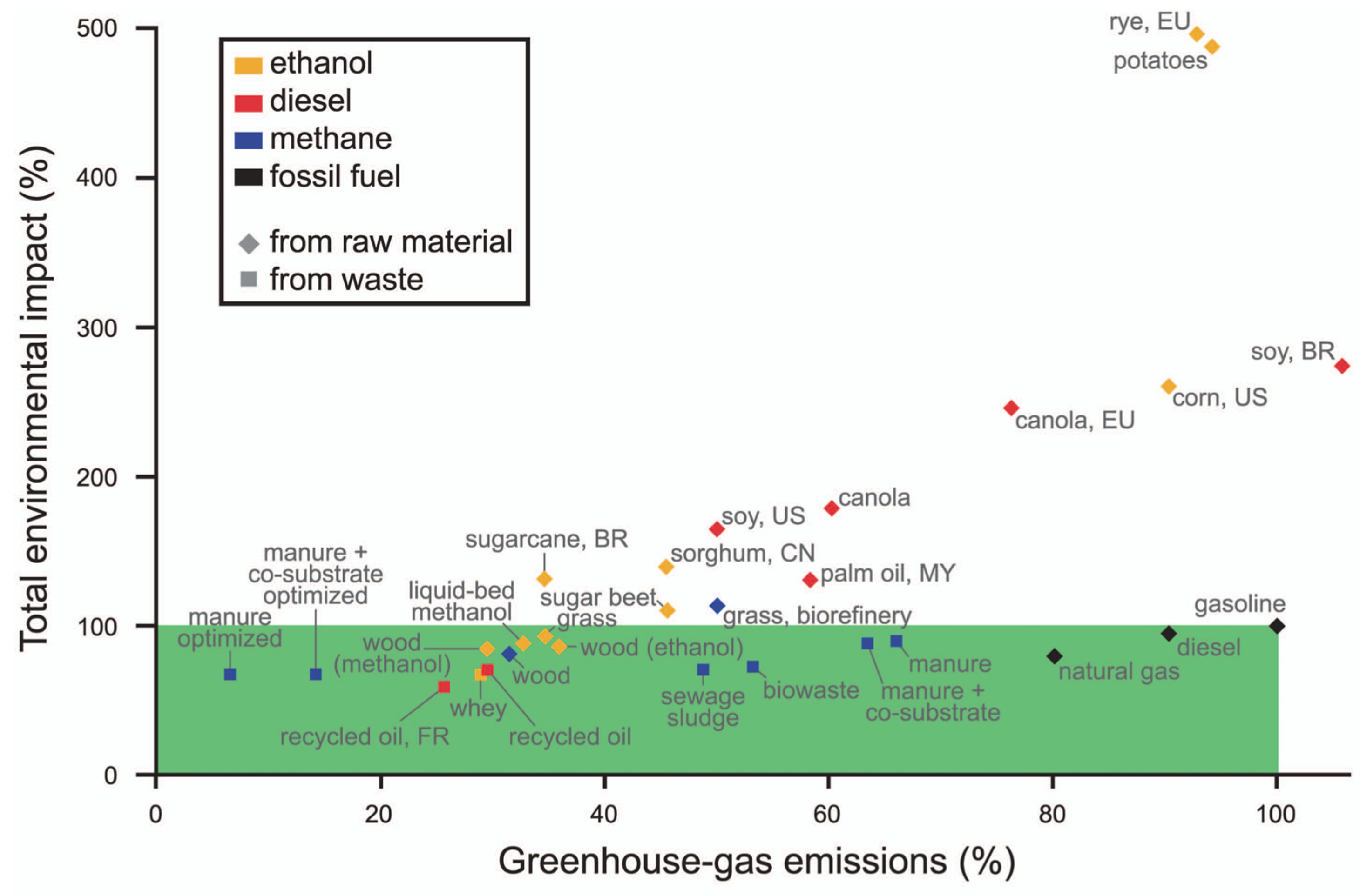
Figure 1 is reproduced from the Supporting Online Materials (SOM) of [34]. This figure summarizes the environmental impacts of 29 major biofuel schemes. The bottom line is this: the large-scale biofuel systems have very large negative impacts on the entire planet that go well beyond those of natural gas and crude oil. In addition, our planet can never produce enough of the raw biomass for these systems for a sufficiently long time, see e.g., [17], regardless of the claims by Perlack et al. [12].
Figure 1.
Greenhouse-gas emissions are plotted against overall environmental impacts of 29 transport fuels, scaled relative to gasoline. The origin of biofuels produced outside Switzerland is indicated by country codes: Brazil (BR), China (CN), European Union (EU), France (FR), and Malaysia (MY). Fuels in the shaded area are considered advantageous in both their overall environmental impacts and greenhouse-gas emissions. Adapted from [35].

3. Input Data
3.1. Switchgrass Yields
Here, the published switchgrass yields are compared and analyzed. In particular, a distinction is made between (a) the finite-time switchgrass plantations that take 1— 3 years to establish and are commercially viable for 5–20 years at variable yields, and (b) the “eternal” average yield of switchgrass needed for the robust, multi-decade fuel supply estimates.
All plant mass is reported on a water-free basis. Switchgrass (Panicum virgatum) is a warm season C grass and a close cousin of corn (maize) [36]. It is one of the dominant species of the central North American tallgrass prairie. Switchgrass is a hardy perennial that reproduces by rhizomes, shoots (tillers), and seeds. In my calculations I assume that switchgrass begins growth in late spring, takes only 1–2 years to grow sufficiently to establish a harvestable field, and may last for another 8, and perhaps even 19 years.
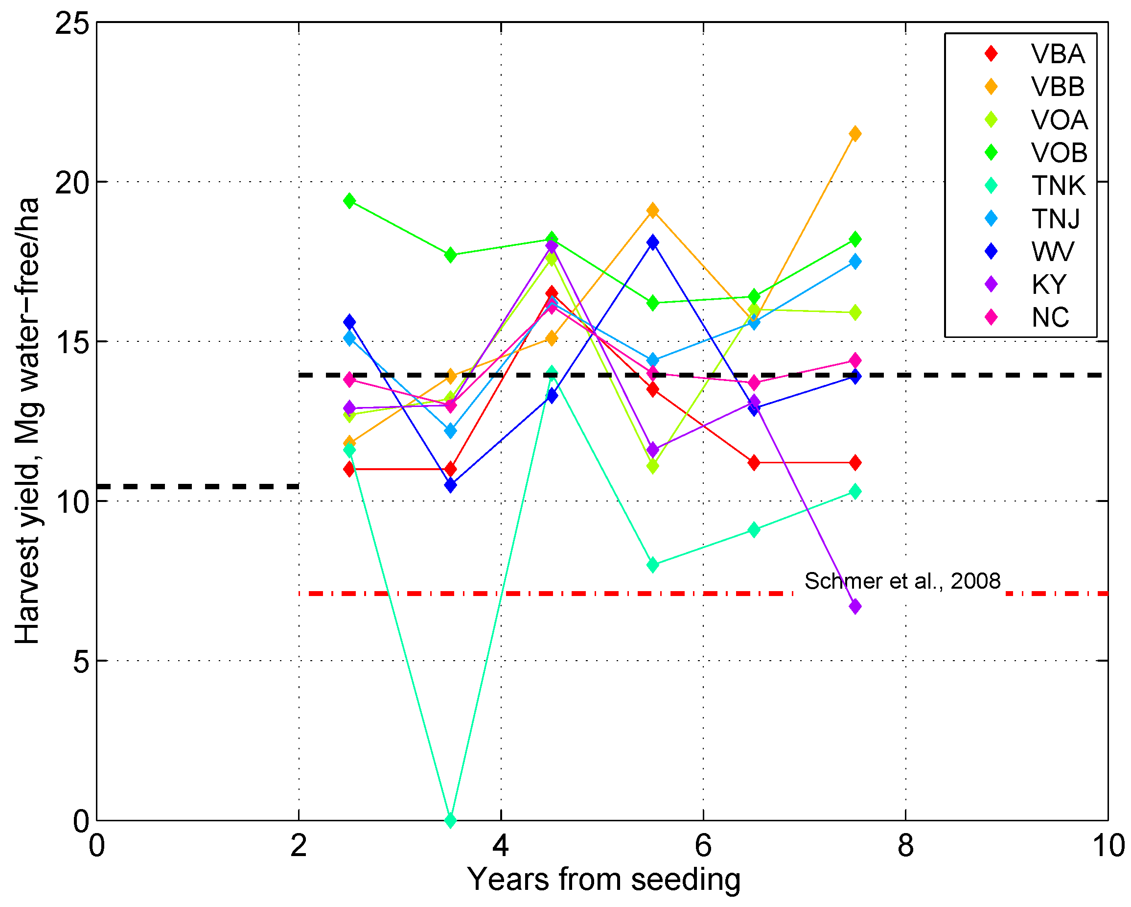
On tiny, m and m, plots fertilized similarly to corn fields, switchgrass can yield from 4 to 18 Mg ha y for 4 years, as reported by Casler & Boe [19]. Larger switchgrass stands have been investigated for at least 10 years in one case [37], but seldom above 5 years [38]. The field studies in [18,19,20,21,37] are summarized in Figure 2, Figure 3, Figure 4, Figure 5 and Figure 6. The reported mean harvests vary from 4 to 25 Mg ha yr and the stand establishment periods vary from 1 to 3 years.
Figure 2.
Single crops of switchgrass on large fields in Virginia, Blacksburg, Site A and B (VBA, VBB); Virginia, Orange, Site A and B (VOA, VOB); Tennessee, Knox (TNK) ; Tennessee, Jack (TNJ); West Virginia (WV); Kentucky (KY); and North Carolina (NC). The upper broken line represents the mean of the data, the lower one is the continuous average with a 2-year delay of annual harvests. Source: Parrish et al., [18].

Figure 3.
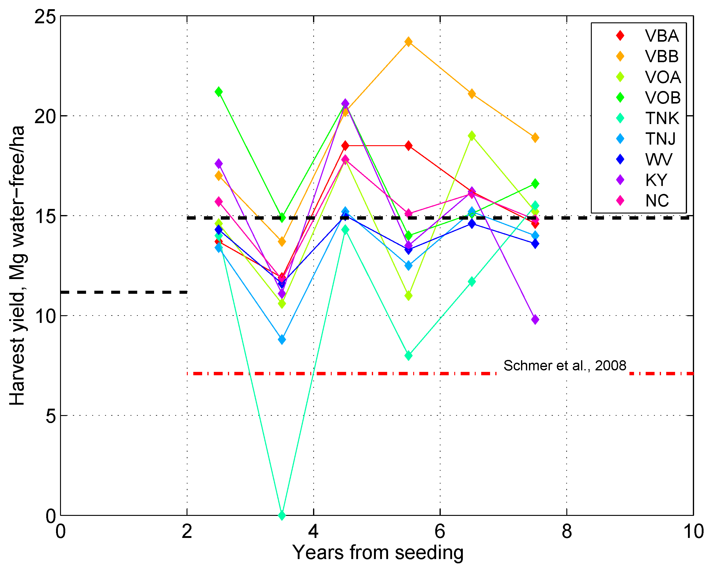
Double crops of switchgrass on large fields in Virginia, Blacksburg, Site A and B; Virginia, Orange, Site A and B; Tennessee, Knox; and Tennessee, Jack. The upper broken line represents the mean of the data, the lower one is the continuous average with a 2-year delay of annual harvests. Source: Parrish et al., [18].
Figure 3.
Double crops of switchgrass on large fields in Virginia, Blacksburg, Site A and B; Virginia, Orange, Site A and B; Tennessee, Knox; and Tennessee, Jack. The upper broken line represents the mean of the data, the lower one is the continuous average with a 2-year delay of annual harvests. Source: Parrish et al., [18].

Figure 4.
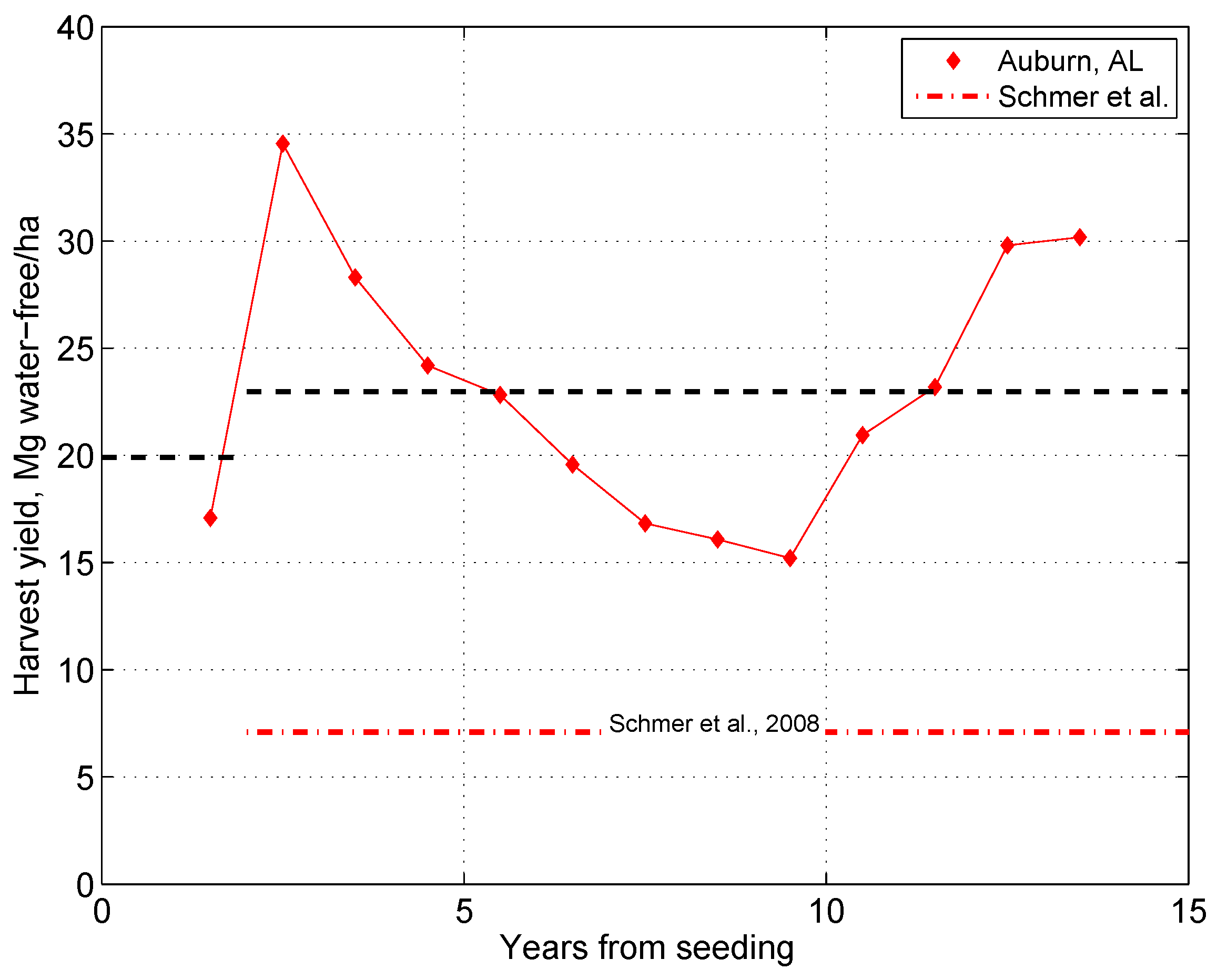
A 10-year study of switchgrass growth in Auburn, Alabama. The upper broken line represents the mean of the data, the lower one is the continuous average with a 2-year delay of annual harvests. Source: McLaughlin & Adam Kszos [37].
Figure 4.
A 10-year study of switchgrass growth in Auburn, Alabama. The upper broken line represents the mean of the data, the lower one is the continuous average with a 2-year delay of annual harvests. Source: McLaughlin & Adam Kszos [37].

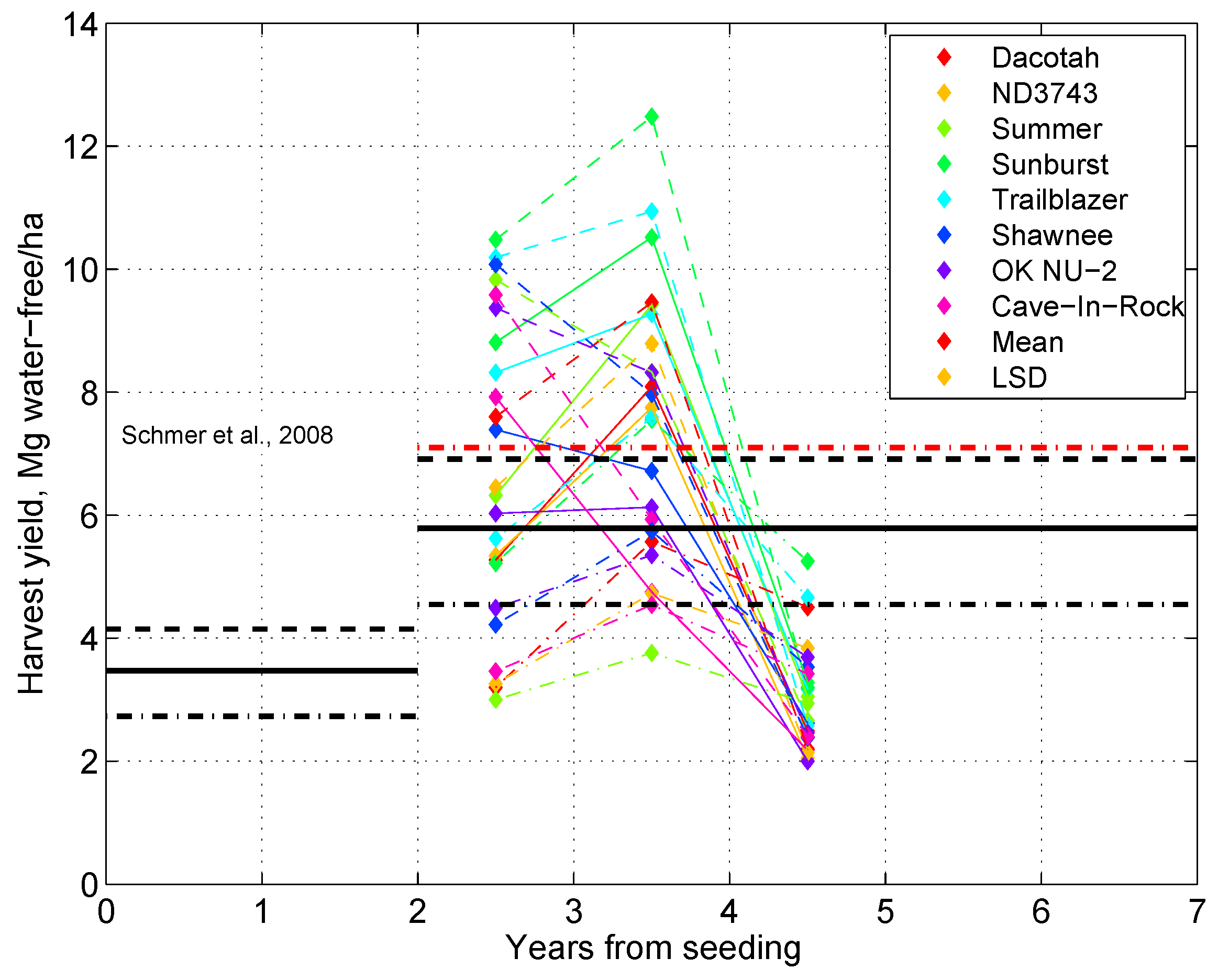
Figure 5.
Measured yields of 8 switchgrass cultivars (diamonds) at three North Dakota sites. The continuous lines refer to the Mandan Site 1, the broken lines to the Mandan Site 2, and the dash-dot lines to the Dickinson site. Those sites were small, roughly m. The upper horizontal lines represent the means of the data and the lower ones are the continuous average with a 2-year delay of annual harvests. Note that these yields extrapolate to zero in up to 7 years. Source: Berhdal et al., [20].

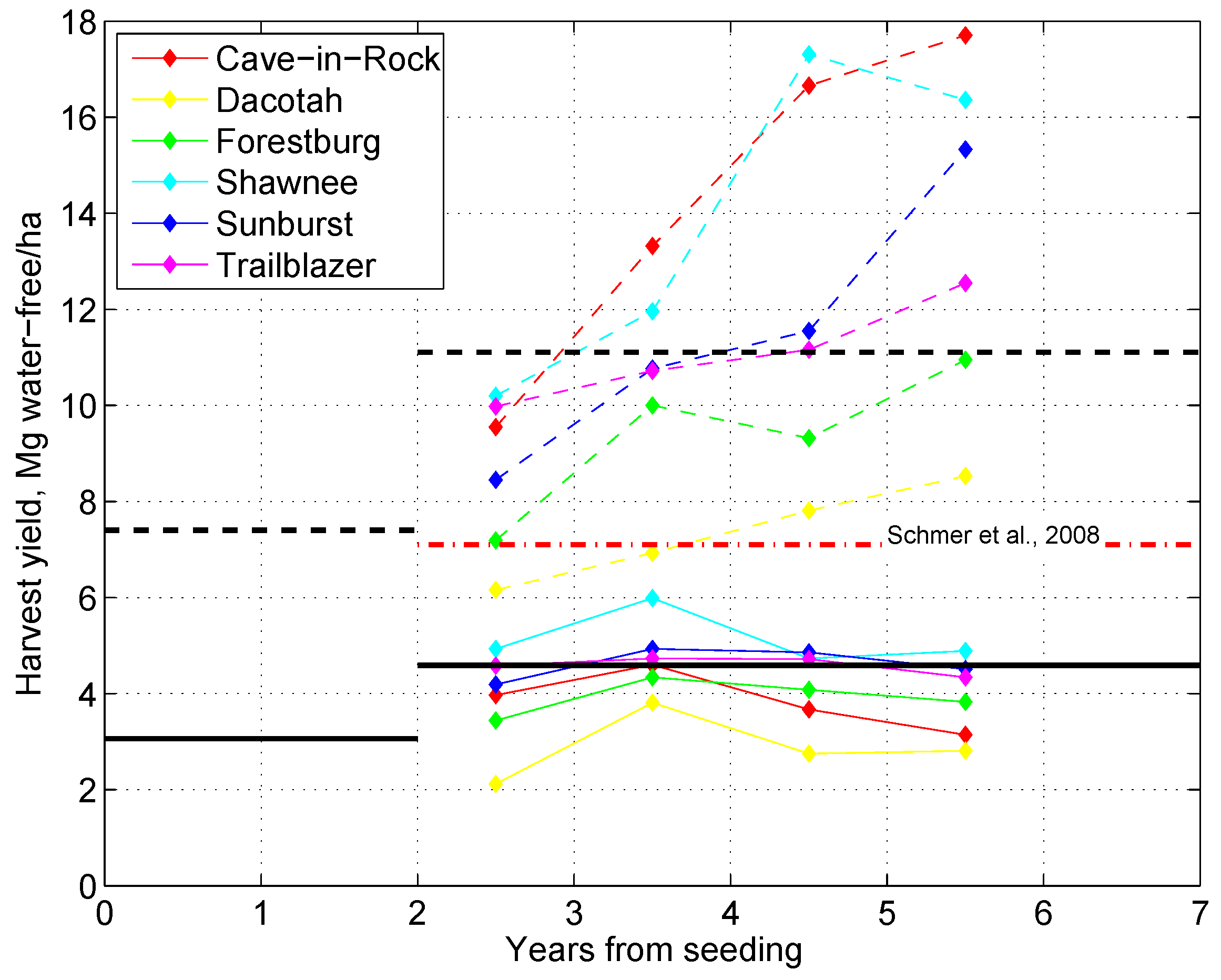
Figure 6.
Measured yields of 6 switchgrass cultivars (diamonds) at a Brookings, SD, and Arlington, WI, sites. Plot sizes were tiny, 1.6 × 3.0 m at Brookings (continuous lines) and 1.6 × 1.8 m at Arlington (broken lines). The upper horizontal lines represent the means of the data and the lower ones are the continuous averages with a 2-year delay of annual harvests. Source: Casler and Boe, [19].

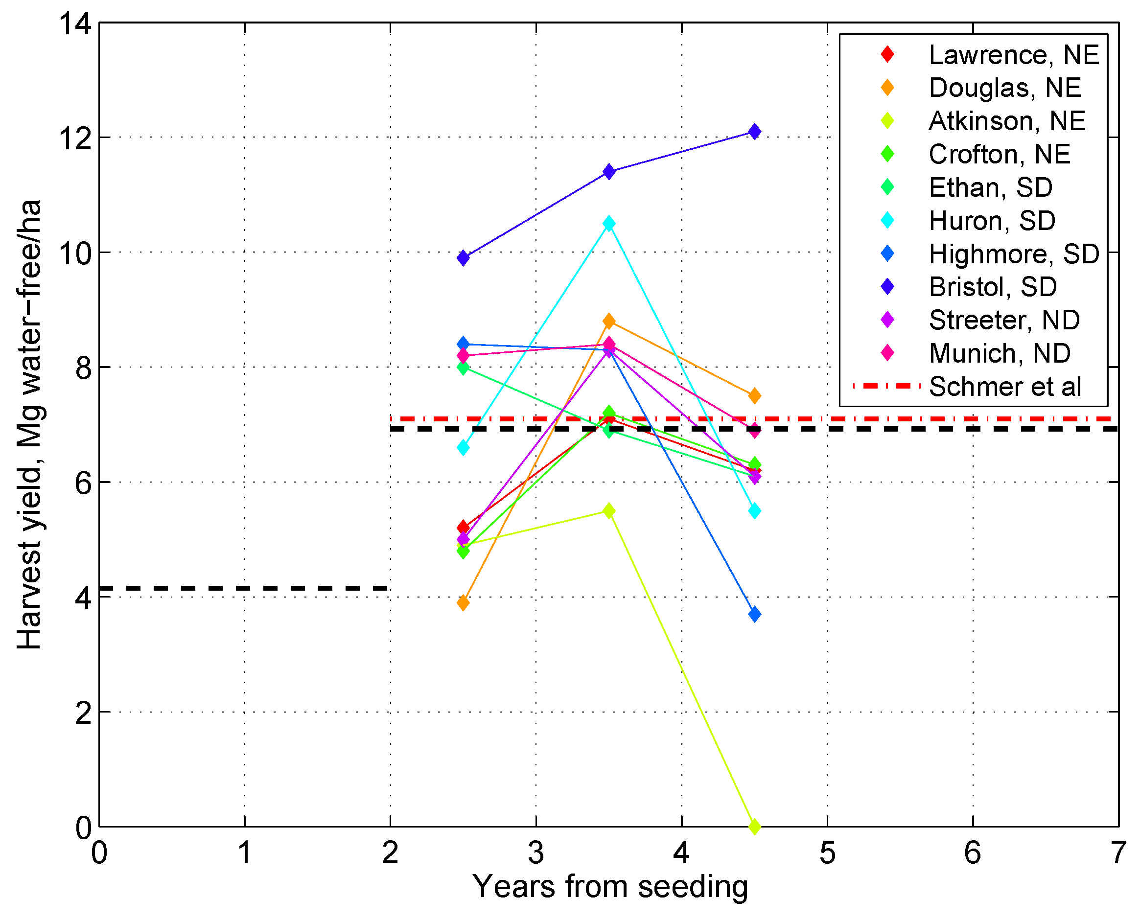
Figure 7.
Measured yields of switchgrass (diamonds) established for 2 years on large fields in North Dakota (ND), South Dakota (SD), and Nebraska (NE). The dash-dot thick line is the continuous yield prediction from [21]. The upper broken line represents the mean of the data, the lower one is the continuous average with a 2-year delay of annual harvests. With one exception, these yields extrapolate to zero from 4.5 to 11 years. Source: Schmer et al. [21].

Harvest Delays
What matters from the point of view of transportation fuel supply is the continuous (year-after-year) mean supply of biomass and the variance of this supply. Therefore, taking an arithmetic mean of 3–4 years of harvest would be justified only if switchgrass grew “forever” with the commercially viable fluctuating yields, after it has been established for two years on large fields. Table 4 in the Supporting Information (SI) to Schmer et al. [21] gives a comprehensive overview of the actual biomass yields from 10 established (2 years after planting) large switchgrass fields in the midcontinental U.S. The SI data in Schmer et al. [21] are plotted in Figure 7. It appears all but one of the measured switchgrass yields extrapolate to zero after 4.5 to 11 years from seeding.
If switchgrass is not harvested for 2 years, and the harvest data are reported only for 3 years, then the actual yields should be discounted by taking the mean of
For the data in the SI Table 4 in [21], this procedure discounts the yields effectively by a factor from 3/5 up to 5/7. In contrast, the switchgrass field studied by McLaughlin and Adam Kszos [37] survived at least ten harvests with the yields higher than those in all other studies considered in this paper [18,19,20,21,37,38,39]. In each of the Figure 2, Figure 3, Figure 4, Figure 5, Figure 6 and Figure 7, the mean yields of the harvests, and mean continuous yields with a 2-year delay are denoted by the horizontal broken lines.
My choice of a 2-year delay of annual harvests for the low-yield fields and a 1-year delay for the high-yield ones, is based on the following reports:
- The SOM spreadsheet to [21] contains the following information: “Table 4. Biomass yields from established (2 years after planting) switchgrass fields in the midcontinental U.S.”
- In their paper, Schmer et al. state the following: “At the field scale in the northern Great Plains, second year biomass yields are limited by establishment stands only if initial stands are less than 40%. If establishment year switchgrass stands on a field have threshold frequency levels of 40% or more, post-establishment biomass yields and post-establishment switchgrass stands are likely influenced more by site and environmental variation than by initial stand frequency. Failure to obtain a fully successful switchgrass stand the establishment year (stand frequency of 40% or greater) can limit biomass yield in post-establishment years resulting in decreased revenue.”Since 4/10 sites were below 40% frequency and 7/10 below 50% frequency, I took this finding as a statistically valid restriction to harvesting switchgrass in the first two years after establishment.
- The Barnsby et al. [40] study stated that although switchgrass yields were low in the establishment year (2.44 Mg h), yields increased over the next 4 years showing relatively little response to precipitation. I took their finding as a valid restriction to harvesting switchgrass in the first two years after establishment.
- McLaughlin and Adam Kszos [37] state: “One of the most persistent issues in producing switchgrass as an energy crop has been delineation of management regimes that will enable growers to rapidly and consistently establish strong stands of switchgrass. As a small-seeded species that initially allocates a large amount of energy to developing a strong root system, switchgrass will typically attain only 33–66% of its maximum production capacity during the initial and second years before reaching its full capacity during the third year after planting. Switchgrass is most susceptible to weed competition as well as the dangers of “assumed failure” during the critical first season.” I took their finding as a valid restriction to harvesting switchgrass in the first two years after establishment (emphasis mine).
- Fike et al. [38] state: “Limited information is available regarding biomass production potential of long-term (-yr-old) switchgrass. ...Yields at Site B (19.1Mgha) were about 35% greater than those at Site A (14.1Mgha), although the sites were only 200m apart.” I take this statement to mean that, except for the Auburn study, zero evidence has been gathered thus far about the long-term viability of switchgrass monocultures and that there is a great variability of switchgrass yields. ...“Plots were evaluated in fall 1996 after having been established in 1992 (or 1993 in Kentucky).” (Footnote in Table 2, title of Table 3.) This means a waiting period of 2–3 years.
- Fike et al., [39] state: “During 1992, four switchgrass cultivars were planted at eight sites across five states (Table 1). Sites were chosen to bound broad geographic, edaphic, and climatological differences within the upper southeastern U.S.A....Cutting managements were first imposed in the year after establishment. Biomass yields reported here are based on harvests from 1994 to 1996, with the exception of the Kentucky site (1995 and 1996 only due to later establishment)”. This remark, again, is a clear indication of a 2-3 year delay between regular cutting of switchgrass and stand establishment.
3.2. Inputs to Switchgrass Agriculture
In this section, the average annual mass inputs of macronutrients (NPK and Ca) and field chemicals, such as pesticides, herbicides and fungicides, as well as the corresponding energy inputs to switchgrass agriculture are estimated and discussed.
Switchgrass is in many ways similar to lawn grass. If one bags grass clippings from a lawn, immediately one notices that the lawn starts to become yellow, and the “yield” (the number of times one has to mow) decreases. This declining lawn productivity is caused by the depletion of macronutrients (N, P, and K) and micronutrients. Each time one removes biomass “trash” from an environment, one removes nutrients, and future yields suffer [16]. Switchgrass is exactly the same—if one harvests switchgrass for biomass, fertilizer must be applied each year at levels similar to those applied to corn fields.
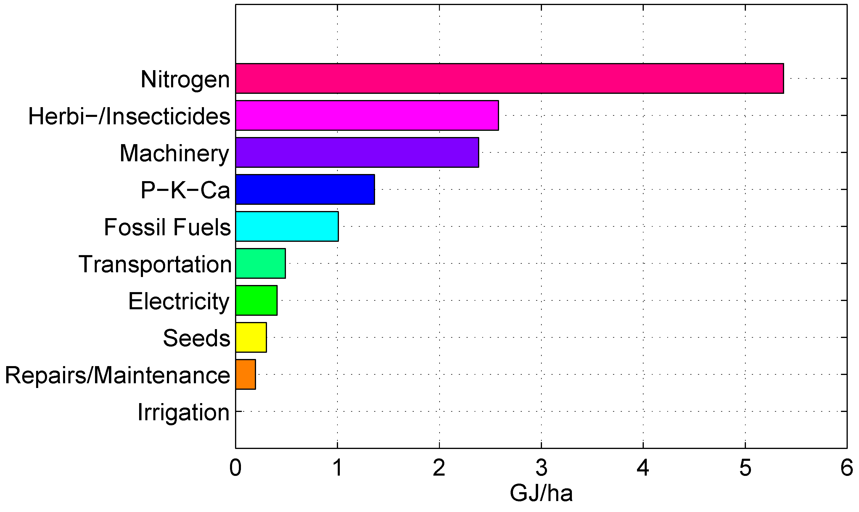
The mass fluxes in industrial switchgrass agriculture and the pertinent references are listed in Table 1. The corresponding energy fluxes are listed in Table 2 and are shown in Figure 8. Note that by accounting for the machinery, repairs, transportation, potash, and lime costs, these energy fluxes are about 47% higher that those listed in the SI to Schmer et al. [21].

| Switchgrass | 6088 | lbm/acre | 6830 | kg/ha-yr |
| Nitrogen | 100 | lb N/acre | 112 | kg N/ha-yr |
| Phosphorus | 13 | lb PO/acre | 14 | kg PO/ha-yr |
| Potassium | 28 | lb KO/acre | 31 | kg KO/ha-yr |
| Lime | 545 | lb CaO/acre | 611 | kg CaO/ha-yr |
| Gasoline | 0.0 | gal/acre | 0 | L/ha-yr |
| Diesele | 2.8 | gal/acre | 26 | L/ha-yr |
| LPG | 0 | gal/acre | 0 | L/ha-yr |
| NG | 0 | scf/acre | 0 | sm/ha-yr |
| Pesticides | 0.00 | lb/acre | 0.00 | kg/ha-yr |
| Herbicides | 7.1 | lb/acre | 8.0 | kg/ha-yr |
| Irrigation | 0 | inch | 0 | cm/yr |
| Seeds | 2.7 | lbm/acre | 6.7 | kg/ha-yr |
| Field Machinery | 25 | lb/acre | 28 | kg/ha-yr |
| Transportation | 3928 | lb/acre | 4406 | kg/ha-yr |
a Dry mass basis, the mean of the distribution in Figure 2 in the paper.
b P2O5 applied at 60 kg/ha-yr in the first year and the replacement rate for 4 more years. Based on [41] amortized over 5 years.
c K2O application at the replacement rate from [41].
d Lime application from [41] amortized over 5 years.
e Average diesel fuel use to operate farm equipment [21].
f Average pesticide and herbicide use in switchgrass farming [21].
g From [21].
h Machinery consists of a tractor, tandem disk, roller harrow, seed drill, fertilizer cart, sprayer, row-crop cultivator, combine w/grain header, and grass baler [21]. Conservatively, I use Smil et al.’s [42] estimate of machinery mass for a 175-acre corn farm amortized over 12 years.
i Transport of grass with 10% of moisture out, and fertilizers and field chemicals in.
3.3. Switchgrass vs. Corn
Average mass and energy fluxes in U.S. corn agriculture are listed in Table 3. Table 4 compares the mass balances of cellulosic and corn ethanol. Tables 2 and 6 in SI to [21] imply that a typical switchgrass plantation requires 112 kg N ha y, 56 kg PO ha y, and over 8 kg ha y of field chemicals (herbicides, pesticides, and fungicides), see Table 2. These fertilizer application rates are comparable with those in U.S. corn agriculture, 150 kg N ha y, and 64 kg PO ha y, respectively [43], see Table 3. However, only 3 kg ha y of field chemicals are applied to corn on the average, or almost 3 times less.
Figure 8.
Mostly fossil energy fluxes in industrial switchgrass agriculture amount to ca. 14 GJ ha y, or about 50% of those in corn agriculture [29]. With a 1–2 year delay of initial harvest, average fertilizer use will be lower than shown here.
Figure 8.
Mostly fossil energy fluxes in industrial switchgrass agriculture amount to ca. 14 GJ ha y, or about 50% of those in corn agriculture [29]. With a 1–2 year delay of initial harvest, average fertilizer use will be lower than shown here.

It also turns out that today an average corn field can produce about 2 times more ethanol than a switchgrass field might in an unspecified future using an industrial process that still does not exist. Today, ethanol is distilled twice as efficiently from corn as it might be from switchgrass one day (37% vs. 20%).
Note that the ratio of biomass energy output to the fossil energy inputs in an average switchgrass field is , compared with the analogous ratio of for an average corn field, based on the admittedly low inputs from Table 3, see also [29]. On average, corn agriculture is more efficient in delivering primary energy than switchgrass agriculture. However, annual corn agriculture causes higher erosion losses than multi-year switchgrass agriculture.
Despite its low efficiency and environmental harmfulness [28,29,45], corn ethanol seems to be less harmful than switchgrass ethanol. The key reasons for this conclusion are the following:
- In terms of biomass energy output/fossil energy inputs, corn agriculture is more efficient than switchgrass agriculture (the respective ratios are 12 vs. 9).
- Corn may require more energy to grow [29], but it more than makes up for this requirement with a higher yield of an easy-to-process ethanol feedstock, starch.
- The rates of fertilization of switchgrass and corn are comparable, but switchgrass requires 3 times more field chemicals, potentially contributing to serious environmental problems.
- The overall energy efficiency of a prototype switchgrass ethanol refinery, 20%, see Section 3.4, is 1/2 of that of an average existing corn ethanol refinery [28,29].
Based on these observations, here is my warning for the record: An average switchgrass refinery will be at least 2 times less profitable than a corn refinery.
| Input | Specific | Energy |
| Energy | flux | |
| MJ/kg | GJ/ha-yr | |
| Switchgrass | 18.10 | 123.62 |
| N | 48.00 | 5.38 |
| PO | 6.80 | 0.10 |
| KO | 6.80 | 0.20 |
| CaO | 1.75 | 1.07 |
| Gasolinee | 46.70 | 0.00 |
| Diesele | 45.90 | 1.01 |
| LPGe | 50.00 | 0.00 |
| NGe | 55.50 | 0.00 |
| Electricity | 10.29 | 0.41 |
| Pesticides | 268.40 | 0.00 |
| Herbicides | 322.30 | 2.58 |
| Irrigation | 131.00 | 0.00 |
| Seeds | 45.00 | 0.30 |
| Field Machinery | 85.00 | 2.38 |
| Transportation | Variable | 0.49 |
| Repair & Maintenance | Variable | 0.20 |
| Total | 14.10 |
a Current European urea. Section 3.1 in [29].
b Section 3.1.3 in [29].
c Section 3.1.4 in [29].
d Section 3.1.5 in [29].
e Table 12 in [29].
f kWh/Mg switchgrass from EBAMM and Greet 1.6 as quoted in [21]. Translated to MJ of primary energy by multiplying kWh by 3.6/0.35.
g Section 3.1.6 in [29].
h [21].
i MJ/cm-ha, Section 3.7 in [29]. No irrigation is used in the current model, but some must be used in the drier regions.
j [21].
k Average value from Table 5.6 in [42].
m Mostly 1/12th (8 %) of the energy in machinery.
| Input | Quantity | Field | Quantity | SI | Specific | Exergy |
| Units | Units | Exergy b, MJ/kg | GJ/ha-yr | |||
| Average yield | 139.3 | bu/acre | 7438.4 | kg dmb/ha | 18.0 | 133.89 |
| Seed | 28739.0 | #/acre | 23.6 | kg/ha | 18.0 | 0.42 |
| Nitrogen, N | 133.5 | lbm/acre | 149.8 | kg/ha | 24.1 | 3.61 |
| Potash, KO | 88.2 | lbm/acre | 98.9 | kg/ha | 2.7 | 0.27 |
| Phosphate, PO | 56.8 | lbm/acre | 63.7 | kg/ha | 4.4 | 0.28 |
| Lime, CaO | 15.7 | lbm/acre | 17.6 | kg/ha | 2.9 | 0.05 |
| Diesel fuel | 6.9 | gal/acre | 54.2 | kg/ha | 44.4 | 2.41 |
| Gasoline | 3.4 | gal/acre | 24.8 | kg/ha | 48.1 | 1.19 |
| LPG | 3.4 | gal/acre | 15.9 | kg/ha | 48.9 | 0.78 |
| Electricity | 33.6 | kWh/acre | 298.9 | MJ/ha | n/a | 0.30 |
| Natural gas | 246.0 | scf/acre | 14.5 | kg/ha | 46.4 | 0.67 |
| Chemicals | 2.7 | lbm/acre | 3.0 | kg/ha | 261.0 | 0.78 |
| Total | 10.76 |
a [43].
b The common time unit, yr−1, is not listed.
c Exergy is free energy referenced to the average conditions of the environment. It can be regarded as an equivalent of electricity. Free energy is consumed in prodigious quantities in corn and corn-ethanol production processes [29], but the use of specific exergy—as opposed to specific energy—results in values that are 10 - 30% lower. Sources: Szargut et al. [44] and The Exergoecology Portal, www.exergoecology.com., accessed 4/10/2010.
d Assuming 15% of moisture by mass.
3.4. Energy Efficiency of Cellulosic Ethanol Refinery
Basic Assumptions
As to the average energy costs of the future cellulosic refineries, the following assumptions are made:
- The process energy fluxes (heat and electricity needed to separate cellulose and hemicelluloses, ferment them and distil to anhydrous ethanol) dwarf all other fluxes.
- Switchgrass is used as the sole ethanol fuel feedstock and the source of process energy.
- All other energy fluxes (production of enzymes, sulphuric acid, steam-exploding of biomass, water exclusion from azeotrope, and refinery hardware) are neglected for the time being. This is a very generous assumption in favor of cellulosic ethanol.
- The average energy efficiency of the refinery is given by Equation (2) below.
- This efficiency can only go down as the energy costs in Item 3 are incorporated.
Yield of Ethanol from Switchgrass
A commercial refinery that could produce ethanol from switchgrass did not exist in April, 2010. Instead, one can analyze the fragmentary data from a cellulosic ethanol pilot plant in Ottawa, Canada, and sift through some of the published laboratory data on cellulosic ethanol yields.
The theoretical yield of ethanol from switchgrass is about 0.43 L(kg dmb), based on the conversion calculator developed by National Renewable Energy Laboratory (NREL). The common yield assumed in GREET [23] and EBAMM [24,25], 0.382 L(kg dmb), appears to be ∼90% of the theoretical value, and has no experimental validation in the context of mild enzymatic reaction conditions. For example, a recent laboratory-scale yield of ethanol from corn stover is reported to be L EtOH/kg dmb of corn stover, at 4% of ethanol by mass [47]. The expensive ammonia-pretreatment AFEX process in [47] performs infinitesimally better than the industrial pilot by Iogen modeled here, but it still delivers only % of the theoretical yield.
Use Lower or Higher Heating Value?
With regard to choosing the Lower Heating Value (LHV) or Higher Heating Value (HHV) in calculations, a thorough discussion has been provided by Bossel [48], who established conclusively that only the HHV values can be used to compare different fuels, especially those with different oxygen contents.
| Input | Continuous | Theoretical Fuel | Ethanol mass | Ethanol volume |
| crop yield | Mass Yield | flux | flux | |
| kg ha y | kg ethanol kg | kg ha y | L ha y | |
| Switchgrass | 6830 | 0.180 | 1230 | 1560 |
| Corn | 7440 | 0.345e | 2560 | 3260 |
a Based solely on the mass balance, not on the energy requirements of broth distillation. Corn ethanol refineries are fueled with natural gas or coal to generate heat. The authors of [21,23,24,25] want to burn switchgrass, instead. Note that the energy efficiency of a cellulosic ethanol refinery, 0.21, is close to 0.18. However, this coincidence may be misleading because (a) extra heat is needed to distil the dilute broth; (b) ethanol’s Higher Heating Value is higher than that of switchgrass by a factor 1.6, thus lowering the cycle efficiency if switchgrass is used as refinery fuel; and (c) the switchgrass lignin is burned to generate steam and electricity, thus increasing energy efficiency of the cycle. In the end, all these factors almost balance out, and the effective ethanol fluxes based on energy are similar to those calculated here.
3.5. Performance of the Iogen Ottawa Plant
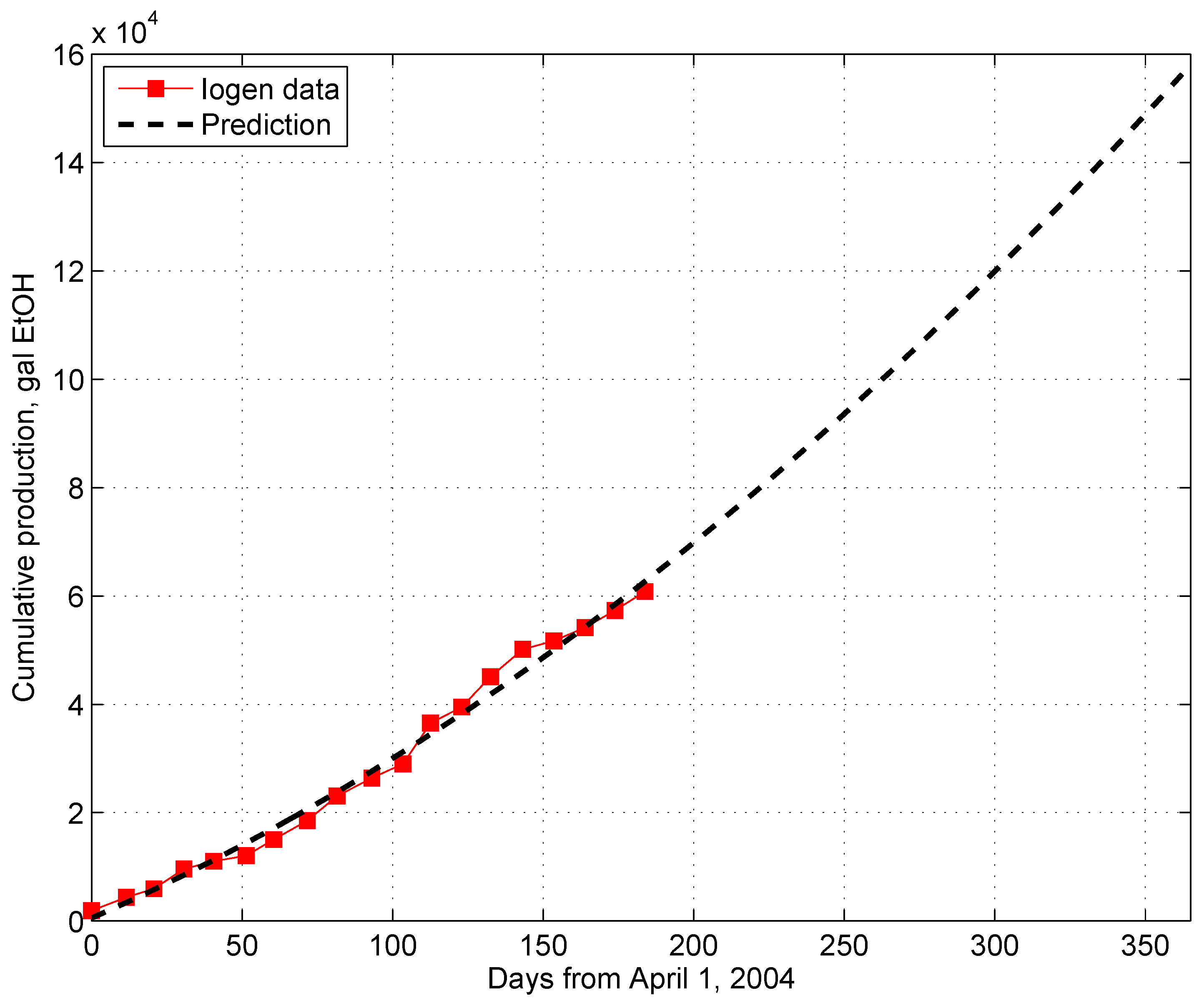
Wheat, oat, and barley straw are first pretreated with sulfuric acid and steam. Iogen’s patented enzymes then break the cellulose and hemicelluloses down into six- and five-carbon sugars, which are later fermented and distilled into ethanol. Standard yeast does not ferment the 5-carbon sugars, so genetically modified, delicate and patented yeast strains are used. Iogen’s plant has nameplate capacity of 1 million gallons of ethanol per year. The only publicly presented history of cellulosic ethanol production is shown in Figure 9.
From Figure 9 and [49,50] the following can be deduced:
- 600,000 L/year = 158,000 gallons/year of anhydrous ethanol, or 10 bbl/day = 6.7 bbl of equivalent gasoline/day were actually produced.
- There exists 2 × 52,000=104,000 gallons of fermentation tank volume.
- The ratio of the annual volume of ethanol production and the tank volume is 1.5 gallons of ethanol per gallon of fermenter and per year.
I then assume 7-day batches + 2-day cleanups. Given the reported ethanol production and the assumed batch times, there is ca. 4% of alcohol in a batch of industrial wheat-straw broth, in contrast to 12 to 16% of ethanol in corn-ethanol refinery broths. Shorter batch times lead to an estimation of even less favorable process parameters.
Since wheat is the largest grain crop in Canada, I use its straw as a reference (the barley and oats straws are similar). On a water-free basis, wheat straw has 33% of cellulose, 23% of hemicelluloses, and 17% total lignin [51]. Other sources report 38%, 29%, and 15%, respectively, see [52] for a data compilation. These differences are not surprising, given experimental uncertainties and variable biomass composition. To calculate ethanol yield, I use the more favorable, second set of data. The respective conversion efficiencies, assumed after Badger [53], are listed in Table 5.
Table 5.
Yields of ethanol from cellulose and hemicellulose. Source: Badger [53].
| Step | Cellulose | Hemicellulose |
| Dry straw | 1 kg | 1 kg |
| Mass fraction | ||
| Enzymatic conversion efficiency | ||
| Ethanol stoichiometric yield | ||
| Fermentation efficiency | ||
| Ethanol Yield, kg | 0.111 | 0.067 |
The calculated ethanol yield, 0.18 kg/(kg straw) (0.23 L/kg), is somewhat less than a recently reported maximum ethanol yield of 0.24 kg/kg [54] achieved in 500 mL vessels, starting from 48.6% of cellulose. Simultaneous saccharification and fermentation yielded 0.17 kg/kg, see Table 5 in [54].
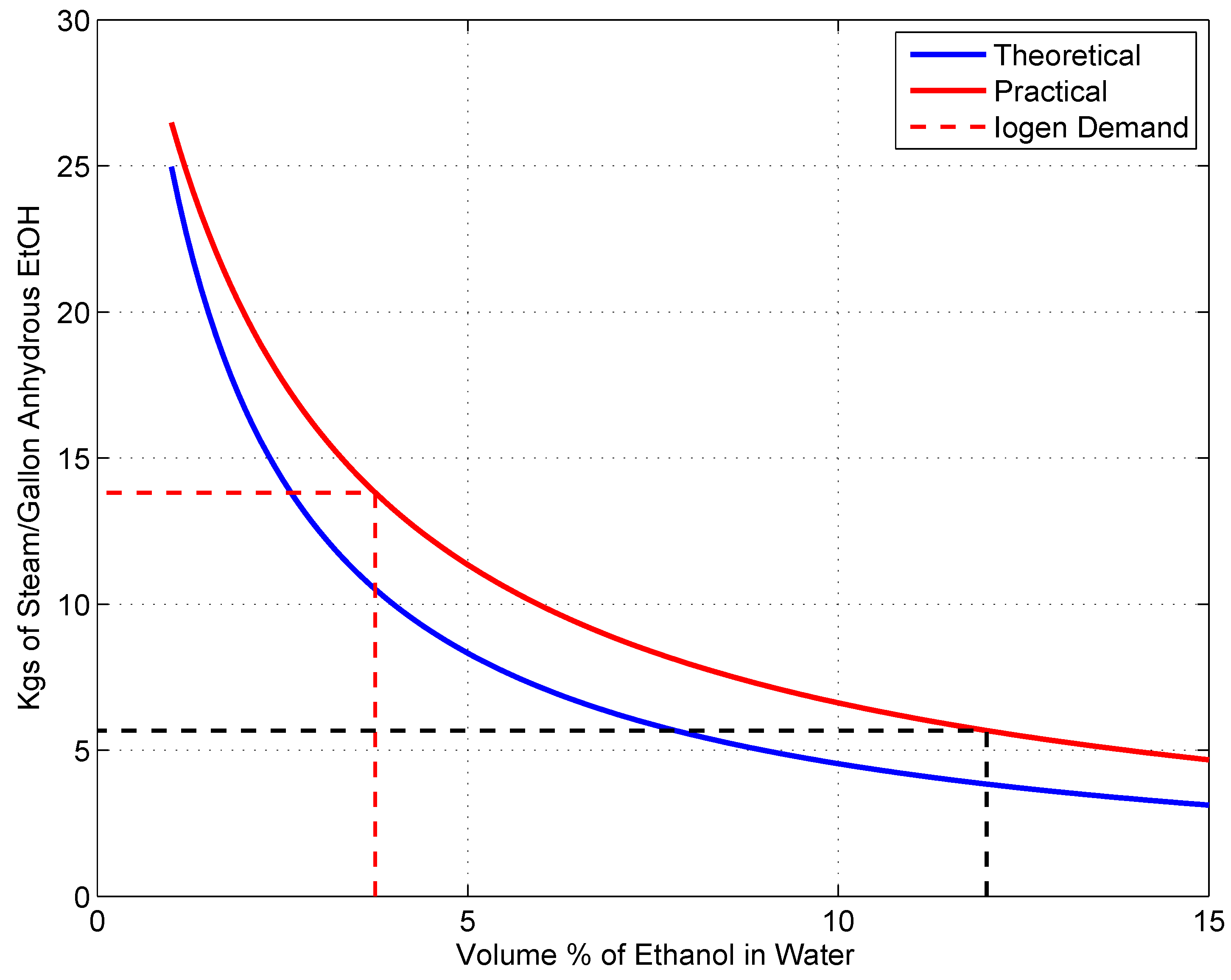
Because enzymatic decomposition of cellulose and hemicelluloses is inefficient, the resulting dilute broth requires 2.4 times more steam energy to distill than the average 15 MJL in an average ethanol refinery [28,29], see Figure 10.
One could argue that Iogen’s Ottawa facility is for demonstration purposes only and that the saccharification and fermentation batches were not regularly scheduled. Then, independently of Iogen’s data, an alternative calculation yields the same result: At about 0.2 to 0.25 kg of straw/L, the mash is barely pumpable. With Badger’s yield of 0.18 kg/kg, the highest ethanol yield is 3.5 to 4.4 % of ethanol in water.
The higher heating value (HHV) of ethanol is 29.6 MJ kg [29]. The HHV of wheat straw is 18.1 MJ kg [55] and that of lignin 21.2 MJ kg [56]. With these inputs, the first-law (energy) efficiency of Iogen’s facility is
where the density of ethanol is 0.787 kg L. The entire HHV of lignin is credited to offset distillation fuel, another optimistic assumption for the wet-separated lignin. Given expected moisture content, probably HHV of lignin should be used. Equation (2) also disregards the energy costs of steam treatments of the straw at 120 or 140 C, and the separated solids at 190 C, sulfuric acid and sodium hydroxide production, molecular sieves to reject the last 4 wt % of water from the azeotrope, etc.
The complex enzyme production processes also use plenty of energy. Since these processes are proprietary, only enzyme prices can be used as proxies for production complexity. The enzymes necessary to split cellulose fibers and chop them into small pieces are complex proteins [57] that need to be replicated on mass scale. Many tons of enzymes would have to be produced each year at a dose cost commensurate with ethanol that costs roughly 1 dollar per kilogram. These enzymes biodegrade, stick to the plant mash and are washed away, and must be replaced after each batch. Compare the low-cost requirement for the cellulose-splitting enzymes with an enzyme most commonly used in polymerase chain reactions (PCR). A DNA polymerase is an enzyme that assists in DNA replication. Such enzymes catalyze the polymerization of deoxyribonucleotides alongside a DNA strand, which they “read” and use as a template. The newly-polymerized molecule is complementary to the template strand and identical to the template’s partner strand. A common type of this enzyme is Taq DNA Polymerase from Thermus aquaticus, and its April 2010 price was between $300,000 and $1.2 million per kg, see Sigma Aldrich, www.sigmaaldrich.com/catalog/search/ProductDetail/SIGMA/D1806, accessed April 19, 2010. According to Genentech, the pharmaceutical proteins produced in bioreactors identical to those that might be used to produce the cellulose decomposition enzymes sell for up to $12 million per kg [58].
Figure 9.
Ethanol production in Iogen’s Ottawa plant [49]. Extrapolation to one year yields 158,000 gallons. Note that the data points are evenly spaced as they should be for regularly scheduled batches.
Figure 9.
Ethanol production in Iogen’s Ottawa plant [49]. Extrapolation to one year yields 158,000 gallons. Note that the data points are evenly spaced as they should be for regularly scheduled batches.

4. Calculation Methodology
4.1. Monte Carlo Simulations
Monte Carlo methods are a class of computational algorithms that rely on repeated random sampling of inputs to compute outcomes that are often represented in terms of their probability distribution functions and cumulative probability distributions. Monte Carlo simulations are useful in modeling systems with significant uncertainty in inputs, as in predicting expected ethanol yield from the geographically distributed switchgrass plantations. When Monte Carlo simulations were applied in space exploration and oil exploration, actual observations of failures, cost overruns and schedule overruns were routinely better predicted by the simulations than by human intuition or alternative “soft” methods [60].
Casler and Boe [19] conclude their paper as follows: “Biomass yield of switchgrass is unstable, varying by harvest date, site, year, and cultivar. Interactions among these factors cause biomass yield to be relatively unpredictable, particularly with respect to harvest date. For single harvest of switchgrass, aimed at bioenergy feedstock production, the optimal harvest date was in late summer or early autumn, when soil and air temperatures are sufficiently low to minimize the potential for regrowth. In the short term, an earlier harvest date could increase biomass yields, but this would have detrimental long-term effects on stands. In the long term, plant mortality is apparently reduced by delayed harvest and preservation of carbohydrate reserves.”
Figure 10.
Steam requirement in ethanol broth distillation. A 3.7% broth requires 2.4 times more steam than a 12% broth [59].
Figure 10.
Steam requirement in ethanol broth distillation. A 3.7% broth requires 2.4 times more steam than a 12% broth [59].

Fike et al. [38] state: “Limited information is available regarding biomass production potential of long-term (-yr-old) switchgrass. ...Yields at Site B (19.1Mgha) were about 35% greater than those at Site A (14.1Mgha), although the sites were only 200m apart.”
Therefore there is a need to capture the temporal and spatial variability of switchgrass yields in a statistical manner. This is done with a Monte Carlo procedure described next.
4.2. Distribution of Switchgrass Yields
We are interested in the most probable continuous biomass yield from any field, growing any switchgrass cultivar, geographically located in any state, harvested during any calendar year, and harvested after any number of years from seeding. Therefore all available field data are thrown into a single “data pool.” These data are then used to construct an empirical probability distribution function (pdf) and its integral, the cumulative distribution function (cdf) of switchgrass yields.
The purpose of pooling the switchgrass yield data was made clear in the discussion of switchgrass area required to power cars in a single metropolitan area. Since potentially tens of millions of acres of giant switchgrass monocultures will be needed, switchgrass will have to be grown in different geographical locations, perhaps even outside of the U.S., and on the contiguous fields similar in size to the giant sugarcane plantations in Brazil in the state of São Paulo.
The switchgrass yields were made dimensionless by dividing the data by 1 Mg ha y. The same procedure was applied in the derivation of all probability distribution functions and cumulative distribution functions in this paper.
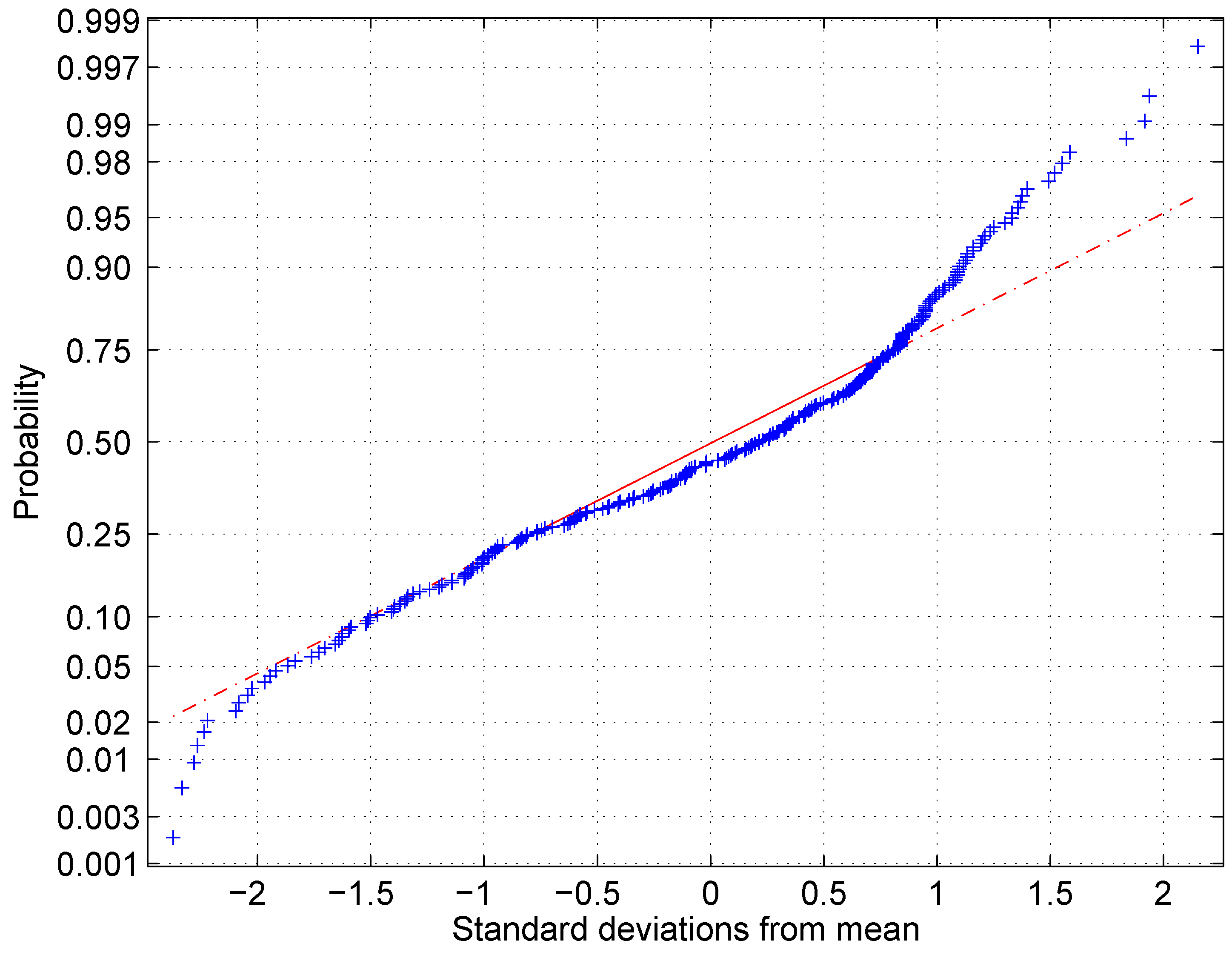
Figure 11.
The logarithm of the switchgrass yield data in [18,19,20,21,37] is approximately normally distributed. The underlying lognormal distribution has the mean Mg ha y, and the standard deviation Mg ha y.

The logarithm of the switchgrass yields shown in Figure 2, Figure 3, Figure 4, Figure 5, Figure 6 and Figure 7 is normally distributed,
with the mean and the standard deviation , see Figure 11. The lognormal mean is Mg ha yr, above the Schmer at al. mean of 7.2 Mg ha yr, and the standard deviation is Mg ha y.
To perform the Monte Carlo simulations of the switchgrass-ethanol cycle, random values are sampled from distribution Equation (3). The result is a random variable with a certain probability distribution function.
As discussed in the Switchgrass Yield section, the measured switchgrass yields often decline after 2-5 years, and none have been reported beyond 10 years. To translate from the reported annual switchgrass yields to the equivalent continuous yields, the following optimistic procedure is used. Let denote the minimum of , and its maximum. The weight function
accounts for the fact that higher yields are always associated with lower plant mortality [20]. The maximum age of surviving commercial switchgrass plants is assumed to be 20 years, the minimum age 5 years, and there is a 2-year grass establishment period with no harvest for the low-yield fields and a 1-year period for the high-yield ones. The continuous switchgrass yield is then given by the following random variable:
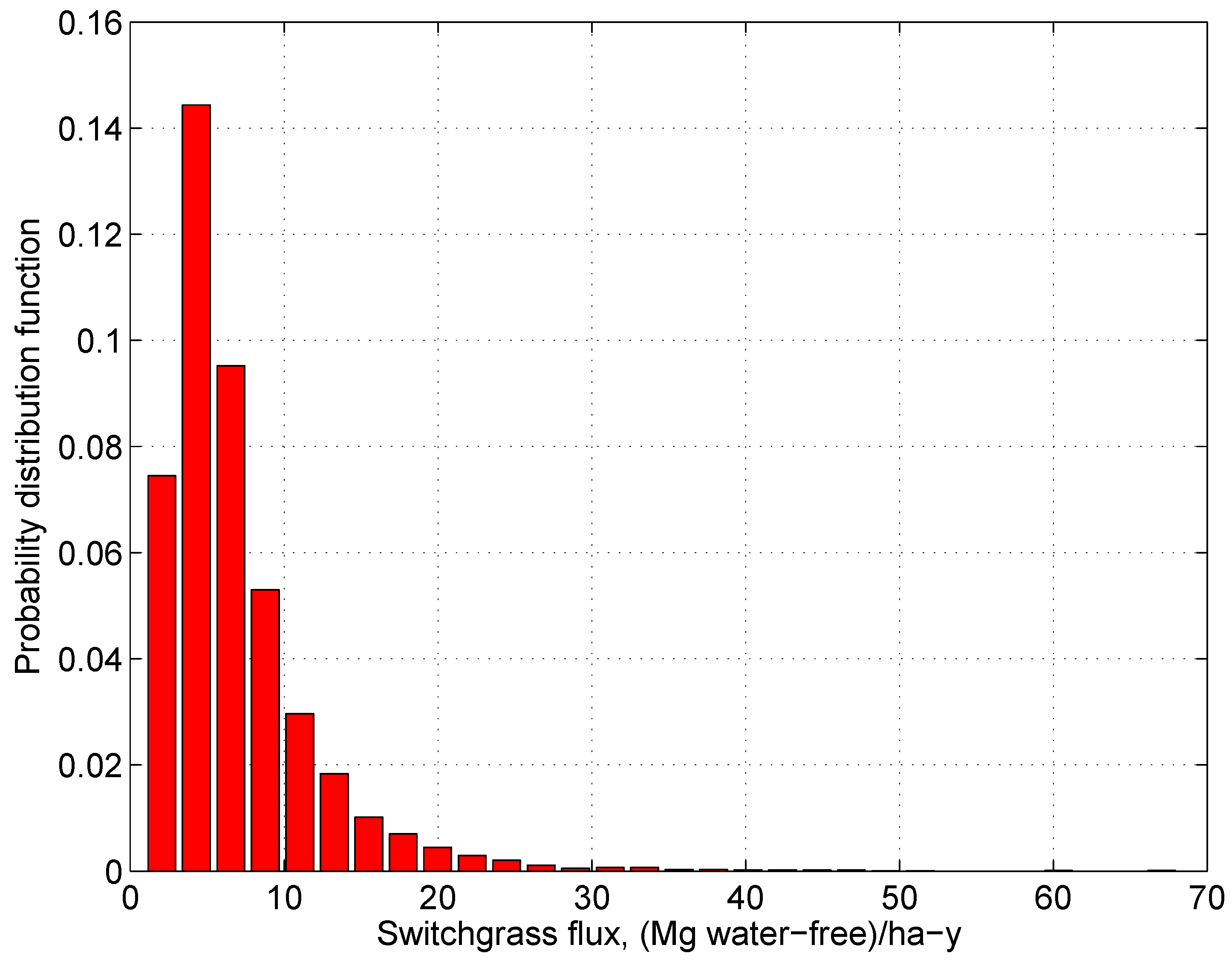
where ⊗ denotes the element-by-element multiplication of the two random variables. The mean of the “continuous yield” distribution (5) is Mg ha y, slightly lower than that of Schmer et al., and its standard deviation is Mg ha y. Its probability distribution function is shown in Figure 12. Reviewer A should not defend the analysis by Schmer et al., while at the same time criticizing the analysis here: Both means are comparable, but this analysis gives the full context of the mean.
Figure 12.
The probability distribution function (pdf) of the continuous mass flux of switchgrass (“continuous yield”). The mean is Mg ha y, and the standard deviation Mg ha y.
Figure 12.
The probability distribution function (pdf) of the continuous mass flux of switchgrass (“continuous yield”). The mean is Mg ha y, and the standard deviation Mg ha y.

4.3. A Prototype of the Switchgrass-Based Ethanol Refinery
Mass Balance
The composition of switchgrass in the south-central U.S. has been evaluated by Cassida et al. [61]. The cellulose content varies from 34 to 46% by mass with the mean of 39%. The lignin content varies from 7 to 12% with the mean of 9%. The hemicellulose content is not reported. Lee et al. [52] list 37% of cellulose, 29% of hemicelluloses, and 19% of lignin on the average. I use the latter, more favorable estimate in my calculations, and the yield of switchgrass ethanol is almost identical to that calculated in Table 5 for wheat straw.
The cellulose weight fraction is assumed to be normally distributed after [46]. The mean, maximum, and minimum measured values are taken from [61]. The mean is , and the standard deviation is . The normally distributed random mass fractions of cellulose are . It is assumed that the mass fraction of hemicelluloses varies in proportion to that of cellulose:
and, from the mass balance, the lignin mass fraction is
Refinery Efficiency
The most-often quoted yield of ethanol from switchgrass, 0.38 L/kg (90% of the theoretical yield), is based on the Berkeley Energy and Resources Group’s Biofuel Analysis Meta-Model (EBAMM) [24,25], and has no justification—whatsoever—in the context of chemistry relevant to this analysis. In Section 3.4, I have used the published fragments of industrial data [49,50] to arrive at a realistic efficiency of a “cellulosic ethanol” refinery of 0.23 L/kg. The ethanol yield, 0.18 kg EtOH(kg switchgrass), calculated here, is equivalent to L/kg of switchgrass, infinitesimally lower that the 0.24 L/kg reported by Lau and Dale [47], but significantly lower than the 0.28 L/kg claimed in [62], or the 0.38 L/kg asserted in EBAMM.
For the lignin content between 9 and 19%, the range of energy efficiencies of a switchgrass “cellulosic ethanol” refinery is 20–24% if the burned lignin is bone dry and no other energy costs are incurred. With one significant digit we get ca. 20% from Equation (2). At this efficiency, roughly 5 units of heat from switchgrass are necessary to obtain 1 unit of heat from 100% ethanol. The higher heating value of switchgrass is 18.1 MJ kg [63]. Therefore, it takes kg of switchgrass to obtain 1 kg of anhydrous ethanol, or 6.5 kg of switchgrass to obtain 1 L of the ethanol.
If the entire process of ethanol production is driven by burning lignin from fermented switchgrass, as well as burning additional bone dry switchgrass, the average yield of ethanol is between L ha y and 11,000/6.5 ≈ 1,700 Lhay for the data in Figure 2, Figure 3, Figure 4, Figure 5, Figure 6 and Figure 7.
The ethanol yield used in the Monte Carlo simulations here is assumed after Badger, see Table 5, with the switchgrass composition calculated from Equations (6)–(7). The resulting pdf is shown in Figure 13. The energy efficiency of a switchgrass refinery, η (energy out as anhydrous ethanol divided by net energy in from switchgrass), is calculated from Equation (2), with the random lignin mass fraction given by Equation (7), and the random ethanol yield sampled from the distribution in Figure 13. The resulting pdf is shown in Figure 14.
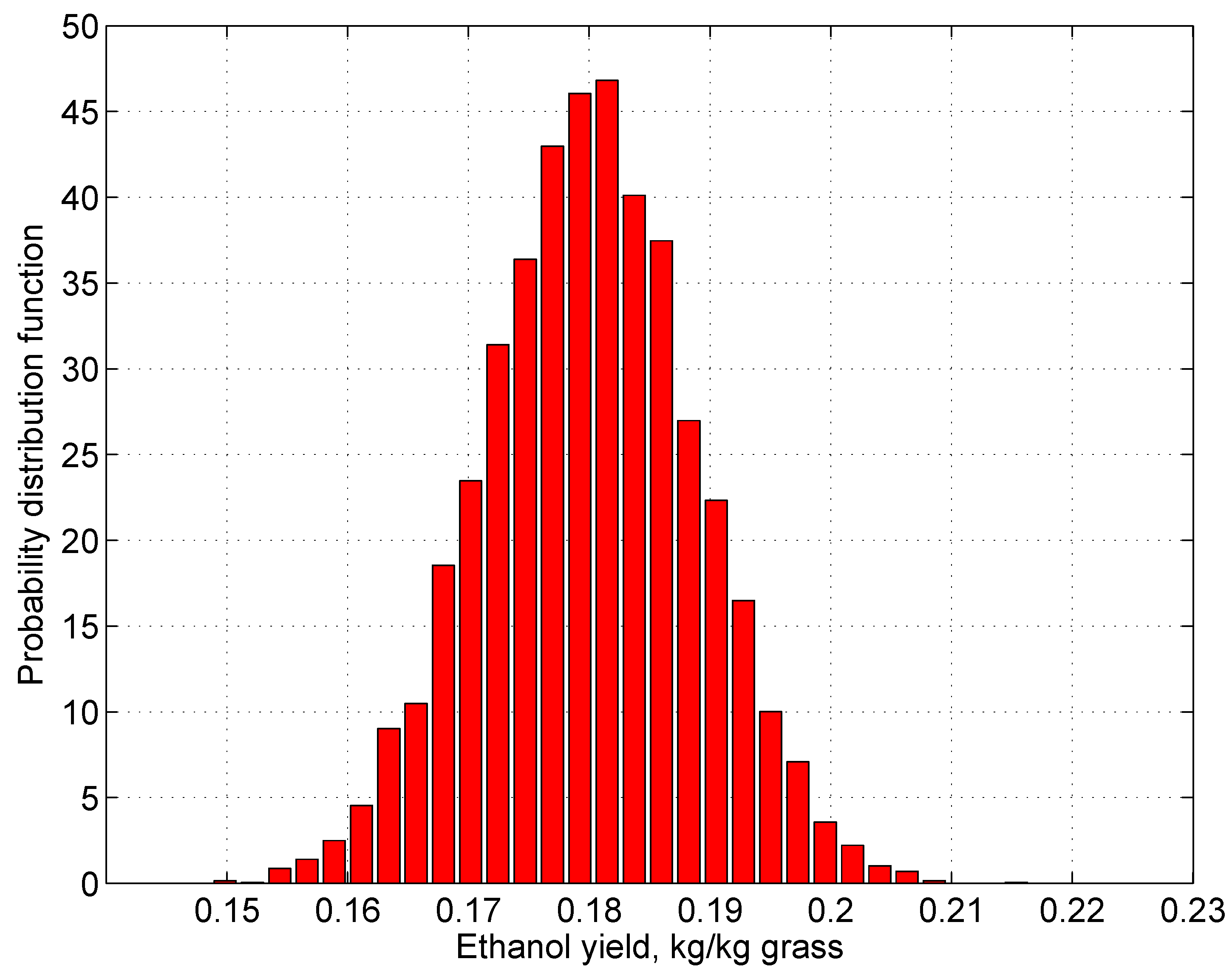
Figure 13.
The probability distribution function (pdf) of ethanol yield from switchgrass. The mean is kg kg, and the standard deviation kg kg.
Figure 13.
The probability distribution function (pdf) of ethanol yield from switchgrass. The mean is kg kg, and the standard deviation kg kg.

Figure 14.
The probability distribution function (pdf) of energy efficiency, η, of a switchgrass ethanol refinery. The mean is MJ/MJ, and the standard deviation MJ/MJ.
Figure 14.
The probability distribution function (pdf) of energy efficiency, η, of a switchgrass ethanol refinery. The mean is MJ/MJ, and the standard deviation MJ/MJ.

5. Results
5.1. Effective Volumetric Flux of Ethanol
The effective volumetric flux of ethanol from the switchgrass field/switchgrass-powered ethanol refinery cycle (“ethanol yield”) is calculated as
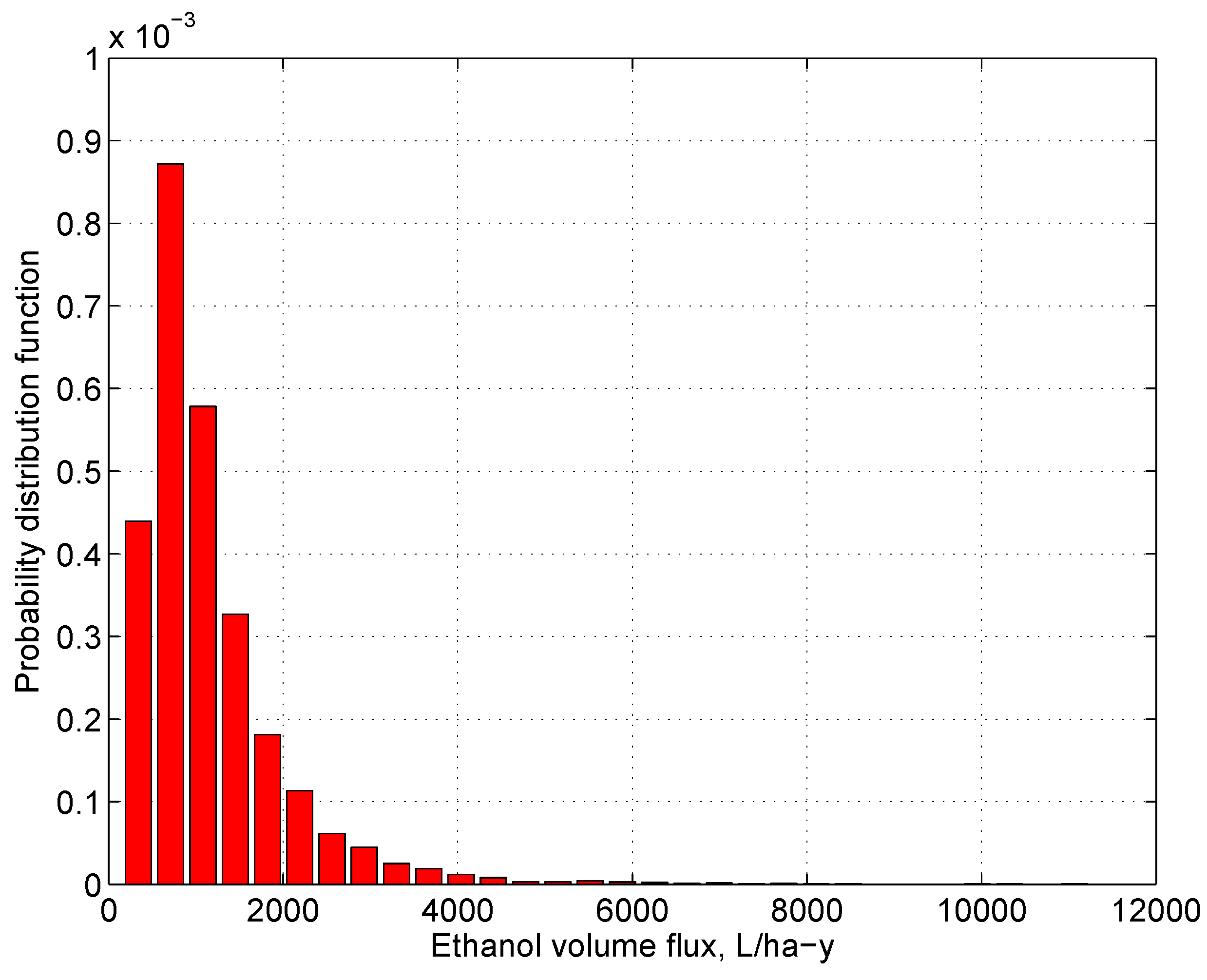
and the resulting pdf is shown in Figure 15. Note that the lognormal mean, L ha y and its standard deviation L ha y, are in the range estimated for the data in Figure 2, Figure 3, Figure 4, Figure 5, Figure 6 and Figure 7, 650–1,700 L ha y. The most probable values of ethanol yield are clustered about the lognormal mean in the bin 817–1,270 L ha y. When the lognormal mean of the continuous harvest of switchgrass, 6.83 Mg ha y, is multiplied by the mean refinery yield, 0.23 L/kg, the result is 1,570 L ha y.
Remark:
It should be stressed that a simple multiplication of means of different probability distributions, a standard procedure in most biofuel papers, does not yield the most probable value of the switchgrass ethanol yield.
5.2. Probability of Exceeding a Given Flux
By integrating the pdf functions in Figure 12 and Figure 15, one may estimate the probabilities of exceeding a given value of flux. The probability of achieving a continuous mass flux of switchgrass larger than the abscissa is plotted in Figure 16. The probability of achieving a net ethanol fuel yield (after satisfying the refinery energy needs) larger than the abscissa is plotted in Figure 17.
5.3. Summary of Results Thus Far
The continuous mean switchgrass yield based on Figure 2, Figure 3, Figure 4, Figure 5, Figure 6 and Figure 7 has the expected value of Mg ha y, see Figure 12, close to 7.2 Mg ha y estimated in [21], but sharply lower than 25.8 Mg ha y claimed elsewhere [64,65]. If switchgrass is used as the refinery fuel, the most probable ethanol yield is about 1100 L ha y. The probability of ethanol yields in the range 1200–1700 L ha y is sharply less than 0.5.
Figure 15.
The probability distribution function (pdf) of the effective volumetric ethanol flux. The lognormal mean is L ha y. The standard deviation, L ha y, is comparable to the mean, indicating a long tail of the highly improbable large fluxes.
Figure 15.
The probability distribution function (pdf) of the effective volumetric ethanol flux. The lognormal mean is L ha y. The standard deviation, L ha y, is comparable to the mean, indicating a long tail of the highly improbable large fluxes.

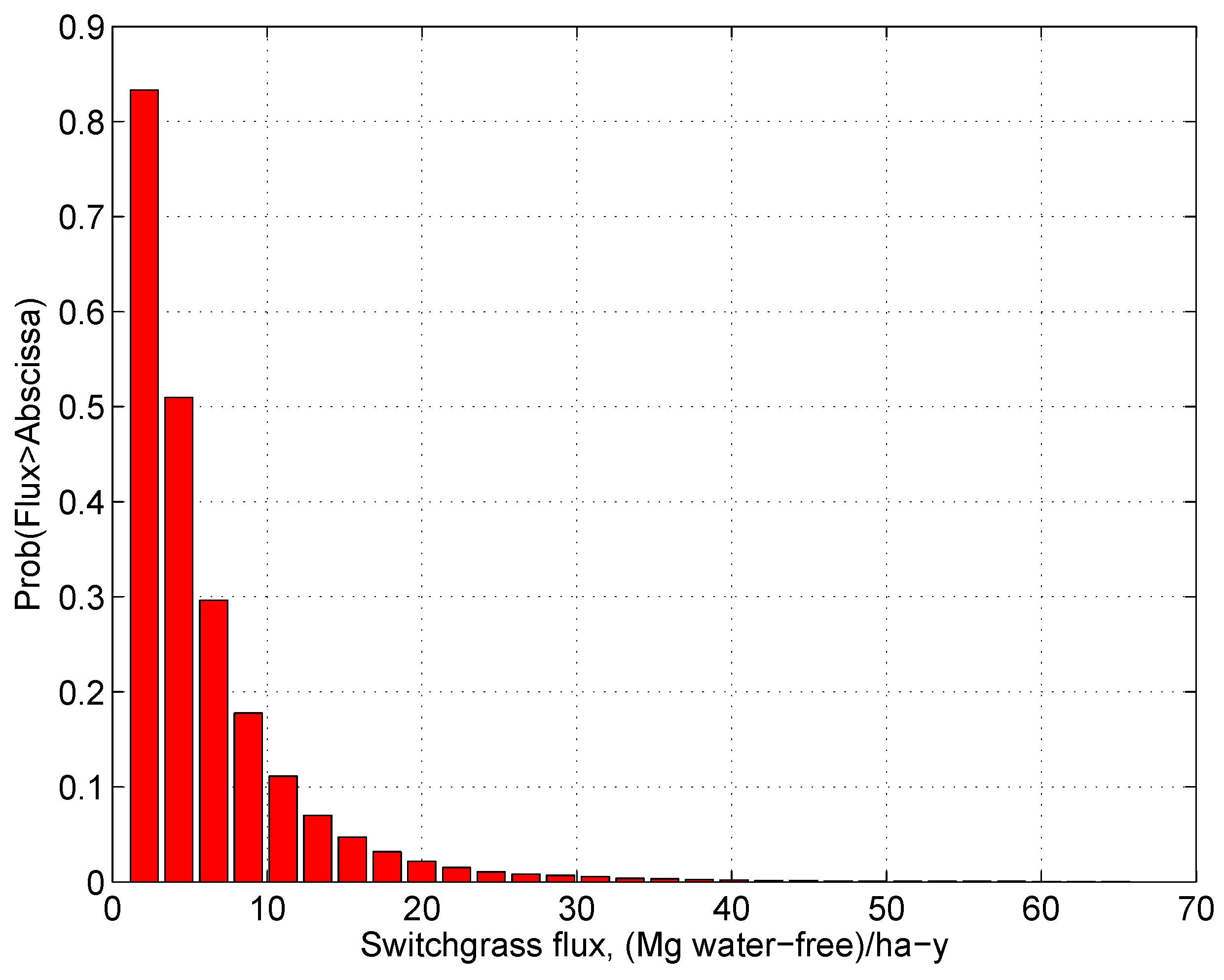
Figure 16.
Probability that a continuous switchgrass mass flux (“continuous yield”) exceeds a given value. If the abscissa is , the ordinate is derived from the yield data in [18,19,20,21,37,38,39], weighted by the switchgrass survivability function defined in Equation (4).

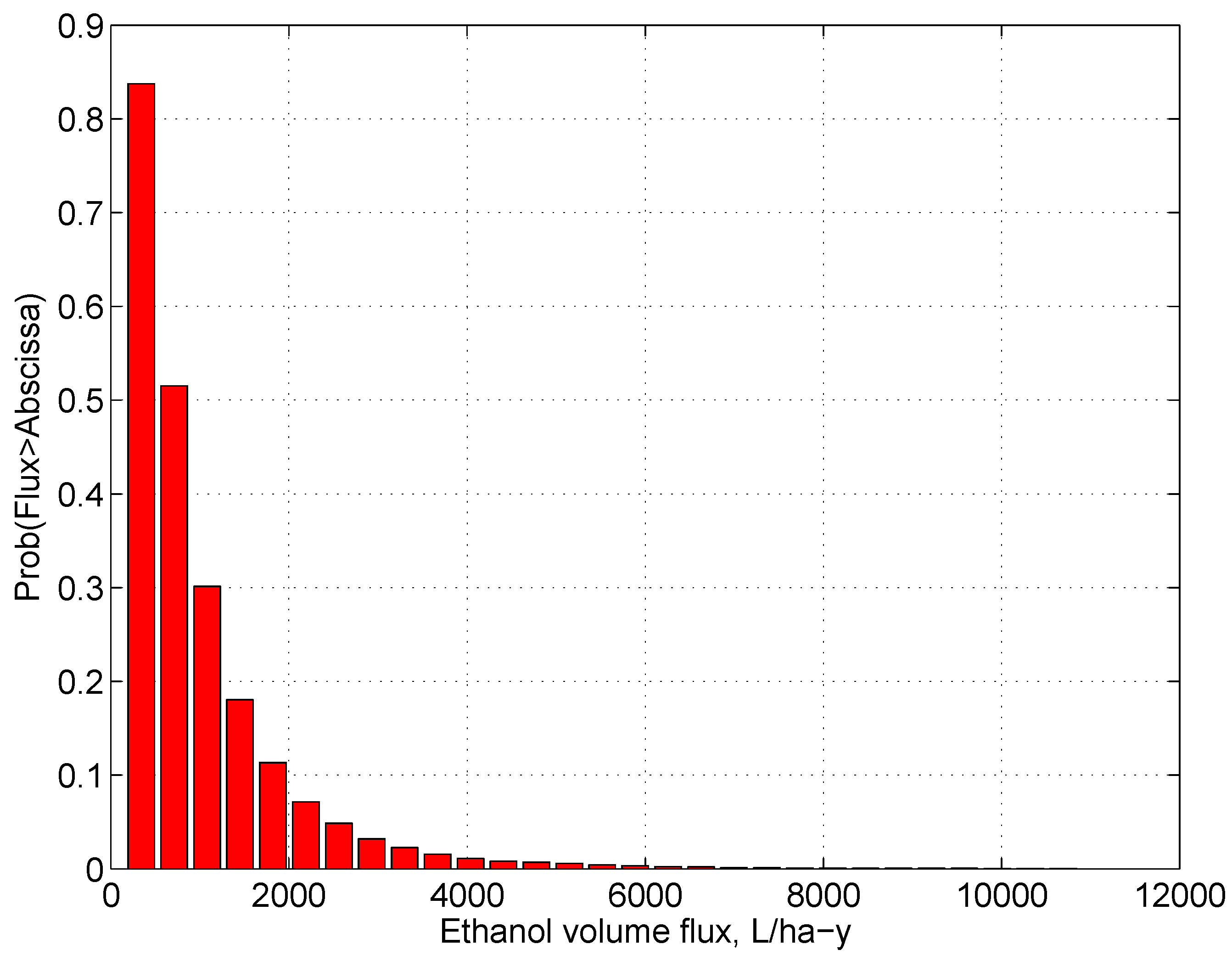
Figure 17.
Probability that a continuous volumetric flux of ethanol exceeds a given value. If the abscissa is , the ordinate is derived from Figure 16 and the refinery efficiency calculated in Section 3.4
Figure 17.
Probability that a continuous volumetric flux of ethanol exceeds a given value. If the abscissa is , the ordinate is derived from Figure 16 and the refinery efficiency calculated in Section 3.4

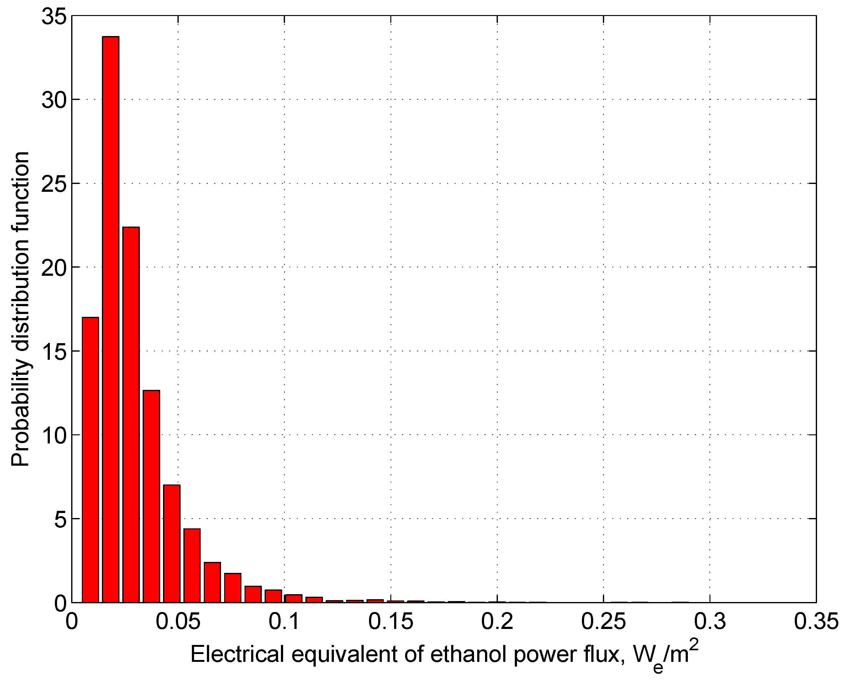
Figure 18.
The probability distribution function (pdf) of the continuous electrical power flux generated from the switchgrass-ethanol cycle.
Figure 18.
The probability distribution function (pdf) of the continuous electrical power flux generated from the switchgrass-ethanol cycle.

5.4. Continuous Electrical Power from Switchgrass Ethanol
Photovoltaic (PV) solar cells generate electricity that can be converted to power a rotating shaft with almost 100% efficiency. The following formula converts the volumetric flux of ethanol from the switchgrass-ethanol cycle discussed here to continuous electrical power:
where is the average efficiency of converting ethanol to electricity. Here .
The pdf and the exceedance probability function of continuous electrical power generated from the switchgrass-ethanol cycle are shown in Figure 18 and Figure 19.
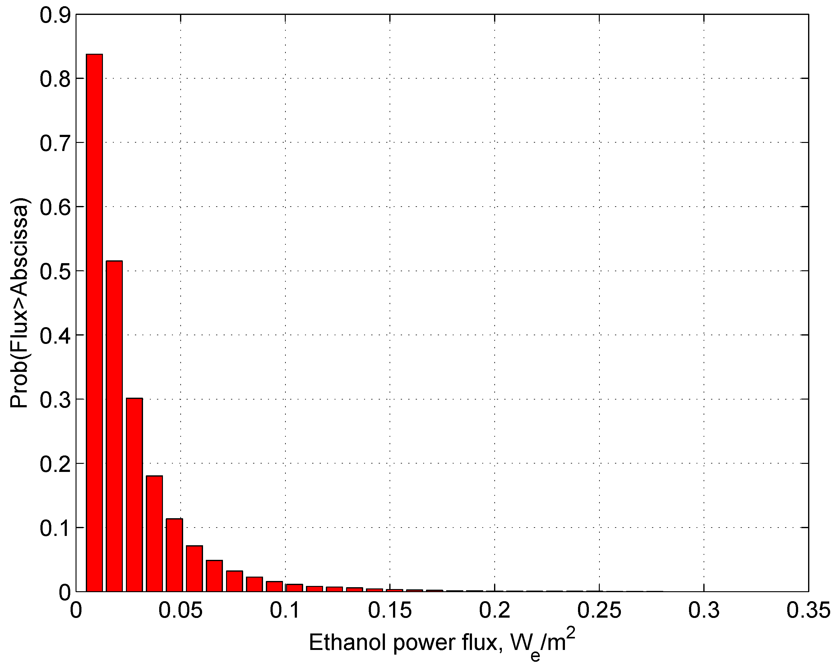
Figure 19.
Probability that a continuous electrical power flux of ethanol generated from switchgrass exceeds a given value. If the abscissa is , the ordinate is derived from Figure 18.
Figure 19.
Probability that a continuous electrical power flux of ethanol generated from switchgrass exceeds a given value. If the abscissa is , the ordinate is derived from Figure 18.

The probability of generating more than 0.03 W/m continuously is less than 50%. Note that only the electrical power inputs are compared here. The substantial continuous energy inputs to switchgrass and switchgrass ethanol, as well to initial energy inputs to PV cells are not discussed here. For more detailed approaches see [16,30,66].
On average, switchgrass ethanol delivers 0.03 W per m of field surface (1 W is one watt of electrical power). Also on average, a mediocre, see Figure 20, 10%-efficient PV cell that uses twice the area of panels for access roads, etc., delivers × 200 × W/m continuously when it operates anywhere in the U.S. [16,30]. A better PV panel could deliver 40 W/m continuously. Thus our present mediocre PV panel is 335 times more efficient than the switchgrass-ethanol cycle in delivering continuous power of a rotating shaft. In other words, on the average, 1 hectare (10,000 m or 2.5 acres) of switchgrass field is equivalent to 30 m of the spread out and inefficient PV cells. An efficient—currently available—PV cell takes a 4-by-4 meter area, see Figure 21, and costs about 16,000 March 2008 U.S. dollars to install on a house roof. It is designed to run for 30 years with almost no maintenance.
Figure 20.
Solar light conversion efficiencies of best research photovoltaic cells. Source: Lawrence Kazmerski, Don Gwinner, Al Hicks, NREL, 11/11/07, www.nrel.gov/- pv/thin_film/docs/kaz_best_research_cells.ppt.
Figure 20.
Solar light conversion efficiencies of best research photovoltaic cells. Source: Lawrence Kazmerski, Don Gwinner, Al Hicks, NREL, 11/11/07, www.nrel.gov/- pv/thin_film/docs/kaz_best_research_cells.ppt.

6. Equivalent CO Emissions
The procedure of calculating equivalent CO emissions is explained in [29], Section 5.1 and Table 19. The CO emissions from the oxidation of soil humus are described in [28], p. 267. Only updates or parameter changes are discussed here.
6.1. NO emissions from agriculture
As stated by Crutzen et al. [67]: “An evaluation of hundreds of field measurements has shown that N fertilization causes a release of NO in agricultural fields that is highly variable but averages close to 1% of the fixed nitrogen input from mineral fertilizer or biologically fixed N [68,69], and a value of 1% for such direct emissions has recently been adopted by [70]. There is an additional emission from agricultural soils of 1 kg NO–N ha y, which does not appear to be directly related to recent fixed N-input. The in-situ fertilizer-related contribution from agricultural fields to the NO flux is thus 3–5 times smaller than our adopted global average NO yield of % of the fixed N input. The large difference between the low yield of NO in agricultural fields, compared to the much larger average value derived from the global NO budget, implies considerable “background” NO production occurring beyond agricultural fields, but, nevertheless, related to fertilizer use, from sources such as rivers, estuaries and coastal zones, animal husbandry and the atmospheric deposition of ammonia and NO.” Fortunately, my old calculation [29] of the total emissions from ammonium nitrate was 4.4%, significantly larger than the IPCC estimates. At the time, I was criticized for this calculation as exaggerated and unrealistic. Here I continue to use my old estimate, now verified independently by Crutzen et al. The smaller GHG emissions for urea production are accounted for in the current analysis.
Figure 21.
30 m of panel and road area are necessary to generate the same electrical power from the inefficient PV cells (dark grey) as from 1 ha of average switchgrass field dedicated to producing ethanol (light grey). The barely visible 15 m of a current efficient PV panel are in white.
Figure 21.
30 m of panel and road area are necessary to generate the same electrical power from the inefficient PV cells (dark grey) as from 1 ha of average switchgrass field dedicated to producing ethanol (light grey). The barely visible 15 m of a current efficient PV panel are in white.

6.2. CO emissions from lime
6.3. Soil erosion rate
The average soil erosion rate for switchgrass is assumed to be 3 Mg ha y or 25% of the ca. 13 Mg ha y of the erosion rate typical of corn agriculture in recent times. (Source: United States Department of Agriculture, National Resources Conservation Service. The reported erosion rate is the sum of water and wind erosion rates from Tables 10 and 11 at www.nrcs.usda.gov/technical/agronomy.html, see also Figures 9–11 in [31].)
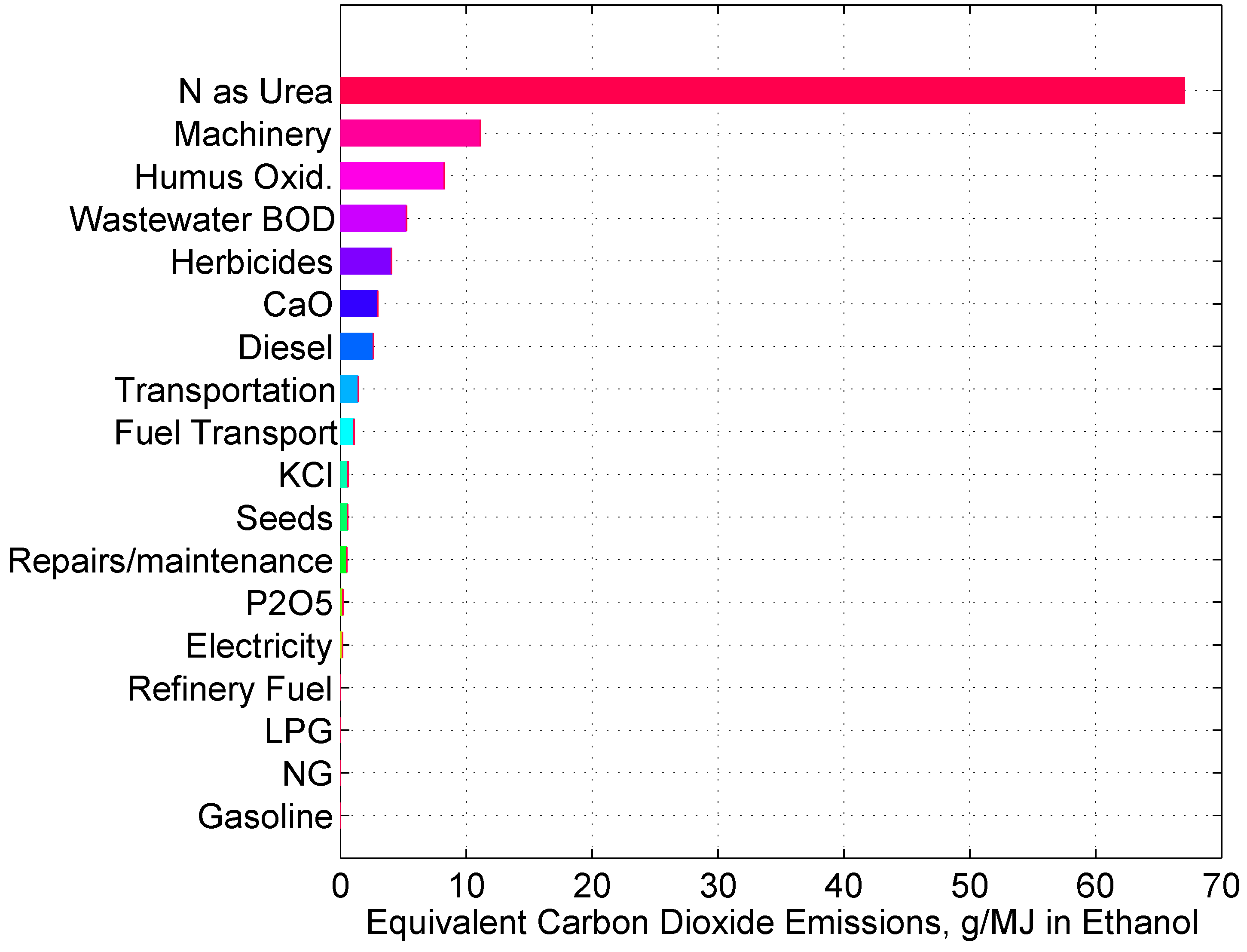
Figure 22.
Equivalent CO emissions from the switchgrass-ethanol cycle.

6.4. Emissions from the refinery
As switchgrass is burned in the refinery to provide process heat and electricity, only emissions from the ethanol and denaturant transportation are included, as well as emissions from wastewater cleanup. The calculation results are shown in Figure 22 for the ethanol yield equal to the lognormal mean L ha y. The total emissions are dominated by the emissions from nitrogen fertilizer production and agricultural emissions from its application.
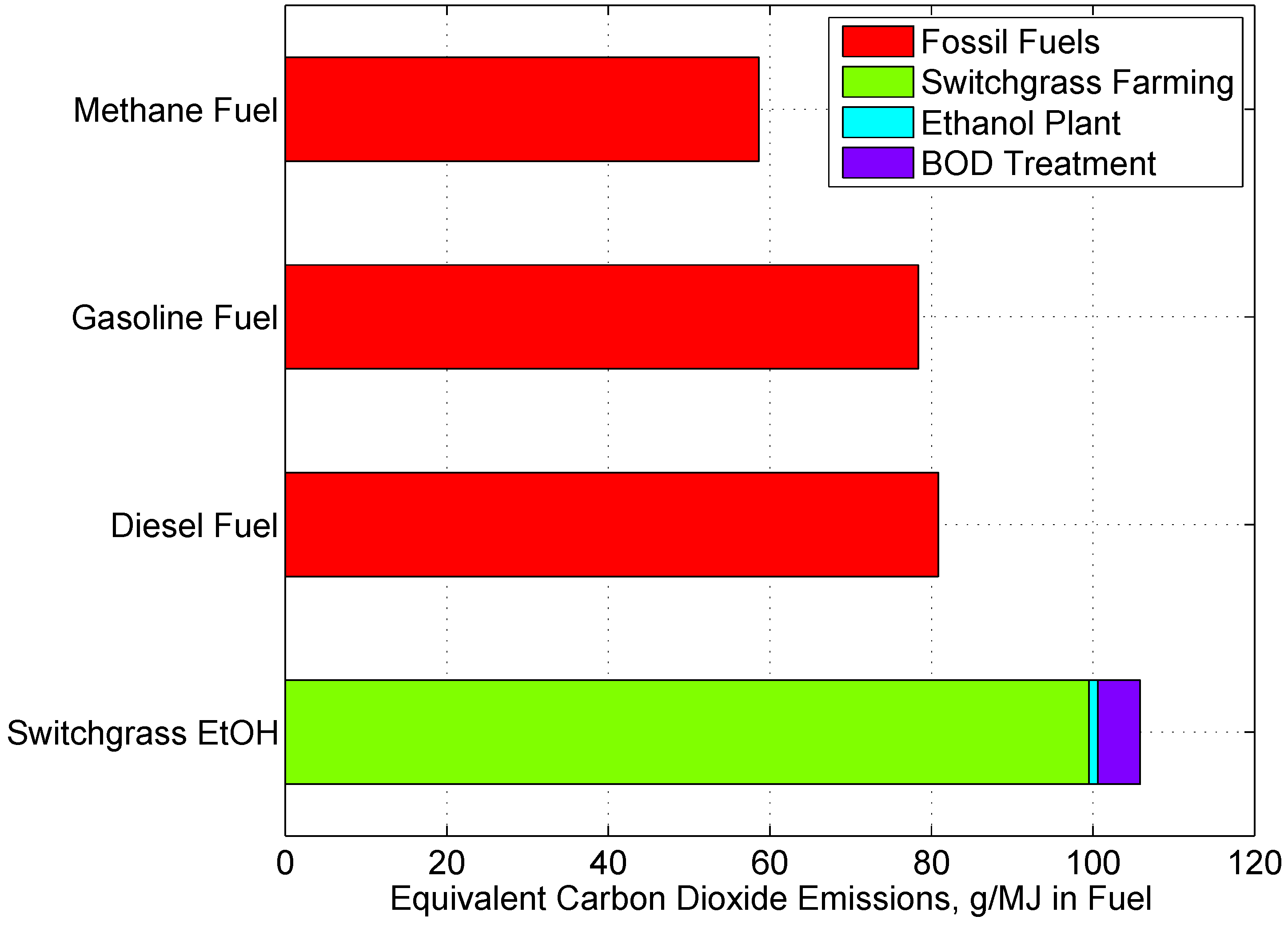
Using the lognormal mean of ethanol yield, L ha y, cumulative greenhouse gas (GHG) emissions are 106 g CO equiv./MJ in the anhydrous ethanol (1 MJ = joules). The GHG emissions from switchgrass ethanol are 35% higher than those from producing and burning automotive gasoline outright, see Figure 23, and two times higher than those from producing and burning compressed natural gas. The GHG emissions from switchgrass ethanol are generated only by the non-renewable resources consumed in its production, and by the NO/NO emissions from switchgrass agriculture. If one were to replace 10% of the current gasoline consumption in the U.S. with switchgrass ethanol, about 55 million tons of equivalent CO would be generated each year over and above the displaced gasoline emissions. Compressed natural gas is by far the most environmentally-friendly automotive fuel and its expansion should be considered urgently [71]. Corn ethanol agriculture generates GHG emissions of about 120 g/MJ in anhydrous ethanol, see Figure 8 in [28]. Therefore, replacing corn fields with switchgrass fields will result on the average in a reduction in net GHG emissions. In both cases, no land-use changes were included in the calculations.
Figure 23.
Specific greenhouse gas emissions from compressed methane, gasoline, diesel fuel, and switchgrass ethanol. Note that the non-renewable resources consumed to produce the ethanol generate 35% more emissions than gasoline and 2x those from methane.
Figure 23.
Specific greenhouse gas emissions from compressed methane, gasoline, diesel fuel, and switchgrass ethanol. Note that the non-renewable resources consumed to produce the ethanol generate 35% more emissions than gasoline and 2x those from methane.

A word of caution is in order. Net GHG emissions from the switchgrass ethanol cycle depend very strongly on the cycle’s yield. If, for example, 1,600 L ha y were produced, the net emissions of switchgrass ethanol would be zero relative to those of the displaced gasoline; compressed natural gas would still generate 25% fewer emissions.
7. Summary and Conclusions
In mid-2010, all published analyses of the switchgrass-ethanol cycle were work in progress, because of the still insufficient knowledge of the system. The main strength of the approach presented in this paper is in showing the context of the various measures of switchgrass field productivity and ethanol yields. The probability of achieving a continuous switchgrass yield of 8–10 Mg ha y is sharply less than 50%, see Figure 16. The probability of achieving a continuous ethanol yield of 1,200–1,600 L ha y is also sharply less than 50%, Figure 17. Achieving the 3,000–5,000 L ha y yields, asserted in the literature [21,62], is possible, but with a probability less than 0.05, in the noise of the current model.
Suppose that one would like to replace 18% of the current 20 EJ y the U.S. uses as automotive gasoline [16]. If the switchgrass ethanol cycle described here were used to achieve this goal with close to 50% probability, one would need at 140 million hectares of switchgrass, or the entire area of active U.S. cropland, using the mean of the energy efficiency distribution in Figure 17. The U.S. agricultural area is from www.ers.usda.gov/AmberWaves/July06SpecialIssue/pdf/BehindDataJuly06.pdf. According to USDA, the total U.S. cropland area (harvested, summer fallow, and failed) was 140 million hectares in 2006. Another 40 million hectares were devoted to pastures and idle cropland.
With the existing fermentation processes and technology, one obtains 0.23 L EtOH/kg of switchgrass, rather than 0.38 L/kg asserted in EBAMM. The relative difference is 37%. Because the overall energy efficiency of a plausible switchgrass ethanol refinery is only 20%, 6.5 kg of switchgrass must be processed and/or burned to obtain 1 L of the ethanol. This requirement translates into an optimistic most probable continuous yield of ethanol of about 1,100 L EtOH ha y, if switchgrass is used to power the refineries.
The law of energy conservation requires that a switchgrass ethanol refinery has a highly negative difference of output energy—input energy, or net-energy value (NEV), as shown previously in [27]. This statement follows directly from the observation that the switchgrass-ethanol process has a low energy efficiency and requires large external inputs of energy-intensive chemicals, heat, and electricity. Whether or not nonrenewable energy is used for biorefinery energy needs, .
The industrial switchgrass plantations considered here are sun-driven, man-made “machines,” whose ultimate output is shaft work used for generation of electricity or rotation of car wheels. These vast and complex machines should be compared against two other, much simpler devices that also convert solar energy into shaft work: solar photovoltaic (PV) cells (and electricity from thermal solar) and wind turbines. PV cells (whenever their panel areas measured in km become commercially available) convert solar energy directly into electricity, the most valuable form of free energy, that can be further converted into mechanical work with small losses. Wind turbines produce electricity from the kinetic energy of the sun-driven wind, and are not discussed here. All biofuel-producing systems should be judged on their ability to generate shaft work, not merely a biofuel.
PV cell, thermal solar, and battery R&D, as well as a large-scale implementation of already existing PV cell manufacturing technologies, could have a much larger impact on both near- and long-term energy security of the U.S. and Europe than biofuels.
Acknowledgements
I would like to thank the four anonymous reviewers of this paper. In particular, Reviewer A provided 11 pages of an exquisitely negative assessment of the manuscript that considerably sharpened my arguments. Reviewer D provided on 7 pages a thoughtful, thorough and positive assessment, with 5 pages of suggestions for improvement that were all gratefully accepted.
References
- Taiz, L.; Zeiger, E. Plant Physiology, 2nd ed.; Sinauer Associates: Sunderland, MA, USA, 1998. [Google Scholar]
- Zeltich, I. Photosynthesis, Photorespiration, and Plant Productivity; Academic Press: New York, NY, USA, 1971. [Google Scholar]
- Schweiger, R.G. New Cellulose Sulfate Derivatives and Applications. Carbohydrate Res. 1979, 70, 185–198. [Google Scholar] [CrossRef]
- Fan, L.T.; Lee, Y.H.; Beardmore, D.H. Mechanism of the Enzymatic Hydrolysis of Cellulose: Effects of Major Structural Features of Cellulose on Enzymatic Hydrolysis. Biotechnol. Bioeng. 1980, XXII, 177–199. [Google Scholar] [CrossRef]
- San Martin, R.; Blanch, H.W.; Wilke, C.R.; Sciamanna, A.F. Production of Cellulase Enzymes and Hydrolysis of Steam-Exploded Wood. Biotechnol. Bioeng. 1986, XXVIII, 564–569. [Google Scholar] [CrossRef] [PubMed]
- Lynd, L.R.; Weimer, P.J.; van Zyl, W.; Pretorius, I. Microbial Cellulose Utilization: Fundamentals and Biotechnology. Microbiol. Mol. Biol. Rev. 2002, 66, 506–577. [Google Scholar] [CrossRef] [PubMed]
- Zhang, Y.; Lynd, L.R. Cellodextrin Preparation by Mixed-Acid Hydrolysis and Chromatographic Separation. Anal. Biochemistry 2003, 322, 225–232. [Google Scholar] [CrossRef]
- Zhang, Y.; Lynd, L.R. Towards an Aggregated Understanding of Enzymatic Hydrolysis of Cellulose: Noncomplexed Cellulase Systems". Biotechnol. Bioeng. 2004, 88, 797–824. [Google Scholar] [CrossRef] [PubMed]
- Lee, Y.H.; Fan, L.T. Kinetic Studies of Enzymatic Hydrolysis of Insoluble Cellulose: (II). Analysis of Extended Hydrolysis Times. Biotechnol. Bioeng. 1983, XXV, 939–966. [Google Scholar] [CrossRef] [PubMed]
- Fan, L.T.; Lee, Y.H. Kinetic Studies of Enzymatic Hydrolysis of Insoluble Cellulose: Derivation of a Mechanistic Kinetic Model. Biotechnol. Bioeng. 1983, XXV, 2707–2733. [Google Scholar] [CrossRef] [PubMed]
- Ayres, R.U.; Ayres, L.W.; Warr, B. Exergy, Power and Work in the U.S. Economy, 1900–1998; Center for the Management of Environmental Resources, 2002. Available online: http://www.iea.org/work/2004/eewp/Ayres-paper3.pdf (accessed on 20 September 2010).
- Perlack, R.D.; Wright, L.L.; Turhollow, A.F.; Graham, R.L.; Stokes, B.J.; Erbach, D.C. Biomass as Feedstock for a Bioenergy and Bioproducts Industry: The Technical Feasibility of a Billion-Ton Annual Supply. Joint Report, Prepared by U.S. Department of Energy, U.S. Department of Agriculture, Environmental Sciences Division, Oak Ridge National Laboratory, P.O. Box 2008, Oak Ridge, TN 37831-6285, USA, 2005. Managed by: UT-Battelle, LLC for the U.S. Department of Energy under contract DE-AC05-00OR22725 DOE/GO-102005-2135 ORNL/TM-2005/66.
- Somerville, C. The Billion-Ton Biofuels Vision—Editorial. Science 2006, 312, 1277. [Google Scholar] [CrossRef] [PubMed]
- Khosla, V. Biofuels: Think outside the Barrel. Available online: www.khoslaventures.com/- presentations/Biofuels.Apr2006.ppt, 2006; video.google.com/videoplay?docid=-57028888912895-0913 (accessed on 20 September 2010).
- Heinsch, F.A.; et al. User’s Guide GPP and NPP (MOD17A2/A3) Products NASA MODIS Land Algorithm. Report; NASA: Washington, DC, USA, 2003. Available online: www.ntsg.umt.edu/modis/MOD17UsersGuide.pdf (accessed on 20 September 2010). [Google Scholar]
- Patzek, T.W. How Can We Outlive Our Way of Life? In 20th Round Table on Sustainable Development of Biofuels: Is the Cure Worse than the Disease? OECD: Paris, Frence, 2007; Available online: www.oecd.org/dataoecd/2/61/40225820.pdf (accessed on 20 September 2010).
- Patzek, T.W. Can the Earth Deliver the Biomass-for-Fuel we Demand? In Biofuels, Solar and Wind as Renewable Energy Systems—Benfits and Risks; Springer Verlag: Berlin, Germany, 2008; Chapter 2; pp. 19–58. [Google Scholar]
- Parrish, D.J.; Wolf, D.D.; Fike, J.H.; Daniels, W.L. Switchgrass as a Biofuels Crop for the Upper Southeast: Variety Trials and Cultural Improvements Final Report for 1997 to 2001; Report ORNL/SUB-03-19XSY163/01, U.S. Department of Energy under contract DE-AC05-00OR22725; Oak Ridge National Laboratory: Oak Ridge, TN, USA, 2003. [Google Scholar]
- Casler, M.D.; Boe, A.R. Cultivar × Environment Interactions in Switchgrass. Crop Sci. 2003, 43, 2226–2233. [Google Scholar] [CrossRef]
- Berdahl, J.D.; Frank, A.B.; Krupinsky, J.M.; Carr, P.M.; Hanson, J.D.; Johnson, H.A. Biomass Yield, Phenology, and Survival of Diverse Switchgrass Cultivars and Experimental Strains in Western North Dakota. Agron. J. 2005, 97, 549–555. [Google Scholar] [CrossRef]
- Schmer, M.R.; Vogel, K.P.; Mitchell, R.B.; Perrin, R.K. Net Energy of Cellulosic Ethanol from Switchgrass. PNAS 2008, 105, 464–469. [Google Scholar] [CrossRef] [PubMed]
- Pilkey, O.H.; Pilkey-Jarvis, L. Useless Arithmetic: Why Environmental Scientists Can’t Predict the Future; Columbia Press: New York, NY, USA, 2007. [Google Scholar]
- Wang, M. Development and Use of GREET 1.6 Fuel-Cycle Model for Transporation Fuels and Vehicle Technologies; Technical Report ANL/ESD/TM-163; Argonne National Laboratory, Center for Transportation Research: Argonne, IL, USA, 2001. [Google Scholar]
- Farrell, A.E.; Plevin, R.J.; Turner, B.T.; Jones, A.D.; O’Hare, M.; Kammen, D.M. Ethanol Can Contribute to Energy and Environmental Goals. Science 2006, 311, 506–508. [Google Scholar] [CrossRef] [PubMed]
- Farrell, A.E.; Plevin, R.J.; Turner, B.T.; Jones, A.D.; O’Hare, M.; Kammen, D.M. Ethanol Can Contribute to Energy and Environmental Goals. Supporting Online Material. Available online: http://www.sciencemag.org/cgi/content/full/311/5760/506/DC1 (accessed on 25 September 2010).
- Patzek, T.W. Letter. Science 2006, 312, 1747. [Google Scholar]
- Pimentel, D.; Patzek, T.W. Ethanol Production Using Corn, Switchgrass, and Wood; Biodiesel Production Using Soybean and Sunflower. Nat. Resour. Res. 2005, 14, 67–76. [Google Scholar] [CrossRef]
- Patzek, T.W. A First-Law Thermodynamic Analysis of the Corn-Ethanol Cycle. Nat. Resour. Res. 2006, 15, 255–270. [Google Scholar] [CrossRef]
- Patzek, T.W. Thermodynamics of the Corn-Ethanol Biofuel Cycle. Crit. Rev. Plant Sci. 2004, 23, 519–567. [Google Scholar] [CrossRef]
- Patzek, T.W.; Pimentel, D. Thermodynamics of Energy Production from Biomass. Crit. Rev. Plant Sci. 2005, 24, 329–364. [Google Scholar] [CrossRef]
- Patzek, T.W. Thermodynamics of Agricultural Sustainability: The Case of US Maize Agriculture. Crit. Rev. Plant Sci. 2008, 27, 272–293. [Google Scholar] [CrossRef]
- Epplin, F.M.; Clark, C.D.; Roberts, R.K.; Hwang, S. Challenges to the Development of a Dedicated Energy Crop. Amer. J. Agr. Econ. 2007, 89, 1296–1302. [Google Scholar] [CrossRef]
- Patzek, T.W. The Real Biofuels Cycles. Online Supporting Material for Science Letter. Available online: www.oilcrisis.com/ethanol/RealBiofuelCycles.pdf (accessed on 20 September 2010).
- Scharlemann, J.P.W.; Laurance, W.F. How Green Are Biofuels? Science 2008, 319, 43. [Google Scholar] [CrossRef] [PubMed]
- Zah, R.; Böni, H.; Gauch, M.; Hischier, R.; Lehmann, M.; Wäger, P. Ökobilanz von Energieprodukten: Ökologische Bewertung von Biotreibstoffen; Empa: St. Gallen, Switzerland, 2007. [Google Scholar]
- Lawrence, C.; Walbot, V. Translational Genomics for Bioenergy Production from Fuelstock Grasses: Maize as the Model Species. Plant Cell 2007, 19, 2091–2094. [Google Scholar] [CrossRef] [PubMed]
- McLaughlin, S.B.; Adams Kszos, L. Development of switchgrass (Panicum virgatum) as a bioenergy feedstock in the United States. Biomass Bioenerg. 2006, 28, 515–535. [Google Scholar] [CrossRef]
- Fike, J.H.; Parrish, D.J.; Wolf, D.D.; Balasko, J.A.; Green, J.T.; Rasnake, M.; Reynolds, J.H. Long-term Yield Potential of Switchgrass-for-Biofuel Systems. Biomass Bioenerg. 2006, 30, 198–206. [Google Scholar] [CrossRef]
- Fike, J.H.; Parrish, D.J.; Wolf, D.D.; Balasko, J.A.; Green, J.T.; Rasnake, M.; Reynolds, J.H. Switchgrass Broduction for the Upper Southeastern USA: Influence of Cultivar and Cutting Frequency on Biomass Yields. Biomass Bioenerg. 2006, 30, 207–213. [Google Scholar] [CrossRef]
- Bransby, D.I.; Sladden, S.E.; Kee, D.D. Selection and Improvement of Herbaceous Energy Crops for the Southeastern USA, Final Report in a Field and Laboratory Research Program for the period March 15, 1985 to March 19, 1990; Report ORNL/Sub/85-27409/5, U.S. Department of Energy under contract DE-AC05-00OR22725; Oak Ridge National Laboratory: Oak Ridge, TN, USA, 2003. [Google Scholar]
- Duffy, M.; Nanhou, V.Y. Costs of Producing Switchgrass for Biomass in Southern Iowa. University Extension Report PM 1866; Iowa State University: Ames, IA, USA, 2001; Available online: www.extension.iastate.edu/Publications/PM1866.pdf (accessed on 20 September 2010).
- Smil, V.; Nachman, P.; Long, T.V., II. Energy Analysis and Agriculture—An Application to U.S. Corn Production; Westview Press: Boulder, CO, USA, 1983. [Google Scholar]
- Conway, R. The Net Energy Balance of Corn Ethanol. In Office of Energy Policy and New Uses, USDA, Presented at NCGA Renewable Fuels Forum, National Press Club, Washington, DC, USA, 23 August 2005.
- Szargut, J.; Morris, D.R.; Steward, F.R. Exergy Analysis of Thermal and Metallurgical Processes; Hemisphere Publishing Corporation: New York, NY, USA, 1988. [Google Scholar]
- Pimentel, D.; Patzek, T.W.; Gerald, C. Ethanol Production: Energy, Economic, and Environmental Losses. Rev. Environ. Contam. Toxicol. 2006, 189, 25–41. [Google Scholar]
- Patzek, T.W. A Statistical Analysis of the Theoretical Yield of Ethanol from Corn Starch. Nat. Resour. Res. 2006, 15, 205–212. [Google Scholar] [CrossRef]
- Lau, M.W.; Dale, B.E. Cellulosic Ethanol Production from AFEX-Treated Corn Stover Using Saccharomyces Cerevisiae 424A(LNH-ST). PNAS 2009, 106, 1368–1373. [Google Scholar] [CrossRef] [PubMed]
- Bossel, U. Well-to-Wheel Studies, Heating Values, and the Energy Conservation Principle; Report E10, European Fuel Cell Forum, Oberrohrdorf, Switzerland. 2003. Available online: www.efcf.com/reports (accessed on 20 September 2010).
- Passmore, J. Prepared statement. Hearing before the Committee on Agriculture, House of Representatives, Serial No. 109–34; pp. 53–71. 2006. Available online: agriculture.house.gov/hearings/109/10934.pdf (accessed on 20 September 2010). [Google Scholar]
- Hladik, M. Cellulose Ethanol is Ready to Go. In proceedings of the Emerging Energies Conference University of California, Santa Barbara, CA, USA, 10–11 February 2006; Available online: www.oilcrisis.com/ethanol/CelluloseReadyIOGen.pdf (accessed on 20 September 2010).
- Anonymous. Biomass feedstock composition and property database; Department of Energy, Biomass Program, 2007. Available online: http://www.eere.energy.gov/biomass/progs/search1.cgi (accessed on 25 July 2007).
- Lee, D.K.; Owens, V.N.; Boe, A.; Jeranyama, P. Composition of Herbaceous Biomass Feedstocks; Report SGINC1-07; Plant Science Department, North Central Sun Grant Center, South Dakota State University: Brookings, SD, USA, 2007. [Google Scholar]
- Badger, P.C. Trends in New Crops and New Uses; ASHS Press: Alexandria, VA, USA, 2002; Chapter Ethanol from Cellulose: A General Review; pp. 17–21. [Google Scholar]
- Saha, B.C.; Iten, L.B.; Cotta, M.A.; Wu, Y.V. Dilute acid pretreatment, enzymatic saccharification and fermentation of wheat straw to ethanol. Process Biochem. 2005, 40, 3693–3700. [Google Scholar] [CrossRef]
- Schmidt, A.; Zschetzsche, A.; Hantsch-Linhart, W. Analyse von biogenen Brennstoffen; TU Wien, Institut für Verfahrens-, Brennstoff- und Umwelttechnik: Vienna, Austria, 1993; Available online: www.vt.tuwien.ac.at/Biobib/fuel98.html (accessed on 20 September 2010).
- Domalski, E.S.; Jobe, T.L., Jr.; Milne, T.A. Thermodynamic Data for Biomass Materials and Waste Components; The American Society of Mechanical Engineers: New York, NY, USA, 1987. [Google Scholar]
- Bayer, E.; Chanzy, H.; Lamed, R.; Shoham, Y. Cellulose, cellulases and cellulosomes. Curr. Opin. Struct. Biol. 1998, 8, 548–557. [Google Scholar] [CrossRef]
- Leveen, L. Associate Director of Genentech. Private Communication, 2007. [Google Scholar]
- Jacques, K.A.; Lyons, T.P.; Kelsall, D.R. The Alcohol Textbook, 4th ed.; Nottingham University Press: Nottingham, UK, 2003. [Google Scholar]
- Hubbard, D. The Failure of Risk Management: Why It’s Broken and How to Fix It; John Wiley & Sons: New York, NY, USA, 2009. [Google Scholar]
- Cassida, K.A.; Muir, J.P.; Hussey, M.A.; Read, J.C.; Venuto, B.C.; Ocumpaugh, W.R. Biofuel Component Concentrations and Yields of Switchgrass in South Central U.S. Environments. Crop Sci. 2005, 45, 682–692. [Google Scholar] [CrossRef]
- McLaughlin, S.B.; Samson, R.; Bransby, D.; Wiselogel, A. Evaluating physical, chemical, and energetic properties of perennial grasses as biofuels. In Proceeding BioEnergy ’96—The Seventh National Bioenergy Conference: Partnerships to Develop and Apply Biomass Technologies, Nashville, TN, USA, 15–20 September 1996; Oak Ridge National Laboratory: Nashville, TN, 1996. Available online: http://bioenergy.ornl.gov/papers/bioen96/mclaugh.html (accessed on 20 September 2010). [Google Scholar]
- Wilen, C.; Moilanen, A.; Kurkela, E. Biomass feedstock analyses; VTT Publications 282; Technical Research Centre of Finland: Espoo, Finland, 1996; Available online: http://www.vt.tuwien.ac.at/Biobib/fuel207.html (accessed on 20 September 2010).
- Ehrenshaft, A. Biofuels from Switchgrass: Greener Energy Pastures; DOE’s Office of Transportation Technologies and the Office of Power Technologies within the Office of Energy Efficiency and Renewable Energy, Oak Ridge National Laboratory: Oak Ridge, TN, USA, 1998; Available online: http://www.p2pays.org/ref/17/16279.pdf (accessed on 20 September 2010).
- Kumar, A.; Sokhansanj, S. Switchgrass (Panicum vigratum, L.) delivery to a biorefinery using integrated biomass supply analysis and logistics (IBSAL) model. Bioresour. Technol. 2007, 98, 1033–1044. [Google Scholar] [CrossRef] [PubMed]
- Baum, A.W.; Patzek, T.W.; Bender, M.; Renich, S.; Jackson, W. The Visible, Sustainable Farm: A Comprehensive Energy Analysis of a Midwestern Farm. Crit. Rev. Plant Sci. 2009, 28, 218–239. [Google Scholar] [CrossRef]
- Crutzen, P.J.; Mosier, A.R.; Smith, K.A.; Winiwarter, W. N2O release from agro-biofuel production negates global warming reduction by replacing fossil fuels. Atmos. Chem. Phys. Discuss. 2007, 7, 11191–11205. [Google Scholar] [CrossRef]
- Bouwman, A.F.; Boumans, L.J.M.; Batjes, N.H. Emissions of N2O and NO from fertilized fields: Summary of available measurement data. Global Biogeochem. Cycles 2002, 16, 6-1–6-13. [Google Scholar] [CrossRef]
- Stehfest, E.; Bouwman, L. N2O and NO emission from agricultural fields and soils under natural vegetation: summarizing available measurement data and modeling of global annual emissions. Nutr. Cycling Agroecosyst. 2006, 74, 207–228. [Google Scholar] [CrossRef]
- Eggleston, H.S.; Buendia, L.; Miwa, K.; Ngara, T.; Tanabe, K. 2006 IPCC Guidelines for National Greenhouse Gas Inventories. National Greenhouse Gas Inventories Programme: IGES; Hayama, Japan, 2006; Vol. 4. chapter 11: N2O emissions from managed soils, and CO2 emissions from lime and urea application. Available online: http://www.ipcc-nggip.iges.or.jp/public/2006gl/index.htm (accessed on 20 September 2010).
- Patzek, T.W. Exponential growth, energetic Hubbert cycles, and the advancement of technology. Arch. Min. Sci. 2008, 53, 131–159. [Google Scholar]
© 2010 by the author; licensee MDPI, Basel, Switzerland. This article is an open access article distributed under the terms and conditions of the Creative Commons Attribution license (http://creativecommons.org/licenses/by/3.0/).
Share and Cite
MDPI and ACS Style
Patzek, T.W. A Probabilistic Analysis of the Switchgrass Ethanol Cycle. Sustainability 2010, 2, 3158-3194. https://0-doi-org.brum.beds.ac.uk/10.3390/su2103158
AMA Style
Patzek TW. A Probabilistic Analysis of the Switchgrass Ethanol Cycle. Sustainability. 2010; 2(10):3158-3194. https://0-doi-org.brum.beds.ac.uk/10.3390/su2103158
Chicago/Turabian StylePatzek, Tadeusz W. 2010. "A Probabilistic Analysis of the Switchgrass Ethanol Cycle" Sustainability 2, no. 10: 3158-3194. https://0-doi-org.brum.beds.ac.uk/10.3390/su2103158