Development of Ecological Footprint to an Essential Economic and Political Tool

Abstract

This paper shows how the concept of the Ecological Footprint can be developed by incorporating the six procedures listed below, to create a single indicator of just distribution of the limited natural resources, between and within generations, and become a benchmark for decision-making between alternatives of consumption, life-styles and economic policies. Using this new tool, it should be possible to label every commodity, service and natural resource with the share it claims of the Earth's surface. This, in turn, can enable the integration of natural limits into the economy through the complete internalization of costs within market prices, while also reducing resource throughput fairly and quickly without an undue loss in GNP. The six procedures are as follows: First, operating within the boundaries of the sustainable local yields of the biologically productive soil and water areas, without any input of non-renewable resources, particularly fossil fuels; Second, taking spatial variations of this yield into account; Third, considering only sustainable CO₂-sinks; Fourth, including every exploitation of nature, for instance all material flows; Fifth, taking care of intertemporal effects and depletion; and sixth, preserving the natural habitats necessary for the survival of biodiversity, bearing the species/area relationship in mind.

1. Introduction

The different ways of exploiting nature—taking resources (with low entropy) from its sources and stocks, returning waste and pollutants (with high entropy) to its sinks (throughput of resources), and using its space for human infrastructure—can only be reduced sufficiently and distributed in a just manner [1,2], if they are converted to one unit by means of a single indicator of sustainability. This would enable all of these manners of natural consumption to be quantified, compared with each other, added, and expressed in terms of the yield of natural capital required to maintain them permanently. Such an indicator would quantify the total exploitation of mankind, of a group of people, or of a single human or their activities. It would enable the comparison of this total exploitation with the exploitation of a sustainable state, which meets the four criteria of sustainability [3,4]:

• Anthropogenic material flows must not exceed the local assimilation capacity and should be smaller than natural fluctuations in geogenic flows.

• Anthropogenic material flows must not alter either the quality or the quantity of global material cycles and their natural buffer stocks.

• Renewable resources can only be extracted at a rate that does not exceed the local fertility.

• The natural variety of species and landscapes must be sustained or improved.

The load on Nature must everywhere and in every instance remain below its maximum permissible value. Sustainability means for instance, that the harvested amount of biomass per area on a spot does not cause irreversible reductions of biomass yield there in the following years. This sustainable state differs strongly from the present one, as the fishery example shows. Experts debate how large quantitatively a sustainable yield is, but there is little agreement, and in the meantime, the overfishing continues and the fisheries are in severe decline. Nevertheless, in order to achieve sustainability, its state is defined here first of all qualitatively with the above criteria. This enables the deduction of quantitative limits of sustainable yields. The sustainable state, defined this way, is within the safe operating space for humanity, as defined by nine planetary boundaries that must not be transgressed, if disastrous environmental changes are to be avoided [5]: climate change; rate of biodiversity loss (terrestrial and marine); interference with the nitrogen and phosphorus cycles; stratospheric ozone depletion; ocean acidification; global freshwater use; chemical pollution and atmospheric aerosol loading. Three of these boundaries (biodiversity, nitrogen cycle and climate) have already been overstepped. The current extinction rate of 10⁸ species per annum exceeds these boundaries by a factor of ten and the rate of removal of N₂ from the atmosphere by a factor of three. The current atmospheric carbon dioxide (CO₂) concentration of 387 ppm exceeds the upper boundary of 350 ppm. These planetary boundaries are not independent but strongly interlinked. If one boundary is transgressed, then other boundaries are also under serious risk [5].

According to the above four sustainability criteria, these boundaries are overstepped if more of nature is exploited than the permanent yield of its natural capital. For example, as long as more carbon is removed from the lithosphere and emitted into the biosphere than is assimilated again by the lithosphere, the carbon concentration in the biosphere (and with it in the hydrosphere and the atmosphere) will grow. A limitation of the acidification of the oceans or a reduction of atmospheric CO₂ concentration below 350 ppm becomes impossible. In this context, the term “natural capital” refers to biologically productive soil and water areas. In future, the yield of biomass or of directly used exergy of these areas will be the only source of natural resources available for human beings. Therefore, every human interference into nature which results in the exploitation of this yield (e.g., removing resources from nature, emitting pollutants like greenhouse gases, degrading soil, endangering biodiversity) has to be converted into a share of the Earth's limited surface—i.e., into an evaluation of the yield used up by it, applying a suitable indicator. This conversion is necessary, if the total area demand of humankind is to be reduced to the total area supply of one planet Earth. Decreasing the total exploitation of nature to the permanent yield of its capital this way, this resource yield can be preserved for all future generations, so that the limited resources are shared in a just way between the generations.

Although this would solve the ecological resource distribution conflict between the generations, it would also aggravate the social resource distribution conflict between humans of the same generation. A solution to these two conflicts, a sufficient reduction of total area demand and a just distribution of this reduced demand among the consumers (for instance with the help of resource certificates) necessitates the quantification of the area demand of a single consumer [1,2]. The area demand of a consumer is the sum of the demands caused by his/her purchases of commodities and services. It only can be found out, if the area is known, which is claimed by a commodity or a service. But is it possible to imagine an incredibly complex system of bookkeeping that would keep track of all of the energy and resources that go into producing products and services? It is shown here, how such a lavish bookkeeping can be avoided, by ecolabeling the natural resources with their area requirements (i.e., with the fraction of the Earth's surface, which is claimed by extracting them from nature) directly on the spot, where their extraction happens. The manufacturer of a product composes it of resources and other products. He is able to add up the area requirements of the resources from which a product is assembled, with a computer program, in order to find the area requirements of the product and to ecolabel it with these requirements—in addition to price labeling. Details of the political enforcement can be found in [2].

But is it possible to derive the resources, which are needed to maintain and use a product through its lifetime? For example, how much energy is needed to drive a particular automobile, taking into account how far and with which energy intensity it is driven? These resources, in particular the fuel energy, are additional products. If an automobile is labeled (besides its price) with the sum of the areas of the resources, which have been necessary to produce it, then in addition another product, the fuel necessary for car driving, is labeled with the sum of the areas, which it occupied during mining and refining it, as well as throughout the air pollution its burning caused. Moreover the driver uses the service of the infrastructure, which above all is labeled with the road area. In this way, not only the resources can be found which are necessary to produce a commodity, but also those which are required to use it. For example, the sum of the area demands of all the commodities and services purchased within a nation in relation to its area is an indicator for the sustainability of the nation in the same way, as the sum of all human area demands in relation to Earth's surface for mankind's sustainability [6].

What would the average consumer do with the knowledge of the resource content of a commodity or service, which he purchases? In his classical paper of ecological economics, Daly shows that the ecological goal of “scale” (limiting the total area demand of all consumers) can only be achieved with certificates, which permit the consumption of area [1]. The second social goal of “distribution” (a “just” sharing of the area between the consumers, whatever the goal of justice is) can be achieved by an appropriate initial distribution of these certificates among the consumers and the third economic goal of “allocation” (an optimal division of the resource flow among alternative product uses) by trading these certificates [1]. Daly's suggestions became the backbone of the widely used “cap-and-trade” policies. A further development of his proposals was applied to the “point of sale” of products [2]. Purchasing a product, the payment is made with money according to its price label and with certificates according to its area demand label, this way completely internalizing external costs within the market prices. This has an ecological and a social effect: First, the payment necessary for the purchase of a commodity with a large resource input (and a small labor input) goes up, that for a commodity with a small resource input (and a large labor input) goes down, leaving the price average unchanged. Second, those which consume many resources subsidize directly those which consume few resources. No other mechanism ensures that the economy takes into account the immutable natural limits, enabling a sufficiently rapid as well as a just reduction of nature exploitation without an undue loss of GNP [2].

But why do we want to get a high GNP? After all, is it not the global striving to increase GNP that is responsible for many of the problems the world economy is facing today with resources and energy? There is nothing wrong with a large GDP, as long as the exploitation of nature is sufficiently small on an absolute scale, as it is suggested here, or as long as the resource productivity (the ratio out of the GDP and the exploitation) is adequately large.

Moreover, by including resources, which are ecolabeled with their area demand into an input–output analysis, the demand of nations, regions, economic sectors, or of socioeconomic groups can be assessed in a way that is analogous to the inclusion of the ecological footprint into input–output analysis [7]. Therefore, a single indicator, which converts every human disturbance of nature into a proportion of the Earth's surface it indirectly consumes, becomes an essential economic and political tool.

2. The Ecological Footprint (EF)

The EF meets only some of these challenges, in spite of being one of the most successful indicators for communicating the Earth's physical limits. It indicates the demand for biologically productive land and water area with world-average productivity (in units of “global hectares”) by individual people, groups of people (such as a nation), or activities (such as manufacturing a product), delivering all of the biological materials consumed by these individuals or groups and absorbing all biological wastes generated by them, in a given year. In addition to the areas necessary for producing biological materials, such as cropland (for crops), grazing land (for animal products of pasture-fed animals), fishing grounds (for fish), forest land (for forest products), cropland is also taken into account as a site for building infrastructure (land take) and forest areas for the sequestration of emissions of carbon dioxide (CO₂), or for the production of fuel wood. Nuclear energy was considered as if it were fossil energy and is not taken into account at all now [8,9]. The EF can be compared with the “biocapacity” of the Earth, indicating the supply of the existing biologically productive area on Earth [10-13]. Nevertheless the EF has some serious deficiencies.

The area absorbing the CO₂, which is emitted during combustion of fossil energy carriers, constitutes the largest share of the EF for most countries [8]. Nevertheless, this area is too small, because the forest areas assumed for carbon sequestration in the EF cannot store the CO₂ permanently and finally emit it into the atmosphere again [13]. Moreover the EF ignores the fact that 1.6 Gt of carbon (C) per annum is emitted into the atmosphere due to deforestation, land-use change and soil cultivation [14]. This underestimation of the carbon sequestration area in the calculations of the EF gives the impression that biocapacity has grown as a result of industrialization [15]. In Section 3.1, it is suggested therefore that CO₂ emissions should be limited to the absorption of CO₂ by sustainable sinks, such as the lithosphere [16]. Thus, carbon must not be burned at a higher rate than it is absorbed by lithosphere.

The renewable biomass output of a square meter of bioproductive area, used in the EF, is not an output of this area alone. It includes the input of non-renewable resources, e.g., of fossil energy or of abiotic resources, which do not come from this area, and are added to it from lithosphere stocks, e.g., the ratio of the food-energy output per unit of energy input may equal approximately 20 for low intensity agriculture, 2 for intensive field crops, 0.2 for livestock production and 0.02 for greenhouse production. It has been calculated that for every calorie of food that we eat at our table it has taken 5 calories of energy to get in onto our plates—this is with a western standard of living. Most of these calories are inputs after the products have left the farm gate and include transport, packaging, retailing and cooking [17]. In Spain, this ratio dropped from 6.1 in the year 1950/51 to 1.27 in 1999 [18]. This input (which may be a large part of total output) is not subtracted from the output of intensive land use, resulting in an EF value which is far too small [16]. Taking into account the indirect upstream fossil fuel use of agriculture by considering all human CO₂ emissions does not compensate for this neglect of subtraction, since the CO₂ absorption areas evaluated in the EF are too small, because they do not store carbon permanently. Moreover, the large non-sustainable industrial yield made possible in the EF by using non-renewable inputs might over-exploit the soil and water areas and reduce their future sustainable yield—which will, by definition, be possible only without any inputs [19-21]. Section 3.2 suggests a local sustainable yield as the basis of an indicator of sustainability instead.

The EF also does not take into account future yield reductions [19,22,23], or yield changes due to changes in land use. This is dealt with in Section 3.3. Furthermore, abiotic resources and resource depletion are ignored by the EF. They are considered in Sections 3.4 and 3.5.

Due to its shortcomings, the EF is not accepted as a stand-alone indicator. In a careful analysis, the potential of the EF to monitor the environmental impacts of resource use was compared with that of thirteen other indicators [24]. As a result, it was decided in this paper to combine the EF with three other indicators in a basket: “Human Appropriation of Net Primary Production (HANPP)” [25,26], “Environmentally-weighted Material Consumption” (EMC) [27] and the “Land and Ecosystem Accounts (LEAC)” [28]. The HANPP calculates the contribution of human intervention into nature to the reduction of land and water area yield. The EMC is a weighted indicator of material consumption based on environmental impacts. LEAC is a method developed to account for the interactions between nature and society on the basis of a detailed grid (1 km × 1 km) for land use and land cover changes.

The total human exploitation of nature only can be reduced if it can first be established. This is only possible if all the different contributing factors (of resource throughput and direct use of area) are converted into a single unit, so that they can be quantified and added together. This means that one single indicator can be applied, rather than a basket of indicators.

Furthermore, decision-making is facilitated by the comparison of different contributions to the exploitation of nature made by individual people, groups of people, or of different human activities. In addition, it takes more effort to calculate numerous indicators than one single indicator uniting their benefits. For all these reasons, a combination of all the necessary qualities of a successful single indicator of sustainability imposed on a modified version of the EF is proposed here.

3. Suggestions for EF Modification

3.1. CO₂ Sequestration Area in Accordance with Sustainability

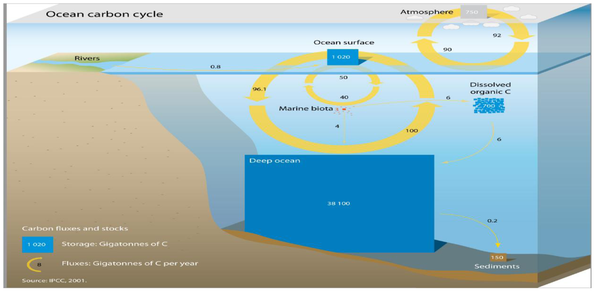
If a sustainable state is reached, fossil and renewable energy carriers can be treated the same way, because fossil carbon would then not be removed from lithosphere (and burned) at a rate that is higher than the rate at which it is transferred back into long-term storage of the lithosphere, via photosynthesis and biomass, which is deposited in sediments. This rate (excluding impermanent forest sequestration of CO₂) can be calculated as follows: The main deposition of organic matter occurs by oceanic sedimentation. An area of 1 m² sea bed sequesters 0.002 kg of organic carbon during a year [3,29]. According to the Intergovernmental Panel on Climate Change (IPCC) data in Figure 1, no more than 0.2 Gt C/a of carbon is absorbed globally by the sea sediments [30]. Since it can be assumed that CO₂ emissions are distributed all over the globe, an average CO₂ absorption yield of 3.925×10⁻⁴kg.C/a.m² can be derived for the Earth's surface area A_EARTH = 5.095×10¹⁴m², which does not restrict this area for other uses. Thus, the consumption of fossil energy demands a specific carbon sequestration area A_co2 of A_CO2 = 2,547.5m².a/kg.C. The area of A_co2 equals the modified carbon footprint of emitting 1 kg carbon of fossil origin per year into the biosphere. According to the concept of strong sustainability, applied here, the total modified fossil carbon footprint area $A_{C{O}_2}^{\mathit{\text{sum}}}$(the sum of all carbon areas in units of square meter) is not to exceed the biocapacity of Earth's surface of $A_{\mathit{\text{EARTH}}}:A_{C{O}_2}^{\mathit{\text{sum}}}<A_{\mathit{\text{EARTH}}}$. Otherwise, the carbon concentration within the biosphere will grow and finally exceed every planetary boundary [5]. The sum of the stocks of fossil carbon in the lithosphere and of the carbon stocks in the biosphere is constant. Thus, no more than 0.2 Gt C/a fossil carbon can be taken from lithosphere and burned worldwide if the carbon stocks of the atmosphere and the hydrosphere are not to grow, as is required for sustainability [3-5]. Instead currently 7 Gt C/a of carbon is burned [31] and the surface of 35 planet Earths would be necessary in order to absorb it.

On the other hand, the planet's soils are another sink for permanent storage of carbon, which have not yet been used. Carbon can be stored sustainably both in the soil and sea sediments (and not in the standing biomass of a not-growing forest area, as is assumed in calculations of the EF). Potentially, the soils are able to absorb 0.9 +/− 0.3 Gt C/a by changing land-use in a suitable manner [32], e.g., through restoration of forests, which decompose a large share of their organic matter into the soil [33]. This has the further advantage of restoring degraded soils as well as purifying surface and ground waters [32]. Furthermore, by increasing forest area and its biomass additional carbon can be taken out of the atmosphere. Using this potential, the specific carbon sequestration area A_CO2 could be reduced to 462.96m².a/kg.C [32].

3.2. Local Sustainable Yield

In order to achieve sustainability, the load on nature must in every instance remain below its maximum permissible borders. So, in addition to identifying and quantifying planetary boundaries, as is done by Rockström et al. [5], defining and determining the maximum permissible loads on nature everywhere objectively becomes one of the highest priorities and responsibilities of natural science. In case of imperfect scientific knowledge of the limits of the load, the precautionary principle must be applied and the exploitation must remain below the lowest possible value of the load.

Nevertheless, is it possible to define and determine a “maximum permissible border” in a way that will be widely accepted by all groups in society even though the groups have very different goals and objectives? In this regard, it is a matter of survival of “natural science” as an objective science, to liberate itself from the influence of interest groups. An impartial derivation of the physical limits of natural exploitation is a precondition for meeting these physical limits in practice, to ensure that they are widely accepted by all groups in society, even though they have very different goals and objectives.

Nowhere, local sustainable yields are to be exceeded [22,34]. As an example, it is only thus that soil degradation, or biodiversity loss due to loss of habitat (in accordance with the species/area relationship [35]), can be avoided. This contradicts the world averaging of area yield, as is standard in calculations of the EF [10,12,36]. In the averaging process, essential spatial details are lost, e.g., the EF cannot tell where the burden on nature due to the resource throughput occurs within a country, nor even whether it occurs inside or outside that country [37]. However, this is essential for striving at the goals of a worldwide reduction and equitable distribution of resources, as they are proposed for instance by Daly, White and others [1,2,38].

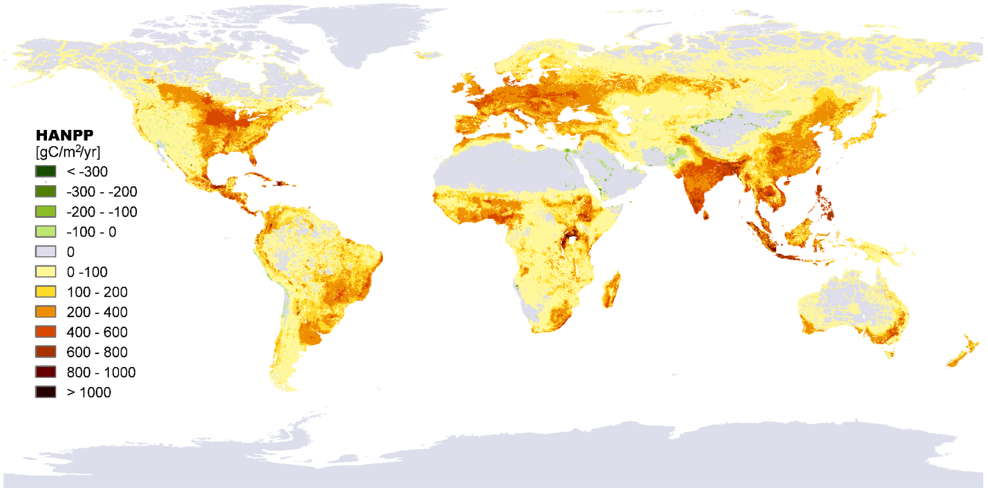
In contrast to the EF, the “Human Appropriation of Net Primary Production (HANPP)” calculates the difference between the “Net Primary Production” of biomass from potential natural vegetation (i.e., the vegetation that would prevail if human interference were absent) and the amount of biomass currently available in ecological cycles due to human intervention, within a defined land or water area [25,26]. With HANPP, the spatial disconnection between global biomass production and consumption can be mapped [39]. In Figure 2, the global distribution of local HANPP of soil areas is shown [40]. However, the HANPP does have shortcomings, as it is also founded on a non-sustainable yield of intensive area utilization, does not subtract the energy input, and excludes future yield decline due to over-exploitation.

In contrast to the EF and the HANPP, the “Sustainable Process Index (SPI)” and the “Dissipation Area Index (DAI)” consider the local sustainable yield of areas and take into account that these areas can deliver materials and energy permanently only with limited yield, and absorb waste and pollution to a restricted extent.

The SPI and DAI calculate the soil- and water areas needed to provide the raw materials and energy demands, as well as for the dissipation of pollution and waste, in a sustainable way [3,41], making use of the above four criteria of sustainability [3,4]. Thereby the DAI assesses the waste quality and quantity of different material and energy flows by discussing how fine substances have to be distributed so that they do not exceed the local assimilation capacity [42]. For example, in the case of nuclear energy, the sustainable absorption area of 1 kg radioactive waste (removing any contamination of biosphere) would be extraordinarily large. Hence, as a difference to the EF, the SPI and DAI are indicators of sustainability.

It is suggested here to combine the advantages of the EF with those of HANPP, SPI and DAI, using a sustainable local specific biomass yield y₀ (ϑ,φ) of soil and water area [22,34,43], in agreement with the sustainability criteria (of Section 1) [3,4] and with the precautionary principle [44]. y₀ (ϑ, φ) is the maximal sustainable amount of biomass per area (unit: kg C/(a.m²)) that can be harvested in a year at site (ϑ, φ) without causing irreversible yield reductions in the following years, for instance due to degradation of land or biodiversity. y₀ (ϑ,φ) equals the sustainable fraction of the HANPP, which is illustrated worldwide in Figure 2 [40], e.g., within a conservation area, y₀ (ϑ, φ) is either very small or zero, that way preserving biodiversity [35] and taking care of the most transgressed planetary boundary [5]. ϑ and ϕ symbolize the geographical width and length on the globe with its (average) radius R (R = 6.3674675 × 10⁶ m). Deriving y₀ (ϑ, φ) is a difficult task for biological science, but it is absolutely necessary if sustainability is to be attained [3,4,22,37,43] and humanity kept within safe operating space [5]. The four sustainability criteria [3,4] indicate, that the physical limits of nature's exploitation are local ones, with exceptions of those of the carbon emissions. If the local limits are surmounted, the carrying capacity of global nature for human life is reduced irreversibly and also the planetary limits are transgressed. On the other hand the local limits only can be considered if they are known. In case of insecurity, the exploitation must remain below the lowest possible value of the limit [44]. No research topic within environmental science appears to be more important than ascertaining the sustainable local biomass yield y₀ (ϑ,φ) (and not only the HANPP of Figure 2) all over the globe as soon as possible.

Analogous to the HANPP [25,26,40], it can be assumed that the human disturbance of nature due to the extraction of materials and energy, the emission of waste and pollution, or the building of human infrastructure, reduces the specific yield from its initial value y₀ (ϑ,φ) to a remaining yield of y₁ (ϑ,φ) within a land or water area, defined by the borders of φ₁ (ϑ) and (φ)₂(ϑ). The difference y₀ (ϑ,φ) − y₁ (ϑ,φ) equals the amount of biomass consumed by humans and their activities. y₁ (ϑ,φ) represents the share of sustainable local specific yield which is not affected by the disturbance and which remains available for further consumption. Integrating the reduction of specific yield y₀ (ϑ,φ) − y₁ (ϑ,φ) due to the human disturbance over the defined land or water area, its total resource yield is reduced by an amount Y of biomass [unit: kg.C/a]. In other words, a biomass amount Y is harvested from this area every year due to exploiting resources, emitting waste, or building:

$$Y=R^2.{\int }_{{\mathit{\vartheta }}_1}^{{\mathit{\vartheta }}_2}sin\mathit{\vartheta }d\mathit{\vartheta }{\int }_{{\phi }_1(\mathit{\vartheta })}^{{\phi }_2(\mathit{\vartheta })}d\phi [y_0(\mathit{\vartheta },\phi )-y_1(\mathit{\vartheta },\phi )]$$

(1)

Y does not contain any input of fossil energy or of other non-renewable resources, e.g., in the case of fishing, the fish biomass yield comes not only from the water area, but from its sum with the carbon sequestration area of the fuel used by the fishing vessel and with the area necessary for producing the abiotic resources which are demanded throughout the lifecycle (from cradle to grave) of the ship (divided through the ship lifetime) [37]. Using all the available biomass without leaving any remainder, the maximal possible sustainable specific yield ȳ of the defined land or water area results from:

$$\stackrel{\overline{y}={\int }_{{\mathit{\vartheta }}_1}^{{\mathit{\vartheta }}_2}sin\mathit{\vartheta }d\mathit{\vartheta }{\int }_{{\phi }_1(\mathit{\vartheta })}^{{\phi }_2(\mathit{\vartheta })}d\phi [y_0(\mathit{\vartheta },\phi )]}{}/\underset{{\int }_{{\mathit{\vartheta }}_1}^{{\mathit{\vartheta }}_2}sin\mathit{\vartheta }d\mathit{\vartheta }[{\phi }_2(\mathit{\vartheta })-{\phi }_1(\mathit{\vartheta })]}{}$$

(2)

If Y is caused by human intervention in a natural system, such as the exploitation of 1 kg of a resource or the emission of 1 kg waste per year, this claims an area of A_MEF square meter, which is then (as a difference to the specific carbon sequestration area A_CO2 of Section 3.2) not available any more for any other kind of interference:

$$A_{\mathit{\text{MEF}}}=\stackrel{y}{}/\underset{\overline{y}}{}$$

(3)

The specific area A_MEF (unit: m².a/kg.C) refers to the contribution to a modified EF, corresponding to the areas of the SPI [3] and the DAI [42], which together indicate the area demand of a particular intervention in a natural system. The specific area demand A_MEF and the sum of all demands $A_{\mathit{\text{MEF}}}^{\mathit{\text{sum}}}$can be compared with the supply of the existing area, thus representing the actual biocapacity. The total biocapacity of the globe equals its surface area: A_EARTH=4.π.R².

3.3. Considering Intertemporal Effects

An intervention in a natural system in a specific year might cause yield reductions from y₀ (ϑ,ϕ) to $y_0^n$(ϑ,(ϕ))in the subsequent n years (0 < n ≤ N₁).All these reductions must be considered. The EF, however, ignores these future effects [19,23,45], just as the Equations (1–3) do. Summing up all those future yield reductions, as a difference to the amount Y of Equation (1) a larger amount Y₁^int of biomass is harvested by an intervention into the natural system in the first year, claiming a larger specific area $A_{\mathit{\text{MEF}}}^{int}$

$$A_{\mathit{\text{MEF}}int}=\stackrel{Y_1^{int}}{}/\underset{\overline{y}}{}$$

(4)

$$Y_1^{int}=R^2\cdot {\sum }_{n=1}^{N_1}{\int }_{{\mathit{\vartheta }}_1}^{{\mathit{\vartheta }}_2}sin\mathit{\vartheta }d\mathit{\vartheta }{\int }_{{\phi }_1(\mathit{\vartheta })}^{{\phi }_2(\mathit{\vartheta })}d\phi [y_{\text{o}}^n(\mathit{\vartheta },\phi )-y_1^n(\mathit{\vartheta },\phi )]$$

(5)

With the aid of “Land and Ecosystem Accounts (LEAC)” [28], it is possible to find such variations $y_o^n$ (ϑ,φ)of the sustainable local yield with the years n in a dynamic approach [45], e.g., in the EF a built-up land is treated in the same way, as a crop land [10-12]. Nevertheless there is a large difference between them [45]. For the latter, the future yield does not necessarily drop due to agriculture, producing the crops: $y_0^n(\mathit{\vartheta },\phi )=y_0(\mathit{\vartheta },\phi )$for n > 0. However, in cases where the soil is sealed in order to build human infrastructure, the future yield is reduced to zero for a long time, or forever:

$$y_0^n(\mathit{\vartheta },\varphi ){|}_{0<n<N_1}=0,\text{with}{N}_1\gg 1or{N}_1=\infty$$

(6)

$y_1^{int}$ Y₁^int and the built-up area A_MEFint become very large in this case, taking into account the fact that irreversible reductions of biocapacity resulting from land take are incompatible with sustainability. Due to the incorrect treatment of built-up land within the EF, this appears not to have increased since industrialization [15].

Equation (5) accounts for all future yield reductions of soil or water area due to overuse in the first year, e.g., due to land or biodiversity degradation. Overuse causes a reduction of the yields $y_{m-1}^n$(ϑ, (ϕ))and biomass amounts $Y_m^{int}$, which can be harvested in the following years m>1, since their consumption has already been realized in the first year m = 1:

$$Y_m^{int}=R^2{\sum }_{n=1}^{N_1}{\int }_{{\mathit{\vartheta }}_1}^{{\mathit{\vartheta }}_2}sin\mathit{\vartheta }d\mathit{\vartheta }{\int }_{{\phi }_1(\mathit{\vartheta })}^{{\varphi }_2(\mathit{\vartheta })}d\varphi [y_{m-1}^n(\mathit{\vartheta },\phi )-y_m^n(\mathit{\vartheta },\varphi )]$$

(7)

3.4. Considering Abiotic Resources

Abiotic resources are taken into consideration by the Equations (1) to (7), just as it is done by the SPI, the DAI and by the “Environmentally Weighted Material Consumption (EMC)” [27]. The SPI and the DAI find out how much of the existing limited area between the ecosphere and the anthroposphere is used up by a unit flux of material of all sorts in one direction [3], or waste of every kind in the opposite direction [42]. This corresponds to Equation (1): There, the specific biomass yield of the soil and water areas is reduced from y₀(ϑ,φ) to y₁ (ϑ,φ) due to these fluxes. A_MEF of Equation (3) indicates how much soil or water area is necessary for them. Furthermore, the EMC takes all material fluxes throughout a product's life cycle into account and weights them according to their objectively quantified environmental impacts [27]. The impacts are expressed in different units: For instance, land use (in unit of m²), impact on climate change (in CO₂-equivalents), toxicity (in kg 1,4-dichlorbenzene equivalents), waste production (in kg over product life cycle), depletion (in kg antimony equivalents), the loss of biodiversity (in m²), taking care the loss of habitat [27]. By deriving the contributions of these entirely different impacts to the reduction of the specific area yields y₀ (ϑ,φ) according to Equation (1), they can be converted into one common unit. In this way the area A_MEF of Equation (3) (or A_MEFint of Equation (4) in the case of intertemporal effects) can be found, which is used up by the flux of 1 kg of material, waste or pollutant of any kind in a sustainable state. This way, the results of the EMC can be used for calculating the contributions to a modified ecological footprint A_MEF (or A_MEFint) with one exception.

3.5. Considering Resource Depletion

The depletion impact of EMC and the increasing scarcity of non-renewable resources due to their consumption cannot be considered in this way, however. Neither the Equations (1–7), nor the SPI, the DAI, nor the EF allow for it. Depletion can be related to the exergy loss due to the utilization of non-renewable resources. If a society consumes exergy resources at a faster rate than they are renewed by solar radiation, it will not be sustainable [46]. In light of this, the present industrial society is obviously unsustainable and is facing collapse [47,48]. Thus it follows that this consumption of natural exergy supply is also to be taken into consideration in the calculations of an EF.

Depletion is only zero if non-renewable resources are completely recycled at a rate r of r = 100%. For rates below this (r < 100%) the fraction (100 − r)% of the resources is distributed in the environment usually with concentrations smaller than the original ones. For example the production of one metric ton of austenitic stainless steel requires 79 GJ from virgin materials and only 26 GJ in the case of 100% recycling [49]. Therefore at least the energy of 53 GJ per ton (79 − 26 = 53) is lost, if the steel is not recycled after its use and thrown away. In this way additional energy is required, in order to remove the resources from the environment and to compensate for this exergy loss by raising concentrations to the original value again. Depletion can be taken into account by converting solar energy into the surface area A_DEP necessary to produce this energy, as it is done by Nguyen [50] and by including this area into the modified EF. It follows from this that, in the case of fossil energy carriers, not only the carbon absorption areas A_CO2 but also the areas necessary for harvesting the equivalent amount of solar energy need to be included in a modified EF [51]. The EF, however, considers only the one or the other.

The concept of strong sustainability requires that stocks of natural capital be maintained, so that they are available for use by future generations [52]. Using non-renewable resources, material is conserved due to the laws of physics. Nevertheless, entropy might grow considerably during the transformation of the materials extracted from nature into waste and pollutants. If non-renewable resources, for example, are ultimately distributed in a dilute form in soil or sea sediments, the amount of solar exergy required is extremely high, in order to raise their concentrations sufficiently for reuse. However, Nguyen compensates only incompletely for this large exergy loss through solar energy [50]. Still, in contradiction to strong sustainability, non-renewable resources would be used excessively, to the disadvantage of future generations [53].

4. Conclusions

The EF converts the consumption of biotic resources in a very straightforward way into the share of biologically productive area existing on planet Earth. Therefore, it is very successful in raising public awareness. However, this simplicity is achieved at the cost of producing an incomplete picture, which results in three major weaknesses.

First, the EF is not an indicator of sustainability or of intergenerational justice, because it allows excessively large non-sustainable biomass area yields, and ignores their future reduction due to overexploitation. Furthermore, it underestimates the absorption areas for CO₂, excludes the area demand for throughput of abiotic resources, and does not consider depletion.

Secondly, the EF is not an indicator of intragenerational justice, because it undervalues the environmental burden of non-renewable resources relative to those of renewable ones, and operates with non-local average yields.

Thirdly, with the EF's global yield averaging, spatial information is lost regarding where resources are taken from nature and where waste and pollutants are returned to it. Therefore, the environmental burden of resource throughput of a product, a service, a human being, or a nation cannot be compared with that of another product, service, human being, or nation. For this reason, the EF is not suitable for informing about all the costs of a purchase decision, and only incompletely successful in enabling sensible decisions between life-styles or economic policies.

The EF can be improved if the suggestions of critics and authors of competing indicators are adopted in order to modify it. The main idea of a modified EF is the derivation of the size of the soil and water area demanded by a unit resource or waste of every kind, which is taken from it, or given to it, in a sustainable way, just as in the cases of SPI and DAI. Its derivation is based on the local sustainable area yield, proposed also by Ferng [22,34]. It specifies which share of the biomass area yield can be harvested without reducing future area yield. By use of the HANPP, how much of this yield is used up by resource extraction, waste absorption or build-up of human infrastructure, can be calculated. As in the case of the EMC, SPI and DAI, also the area demand of abiotic materials can be derived. In addition to this, the area demand for harvesting solar exergy is considered, which is necessary to compensate for exergy loss of non-renewable resource use.

In a sustainable state, the sum of areas $(A_{\mathit{\text{MEF}}int}^{\mathit{\text{sum}}}+A_{\mathit{\text{DEP}}}^{\mathit{\text{sum}}})$calculated in this way (the areas A_MEFint for extracting materials with low entropy from nature, for their return to it with high entropy, for built structures and A_DEP for compensating the exergy loss) are not to exceed the Earth's surface: $A_{\mathit{\text{MEF}}int}^{\mathit{\text{sum}}}+A_{\mathit{\text{DEP}}}^{\mathit{\text{sum}}}<A_{\mathit{\text{EARTH}}}$Besides this, the CO₂ emissions are limited to the absorption of CO₂ by sustainable sinks: $A_{C{O}_2}^{\mathit{\text{sum}}}<A_{\mathit{\text{EARTH}}}$. As an approximation, the two limits can be combined: $A_{\mathit{\text{MEF}}int}^{\mathit{\text{sum}}}+A_{C{O}_2}^{\mathit{\text{sum}}}+A_{\mathit{\text{DEP}}}^{\mathit{\text{sum}}}<2.A_{\mathit{\text{EARTH}}}$.

In addition to the demand of an area by unit of resource throughput, the demand of resource throughput by unit of consumption must be found out. Usually, “Life Cycle Assessment” [54,55] or “Material Input Per unit of Service (MIPS)” [56,57] is applied for the calculation of the resource demand for the lifecycle of a product and for the environmental impact of its consumption as well, and “Input Output Analysis” is applied for resource demand of consumption within nations, regions, economic sectors, or of socioeconomic groups [7,55,58]. These studies can be simplified, by ecolabeling a resource with its demand of Earth's area on the spot where it is extracted from nature. The area demand of a commodity can then be composed of those of the labeled resources needed for its production in a simple manner [2]. Thus the commodities can also be ecolabeled with their area demand, in addition to labeling them with a price. This is a precondition for integrating natural limits via the prices (containing all positive and negative costs, externalized so far) into economic selfcontrolling mechanisms reducing this way the demand of resource areas $(A_{\mathit{\text{MEF}}int}^{\mathit{\text{sum}}}+A_{C{O}_2}^{\mathit{\text{sum}}}+A_{\mathit{\text{DEP}}}^{\mathit{\text{sum}}})$to their supply (2.A_EARTH). Thereby not necessarily the usual “homo economicus” has to be assumed, who makes exclusively rational decisions during purchasing a product. Because the sales of products not only rise (drop), since their prices drop (rise) but also because their purchase is ecologically and socially fair (unfair), due to the perfect internalization of all external costs…” In summary, an indicator of just resource distribution between and within generations, and a benchmark for decision-making between alternative types of consumption, life-styles and economic policies, results.

References

- Daly, E.D. Allocation, distribution, and scale: Towards an economics that is efficient, just and sustainable. Ecol. Econ. 1992, 6, 185–193. [Google Scholar]
- Aubauer, H.P. A just and efficient reduction of resource throughput to optimum. Ecol. Econ. 2006, 58, 637–649. [Google Scholar]
- Krotscheck, C.; Narodoslawsky, M. The Sustainable Process Index: A new dimension in ecological evaluation. Ecol. Eng. 1996, 6, 241–258. [Google Scholar]
- Moser, A. Task Group Ecological Bioprocessing of the European Federation of Biotechnology: End Report; Österreichische Gesellschaft für Bioprozeβtechnik (ÖGBPT): Graz, Austria, 1993. [Google Scholar]
- Rockström, J.; Steffen, W.; Noone, K.; Persson, Å.; Chapin, F.S.I.; Lambin, E.; Lenton, T.M.; Scheffer, M.; Folke, C.; Schellnhuber, H.J.; Nykvist, B.; de Wit, C.A.; Hughes, T.; van der Leeuw, S.; Rodhe, H.; Sörlin, S.; Snyder, P. K.; Costanza, R.; Svedin, U.; Falkenmark, M.; Karlberg, L.; Corell, R.W.; Fabry, V.J.; Hansen, J.; Walker, B.; Liverman, D.; Richardson, K.; Crutzen, P.; Foley, V.J. A safe operating space for humanity. Nature 2009, 461, 472–475. [Google Scholar]
- Pillarisetti, J.R.; van den Bergh, J.C.J.M. Sustainable nations: What do aggregate indexes tell us? Environ. Dev. Sustain. 2010, 12, 49–62. [Google Scholar]
- Wiedmann, T.; Minx, J.; Barrett, J.; Wackernagel, M. Allocating ecological footprints to final consumption categories with input-output analysis. Ecol. Econ. 2006, 56, 28–48. [Google Scholar]
- WWF Zoological Society of London, Global Footprint Network and Twente Water Centre. Living Planet Report 2008; World-Wide Fund for Nature International (WWF): Gland, Switzerland, 2008. [Google Scholar]
- Kitzes, J.; Galli, A.; Bagliani, M.; Barrett, J.; Dige, G.; Ede, S.; Erb, K.; Giljum, S.; Haberl, H.; Hails, C.; Jolia-Ferrier, L.; Jungwirth, S.; Lenzen, M.; Lewis, K.; Loh, J.; Marchettini, N.; Messinger, H.; Milne, K.; Moles, R.; Monfreda, C.; Moran, D.; Nakano, K.; Pyhälä, A.; Rees, W.; Simmons, C.; Wackernagel, M.; Wada, Y.; Walsh, C.; Wiedmann, T. A research agenda for improving national Ecological Footprint accounts. Ecol. Econ. 2009, 68, 1991–2007. [Google Scholar]
- Monfreda, C.; Wackernagel, M.; Deumling, D. Establishing national natural capital accounts based on detailed Ecological Footprint and biological capacity assessments. Land Use Policy 2004, 21, 231–246. [Google Scholar]
- Wackernagel, M.; Monfreda, C.; Schulz, N.B.; Erb, K.; Erb, K.-H.; Haberl, H.; Krausmann, F. Calculating national and global ecological footprint time series: Resolving conceptual challenges. Land Use Policy 2004, 21, 271–278. [Google Scholar]
- Kitzes, J.; Wackernagel, M. Answers to common questions in Ecological Footprint accounting. Ecol. Indicat. 2009, 9, 812–817. [Google Scholar]
- Wackernagel, M. Methodological advancements in footprint analysis. Ecol. Econ. 2009, 6, 1925–1927. [Google Scholar]
- Lal, R. Carbon Sequestration. Phil. Trans. Biol. Sci. 2008, 363, 815–830. [Google Scholar]
- Haberl, H.; Erb, K.-H.; Krausmann, F. How to calculate and interpret ecological footprints for long periods of time: The case of Austria 1926–1995. Ecol. Econ. 2001, 38, 25–45. [Google Scholar]
- Stöglehner, G. Ecological footprint—a tool for assessing sustainable energy supplies. J. Clean. Prod. 2003, 11, 267–277. [Google Scholar]
- Hall, D.O. Photobiological energy conversion. FEBS Lett. 1976, 64, 6–16. [Google Scholar]
- Schwarzlmüller, E. Human appropriation of aboveground net primary production in Spain, 1955–2003: An empirical analysis of the industrialization of land use. Ecol. Econ. 2009, 69, 282–291. [Google Scholar]
- Lenzen, M.; Hansson, C.B.; Bond, S. On the bioproductivity and land-disturbancemetrics of the Ecological Footprint. Ecol. Econ. 2007, 61, 6. [Google Scholar]
- Fiala, N. Measuring sustainability: Why the ecological footprint is bad economics and bad environmental science. Ecol. Econ. 2008, 67, 519–525. [Google Scholar]
- Kitzes, J.; Moran, D.; Galli, A.; Wada, Y.; Wackernagel, M. Interpretation and application of the Ecological Footprint: A reply to Fiala. Ecol. Econ. 2009, 68, 929–930. [Google Scholar]
- Ferng, J.-J. Local sustainable yield and embodied resources in ecological footprint analysis—a case study on the required paddy field in Taiwan. Ecol. Econ. 2005, 53, 415–430. [Google Scholar]
- Lenzen, M.; Shauna A Murray, S.A. The Ecological Footprint—Issues and Trends; ISA Research Paper 01-03; The University of Sydney: Sydney, Australia, 2003. [Google Scholar]
- Best, A.; Gilium, S.; Simmons, C.; Blobel, D.; Lewis, K.; Hammer, M.; Cavalieri, S.; Lutter, S.; Maguire, C. Potential of the Ecological Footprint for Monitoring Environmental Impacts from Natural Resource Use: Analysis of the Potential of the Ecological Footprint and Related Assessment Tools for Use in the EU's Thematic Strategy on the Sustainable Use of Natural Resources; Report to the European Commission DG Environment; SERI: Vienna, Austria, 2008; pp. 1–304. [Google Scholar]
- Haberl, H.; Wackernagel, M.; Krausmann, F.; Erb, K.-H.; Monfreda, C. Ecological footprints and human appropriation of net primary production: A comparison. Land Use Policy. 2004, 21, 279–288. [Google Scholar]
- Erb, K.-H.; Krausmann, F.; Gaube, V.; Gingrich, S.; Bondeau, A.; Fischer-Kowalski, M.; Haberl, H. Analyzing the global human appropriation of net primary production—processes, trajectories, implications. An introduction. Econ. Econ. 2009, 69, 250–259. [Google Scholar]
- van der Voet, E.; Oers, L.V.; Nikolic, I. Dematerialisation: Not Just A Matter of Weight; Centre of Environmental Science (CML), Section and Substances & Products, Leiden University: Leiden, The Netherlands, 2003; pp. 1–177. [Google Scholar]
- Weber, J.-L. Implementation of land and ecosystem accounts at the European Environment Agency. Ecol. Econ. 2007, 61, 695–707. [Google Scholar]
- Krotscheck, C.; König, F.; Obernberger, I. Ecological assessment of integrated bioenergy systems using the Sustainable Process Index. Biomass Bioenerg. 2000, 18, 341–368. [Google Scholar]
- Intergovernmental Panel on Climate Change (IPCC). Climate Change 2001: The Scientific Basis; Cambridge University Press: Cambridge, UK, 2001. [Google Scholar]
- Pacala, S.; Socolow, R. Stabilization wedges: solving the climate problem for the next 50 years with current technologies. Science 2004, 305, 968–972. [Google Scholar]
- Lal, R. Soil carbon sequestration to mitigate climate change. Geoderma 2004, 123, 1–22. [Google Scholar]
- Luyssaert, S.; Schulze, E.-D.; Börner, A.; Knohl, A.; Hessenmöller, D.; Law, B.E.; Ciais, P.; Grace, J. Old-growth forests as global carbon sinks. Nature 2008, 455, 213–215. [Google Scholar]
- Aubauer, H.P. Biologisch produktive Bodenflächen als Voraussetzung zukünftigen Lebens. Wissenschaft&Umwelt Interdisziplinär Boden-Markierungen 2004, 8, 11–24. [Google Scholar]
- Desmet, P.; Cowling, R. Using the species-area relationship to set baseline targets for conservation. Ecol. Soc. 2004, 9, 1–15. [Google Scholar]
- Wackernagel, M.; Rees, W.E. Our Ecological Footprint: Reducing Human Impact on the Earth; New Society Publishers: Gabriola Island, Canada, 1996. [Google Scholar]
- Lenzen, M.; Murray, S.A. A modified ecological footprint method and its application to Australia. Ecol. Econ. 2001, 37, 229–255. [Google Scholar]
- White, T.J. Sharing resources: The global distribution of the Ecological Footprint. Ecol. Econ. 2007, 64, 402–410. [Google Scholar]
- Erb, K.-H.; Krausmann, F.; Lucht, W.; Haberl, H. Embodied HANPP: Mapping the spatial disconnect between global biomass production and consumption. Ecol. Econ. 2009, 69, 328–334. [Google Scholar]
- Haberl, H.; Erb, K.-H.; Krausmann, F.; Gaube, G.; Bondeau, A.; Plutzar, C.; Gingrich, S.; Lucht, W.; Fischer-Kowalski, M. Maps on the global human appropriation of net primary production (HANPP) in the year 2000. Quantifying and mapping the global human appropriation of net primary production in Earth's terrestrial ecosystem. Proc. Natl. Acad. Sci. USA 2007, 104, 12942–12947. [Google Scholar]
- Stöglehner, G.; Narodoslawsky, M. Implementing ecological footprinting in decision-making processes. Proc. Natl. Acad. Sci. 2008, 25, 421–431. [Google Scholar]
- Eder, P.; Narodoslawsky, M. What environmental pressures are a region's industries responsible for? A method of analysis with descriptive indices and input-output models. Ecol. Econ. 1999, 29, 359–374. [Google Scholar]
- Ferng, J.-J. Resource-to-land conversions in ecological footprint analysis: The significance of appropriate yield data. Ecol. Econ. 2007, 62, 379–382. [Google Scholar]
- Principle 15 of the “Rio Declaration on Environment and Development” of “The United Nations Conference on Environment and Development” Rio de Janeiro from 3 to 14 June 1992; United Nations: New York, NY, USA, 1992. Available online: http://en.wikipedia.org/wiki/Rio_Declaration_on_Environment_and_Development (accessed on 12 August 1992).
- Lenzen, M.; Wiedmann, T.; Foran, B.; Dey, Ch.; Widmer-Cooper, A.; Williams, M.; Ohlemüller, R. Forecasting the Ecological Footprint of Nations: A Blueprint for a Dynamic Approach; ISA Research Paper 07/01. Sydney University: Sydney, Australia, June 2007. Available online: http://www.isa.org.usyd.edu.au/publications/DEF.pdf (accessed on 1 February 2011).
- Szargut, J.T. Anthropogenic and natural exergy losses (exergy balance of the Earth's surface and atmosphere. Energy. 2003, 28, 1047–1054. [Google Scholar]
- Wall, G.; Gong, W. On exergy and sustainable development—Part 1: Conditions and concepts. Exergy Int. J. 2001, 1, 128–145. [Google Scholar]
- Gong, M.; Wall, G. On exergy and sustainable development—Part 2: Indicators and methods. Exergy Int. J. 2001, 1, 217–233. [Google Scholar]
- Johnson, J.; Reck, B.K.; Wang, T.; Graedel, T.E. The energy benefit of stainless steel recycling. Energ. Policy 2008, 36, 181–192. [Google Scholar]
- Nguyen, H.X.; Yamamoto, R. Modification of ecological footprint evaluation method to include non-renewable resource consumption using thermodynamic approach. Resour. Conserv. Recycl. 2007, 51, 870–884. [Google Scholar]
- Szargut, J.; Stanek, W. Thermo-climatic cost of the domestic consumption products. Energy 2010, 35, 1196–1199. [Google Scholar]
- Neumayer, E. Weak Versus Strong Sustainability, 2nd ed.; Edward Elgar Publishing: Cheltenham, UK, 2003. [Google Scholar]
- Heijungs, R.; Guinée, J.; Huppes, G. Impact Categories for Natural Resources and Land Use; CML Report 138; Section Substances & Products, Centre of Environmental Science (CML); Leiden University: Leiden, The Netherlands, 1997. [Google Scholar]
- Huijbregts, M.A.J.; Hellweg, S.; Frischknecht, R.; Hungerbühler, K.; Hendriks, A.J. Ecological footprint accounting in the life cycle assessment of products. Ecol. Econ. 2008, 64, 798–807. [Google Scholar]
- Hinterberger, F.; Luks, F.; Schmidt-Bleek, F. Material flows vs. “natural capital”: What makes an economy sustainable? Ecol. Econ. 1997, 23, 1–14. [Google Scholar]
- Schmidt-Bleek, F. Wieviel Umwelt braucht der Mensch? MIPS, das Maβ für ökologisches Wirtschaften [How much environment do we need? MIPS, the measure for ecologically sound economic performance; Birkhäuser: Berlin, Germany, 1994. [Google Scholar]
- Turner, K.; Lenzen, M.; Wiedmann, T.; Barrett, J. Examining the global environmental impact of regional consumption activities—Part 1: A technical note on combining input-output and ecological footprint analysis. Ecol. Econ. 2007, 62, 37–44. [Google Scholar]
- Penela, A.C.; Villasante, C.S. Applying physical input-output tables of energy to estimate the energy ecological footprint (EEF) of Galicia (NW Spain). Energ. Policy 2008, 36, 1148–1163. [Google Scholar]
© 2011 by the authors; licensee MDPI, Basel, Switzerland. This article is an open access article distributed under the terms and conditions of the Creative Commons Attribution license (http://creativecommons.org/licenses/by/3.0/).
Share and Cite
Aubauer, H.P. Development of Ecological Footprint to an Essential Economic and Political Tool. Sustainability 2011, 3, 649-665. https://0-doi-org.brum.beds.ac.uk/10.3390/su3040649
Aubauer HP. Development of Ecological Footprint to an Essential Economic and Political Tool. Sustainability. 2011; 3(4):649-665. https://0-doi-org.brum.beds.ac.uk/10.3390/su3040649
Chicago/Turabian StyleAubauer, Hans P. 2011. "Development of Ecological Footprint to an Essential Economic and Political Tool" Sustainability 3, no. 4: 649-665. https://0-doi-org.brum.beds.ac.uk/10.3390/su3040649