1. Introduction
Warming of the global climate system is unequivocal [
1]. Even though there is a scientific consensus on the existence of climate change and the human role in it [
2], the role of cities and urban activities in the global warming has been hotly debated in recent years [
3,
4]. The general opinion is that sprawling urban development is detrimental to the environment and that the denser the structures are the better. When urban structures grow outwards, the people living in loosely populated surrounding areas are more car-dependent and tend to live in less eco-efficient apartments. Consequently, in the literature the studies on the effects of sprawl have mostly investigated emissions from driving and home heating [
5,
6,
7].
However, urbanization and its supporting infrastructure
per se do not alone cause climate change: it is also the people–living, moving, and consuming in cities. Thus, it is not only the emissions from heating, electricity and driving that need to be taken into account but also the emissions from all other consumption must be kept in mind. Only with this kind of holistic assessment, a sufficient level of understanding about the greenhouse gas consequences of sprawl can be reached. Similar consumption-based assessments are gaining more and more foothold in the literature, and it is acknowledged that they suit particularly well for urban environments and should at least act as complements to the traditional production-based methods [
8,
9].
The proliferation of semi-detached and detached houses at the urban edge is one of the best-known characteristics of sprawl [
10,
11]. Combined with looser suburban structures and less accessible public transportation, sometimes not even very far from the urban core, this less dense low-rise living represents the sprawl in an intra-urban context. Thus, in this paper, we distinguish between different types of houses and analyze the differences in typically inner-city high-rise and typical suburban low-rise lifestyles and their GHG effects. Furthermore, it has been argued that one reason for low-rise living are policies that encourage home owning and implicitly encourage people to move away from higher density living [
11]. The analysis was done within a single metropolis, the Helsinki Metropolitan Area [HMA], in Finland. The HMA is the capital region of Finland that consists of four cities with more than one million inhabitants. This type of sprawl is a very interesting phenomenon to analyze as within a single metropolis the residents still maintain rather close proximity to all the consumption opportunities that the city or metropolitan area offers but rely predominantly on private driving and have more living space to be heated, furnished, and filled with domestic appliances.
In this study, we assess households' GHG impacts by calculating their consumption-based carbon footprints,
i.e., direct and indirect life-cycle greenhouse gas emissions either home or elsewhere, which are ultimately caused by consumption of products and services [
39]. Following the literature, the footprints are calculated by combining the input data from a Finnish household budget survey with the environmentally-extended input-output [EE I-O] model ENVIMAT based on the Finnish economy [
13,
14]. The carbon footprints are further elucidated with a multivariate regression analysis. What we add to the previous discussions on sprawl is the perspective of how emissions from consumption in its broad sense, beyond those from solely driving and housing energy, affect the GHG consequences and their policy implications within a single metropolitan area. The study sheds light on the effects of proximity on consumption, suggesting that, in denser agglomerations, indirect emissions from consumption of goods and services grow, as has been argued to happen on a country level [
12]. Consumption-based approach is expected to facilitate the understanding of urban lifestyles that are related to urban sprawl. We demonstrate that the GHG impacts of consumption vary by the type of dwelling, but the overall differences between low- and high-rise dwellers remain rather minor and much more equivocal than previously assumed. We believe that an understanding of both the differences and similarities in lifestyles offers important insights for sustainable policy-design and urban planning.
The structure of our paper is as follows: first, the research design,
i.e., consumption data, both the methods and research process, is presented in
Section 2. The results are presented in
Section 3, and a discussion follows in
Section 4. We finish with conclusions in
Section 5.
2. Research Design
2.1. The Case Area and Input Data
The selected case area, the HMA, with a population of over one million, is the capital region of Finland and consists of four cities: Helsinki, Vantaa, Espoo, and Kauniainen. It is known that the Helsinki region has spread out widely, and the spreading out still continues [
15]. The area shares many traits with the globe’s biggest metropolises, the results thus giving indication of more general patterns. Furthermore, within such a clearly defined and geographically restricted area, some of the most uncertain assumptions of input-output technique, such as that of homogenous prices, are closer to reality. In addition, the HMA is interconnected by an extensive public transportation network, and possibilities to choose between private and public modes of transport are quite diverse, with free parking made available for those who need private cars to reach public transport hubs. In line with the sprawl hypothesis, the division of housing types within the area is clear: the city core is dominated by apartment houses, and semi-detached and detached houses are the main types of houses at the edge. Some key characteristics of the four areas can be found from the
Table 1.
Table 1.
Key characteristics of Helsinki Metropolitan Area (HMA) areas [
36,
46].
Table 1.
Key characteristics of Helsinki Metropolitan Area (HMA) areas [36,46].
| | HELSINKI | ESPOO | VANTAA | KAUNIAINEN |
|---|
| Population size (31.12.2012) | 603,968 | 256,824 | 205,312 | 8,910 |
| Density (inhabitants per km2) | 2,826 | 823 | 861 | 1,513 |
| Apartment building of housing stock (%) | 86 | 58 | 62 | 46 |
The input data consists of the latest Finnish Household Budget Survey data from 2006 [
16]. The dataset is cross-sectional in nature, and alongside the actual detailed consumption expenditure data, arranged according to the international COICOP (Classification of Individual Consumption by Purpose) classification, the data contain a wide array of background and income information for each household. Budget Survey is a sample survey study that employs a one-stage stratified cluster sampling design. The final sample size of the survey was 4,007 households. However, the original sample was double the size, and the magnitude of response was only 47.7%—a situation that can be described as under coverage. However, non-response bias can be significantly reduced using weight coefficients, and systematic biases can be avoided. In order to allow generalization of our results, the weight coefficients are utilized throughout this paper.
In this paper, the sample of households is restricted to the HMA. Even if, with its approximately one million inhabitants, the Helsinki Metropolitan Area is relatively small in size when compared to the world’s largest megacities, it has many characteristics of a metropolis: a little more than a third of Finland’s GDP is produced there, both the levels of education and wages are higher than the average, and there is an extensive public transport network. According to Alanen
et al., the challenges of metropolises are often different than in the rest of Finland, but similar to the other metropolises [
17].
In order to support our choice to restrict the sample to the Helsinki Metropolitan Area, it can be briefly compared to the rest of the country. In short, the households in the metropolitan area are richer and smaller: the average household size in the HMA is 1.93, whereas it is 2.16 in the rest of country. Likewise, the average disposable income per household is €42,533 in the HMA, whereas it is €33,634 for the rest of country. Furthermore, for households living in the metropolitan area, the average amount of cars per household is more than a one-third lower than in the rest of the country and the share of carless households in the HMA is 20 percentage points higher, illustrating the availability of public transportation there. In our data, 59% of households living in Helsinki metropolitan area are homeowners. In the rest of the country the figure is 70%. Furthermore, in the metropolitan area, the share of households living in low-rise dwellings (i.e., in detached or semi-detached houses) is relatively low and is 38 percentage points lower than in the rest of the country.
Table 2 describes our sample data. The house types are divided to low-rise and high-rise categories. The low-rise category consists of households living in either detached (n = 97) or semi-detached houses (n = 73), and the high-rise one refers to households living in apartment houses (n = 398).
Table 2.
Descriptive statistics for high-rise and low-rise sub-samples.
Table 2.
Descriptive statistics for high-rise and low-rise sub-samples.
| | LOW-RISE (n = 170) | HIGH-RISE (n = 389) |
|---|
| Household characteristics: | | |
| Disposable income (€) | 62 719 | 35 410 |
| Consumption expenditure (€) | 46 141 | 29 710 |
| Average household size | 2.45 | 1.75 |
| Number of cars per household | 1.00 | 0.51 |
| Share of carless households | 0.26 | 0.53 |
| Share of households with children | 0.37 | 0.19 |
| Building type characteristics: | | |
| Average living area (square meters) | 118.31 | 61.28 |
| Per-capita living area (square meters) | 48.28 | 35.05 |
| Number of rooms per person* | 1.93 | 1.53 |
| Share of owner-occupied dwellings | 0.81 | 0.51 |
In household characteristics, there are some interesting differences between sub-samples. As expected, households living in semi-detached or detached houses are the wealthiest and own the most cars, since the hypothesis was that low-rise lifestyle is a lifestyle leading to car-dependency. Accordingly, more than half of the households in the apartment houses are carless, the precise figure being 53%, which indicates that the apartment houses in the Helsinki Metropolitan Area are, on average, located close to public transportation facilities. Furthermore, families with children are likely to live in the areas of sprawl, i.e., in detached or semi-detached houses, the share of families with children in apartment houses being less than one-fifth. Interestingly, 42% of these high-rise households with children are single-parent families.
In addition, housing type differences are rather expected. Average living space in low-rise houses is 118.3 m
2, almost twice the living area of apartment houses. When compared on per-capita level, the living area in low-rise houses is 1.4 times bigger than in high-rise ones. However, the actual difference is lower due to the fact that the apartment dwellers use shared spaces, such as hallways and storage facilities, which are not included in these self-reported figures. Nevertheless, they also create GHG emissions. These common spaces in apartment buildings are taken into account in this paper by allocating the emissions from them for their residents. This allocation is based on official statistics on the finance of housing companies [
18]. There are also significant differences in the share of owner-occupied dwellings between the sub-samples. As expected, the majority (81%) of people living in low-rise buildings are home-owners and, thus, urban sprawl seems to be linked with the proliferation of owner-occupied houses at the expense of rented houses. On the other hand, the division between tenants and homeowners in apartment houses is approximately half and half.
2.3. Multivariate Regression Analysis
This section discusses our empirical approach, which is based on multivariate regression analysis where the dependent variable is per-capita greenhouse gas emissions, e.g., the carbon footprint. The regression analysis is employed to further analyze the calculated footprints and to find out which factors actually affect them. As our starting point, we use the non-linear exponential relationship between environmental impact and households’ expenditures [
23,
24,
25,
26]:
The dependent variable Y is per-capita carbon footprint, A is constant, E is per-capita expenditure, and dummy variable D1 refers to housing type and D2 refers to household size. For dummy variable fi = exp(ηDi), and for multiplicative error term εi = exp(ui).
The non-linear relationship of (1) is linearized with natural logarithm transformation. The transformed model satisfies the assumptions of a general linear model, and thus the parameters can be conveniently estimated using the highly developed theory of linear relationships. We follow the literature and obtain the following equation:
For the log-transformed equation (2), an estimate for slope β and partial regression coefficient for explanatory dummy variable (Di) can be efficiently estimated with weighted least squares (WLS). One of the benefits of the log-log model (2) is that the estimate β for continuous explanatory variable is elasticity, which in our case tells us the value of the so-called expenditure elasticity of carbon, i.e., it describes how much a relative change in expenditures will affect the relative demand for the dependent variable. The reported standard errors are heteroskedasticity robust.
2.4. Research Process
First, we calculate the carbon footprints of the Helsinki Metropolitan dwellers by combining greenhouse gas intensities, derived from the ENVIMAT-model, with household budget survey data. This is done by aggregating expenditure data’s categories to match the 52 COICOP categories of ENVIMAT and then multiplying expenditures with the corresponding ENVIMAT sector’s value of greenhouse gas intensity (CO
2 equivalents per euro). It has been broadly acknowledged that combination of the two allows the assessment of the amount of greenhouse gases that consumption choices cause both directly and indirectly [
23,
24,
25,
26].
However, we made certain modifications to the straightforward input-output method. Firstly, we multiplied the living area reported by each household in the sample by the average rent in the HMA [
27] to erase the bias resulting from variations in the housing price levels within the area. Secondly, the households not living in owner-occupied detached houses pay a significant share of their electricity, heating, and building maintenance with their housing management fees or rents [
47]. By utilizing living space information reported by each household and the average expenditure per square meter per month information on what residents are paying for with their management fees from statistics of housing companies [
18] we estimated additional heating, electricity, and maintenance expenditures for those living in semi-detached or apartment houses. However, there remains a certain level of uncertainty related to the fact that the heating methods differ, as, naturally, different forms of energy have different CO
2-profiles. For example, relatively CO
2-efficient district heating is the prevailing mode for apartment houses but less widespread among low-rise houses. However, the share of district heating is as high as 57% even in the low-rise area, and the rest of the area is mainly heated by electricity. Thus, we believe that the uncertainty remains at tolerable levels and do not take these differences into account in our analysis.
We also made one modification to the E-E I-O model itself. We noticed that when using the original model significantly high amounts of emissions were assigned to some households and we traced down these to the fact that household had high expenditure on hot water, district heating, or natural gas. The related ENVIMAT intensity of 34.6 kgCO2-eq/euro is clearly higher than the intensities of other groups whose average is 0.5 kgCO2-eq/euro. This turned out to be a model error and we corrected sector’s intensity to 4.3, according to the information received from the model developer [
50].
In this paper, we associate owner-occupied detached-house living with sprawl. Furthermore, instead of looking only at average footprints, we analyze footprints’ direct and indirect shares based on building type. With the direct share we refer to energy demand for home, second home, summer house, and gasoline for private cars. The indirect share consists of all the rest,
i.e., greenhouse gases caused by consumption of products and intangible services. In the earlier literature on sprawl, heating and private driving have been widely discussed, whereas the aforementioned indirect consequences of lifestyles have been predominantly ignored, and thus this paper is a step forward. However, a similar direct-indirect distinction has been used by e.g., [
28] and [
29]. With this setting, we can analyze whether the lifestyles in the sprawl areas differ from the rest of the metropolitan area, in terms of both direct and indirect emissions. Furthermore, conclusions from the overall GHG impacts of sprawl in the HMA can be drawn.
More precisely, the direct categories are energy and fuels for private driving. Energy demand refers to electricity, gas, liquid, and solid fuels, and heat energy requirements. The indirect categories are housing, tangibles, food and beverages, and intangibles. The housing category consists of all non-energy expenditures related to housing, i.e., rentals, maintenance and repair of the dwelling, and miscellaneous services relating to the dwelling. Tangibles include all the products not included in the food and beverage category. Intangibles are services of all kinds. When the results are presented in the next chapter, the direct GHG categories are indicated with letter D in brackets, and letter I in brackets denotes indirect categories.
We then further analyze these footprints with a multivariate regression technique in order to study how expenditure and household size affect the footprints of different types of dwellers. This tradition dates back to the 1970s when the first study of direct and indirect energy consumption of U.S. households was done [
30]. In addition, more recent examples of such regression can be found from the literature [
22,
23,
24,
25,
31,
32]. However, our analysis is the first such analysis focusing on the within metropolitan area differences, with a special attention to house types.
3. Results
According to our assessment, the average of annual per-capita carbon footprint of a Helsinki Metropolitan dweller is 13.5 t CO2-eq, with 95% confidence interval, ranging from 12.6 t CO2-eq to 14.3 t CO2-eq. Despite the remarkable differences in disposable income levels for low-rise dwellers, the average footprint of low-rise dwellers is only 1.8 t CO2-eq–or 14%–larger than that of high-rise dwellers. The average for low-risers is 14.8 t CO2-eq and 13.0 t CO2-eq for high-risers.
Besides looking at the average figure, we decompose the footprints to six sub-categories, of which two are direct and the remaining four indirect, as explained earlier. Following the overall result, the partial footprints of low-rise dwellers in all the direct sub-categories exceed those of high-rise dwellers. Here, the differences between sub-samples are the biggest in the direct energy category. The picture of dweller-type differences is rather similar when looking at the indirect categories, with an exception of the sub-category of intangibles where the footprint of high-rise dwellers slightly exceeds the footprint caused by service demand by those living in the low-rise houses. The averages of these sub-category GHG emissions are presented in
Table 3.
Table 3.
Statistics for sub-samples according to the housing type.
Table 3.
Statistics for sub-samples according to the housing type.
| | Low-Rise (N = 170) | High-Rise (n = 397) |
|---|
| Mean | SE | Mean | SE |
|---|
| Total carbon footprint | 14.83 | 1.07 | 12.98 | 0.46 |
| Energy (D) | 3.66 | 0.44 | 3.10 | 0.13 |
| Fuels (D) | 1.14 | 0.14 | 0.86 | 0.08 |
| Housing (I) | 3.58 | 0.24 | 3.12 | 0.12 |
| Intangibles (I) | 2.31 | 0.29 | 2.36 | 0.16 |
| Food and beverages (I) | 2.13 | 0.13 | 1.86 | 0.06 |
| Tangibles (I) | 2.01 | 0.22 | 1.68 | 0.10 |
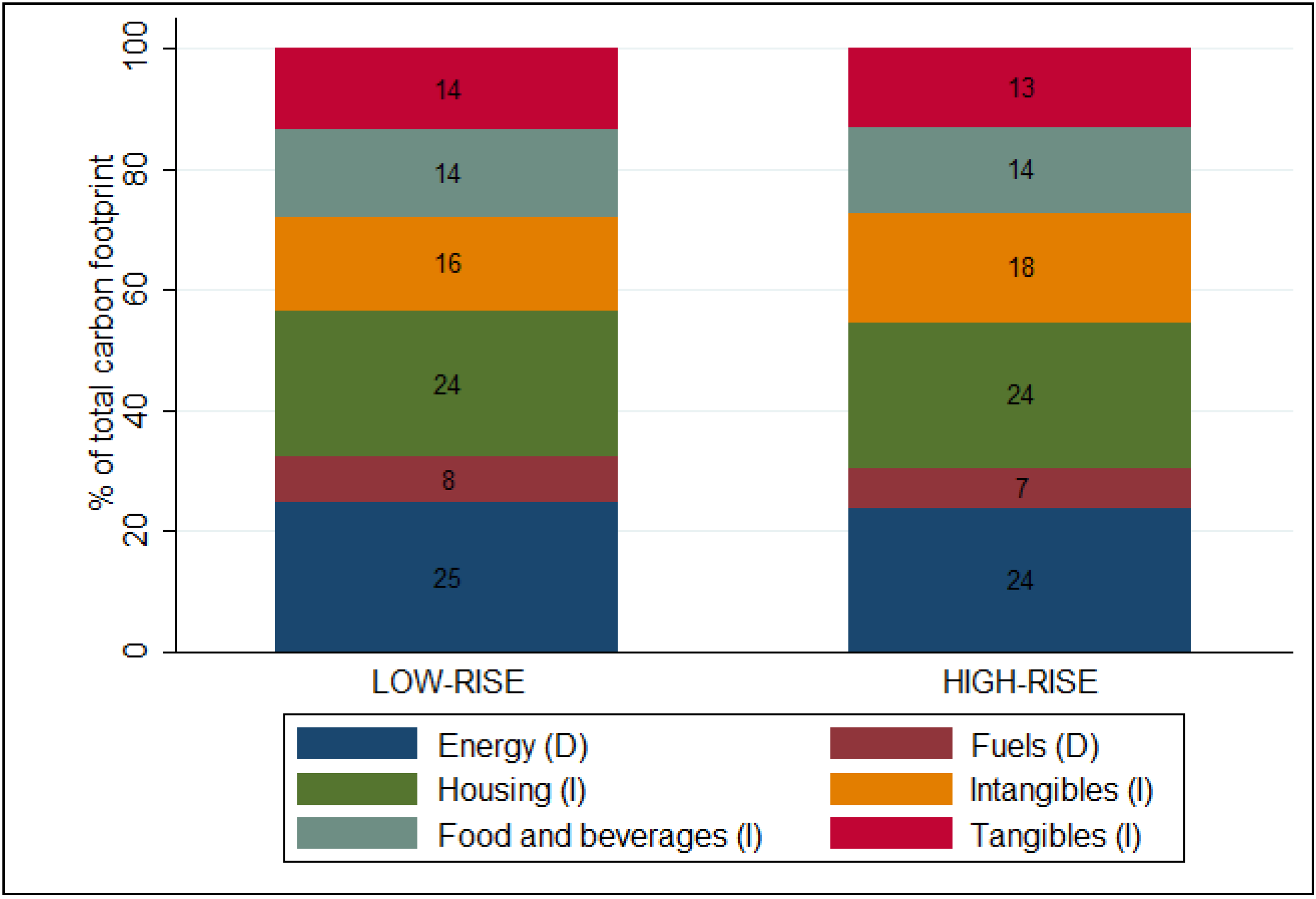
One of the most interesting observations about
Table 3 is that the absolute amount of greenhouse gases traceable to indirect products and services is relatively stable for both dweller types. Even though the mean disposable income of high-rise dwellers is clearly lower than that of low-rise dwellers, the differences in the amounts of emissions embodied in consumed products and services are fairly moderate. An equally interesting matter is the difference in GHG’s from fuel combustion for private driving: the difference between low-rise dwellers and those living in apartment houses is only 0.3 t despite the significant difference in the number of cars possessed on average. In order to further demonstrate the differences between dwellers living in different types of houses, we plot the percentage shares of home energy use, fuel, and emissions embodied in consumption of products and services. The results are presented in
Figure 1.
Figure 1.
Direct and indirect emission shares of carbon footprints for different dweller types.
Figure 1.
Direct and indirect emission shares of carbon footprints for different dweller types.
From
Figure 1, it can be concluded that there are no substantial differences in the relative sources of greenhouse gas emissions. Actually, all the sub-category shares are rather constant, and the differences are two percentage points at their largest.
Figure 1 also tells us that the emissions from indirect sources constitute approximately two-thirds of the total carbon footprints, whatever the type of dweller or dwelling. Energy and housing are the two most important sub-categories, alone covering half of the carbon footprint.
The next steps of our analysis are the regression analyses based on equation (2). When dummy variables are included, the chosen categories are compared to the reference group in parenthesis and the percentage difference in carbon footprints is approximated with p = 100(expβ-1) [
38]. First, we perform a univariate regression with logarithmic per-capita expenditure (regression 1). This is followed by multivariate regressions where dwelling type (regression 2) and household size (regression 3) are added to explanatory variables. The results are presented in
Table 4 below.
Table 4.
Results from regression models 1–3.
Table 4.
Results from regression models 1–3.
| Regression 1 | Regression 2 | Regression 3 |
|---|
| Variable | Estimate | SE | % effect | Estimate | SE | % effect | Estimate | SE | % effect |
|---|
| ln(E/capita) | 0.82*** | 0.02 | | 0.82*** | 0.02 | | 0.78*** | | |
| Dwelling (low-rise) |
| high-rise | | | | 0.01 | 0.03 | 1.0 | −0.03 | 0.03 | −3.3 |
| Dwellers (1 person) |
| 2 persons | | | | | | | −0.04 | 0.03 | −3.9 |
| more than 2 | | | | | | | −0.16*** | 0.03 | −15.2 |
| N | 568 | 568 | 568 |
| R2 | 0.7954 | 0.7955 | 0.8122 |
In the regression model 1 the average expenditure elasticity of an HMA resident is 0.82, meaning that a 10% increase in expenditure is related, on average, to an 8.2% increase in consumption-based greenhouse gas emissions. Thus, carbon footprints, even if due to indirect demand, can be defined to be due to normal goods with expenditure elasticity very close to unity. In regression 2, a dwelling-type dummy is added to the model. When compared to the reference group, that is low-rise dwellers, the estimate for high-rise gets a positive sign, meaning that, when controlling the amount of expenditure, the carbon footprints of high-rise dwellers are slightly larger than those of low-rise dwellers. Furthermore, when a household size variable is added to the model, the result turns around and the explanatory power of the model increases, as presented in regression model 3. Now, the footprints of high-rise dwellers are 3% lower than those of high-risers. The role of household size has a dominant role in the results and seems to have a clear effect on the carbon footprint of different dwelling types. In the literature, it has been suggested that there are so-called economies of scale in GHG’s, implying that the coefficients on bigger household sizes should be negative. Likewise, in our model the coefficients on household size get negative values, but the immediate impact is rather small, as the per-capita carbon footprints are only 4% smaller in a two-person household when compared to a single-person household. However, the coefficient is not statistically significant. The main efficiencies related to the size of a household become apparent in households with more than two members, their total per-capita carbon footprint being 15% smaller than that of single dwellers. The difference is statistically significant.
We also control the wealth level with income per capita. The results are presented in
Table 5 below. These income elasticity values are smaller than those for expenditure, but in general the results are in line with the results presented in
Table 4. The average income elasticity is 0.60, meaning that a 10% rise in per-capita disposable income is related to a 6% increase in carbon footprint. This is related to the role of saved income. It might also be possible that time restricts the growth in purchases when the disposable income increases above a certain level. Therefore, not enough free time is left for consuming the increasing income (see further e.g., [
33]). When income, instead of expenditure, is controlled, the effect of household size grows slightly. The effect of dwelling-type remains rather minor and statistically insignificant.
Table 5.
Results from regression models 4–6.
Table 5.
Results from regression models 4–6.
| | Regression 4 | Regression 5 | Regression 6 |
|---|
| Variable | Estimate | SE | % effect | Estimate | SE | % effect | Estimate | SE | % effect |
|---|
| ln(I/capita) | 0.60*** | 0.02 | | 0.60*** | 0.03 | | 0.56*** | 0.03 | |
| Dwelling (low-rise) |
| high-rise | | | | 0.02 | 0.03 | 2.5 | −0.03 | 0.03 | −2.9 |
| Dwellers (1 person) |
| 2 persons | | | | | | | −0.06 | 0.03 | −5.5 |
| more than 2 | | | | | | | −0.19*** | 0.04 | −17.6 |
| N | 568 | 568 | 568 |
| R2 | 0.6107 | 0.6112 | 0.6338 |
Finally, we analyze how direct and indirect emission shares behave when analyzed at the disaggregated level. We use the disaggregated per-capita emission and corresponding expenditure shares on the direct and indirect consumption categories instead of looking at the aggregated per-capita carbon footprints and expenditure levels. The models are of type (2), where the dependant variable is either the direct share of the carbon footprint (regression 7) or the indirect share of it (regression 8). Likewise, E is either direct or indirect per-capita expenditure, and dwelling-type and number of dwellers are used as dummy explanatory variables. The results are presented in
Table 6 below.
Table 6.
Results from regression models 7–8.
Table 6.
Results from regression models 7–8.
| | Regression 7 | Regression 8 |
|---|
| Variable | Estimate | SE | % effect | Estimate | SE | % effect |
|---|
| ln(Edirect/capita) | 0.76*** | 0.02 | | | | |
| ln(Eindirect/capita) | | | | 1.00*** | 0.01 | |
| Dwelling (low-rise) |
| high-rise | 0.01 | 0.03 | 0.9 | 0.04*** | 0.01 | 3.8 |
| Dwellers (1 person) |
| 2 persons | –0.14*** | 0.02 | –12.8 | 0.01 | 0.01 | 0.9 |
| more than 3 | –0.28*** | 0.02 | –24.6 | 0.01 | 0.01 | 0.7 |
| N | 568.00 | 568.00 |
| R2 | 0.8930 | 0.9590 |
Indirect emissions grow more steeply with expenditure level than do the direct ones. The direct expenditure elasticity is 0.76, meaning that a 10% rise in expenditure in housing energy and private driving is related to a growth of 7.6% in direct emissions. The corresponding figure for indirect emissions is 1, meaning that indirect GHGs grow linearly with expenditure on products and services. The dwelling type variable tells us that high-risers have on average 1% higher direct emissions when the amount of expenditure on direct categories is constant. The results is surprising as one could, based on earlier studies hypothesize lower direct emissions for high-rise dwellers. The tendency is similar for indirect GHGs, but the effect is more pronounced and statistically significant, which seems logical as the growing consumption could be expected to be directed more towards indirect consumption. Living in high-rise buildings leads here, on average, to 3.8% more of indirect emissions. Further, for direct emissions the number of dwellers plays a greater role than the type of dwelling, which, based on the earlier results above, also seems to be logical. Following the economies of scale hypothesis, those living in a two-person household are responsible, on average, for 13% less emissions per capita than those living alone. Noticeably, these economies of scale are not present when indirect emissions are explained in regression 8, which could be expected since the economies of scale typically have more direct influence on fixed costs (close to direct emissions here) than variable costs (close to indirect emissions here). Coefficients on household size carry positive signs but lack statistical significance. To sum up, it seems that there are factors related to high-rise lifestyle factors that can lead to higher indirect emissions. Direct emissions are more or less related to household size alone, and dwelling type’s role remains insignificant when the influence of household size is separated.
4. Discussion
4.1. The GHG Impacts of Urban Sprawl in HMA
The purpose of this paper was to explore how the phenomenon of urban sprawl is reflected in the GHG emissions of the residents of the HMA in Finland. For this purpose, the HMA was divided according to the housing type. We followed a premise that living in detached and semi-detached-houses can be typified as living in less dense sub-urban areas where the proximity to services is lower and public transportation networks are less efficient. This mode of living thus represents the features of sprawl that are considered the most negative in an intraurban context. Consumption-based GHG’s were assessed with the EE I-O LCA-model and further elaborated with a multivariate regression analysis.
Our results suggest that there are differences in the characteristics and lifestyles of metropolitan households by type of dwelling but some of these are not as explicitly evident when the actual GHG consequences are assessed. Our case area, the HMA, is a rather typical metropolis with a sprawling urban structure that, at the same time, has multiple positive features typical to metropolitan areas, the most important being its efficient public transportation network. Our results also highlight that, in order to make policies aimed to reduce GHG emissions, the structures of carbon footprints have to be kept in mind. The indirect part accounts for two-thirds of the footprint of a metropolitan dweller, and thus it should not be overlooked.
Looking at the averages, our results indicate that low-rise dwellers have higher carbon footprints than high-rise dwellers. The low-rise residents tend to be households with higher income, more children, and living in owner-occupied houses. However, the differences in the average amount of GHGs, both in absolute and relative terms, between the low-rise and high-rise dwellers are rather moderate compared with the figures from earlier literature. Many authors suggest that less-dense suburban living is approximately two times more energy- or GHG-intensive than inner-city living [
3,
4,
10,
34]. VandeWeghe and Kennedy [
5], for example, come up with a yearly difference of 1.3 t CO2-eq and smaller for those living in inner Toronto. Their result is rather close to our estimation of 1.8 t CO2-eq.
To some extent, our results also support earlier results stating that both the distances driven and the use of private vehicles increase in sprawling areas [
5,
6,
7]. However, according to our assessment these differences in emissions due to private transportation are remarkably small, indicating that private driving-related gains from higher density are moderate at best. This may also suggest that the better public transportation and better possibilities for walking and bicycling available for inner-city dwellers are not utilized up to their fullest potential. For example Kyttä
et al. [
35] suggest that Helsinki metropolitan dwellers rank smoothness of walking and bicycling very high, and indeed there has been attempts to make Helsinki more biker-friendly in recent years.
Our main results and key findings, however, were revealed when controlling for expenditure or income levels. Firstly, low-rise living is not unambiguously related to more GHG emissions than high-rise living. Actually, our regression models indicate that when expenditure or income levels are kept constant the high-rise dweller might produce equal or even slightly higher amounts of CHGs than the low-rise dweller. However, there was only one specification (regression 8) where the estimate for dwelling type had statistical significance. That told us that when the amount of expenditure on the indirect categories is kept constant the indirect footprints of high-rise dwellers are 4% higher than of those living in low-rise buildings. Secondly, household size, which in our case is usually larger in the low-rise living subset, seems to have a major effect on GHGs that are due to home energy and private driving. Economies of scale in household size are most unambiguous for households with at least three persons. Their per-capita carbon footprints are at least 15% smaller than those of people living alone, depending on the specification. The benefits of larger household size are most clearly seen when looking at the direct emissions, and the often-stated sharing of resources is not apparent when consumption of products and services alone is investigated. Thirdly, compared to household size, dwelling type is of minor importance.
Our analysis demonstrates that there are differences between low-rise and high-rise dwellers also within the metropolitan area. It is, however, worth asking if the differences between the two are to some extent over-emphasized, at least in the public debate? Our results suggest that the lifestyles within a metropolis and especially their GHG consequences do not vary as much as the background variables would suggest. On the one hand, it seems that those living in city centers make the most of consumption possibilities and less of the low-carbon possibilities available to them, and e.g., the potential for household-size scale benefits such as resource-sharing is not made use of. On the other hand, those living in sprawl areas are responsible for higher GHG emissions from housing energy and private driving, as is often stated.
However, even if we believe that our paper brings out important insights on how consumption patterns and their environmental consequences vary with building type, the disparities within each category cannot be neglected. Precisely, the less wealthy, whatever their housing conditions were, are not likely to generate great amounts of greenhouse gas emissions.
4.2. Limitations
One of the main methodological limitations of the paper is related to I-O assumption of homogenous prices. Even when a relatively limited area is considered, like the HMA in this paper, it is clear that the monetary quantity does not indicate the quality and even less the GHG consequences. The assumption probably overestimates greenhouse gas implications of the occupants of the wealthiest households, most of whom live in detached houses, and are likely to buy more expensive goods. The EE I-O method assumes that an item that costs 10 times more also causes 10 times more emissions. However, since the area of the study is relatively limited, it can be concluded that prices in sectors such as transportation and services are likely to be rather homogenous. For example, regional wage differences are not present.
There are also other assumptions than that of price homogeneity that are well-known weaknesses of EE I-O models [
21]. However, for example the bias related to high level of sector aggregation can be argued to be at a tolerable level. Su
et al. [
40] suggest that reliable estimates can be produced when the number of I-O sectors is at least 40. The EE I-O model utilized in this paper, therefore, meets this criterion with its 52 sectors. In addition, it has been pointed out that the errors tend to be at least partially negated when the final results are presented at a higher level of aggregation [
41].
Lacking exact spatial data on how households on our data are located, the results of this paper are based on a strong assumption about how the different building types are, on average, located within the Helsinki Metropolitan Area. The obvious problem is that there are high-rise buildings that are located at urban edge and vice versa. Furthermore, the distances to centers from low-rise areas vary, and low-rise areas located at farthest corners of HMA, like those in Kauniainen, represent sprawl more self-evidently than those located at some of the Helsinki’s suburbs. For example, for those living further afield from the city cores, the distances driven and the resulting emissions are likely to increase. However, we believe that our results give indications of general patterns since in the HMA apartment houses are almost invariably located in the centers of the HMA cities (Helsinki, Espoo, Vantaa, and Kauniainen), the share of apartment houses being highest in the capital (86%) [
36]. Furthermore, according to the most recent National Travel Survey, for the apartment dwellers in the HMA the average distance to the nearest public transport stop is 0.29 km, the corresponding figure for low-riser dwellers being 0.55 km [
37]. This indicates that our hypothesis is rather accurate.
It is worth noting that this paper restricts itself to a static analysis of the lifestyles with their GHG consequences. Our calculations are limited to consumption-based greenhouse gas emissions, referred as carbon footprints, and do not take into account e.g., the environmental pressure from increased land use and following changes in carbon stock [
48]. Often, the term urban sprawl refers to green field development, meaning new residential development taking place at the urban edge. Where sprawling areas replace former open or agricultural lands multiple environmental consequences arise (see e.g., [
49]). Furthermore, the expanding urban areas replace former green areas and also the CO
2 storage potential of these areas is lost or decreased. In addition, the carbon footprint comparisons in this study do not include the “carbon spike” related to construction of new infrastructure and buildings, be they located either in city centers or sprawling areas, even if this carbon spike is estimated to be quite substantial [
42,
43].
We use a rather limited amount of explanatory variables to explain carbon footprints. However, the literature includes a wide array of variables: e.g., education level, car ownership, and age [
23,
25]. However, none of these have been found to be of a similar importance as the level of expenditure and household size. Furthermore, analyses are often complicated by issues of multicollinearity and endogeneity.
Finally, we would like to highlight that our analysis is static and is not meant to be an analysis of change. Our results indicate an existence of an empirical relationship with given methodology in given point of time–it is unknown whether the results would recur e.g.
, in other countries. It must be kept in mind that the households who live in different environments are likely to differ in other ways as well. For example, it is impossible to assess to which extent the differences in carbon footprints are related to housing-types and not to households themselves. Living in the city core is also a lifestyle choice. For example, in the United States the liberal and environmentally-conscious prefer higher density areas with good public transport connections [
44] that can be considered to be an example of self-selection. This demonstrates the fact that people in green communities, for example, can have lower carbon footprints due to either selection or treatment effects. Here, treatment effect refers to a situation where the environment a person lives in has, for one reason or another, an effect on his or her behavior.
5. Conclusions
According to the study, the phenomenon of urban sprawl is, to some extent, revealed in the increased carbon footprints of suburban dwellers. However, our regression models indicate that when expenditure or income levels are controlled the suburban dweller might actually produce equal or even slightly lower amounts of GHGs than an inner-city dweller. More importantly, household size and the resulting economies of scale effects seem to have by far the greatest effect on carbon footprints.
Notwithstanding certain deficiencies that cause uncertainties in the calculations of carbon footprint and keeping in mind that our calculations do not take into account environmental consequences from increased land use and following changes in carbon stocks, some important policy implications arise. It would seem that the emissions from private driving decrease surprisingly moderately in the dense areas within the HMA, while living in an apartment house is related to lower emissions from housing energy consumption. Thus, controlling buildings’ energy efficiency would be of primary importance in preventing the negative effects of sprawl. On the other hand, either the available public transportation facilities may not be utilized up to their fullest potential or there still is room for improvement in the supply side. Using a private vehicle should be unnecessary in the densest areas. In addition, according to this study, the differences in indirect emissions from consumption of products and services are very small despite the large differences in disposable incomes. This suggests that proximity or other lifestyle-related factors may increase consumption of products and services and their indirect GHG consequences especially in city cores. All in all, consumption habits with their GHG consequences are surprisingly uniform across the HMA. Thus, instead of discussing only the differences between high-rise and low-rise areas, it would be essential to address why metropolitan areas have not yet fulfilled the great climate-change mitigation expectations imposed on them. The aim of the paper is not to deny the benefits of high-rise high-density policies but to discuss whether low-rise and not-as-high-density policies could and should act as complements to them. Our results suggests that if families that feel that they benefit from living in the suburban areas (there are also families that feel the opposite) moved to apartment houses, the final outcome, ceteris paribus, would remain almost the same at least when the viewpoint of consumption-based greenhouse gas emissions is taken. That is to say, an ideal metropolitan area would be an area where those living at the city core would not need a car and the benefits of closeness would stem from growing communality not from growing consumption. At the same time, those living in the suburban areas would live energy-efficiently and take an advantage of household size scale benefits as well as positive health effects of the proximity of green areas [
45]. Finally, this leads to a conclusion that actually more detailed information about different lifestyles and about the connections between the urban form and the lifestyle choices of households is needed in order to understand and mitigate the GHG consequences of urban sprawl. Sprawl is a complex phenomenon that is too often over-simplified to a single factor such as private driving.


