Analysis and Projection of the Relationship between Industrial Structure and Land Use Structure in China

Abstract

Based on the computable general equilibrium (CGE) modelling method, this research analyzes the relationship between industrial structure and land use structure in China. The results show that our model is feasible, and the simulation results are of a certain stability. Under the scenario analysis and projection of the relationship between the industrial structure and land use structure of the thirty-one provinces in China from 2010 to 2020, the proportions of secondary and tertiary industry in each province have been increasing; correspondingly, the proportion of agriculture has been decreasing. This means that the industrial structure of China is changing. As for land use, in general, the trend is similar to the industrial structure changes. The transformation of the structure of industrial development and land use has driven economic structure changes in China. The economic structure has an inclination to transform from agriculture to both secondary and tertiary industry. Along with industrial transformation, the cultivated land in China shows a trend of continuous decline. Empirical analysis results indicate that a decrease of cultivated land is acceptable under the scenario of economic growth in the next ten years. This shows a possibility that the economic efficiency of land use for cultivation and business services will decline, and more attention ought to be paid to increasing the economic efficiency of land use.

1. Introduction

Land is the foundation of human survival, as well as the basic material for social production [1]. Land use is a process in which humans transform natural land to meet the demands of socio-economic development. Various types of land use are formed in that structural transformation process. It directly affects the human activities of using and planning their living environment [2]. Land use structure is the proportional land use that reflects the pattern of socioeconomic development in an economic structure [3]. The industrial structure represents the interrelationships and the interdependence of sectoral production. Their proportional relationships among sectors systematically demonstrate the integrity of the interaction of the social production process and its proportional changes in the reformation of social production [4]. In other words, it shows the composition of each sector in the economic structure [5]. Grasping the trend of land use change and its impacts on the improvement of sectoral production efficiency for economic development is of unusual significance.

Industrial structure and land use structure are closely related. Industrial structure is the structure of the proportions of various industries in a specific region. Land use structure is the structure of the shares of different types of land use for various industries in a specific region. Because land is the fundamental factor for production activities, the adjustment of the economic industrial structure will inevitably change the demand for land use and, thus, alter the land use structure [6]. Kuznets (1955) said that the proportion for the industrial and service sectors would increase until the economy developed to a certain level. The production factors of agriculture would be transferred to secondary and tertiary industry [7]. The investment-oriented and policy-oriented adjustment of the industrial structure can drive the reallocation of production inputs. In return, land use structure interacts with the structural changes of industrial production. Meanwhile, economic structure is the structure based on the industrial structure under the designed scenarios. Government strategic policy on sustainable development somehow reshapes this interaction process for strategically guaranteeing the balance between economic growth and resource utilization, which guides the adjustments of industrial structure and land use structure.

The computable general equilibrium (CGE) model can quantitatively describe the relationships and interdependencies among components of various economies within a complex social system [8,9,10]. Theoretically, this model reflects the structure of a bundle of systematic equilibriums through a market mechanism to depict both the supply and demand of commodities and services in a unit pricing system. Moreover, by giving a well-structured depiction of physical land use, the application of the CGE model has been extended to analyze land use analysis based on traditional market economy theory.

In this paper, based on an analysis of the current pattern of land use in China, we examined the relationship between industrial structure and land use structure in the thirty-one provinces (Note: Taiwan, Hong Kong and Macao have not been included, due to a lack of statistical data). This will help us research future decision making in the optimization of land use structure and contribute to further reformation of industrial development under advanced land management planning. This model and data description will be presented in the following Section 2. Thereafter, empirical analysis and simulation results will be given in Section 3. At the end of this paper, we provide the conclusions of this research and a discussion of further research directions.

2. Model and Data

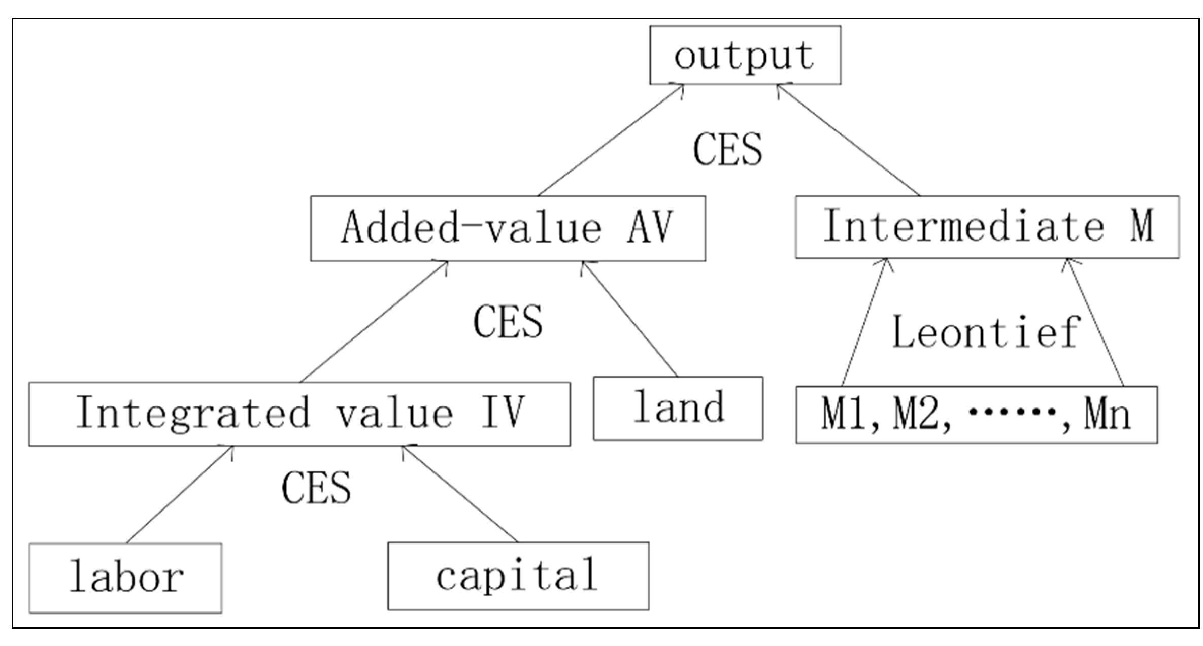
2.1. Multi-Regional CGE Model

Based on multi-regional CGE modelling, the constraints of land use were introduced into the potential productivity process. Through a mathematic operation research approach by using time series data of land use and its demand changes, a robust land use prediction model was built. In the following sections, three nested production functions are combined with the coordinated environmental sustainability (CES) production function and Leontief production function, which will be introduced into the CGE model, as in Figure 1.

Figure 1. Nested production function structure. CES, coordinated environmental sustainability.

Figure 1. Nested production function structure. CES, coordinated environmental sustainability.

The third level of production functions includes capital and labor, which represents an integrated value. The second level includes two production levels. One is the integration of labor and capital and land, which are converted to added value through the transaction of the CES production function. The other one is the combination of intermediate inputs through the transaction of the Leontief production function. The function at each level of production functions as follows:

The first level of nested CES final demand:

$$Q_i=A_i\cdot {\left(\mathrm{\eta }\cdot A{V}_i^{-{\rho }_i}+(1-\mathrm{\eta })M_i^{-{\rho }_i}\right)}^{-\frac{1}{\begin{array}{l}{\text{ρ}}_i\\ \end{array}}}$$

(1)

The second level of nested CES added value:

$$A{V}_i=A_i^{AV}\cdot {\left({\mathrm{\delta }}_i^{AV}I{V}_i^{-{\rho }_i^{AV}}+\left(1-{\mathrm{\delta }}_i^{AV}\right)LN{D}_i^{-{\rho }_i^{AV}}\right)}^{-\frac{1}{{\text{ρ}}_i^{IV}}}$$

(2)

The second level of nested CES intermediate inputs:

$$M_i=\min \left\{a_1\cdot M_1,a_2\cdot M_2,\text{L},a_n\cdot M_n\right\}=a_j\cdot M_j$$

(3)

The third level of nested CES intermediate inputs of labor and capital:

$$I{V}_i=A_i^{IV}\cdot {\left({\mathrm{\delta }}_i^{IV}\cdot {L_i}^{-{\rho }_i^{IV}}+(1-{\mathrm{\delta }}_i^{IV}){K_i}^{-{\rho }_i^{IV}}\right)}^{-\frac{1}{\begin{array}{l}{\rho }_i^{IV}\\ \end{array}}}$$

(4)

The production process is a process to pursue maximum profit (or the minimum of the production cost). When profits reach the maximum level (or the cost reaches the minimum level), each factor input is the factor demand. Except the above input-output production function, solving the objective function also requires introducing the price relationships. Under this condition of the nest CES structure, if the objective function is the cost minimum function, an objective function of a certain good will be represented as follows:

$$Min. C_i=P_i^{AV}\cdot A{V}_i+P_i^M\cdot M_i$$

(5)

The relevant price relationships are:

$$p_i^Q\cdot Q_i=P_i^{AV}\cdot A{V}_i+p_i^M\cdot M_i$$

(6)

$${p_i}^{AV}\cdot A{V}_i=P_i^{IV}\cdot I{V}_i+p_i^{LND}\cdot LN{D}_i$$

(7)

$$p_i^{IV}\cdot IV=p_i^L\cdot L_i+p_i^K\cdot K_i$$

(8)

$$p_i^M\cdot M_i={\displaystyle \sum _i^j{p}^{X_i}}\cdot M_i$$

(9)

where and below,

• i is the sector of crop, wool, other agriculture, secondary industry, construction and service industry;
• j is the other sectors of i;
• t, is the year from 2000–2020;
• r is a region of the31 provinces in China;
• l is the other regions of r;
• d is the land use type of crop, wool, other agriculture, secondary industry, construction and service industry.

2.1.1. Constraints of Land Use

According to the restrictions of land use and land planning, the constraints of land use are shown in the following equations.

The sum of the total area of land use for each sector in each province is smaller or equal to the total area of land in each province:

$${\displaystyle \sum _{i=1}^{6}XLN{D}_{i,r}}\le XLND\_I{I}_r$$

(10)

where $i$ is the sector and $r$ is the region.

Land supply is not smaller than the inventory in the planning period:

$$XLN{D}_{1,r}\ge XLND{P}_{crop,r}$$

(11)

where $XLND{P}_{crop,r}$ is the inventory in the planning period.

Land supply in each region is not beyond the upper bound of the inventory in the planning period:

$$XLN{D}_{4,r}+XLN{D}_{5,r}+XLN{D}_{6,r}\le XLND{P}_{cons,r}$$

(12)

where $XLND{P}_{cons,r}$ is the upper bound of the inventory in the planning period.

In addition, in the simulation process, with respect to other land use types, built-up land is special. In the short term, the built-up area will not shrink; in other words, the current built-up area will not be smaller than it was in the last year, no matter how much the outputs increase in the area.

$$XconsLN{D}_t\ge XconsLN{D}_{t-1}$$

(13)

2.1.2. Agricultural Production Impact Function

Apparently, each sector can be influenced by a combination of factor inputs and land use changes. Relatively speaking, agricultural production can be influenced by land use changes, which are more than the proportional changes in sectoral production. Usually, agricultural production is directly and fundamentally affected by land use changes, and this kind of influence will easily transfer to the secondary and tertiary sectors, sequentially affecting the whole economic system. Therefore, we introduce the agricultural production impact function for comprehensively assessing the impact factors of the agriculture sector. We assume this might influence the secondary and tertiary sectors by using the dynamic multi-regional CGE model.

Agricultural production usually is influenced by many impact factors, such as natural hazards, human factor intervention, production planning reformation and technology innovation. Among those factors, natural disasters have the most impact on agricultural production. In 2013, agricultural production had a loss of 125.6 billion CNY due to natural disasters. Therefore, we focus on how much impact natural hazards have on land use, because this mainly induces agricultural production loss, in order to analyze the possible impacts on the secondary and tertiary industries in the next ten years.

The impact factor of natural disasters is represented by the ratio of the production loss area over the total area of land use in the following equation:

$${\text{λ}}_{i,t}=\frac{D{Q}_{i,t}}{LN{D}_{i,t}}$$

(14)

where ${\text{λ}}_{i,t}$ is the coefficient of the i type of land suffering from natural hazards, $D{Q}_{i,t}$ is the area of the i type of land with production loss in the t year and $LN{D}_{i,t}$ is the total area of the i type of land in the t year.

It is easy to figure out that natural hazards mainly influence cultivated land productivity and, then, influence the cultivated land supply. Moreover, natural hazards have less impact on other types of land use, such as built-up land, unused land, and so forth, and could be ignored. Thereby, when cultivated land converts to other types of land use, we consider this as $D{Q}_{i,t}=0$. Thus, the natural hazard impact factor on each type of land use is as follows:

$${\text{λ}}_{i,t}=\{\begin{array}{l}\frac{D{Q}_{i,t}}{LN{D}_{i,t}},i=1,2,3\\ 0,i=4,5,6\end{array}$$

(15)

Natural hazards mainly have impacts on productive cultivated land, woodland and grassland. Thereafter, there are three different levels to describe the impact of natural hazards on agricultural lands, which represent disaster, harmed and lost. Disaster represents less than 10 percent of the expected agricultural productivity being lost. Harmed land represents about 30 percent, but less than 70 percent of the expected agricultural productivity being lost. Lost land represents more than 70 percent of the expected agricultural productivity being lost. Therefore, the total amount of agricultural productivity loss due to natural hazards is computable in the following equations:

Total area of agricultural productivity loss = flood impacted land + hailstorm impacted land + frost impacted land + drought impacted land + hurricane impacted land = (flood impacted land *0.1 + flood impacted land * 0.3 + flood impacted land * 0.7) + (hailstorm impacted land * 0.1 + hailstorm impacted land * 0.3 + hailstorm impacted land * 0.7) + (frost impacted land * 0.1 + frost impacted land * 0.3 + frost impacted land * 0.7) + (drought impacted land * 0.1 + drought impacted land * 0.3 + drought impacted land * 0.7) + (hurricane impacted land * 0.1 + hurricane impacted land * 0.3 + hurricane impacted land * 0.7).

The above conceptual equation is represented by the mathematical equation as follows:

$$D{Q}_{i,t}=fl{Q}_{i,t}+wi{Q}_{i,t}+lt{Q}_{i,t}+dr{Q}_{i,t}+ty{Q}_{i,t}$$

(16)

where,

$$fl{Q}_{i,t}=flS{Q}_{i,t}\cdot 0.1+flC{Q}_{i,t}\cdot 0.3+flJ{Q}_{i,t}\cdot 0.7$$

$$wi{Q}_{i,t}=wiS{Q}_{i,t}\cdot 0.1+wiC{Q}_{i,t}\cdot 0.3+wiJ{Q}_{i,t}\cdot 0.7$$

$$lt{Q}_{i,t}=ltS{Q}_{i,t}\cdot 0.1+ltC{Q}_{i,t}\cdot 0.3+ltJ{Q}_{i,t}\cdot 0.7$$

$$dr{Q}_{i,t}=drS{Q}_{i,t}\cdot 0.1+drC{Q}_{i,t}\cdot 0.3+drJ{Q}_{i,t}\cdot 0.7$$

$$ty{Q}_{i,t}=tyS{Q}_{i,t}\cdot 0.1+tyC{Q}_{i,t}\cdot 0.3+tyJ{Q}_{i,t}\cdot 0.7$$

A natural disaster happens suddenly, which may bring about huge, unpredictable loss. Based on the 2000–2011 historical data, which is produced by Jin Qing [11], we use the average of that value to predict the impacts of a natural disaster on land use. According to Equation (16), we obtain the data for the total area of land suffering from a natural disaster in each province of China from 2000 to 2011. Sequentially, according to Equation (15), the impact factor of natural disasters on land use and changes in each province of China from 2000 to 2011 can be calculated. Finally, the average of the impact factor of natural disasters on land use and changes in each province of China from 2000 to 2011 are listed in Table 1, which can be used for forecasting natural disaster impacts on land use and changes in each province of China.

Table 1. Impact factors of natural disasters on land use in each province of China * (10⁴ hm²).

Region	Disaster Area	Agricultural Area	Natural Disaster Impact Factor	Region	Disaster Area	Agricultural Area	Natural Disaster Impact Factor
China	1,749.89	15,463.58	0.1132	Henan	92.19	1,335.98	0.0690
Beijing	6.30	34.20	0.1842	Hubei	100.55	735.50	0.1367
Tianjing	8.60	52.28	0.1645	Hunan	133.04	778.99	0.1708
Hebei	125.33	893.51	0.1403	Guangdong	59.60	493.24	0.1208
Shanxi	58.22	390.05	0.1493	Guangxi	46.76	629.99	0.0742
Inner Mongolia	96.55	588.70	0.164	Hainan	11.10	86.33	0.1286
Liaoning	62.06	380.92	0.1629	Chongqing	49.31	346.71	0.1422
Jilin	52.14	468.77	0.1112	Sichuan	71.56	956.46	0.0748
Heilongjiang	128.92	985.84	0.1308	Guizhou	44.31	464.54	0.0954
Shanghai	1.29	47.67	0.027	Yunnan	51.82	581.31	0.0891
Jiangsu	24.30	779.79	0.0312	Tibet	1.31	23.29	0.0562
Zhejiang	23.68	306.45	0.0773	Shaanxi	74.20	419.83	0.1767
Anhui	43.45	899.76	0.0483	Gansu	47.47	364.99	0.1301
Fujian	30.85	266.14	0.1159	Qinghai	12.65	49.43	0.2559
Jiangxi	43.02	535.51	0.0803	Ningxia	16.44	114.79	0.1432
Shandong	209.13	1,104.78	0.1893	Xinjiang	23.73	347.83	0.0682

* Note: natural disasters include: flood, hailstorm, frost, drought and hurricanes; data from China Statistic Yearbook 2001–2012 and China Agricultural Statistic Yearbook 2001–2012.

Table 1. Impact factors of natural disasters on land use in each province of China * (10⁴ hm²).

Region	Disaster Area	Agricultural Area	Natural Disaster Impact Factor	Region	Disaster Area	Agricultural Area	Natural Disaster Impact Factor
China	1,749.89	15,463.58	0.1132	Henan	92.19	1,335.98	0.0690
Beijing	6.30	34.20	0.1842	Hubei	100.55	735.50	0.1367
Tianjing	8.60	52.28	0.1645	Hunan	133.04	778.99	0.1708
Hebei	125.33	893.51	0.1403	Guangdong	59.60	493.24	0.1208
Shanxi	58.22	390.05	0.1493	Guangxi	46.76	629.99	0.0742
Inner Mongolia	96.55	588.70	0.164	Hainan	11.10	86.33	0.1286
Liaoning	62.06	380.92	0.1629	Chongqing	49.31	346.71	0.1422
Jilin	52.14	468.77	0.1112	Sichuan	71.56	956.46	0.0748
Heilongjiang	128.92	985.84	0.1308	Guizhou	44.31	464.54	0.0954
Shanghai	1.29	47.67	0.027	Yunnan	51.82	581.31	0.0891
Jiangsu	24.30	779.79	0.0312	Tibet	1.31	23.29	0.0562
Zhejiang	23.68	306.45	0.0773	Shaanxi	74.20	419.83	0.1767
Anhui	43.45	899.76	0.0483	Gansu	47.47	364.99	0.1301
Fujian	30.85	266.14	0.1159	Qinghai	12.65	49.43	0.2559
Jiangxi	43.02	535.51	0.0803	Ningxia	16.44	114.79	0.1432
Shandong	209.13	1,104.78	0.1893	Xinjiang	23.73	347.83	0.0682

* Note: natural disasters include: flood, hailstorm, frost, drought and hurricanes; data from China Statistic Yearbook 2001–2012 and China Agricultural Statistic Yearbook 2001–2012.

2.1.3. Land Demand Prediction Model

Here, the growth rate of land is equal to the growth rate of production; then, the growth of land demand can be represented as follows:

$$A\_LN{D}_{i,d}=\frac{A\_Q_{i,d}}{A\_TF{P}_{i,d}+1}$$

(17)

where $A\_LN{D}_{i,d}$ is the growth rate of land demand, $A\_Q_{i,d}$ is the growth rate of production and $A\_TF{P}_{i,d}$ is the growth rate of other factor inputs.

Under the constraints of the total number of each type of land, the minimum deviance of the land demand and its satisfaction coefficient in a certain period are set up in the objective function.

$$\min {{\displaystyle \sum _i\left(\frac{RD{L}_{i,d,\Delta t}}{MD{L}_{i,d,\Delta t}}-{\text{ξ}}_{i,d,\Delta t-1}\right)}}^2$$

(18)

$$s.t.{\displaystyle \sum _{i}RD{L}_{i,d,\Delta t}}=0, i=1,2,\cdots ,6;d=1,2,\cdots ,31$$

(19)

where $RD{L}_{i,d,\Delta t}$ is actual changes of land at time t, $MD{L}_{i,d,\Delta t}$ is land demand at time t and ${\text{ξ}}_{i,d,\Delta t-1}$ is the satisfaction coefficient in the previous time t − 1, which is equal to the ratio of land use changes divided by the land demand in previous time t − 1, where the previous land use changes are calculated by the LaGrange multiplier method within the prediction model as follows:

(1)

Auxiliary function:

$$\Phi ={\displaystyle \sum _{i=1}^6{\left(\frac{RD{L}_{i,d,\Delta t}}{MD{L}_{i,d,\Delta t}}-{\text{ξ}}_{i,d,\Delta t-1}\right)}^2}+\text{λ}\cdot {\displaystyle \sum _{i=1}^{6}RD{L}_{i,d,\Delta t}}$$

(20)

(2)

Take the derivative of $RD{L}_{i,d,\Delta t}$, and solve for the static point of $\text{Φ}$:

$$\frac{\partial \text{Φ}}{\partial RD{L}_{i,d,\Delta t}}=\frac{2}{MD{L}_{i,d,\Delta t}}\cdot \left(\frac{RD{L}_{i,d,\Delta t}}{MD{L}_{i,d,\Delta t}}-{\text{ξ}}_{i,d,\Delta t-1}\right)+\text{λ}=0$$

(21)

(3)

According to Equation (21), the relationship of $RD{L}_{i,d,\Delta t}$ and $\text{λ}$ can be derived:

$$RD{L}_{i,d,\Delta t}=\frac{MD{L}_{i,d,\Delta t}^2}{2}\cdot \left(\frac{{\text{ξ}}_{i,d,\Delta t}}{MD{L}_{i,d,\Delta t}}-\text{λ}\right)$$

(22)

(4)

Plug Equation (22) into the equation ${\displaystyle \sum _{i=1}^{6}RD{L}_{i,d,\Delta t}}=0$ to get $\text{λ}$ as the following equation:

$$\text{λ}=-\frac{{\displaystyle \sum _{i=1}^6{\text{ξ}}_{i,d,\Delta t-1}\cdot MD{L}_{i,d,\Delta t}}}{{\displaystyle \sum _{i=1}^{6}MD{L^2}_{i,d,\Delta t}}}$$

(23)

(5)

According to Equations (22) and (23), the equation is reached:

$$RD{L}_{i,d,\Delta t}=\frac{MD{L}_{i,d,\Delta t}^2}{2}\cdot \left(\frac{{\text{ξ}}_{i,d,\Delta t}}{MD{L}_{i,d,\Delta t}}+\frac{{\displaystyle \sum _{i=1}^6{\text{ξ}}_{i,d,\Delta t-1}\cdot MD{L}_{i,d,\Delta t}}}{{\displaystyle \sum _{i=1}^{6}MD{L^2}_{i,d,\Delta t}}}\right)$$

(24)

2.2. CES Production Function Elastic Parameter Estimation

Bayesian estimation of Markov chain Monte Carlo methods (MCMC) [12] is used for estimating the elasticity of the CES production function, to renew the original data of the parameters and to implement dynamic parameter inputs. The parameter estimation is in Table 2 and Table 3. All of the numbers for the constant elasticity of substitution are generated by the Bayesian estimation method, which are all inside of the range of the CES production function from 0.1 to 2.5 [13]. Therefore, the elasticities used in this research are acceptable as parameter inputs to the multi-regional CGE model (see the Appendix).

Table 2. The elasticity of the substitution between the land and the integrated value of labor and capital in each sector.

Sector	Elasticity of Substitution	Sector	Elasticity of Substitution
Planting	1.99	Manufacturing	0.86
Dairy	1.99	Construction	0.26
Other Agriculture	1.99	Tertiary	0.26

Table 2. The elasticity of the substitution between the land and the integrated value of labor and capital in each sector.

Sector	Elasticity of Substitution	Sector	Elasticity of Substitution
Planting	1.99	Manufacturing	0.86
Dairy	1.99	Construction	0.26
Other Agriculture	1.99	Tertiary	0.26

Table 3. The elasticity of substitution between added value and intermediate inputs in each sector.

Sector	Elasticity of Substitution	Sector	Elasticity of Substitution
Planting	0.34	Manufacturing	2.01
Dairy	0.34	Construction	2.02
Other Agriculture	0.34	Tertiary	1.01

Table 3. The elasticity of substitution between added value and intermediate inputs in each sector.

Sector	Elasticity of Substitution	Sector	Elasticity of Substitution
Planting	0.34	Manufacturing	2.01
Dairy	0.34	Construction	2.02
Other Agriculture	0.34	Tertiary	1.01

2.3. Sensitivity Analysis

Assessing the CGE model usually requires examining whether the tiny changes of some generally key parameters have impacts on the optimum solution. Therefore, sensitivity analysis is used to test the robustness of the optimum solution.

Assume the key parameter as $\mathrm{\theta }$; the optimum solution of the function is $F\left(X,\mathrm{\theta }\right)=0$ is $X^{*}$. With respect to one of the neighborhoods ${\rm O}\left(\mathrm{\theta }-\Delta \theta ,\mathrm{\theta }+\Delta \mathrm{\theta }\right)$ of $\mathrm{\theta }$, if $\exists {\mathrm{\theta }}^{\prime }\in {\rm O}\left(\mathrm{\theta }-\Delta \mathrm{\theta },\mathrm{\theta }+\Delta \mathrm{\theta }\right)$, which let $F\left(X,{\mathrm{\theta }}^{\prime }\right)=0$ have the optimum solution at $X^{*}ˈ$, then $\forall \text{ε}>0$ and $\left|X^{*}ˈ-X^{*}\right|<\text{ε}$. Here, we call the model robust. Theoretically, a smaller $\text{ε}$ is better. However, actually, as long as $\left|X^{*}ˈ-X^{*}\right|$ stays in a certain acceptable range, we can also claim that the model is robust.

It is necessary to perform numerous extractions in the neighborhoods to statistically describe the average and variance of the model or the given confidence interval [14], so that we reach a reliable conclusion.

The elasticity of substitution of the CES production function is distributed in (0.1, 2.5). Thereby, when doing sensitivity analysis on that, we extract the elasticity of substitution from the average distribution in (0.1, 2.5). Therefore, in the simulation process, the elasticity of substitution is randomly selected from (0.1, 2.5). Computing program of the model run 1000-times under this scenario of two percent of the growth in all factor inputs, and then, the elasticity of substitution of the endogenous variables in the CGE model within the 95% confidence interval is derived in Table 4 (See Appendix).

Table 4. Sensitivity analysis results *.

Variable	Average	SD	Lower Bound of CI	Upper Bound of CI
ES1	1.919	0.032	1.892	2.033
ES2	0.842	0.013	0.678	0.902
ES3	0.258	0.201	0.296	0.287
ES4	0.262	0.450	0.264	0.313
ES5	0.341	0.023	0.32	0.381
ES6	1.988	0.056	1.932	2.012
ES7	2.101	0.023	1.998	2.174
ES8	1.001	0.220	0.999	1.035
GDP1	0.030	0.044	0.027	0.035
GDP2	0.025	0.022	0.024	0.027
GDP3	0.011	0.051	0.012	0.017
GDP4	0.015	0.033	0.014	0.018
GDP5	0.012	0.310	0.01	0.016
GDP6	0.016	0.256	0.015	0.018
GDP7	0.013	0.345	0.012	0.017
GDP8	0.015	0.617	0.009	0.02
GDP9	0.031	0.240	0.026	0.033
GDP10	0.028	0.025	0.026	0.031
GDP11	0.027	0.052	0.026	0.034
GDP12	0.014	0.038	0.013	0.016
GDP13	0.020	0.029	0.016	0.024
GDP14	0.013	0.515	0.014	0.017
GDP15	0.015	0.362	0.014	0.018
GDP16	0.012	0.028	0.013	0.016
GDP17	0.013	0.053	0.012	0.018
GDP18	0.015	0.036	0.017	0.021
GDP19	0.033	0.05	0.032	0.038
GDP20	0.013	0.2	0.009	0.015
GDP21	0.008	0.045	0.009	0.012
GDP22	0.012	0.03	0.011	0.019
GDP23	0.012	0.03	0.01	0.018
GDP24	0.007	0.01	0.007	0.01
GDP25	0.007	0.02	0.006	0.012
GDP26	0.004	0.03	0.003	0.008
GDP27	0.012	0.03	0.011	0.015
GDP28	0.009	0.03	0.009	0.011
GDP29	0.010	0.01	0.009	0.013
GDP30	0.009	0.02	0.008	0.014
GDP31	0.011	0.03	0.009	0.016

* Note: ES1 to ES8 sequentially represent the elasticity of substitution at the first level and second level of the CES production function, respectively, in agriculture, manufacturing sectors, construction sectors and tertiary industry; GDP1 to GDP31 represent changes in the rate of GDP in the 31 provinces of China, respectively.

Table 4. Sensitivity analysis results *.

Variable	Average	SD	Lower Bound of CI	Upper Bound of CI
ES1	1.919	0.032	1.892	2.033
ES2	0.842	0.013	0.678	0.902
ES3	0.258	0.201	0.296	0.287
ES4	0.262	0.450	0.264	0.313
ES5	0.341	0.023	0.32	0.381
ES6	1.988	0.056	1.932	2.012
ES7	2.101	0.023	1.998	2.174
ES8	1.001	0.220	0.999	1.035
GDP1	0.030	0.044	0.027	0.035
GDP2	0.025	0.022	0.024	0.027
GDP3	0.011	0.051	0.012	0.017
GDP4	0.015	0.033	0.014	0.018
GDP5	0.012	0.310	0.01	0.016
GDP6	0.016	0.256	0.015	0.018
GDP7	0.013	0.345	0.012	0.017
GDP8	0.015	0.617	0.009	0.02
GDP9	0.031	0.240	0.026	0.033
GDP10	0.028	0.025	0.026	0.031
GDP11	0.027	0.052	0.026	0.034
GDP12	0.014	0.038	0.013	0.016
GDP13	0.020	0.029	0.016	0.024
GDP14	0.013	0.515	0.014	0.017
GDP15	0.015	0.362	0.014	0.018
GDP16	0.012	0.028	0.013	0.016
GDP17	0.013	0.053	0.012	0.018
GDP18	0.015	0.036	0.017	0.021
GDP19	0.033	0.05	0.032	0.038
GDP20	0.013	0.2	0.009	0.015
GDP21	0.008	0.045	0.009	0.012
GDP22	0.012	0.03	0.011	0.019
GDP23	0.012	0.03	0.01	0.018
GDP24	0.007	0.01	0.007	0.01
GDP25	0.007	0.02	0.006	0.012
GDP26	0.004	0.03	0.003	0.008
GDP27	0.012	0.03	0.011	0.015
GDP28	0.009	0.03	0.009	0.011
GDP29	0.010	0.01	0.009	0.013
GDP30	0.009	0.02	0.008	0.014
GDP31	0.011	0.03	0.009	0.016

* Note: ES1 to ES8 sequentially represent the elasticity of substitution at the first level and second level of the CES production function, respectively, in agriculture, manufacturing sectors, construction sectors and tertiary industry; GDP1 to GDP31 represent changes in the rate of GDP in the 31 provinces of China, respectively.

From the simulation results, under the condition of two percent growth in all production factor inputs, the growth rate of GPD in the 31 provinces of China is about 0.7 to 3.4 percent, with the confidence interval at 0.5 to 4 percent. This illustrates that the fluctuation of the elasticity of substitution has a small impact on the simulation results; therefore, the simulation results are robust.

3. Empirical Analysis and Results

3.1. Scenario Design

According to the draft of the 13th Five-Year Plan of China Development reported by the National Development and Reform Commission, three scenarios were designed for analyzing the relationships between industrial structure and land use structure, which were named the business-as-usual (BAU) scenario, the rapid economic growth (REG) scenario and the coordinated environmental sustainability (CES) scenario.

Here, we chose the population growth rate, investment growth rate and total factor productivity (TFP) growth rate as the variables to set the scenarios for future socio-economic development (Table 5). Firstly, the BAU scenario is set according to the forecast of the economic development in China, which could act as the baseline to be compared with other scenarios. In this scenario, the rate of labor force growth is obtained based on the projection of population and workforce age. The investment growth rate is set to decrease with the increase of economic development. We assume that the growth rate of TFP will continue this pattern and remain around 2% in 2011–2020 [15]. On this basis, we further develop the CES and REG scenarios according to the opportunities and challenges that China might be facing, together with the environmental conservation policies in the process of development. In the CES scenario, we conventionally assume that the population growth pressure and investment growth rate are both slightly lower than that in the baseline scenario [16]. In the REG scenario, we conventionally assume that the population growth rate is relatively high, that the investment growth rate is higher than that in the BAU scenario and that the TFP growth rate is higher than that in the BAU scenario.

Table 5. Socio-economic development scenarios in China, 2011–2020. BAU, business-as-usual; TFP, total factor productivity; REG, rapid economic growth.

Scenario	Indicator	Growth Rate (%)
BAU	Labor	0.28
	Capital	8.40
	TFP	2.00
CES	Labor	0.30
	Capital	8.05
	TFP	1.90
REG	Labor	0.25
	Capital	8.70
	TFP	2.10

Table 5. Socio-economic development scenarios in China, 2011–2020. BAU, business-as-usual; TFP, total factor productivity; REG, rapid economic growth.

Scenario	Indicator	Growth Rate (%)
BAU	Labor	0.28
	Capital	8.40
	TFP	2.00
CES	Labor	0.30
	Capital	8.05
	TFP	1.90
REG	Labor	0.25
	Capital	8.70
	TFP	2.10

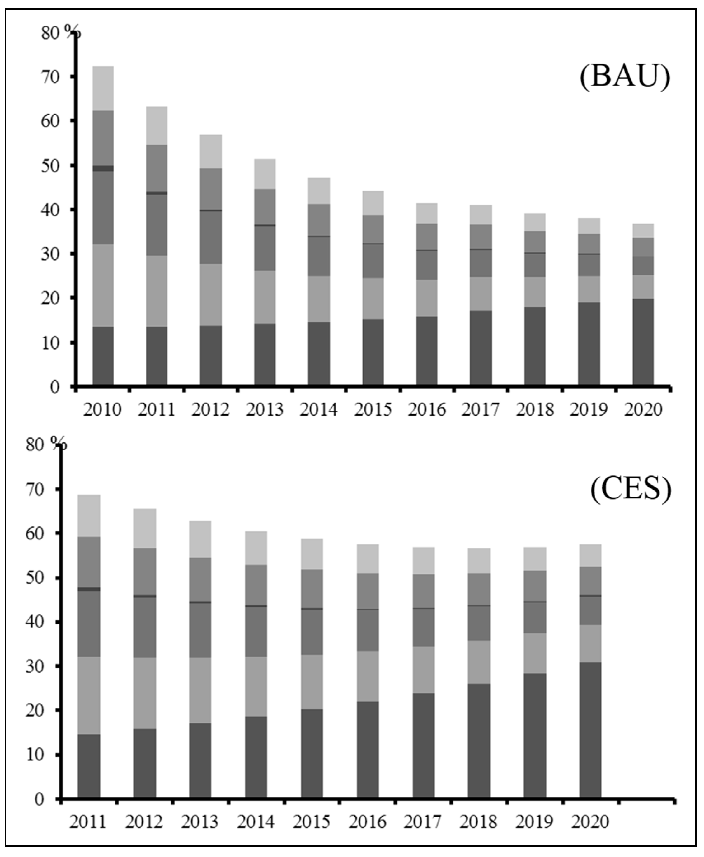
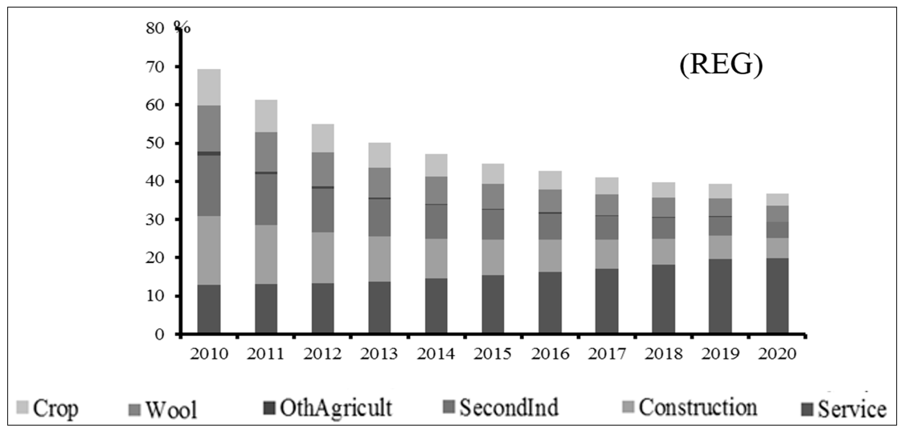
3.2. Industrial Structure Change Projection

3.2.1. Industrial Structure Change in China

By applying the CGE model, the change rate of the output value of various industries in the thirty-one provinces was simulated under three scenarios in China. Based on the output value and the simulated change rate in 2010, the output values in 2010–2020 were generated. Additionally, the output values’ contribution was calculated as shown in Figure 2.

Figure 2. Analysis results of industrial structure change in China from 2010 to 2020 under scenarios of BAU, CES, and REG.

Figure 2. Analysis results of industrial structure change in China from 2010 to 2020 under scenarios of BAU, CES, and REG.

The simulated results showed that, in the three scenarios in 2010–2020, the secondary and service industries take the largest proportion. The changing trend of the industrial structure is similar (Table 2), with agriculture and the service industry transferring to secondary industry. The proportion of agriculture is shrinking, while the trend is stable. The proportion of the secondary industry shows an obvious increase. The proportions of the construction and service industry are decreasing.

The change rate of the industrial structure in the next ten years in China was calculated based on the proportion of various industries from 2010 to 2020 (Table 6). The proportion of the secondary industry under all three scenarios shows an increasing trend, while other industries are decreasing, with the service industry decreasing the most. Among the three scenarios, in REG, all industries, other than the secondary one, decreased the most. The range of BAU is smaller than that in REG, while the CES possesses the lowest range.

Under the BAU scenario, the proportion of the crop planting industry will decrease by 1.63% from 2010 to 2020, while animal husbandry will decrease by 1.89%; the other agricultural sectors will decrease by 0.73%; secondary industry will decrease by 23.63%; the construction and service industries will respectively decrease by 3.67% and 15.71%. Under the CES scenario, crop planting, animal husbandry and other agriculture will respectively decrease by 1.52%, 1.81% and 0.73%; while the secondary industry will increase by 22.63%. The construction and service industries will respectively decrease by 3.6% and 14.98%. Under the REG scenario, crop planting, animal husbandry and other agriculture will respectively decrease by 1.71%, 1.95% and 0.76%; while the secondary industry will increase by 24.54%, and the construction and service industry will respectively decrease by 3.76% and 16.37% from 2010 to 2020.

Table 6. Change rate of industrial structure in China under three scenarios, 2010–2020 (%).

BAU
Time	Crop	Wool	Other Agriculture	Secondary Industry	Construction	Service Industry
2010–2011	−0.08	−0.13	−0.06	1.87	−0.44	−1.16
2011–2012	−0.10	−0.15	−0.06	2.00	−0.43	−1.26
2012–2013	−0.12	−0.16	−0.07	2.12	−0.42	−1.35
2013–2014	−0.13	−0.18	−0.07	2.24	−0.41	−1.45
2014–2015	−0.15	−0.19	−0.08	2.36	−0.39	−1.55
2015–2016	−0.17	−0.20	−0.08	2.47	−0.37	−1.64
2016–2017	−0.19	−0.21	−0.08	2.56	−0.35	−1.73
2017–2018	−0.21	−0.22	−0.08	2.63	−0.32	−1.80
2018–2019	−0.23	−0.22	−0.08	2.68	−0.29	−1.86
2019–2020	−0.25	−0.22	−0.08	2.71	−0.25	−1.92
CES
Time	Crop	Wool	Other Agriculture	Secondary Industry	Construction	Service Industry
2010–2011	−0.08	−0.12	−0.06	1.80	−0.42	−1.12
2011–2012	−0.09	−0.14	−0.06	1.92	−0.42	−1.20
2012–2013	−0.11	−0.16	−0.07	2.03	−0.41	−1.29
2013–2014	−0.13	−0.17	−0.07	2.14	−0.40	−1.38
2014–2015	−0.14	−0.18	−0.07	2.25	−0.38	−1.47
2015–2016	−0.16	−0.20	−0.07	2.35	−0.36	−1.56
2016–2017	−0.18	−0.20	−0.08	2.44	−0.34	−1.64
2017–2018	−0.20	−0.21	−0.08	2.51	−0.31	−1.72
2018–2019	−0.21	−0.21	−0.08	2.56	−0.28	−1.78
2019–2020	−0.22	−0.22	−0.09	2.63	−0.28	−1.82
REG
Time	Crop	Wool	Other Agriculture	Secondary Industry	Construction	Service Industry
2010–2011	−0.09	−0.13	−0.06	1.94	−0.45	−1.20
2011–2012	−0.10	−0.15	−0.07	2.07	−0.45	−1.30
2012–2013	−0.12	−0.17	−0.07	2.20	−0.44	−1.40
2013–2014	−0.14	−0.19	−0.07	2.33	−0.42	−1.51
2014–2015	−0.16	−0.20	−0.08	2.46	−0.41	−1.61
2015–2016	−0.18	−0.21	−0.08	2.57	−0.38	−1.71
2016–2017	−0.20	−0.22	−0.08	2.66	−0.35	−1.80
2017–2018	−0.22	−0.23	−0.08	2.74	−0.32	−1.89
2018–2019	−0.24	−0.23	−0.08	2.78	−0.29	−1.94
2019–2020	−0.26	−0.22	−0.08	2.80	−0.25	−1.99

Table 6. Change rate of industrial structure in China under three scenarios, 2010–2020 (%).

BAU
Time	Crop	Wool	Other Agriculture	Secondary Industry	Construction	Service Industry
2010–2011	−0.08	−0.13	−0.06	1.87	−0.44	−1.16
2011–2012	−0.10	−0.15	−0.06	2.00	−0.43	−1.26
2012–2013	−0.12	−0.16	−0.07	2.12	−0.42	−1.35
2013–2014	−0.13	−0.18	−0.07	2.24	−0.41	−1.45
2014–2015	−0.15	−0.19	−0.08	2.36	−0.39	−1.55
2015–2016	−0.17	−0.20	−0.08	2.47	−0.37	−1.64
2016–2017	−0.19	−0.21	−0.08	2.56	−0.35	−1.73
2017–2018	−0.21	−0.22	−0.08	2.63	−0.32	−1.80
2018–2019	−0.23	−0.22	−0.08	2.68	−0.29	−1.86
2019–2020	−0.25	−0.22	−0.08	2.71	−0.25	−1.92
CES
Time	Crop	Wool	Other Agriculture	Secondary Industry	Construction	Service Industry
2010–2011	−0.08	−0.12	−0.06	1.80	−0.42	−1.12
2011–2012	−0.09	−0.14	−0.06	1.92	−0.42	−1.20
2012–2013	−0.11	−0.16	−0.07	2.03	−0.41	−1.29
2013–2014	−0.13	−0.17	−0.07	2.14	−0.40	−1.38
2014–2015	−0.14	−0.18	−0.07	2.25	−0.38	−1.47
2015–2016	−0.16	−0.20	−0.07	2.35	−0.36	−1.56
2016–2017	−0.18	−0.20	−0.08	2.44	−0.34	−1.64
2017–2018	−0.20	−0.21	−0.08	2.51	−0.31	−1.72
2018–2019	−0.21	−0.21	−0.08	2.56	−0.28	−1.78
2019–2020	−0.22	−0.22	−0.09	2.63	−0.28	−1.82
REG
Time	Crop	Wool	Other Agriculture	Secondary Industry	Construction	Service Industry
2010–2011	−0.09	−0.13	−0.06	1.94	−0.45	−1.20
2011–2012	−0.10	−0.15	−0.07	2.07	−0.45	−1.30
2012–2013	−0.12	−0.17	−0.07	2.20	−0.44	−1.40
2013–2014	−0.14	−0.19	−0.07	2.33	−0.42	−1.51
2014–2015	−0.16	−0.20	−0.08	2.46	−0.41	−1.61
2015–2016	−0.18	−0.21	−0.08	2.57	−0.38	−1.71
2016–2017	−0.20	−0.22	−0.08	2.66	−0.35	−1.80
2017–2018	−0.22	−0.23	−0.08	2.74	−0.32	−1.89
2018–2019	−0.24	−0.23	−0.08	2.78	−0.29	−1.94
2019–2020	−0.26	−0.22	−0.08	2.80	−0.25	−1.99

3.2.2. Industrial Structure Change in Each Province

Based on the analysis of the industrial structure changes in China, we further select Beijing, Guangdong, Heilongjiang, Hubei, Qinghai and Jiangxi as the representatives of the thirty-one provinces, to analyze the industrial structure. (Figure 3).

In 2010, under all three scenarios, the secondary and service industry are in an absolutely advantageous state. Among the six provinces, the proportion of service industry in Beijing is the largest. The secondary and service industries in Guangdong account for more than 80%. In Heilongjiang, the crop planting industry takes the largest proportion. The proportion of crop planting industry in Hubei is relatively higher, while the secondary industry proportion is lower, and the proportion for the service industry is higher than that of other provinces other than Beijing. In Qinghai province, the proportion for animal husbandry is relatively higher, while in Jiangxi province, the proportion of other agriculture and construction industries are higher.

Figure 3. Scenario analysis results of industrial structure change in the six typical provinces from 2010 to 2020 under scenarios of BAU, CES, and REG.

Figure 3. Scenario analysis results of industrial structure change in the six typical provinces from 2010 to 2020 under scenarios of BAU, CES, and REG.

In 2020, under the three scenarios, the secondary and service industries are still in an absolutely advantageous state. Compared with 2010, in every province, there are obvious increases in the proportion of the secondary industry, obvious decreases in the service industry, and slight increases in crop planting and slight decreases in animal husbandry, other agriculture and the construction industry.

During 2010 to 2020, the change rates of the industrial structure are different under different scenarios. (Table 7). Under the BAU and REG scenarios, the proportions of secondary industry are all increasing in the six provinces, but the proportions of other industries are decreasing. Under the CES scenario, the proportions for crop planting and secondary industry are increasing, while the proportions for other industries are decreasing.

Table 7. Change rate of industrial structure in six provinces of China under three scenarios, 2010–2020 (%).

BAU
Region	Crop	Wool	Other Agriculture	Secondary Industry	Construction	Service Industry
Beijing	−0.06	−0.21	−0.05	25.16	−3.06	−21.78
Guangdong	−0.91	−0.85	−0.69	21.11	−2.16	−16.49
Heilongjiang	−2.50	−2.65	−0.44	23.05	−3.53	−13.93
Hubei	−2.13	−2.56	−1.20	26.34	−3.73	−16.72
Qinghai	−1.75	−3.68	−0.10	29.95	−6.23	−18.20
Jiangxi	−2.39	−2.78	−1.99	28.05	−6.78	−14.11
CES
Region	Crop	Wool	Other Agriculture	Secondary Industry	Construction	Service Industry
Beijing	1.71	−0.33	−0.08	37.91	−4.05	−35.17
Guangdong	4.56	−1.19	−0.93	24.34	−2.67	−24.10
Heilongjiang	11.70	−3.85	−0.61	18.73	−4.40	−21.57
Hubei	14.89	−4.02	−1.77	22.57	−4.76	−26.92
Qinghai	5.77	−4.98	−0.13	31.30	−7.45	−24.52
Jiangxi	11.39	−4.11	−2.79	25.07	−8.43	−21.14
REG
Region	Crop	Wool	Other agriculture	Secondary Industry	Construction	Service Industry
Beijing	−0.06	−0.22	−0.05	26.48	−3.14	−23.00
Guangdong	−0.95	−0.88	−0.71	21.93	−2.21	−17.18
Heilongjiang	−2.61	−2.74	−0.45	23.91	−3.61	−14.49
Hubei	−2.25	−2.66	−1.24	27.42	−3.82	−17.45
Qinghai	−1.83	−3.80	−0.10	30.92	−6.35	−18.83
Jiangxi	−2.51	−2.88	−2.05	29.05	−6.93	−14.67

Table 7. Change rate of industrial structure in six provinces of China under three scenarios, 2010–2020 (%).

BAU
Region	Crop	Wool	Other Agriculture	Secondary Industry	Construction	Service Industry
Beijing	−0.06	−0.21	−0.05	25.16	−3.06	−21.78
Guangdong	−0.91	−0.85	−0.69	21.11	−2.16	−16.49
Heilongjiang	−2.50	−2.65	−0.44	23.05	−3.53	−13.93
Hubei	−2.13	−2.56	−1.20	26.34	−3.73	−16.72
Qinghai	−1.75	−3.68	−0.10	29.95	−6.23	−18.20
Jiangxi	−2.39	−2.78	−1.99	28.05	−6.78	−14.11
CES
Region	Crop	Wool	Other Agriculture	Secondary Industry	Construction	Service Industry
Beijing	1.71	−0.33	−0.08	37.91	−4.05	−35.17
Guangdong	4.56	−1.19	−0.93	24.34	−2.67	−24.10
Heilongjiang	11.70	−3.85	−0.61	18.73	−4.40	−21.57
Hubei	14.89	−4.02	−1.77	22.57	−4.76	−26.92
Qinghai	5.77	−4.98	−0.13	31.30	−7.45	−24.52
Jiangxi	11.39	−4.11	−2.79	25.07	−8.43	−21.14
REG
Region	Crop	Wool	Other agriculture	Secondary Industry	Construction	Service Industry
Beijing	−0.06	−0.22	−0.05	26.48	−3.14	−23.00
Guangdong	−0.95	−0.88	−0.71	21.93	−2.21	−17.18
Heilongjiang	−2.61	−2.74	−0.45	23.91	−3.61	−14.49
Hubei	−2.25	−2.66	−1.24	27.42	−3.82	−17.45
Qinghai	−1.83	−3.80	−0.10	30.92	−6.35	−18.83
Jiangxi	−2.51	−2.88	−2.05	29.05	−6.93	−14.67

Under the BAU scenario, the growth rate of secondary industry in Qinghai is the highest by 29.95 percent among all provinces. The recession rates for crop planting, animal husbandry and other agriculture in Beijing are the lowest. While in Heilongjiang, Qinghai and Jiangxi, crop planting, animal husbandry and other agriculture will decrease the most. In Jiangxi, the construction industry will decrease the most at 6.78%; while in Beijing, the service industry will decrease the most at 21.78%. Under the CES scenario, Hubei and Beijing will have the largest increase in crop planting and secondary industry. Qinghai and Jiangxi will have the largest decrease in animal husbandry and other agriculture. Jiangxi and Beijing will have the largest increase in the construction and service industries. Under the REG scenario, the secondary industry will increase the most in Qinghai at 30.92%, and the least increase will be in Guangdong at 21.93%. The provinces that will have the largest decrease in crop planting, animal husbandry and other agriculture remain in a similar situation under the BAU scenario, and those provinces that have the largest decrease in the construction and service industry remain in a similar situation under the CES scenario.

From the above analysis, we can see that the distinguished structures of the advantageous industries in each province have been influenced by different scenarios. Under the CES scenario, the secondary industry will increase relatively faster, but will decrease faster in the advantageous industries. Under the REG scenario, the myth of the advantageous industries will fade with an increasing trend in the secondary industry.

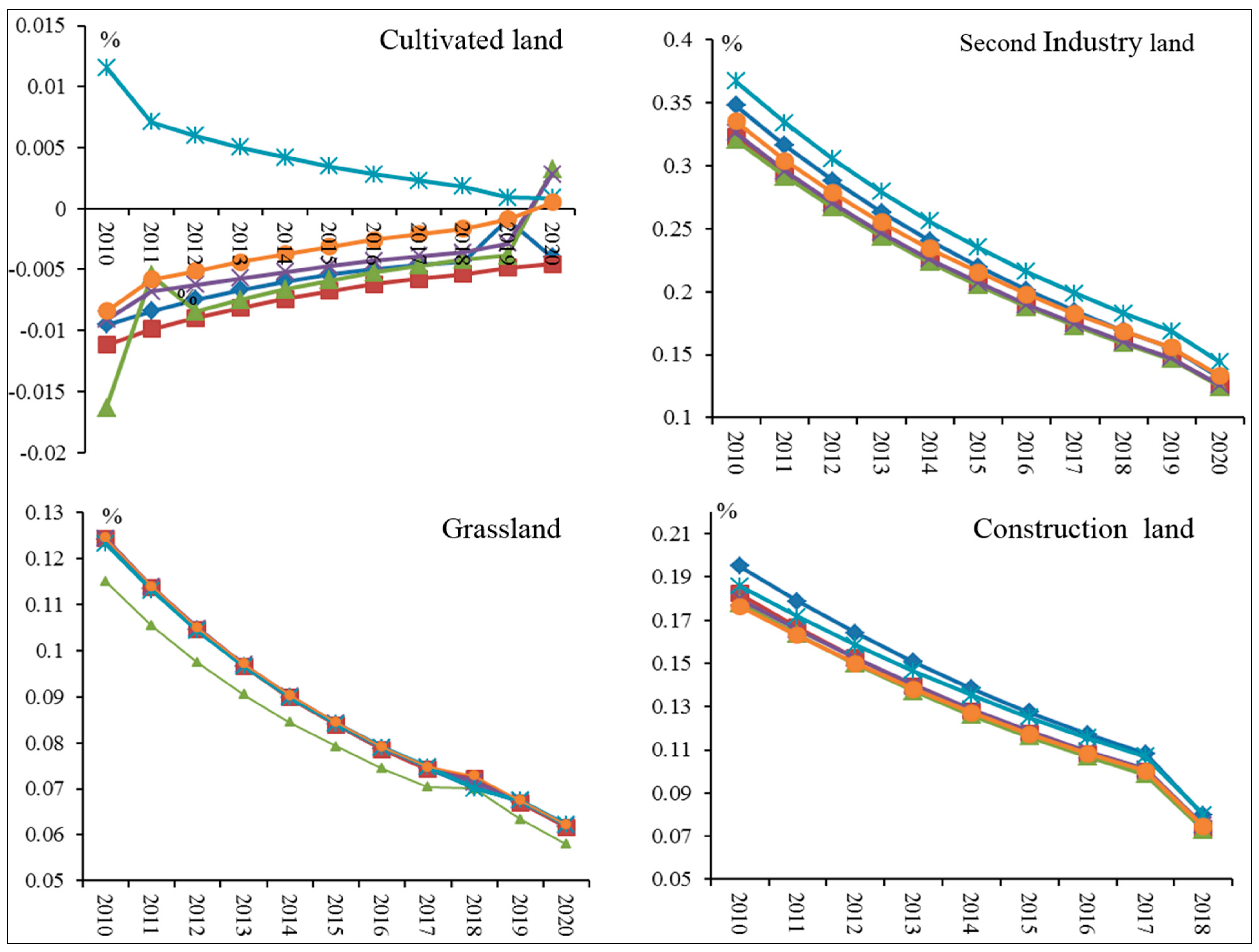
3.3. Land Use Change Projection

3.3.1. Land Use Changes in China

In this land use prediction model, we calculated land use changes in 31 provinces in China. By adding up the total amount of changes in each province, we analyzed the characteristics of the trend of land use changes in the next ten years.

The three scenarios show a similar trend with respectively changing variance. Land use under the REG scenario shows the largest variance compared to the other two scenarios; the second largest is under the BAU scenario, and the lowest variance is under the CES scenario. From 2010 to 2020, the growth rate of land use for manufacturing and urban construction is decreasing, while the growth rate for cultivated land, grassland and other land use for agriculture is decreasing. From Figure 4, until 2020, the land use structure will remain balanced, since increasing land uses can compensate for decreasing land uses.

Figure 4. Land use changes in China from 2010 to 2020 based on three scenarios of BAU, CES and REG.

Figure 4. Land use changes in China from 2010 to 2020 based on three scenarios of BAU, CES and REG.

From the Figure 5, we see that cultivated land, grassland and land use for other agriculture are increasing, while land use for manufacturing and urban construction are decreasing year by year. However, each type of land use is decreasing in different amounts.

Figure 5. The trends of six types of land use under the three scenarios in China 2010–2020.

Figure 5. The trends of six types of land use under the three scenarios in China 2010–2020.

From 2010 to 2020, cultivated land use will shrink at a decreasing rate. Under the economic growth-oriented scenario, cultivated land will shrink relatively more than under the other two scenarios, which is about 119.3 thousand ha. Next is under BAU, which is about 113.9 thousand ha. Under the CES scenario, cultivated land use will shrink 108.3 thousand ha. Grassland changes with the same trend as cultivated land. Under the REG scenario, it will shrink the most: about 147.6 thousand ha. Under the BAU scenario, this number is about 139.1 thousand ha. Under the CES scenario, it will shrink 129.7 thousand ha. Other land uses for agriculture are also decreasing. Under the same sequence of scenarios, it will decrease 14.3 thousand ha, 13.6 thousand ha and 12.9 thousand ha, respectively. However, the land use for manufacturing is annually increasing, but with a decreasing growth rate. It will increase 54.2 thousand ha, 51.3 thousand ha and 48.3 thousand ha, respectively, under the REG scenario, BAU scenario and CES scenario. The land use for urban construction will also increase 137 thousand ha, 129.5 thousand ha and 121.4 thousand ha under the same sequence of scenarios. The land use for other built-up areas will also increase, even more than the land use for manufacturing, about 89.9 thousand ha, 85.8 thousand ha and 81.3 thousand ha, respectively.

According to the national land use plan in 2006–2020, until 2010, total cultivated land in China was about 121 million ha, total land use for urban construction was about 0.3374 million ha and, until 2020, the total amount of cultivated land will not be less than 120.33 million ha; the total land use for urban construction will reach 37.24 million ha [17]. Based on this modified CGE model, we predict the total land use for cultivation and urban construction under the three scenarios from 2010 to 2020 in Table 8. Based on Table 8 and the constraint data of land use for cultivation and urban construction in 2010, we predict the total land use for cultivation and urban construction in 2020 in Table 9.

Table 8. Changes of land use for cultivation and urban construction under the three scenarios in China 2010–2020 (10 thousand ha).

Scenarios	Cultivation	Urban Construction
BAU	−11.39	26.66
CES	−10.83	25.09
REG	−11.93	28.11

Table 8. Changes of land use for cultivation and urban construction under the three scenarios in China 2010–2020 (10 thousand ha).

Scenarios	Cultivation	Urban Construction
BAU	−11.39	26.66
CES	−10.83	25.09
REG	−11.93	28.11

Table 9. Estimated land use for cultivation and urban construction under the three scenarios in China 2010–2020 (10 thousand ha).

Scenarios	Cultivation	Urban Construction
BAU	12,108.61	3400.66
CES	12,109.17	3399.09
REG	12,108.07	3402.11

Table 9. Estimated land use for cultivation and urban construction under the three scenarios in China 2010–2020 (10 thousand ha).

Scenarios	Cultivation	Urban Construction
BAU	12,108.61	3400.66
CES	12,109.17	3399.09
REG	12,108.07	3402.11

Until 2020, cultivated land will be over 120.33 million ha, so that the target for cultivated land protection will be reached; while the target of 37.24 million ha for urban construction will not be reached under the three scenarios. Therefore, although cultivated land will decrease, it is in the acceptable range. Until 2020, food security will be protected under the total area of cultivated land at 1.8 billion mu. With economic growth, urban construction will require more land, but its expansion will be acceptable, as well, and still have the possibility of rising.

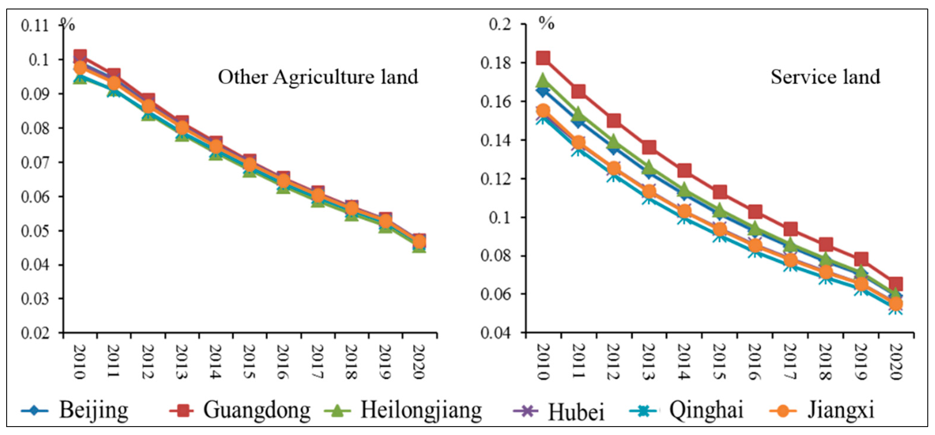
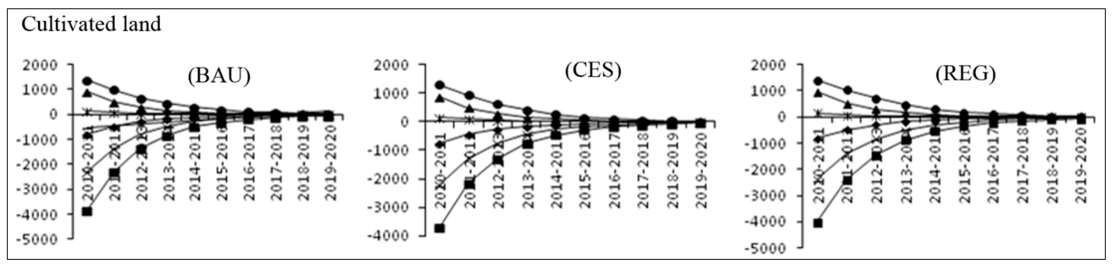
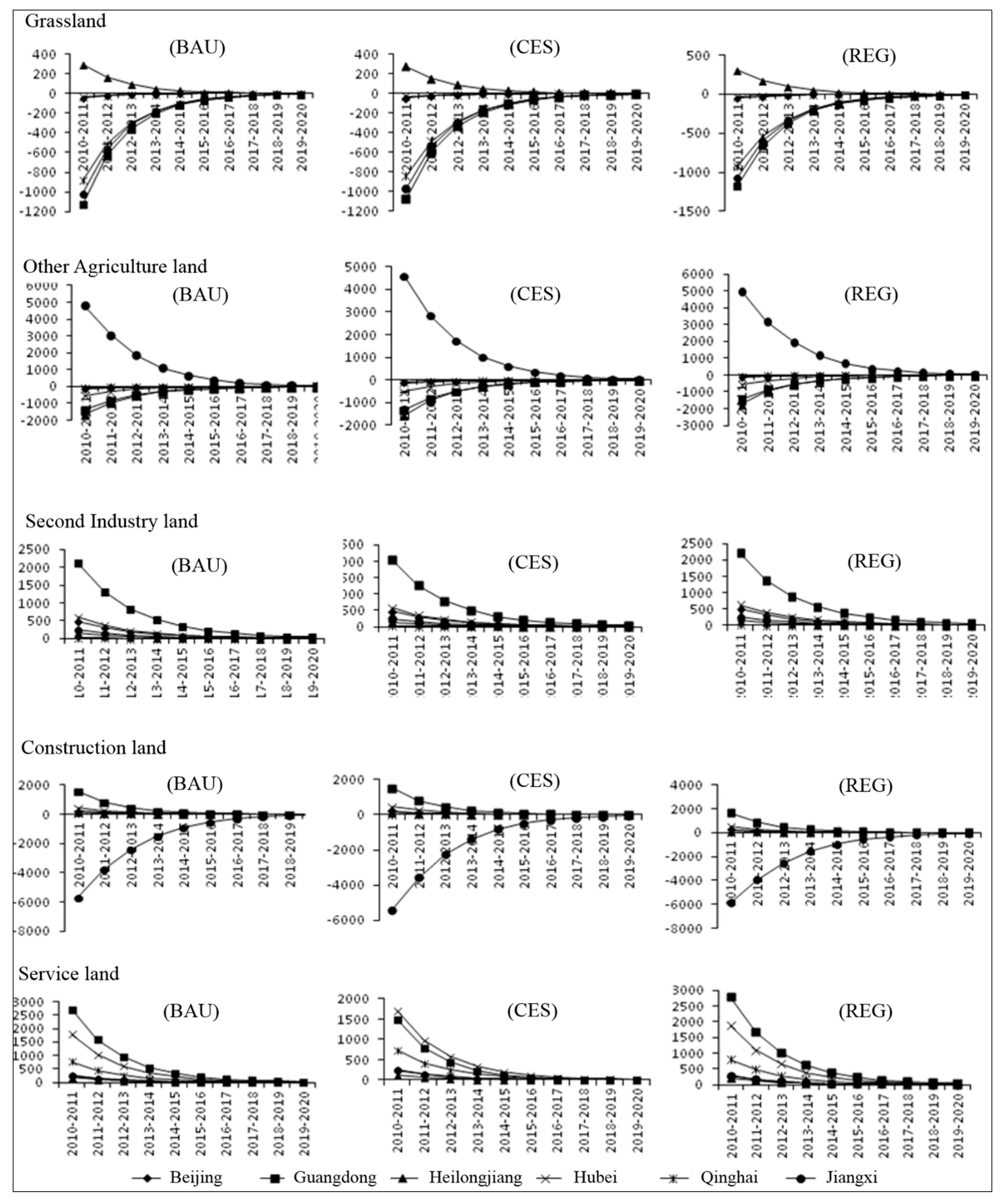
3.3.2. Land Use in Each Province

We selected Beijing, Guangdong, Heilongjiang, Hubei, Qinghai and Jiangxi to analyze the trend of land use changes from 2010 to 2020 in China.

Figure 6 shows that the six types of land use changes in the six provinces will decrease during 2010–2020. Until 2020, land use in China will tend to be stable. Sequentially, under the REG scenario, the fundamental scenario and the CES scenario, the variance of the changes of land use is sequentially smaller than the previous scenario. From 2010 to 2020, six types of land use changes will decrease, until 2020, becoming relatively stable. Specifically, cultivated land in Heilongjiang, Qinghai and Jiangxi is increasing, while it will decrease in Beijing, Guangdong and Hubei. Meanwhile, Guangdong will be the one with the greatest decreases. Grassland in Heilongjiang will increase, while it will decrease in Beijing, Guangdong, Hubei, Qinghai and Jiangxi. Meanwhile, Guangdong will be the one with the greatest decrease again. Other land use for agriculture in Jiangxi will increase, while it will decrease in the other five provinces, and Heilongjiang will be the one with the greatest decrease. Land use for manufacturing will increase in all six provinces, but with a decreasing growth rate. Meanwhile, Guangdong will be the one with the greatest increase, but Qinghai will be the one with the lowest increase. Land use for urban construction will increase in the provinces, except Jiangxi, and Guangdong will be the one with the greatest increase. Other land for built-up areas will increase in all six provinces; Guangdong will be the one with the greatest increase, and Heilongjiang will be the one with the lowest increase.

Figure 6. Trends of six types of land use changes in six provinces in China 2010–2020.

Figure 6. Trends of six types of land use changes in six provinces in China 2010–2020.

From 2010 to 2020, as shown in Figure 7, land use changes in six provinces will be most influenced under the REG scenario, but the least under the CES scenario. Specifically, cultivated land will increase with the greatest amount in Jiangxi province, about 4360.86 ha, 4130.36 ha and 3869.73 ha, which are respectively under the REG scenario, fundamental scenario and CES scenario. Cultivated land will decrease the greatest amount in Guangdong province, about 10,138.04 ha, 9649.81 ha and 9122.97 ha, which are respectively under REG, BAU and CES. Grassland will only increase in Heilongjiang, about 697.11 ha, 663.85 ha and 629.22 ha, which are respectively under REG, BAU and CES. Grassland will decrease the greatest amount in Guangdong, about 2725.29 ha, 2594.73 ha and 2458.49 ha, which are respectively under REG, BAU and CES. Other land use for agriculture will only increase in Jiangxi, about 12,972.94 ha, 12,344.04 ha and 11,666.72 ha, which are respectively under REG, BAU and CES. Other land use for agriculture will decrease the greatest in Heilongjiang, about 4072.94 ha, 3886.75 ha and 3688.24 ha, which are respectively under REG, BAU and CES. Land use for manufacturing will increase in all six province. Guangdong will increase the greatest, about 6098.39 ha, 5777.86 ha and 5435.54 ha, which are respectively under the economic growth-oriented scenario, the fundamental scenario and environmentally-oriented scenario, while Qinghai will increase least, about 55.09 ha, 52.09 ha and 48.9 ha, which are respectively under REG, BAU and CES. Land use for urban construction will increase the most in Guangdong province, about 3543.28 ha, 3401.9 ha and 3245.29 ha, which are respectively under REG, BAU and CES. Comparing the other five provinces, other land use for built-up areas will increase the most in Guangdong, as well, about 6972.64 ha, 6647.32 ha and 6293.85 ha, which are respectively under REG, BAU and CES.

Figure 7. Trends of six types of land use changes in six provinces in China under three scenarios 2010–2020.

Figure 7. Trends of six types of land use changes in six provinces in China under three scenarios 2010–2020.

3.4. Relationship Analysis of Future Industrial Structure and Land Use Structure

Based on the land use amount in 2010 and the land use change from 2010 to 2020, the land use amount for 2020 was calculated. Then, based on the land use amount for 2010 and 2020, the land use structure of 2010 and 2020 and the structural change during 2010–2020 were calculated. Based on the data in the three scenarios, the change in the industrial structure and land use structure in China from 2010 to 2020 was analyzed. (Table 10).

Table 10. Industrial structure and land use structure change under three scenarios in China, 2010–2020 (Unit: %).

Industrial Structure Change
Scenario	Crop	Wool	Other Agriculture	Secondary Industry	Construction	Service Industry
BAU	−1.63	−1.89	−0.73	23.63	−3.67	−15.71
CES	−1.54	−1.73	−0.72	22.73	−3.68	−15.06
REG	−1.71	−1.95	−0.76	24.54	−3.76	−16.37
Land Use Structure Change
Scenario	Crop	Wool	Other Agriculture	Secondary Industry	Construction	Other Construction
BAU	8.51	−2.65	−6.43	0.69	−0.17	0.05
CES	8.01	−2.53	−6.00	0.63	−0.16	0.04
REG	8.94	−2.80	−6.76	0.74	−0.17	0.05

Table 10. Industrial structure and land use structure change under three scenarios in China, 2010–2020 (Unit: %).

Industrial Structure Change
Scenario	Crop	Wool	Other Agriculture	Secondary Industry	Construction	Service Industry
BAU	−1.63	−1.89	−0.73	23.63	−3.67	−15.71
CES	−1.54	−1.73	−0.72	22.73	−3.68	−15.06
REG	−1.71	−1.95	−0.76	24.54	−3.76	−16.37
Land Use Structure Change
Scenario	Crop	Wool	Other Agriculture	Secondary Industry	Construction	Other Construction
BAU	8.51	−2.65	−6.43	0.69	−0.17	0.05
CES	8.01	−2.53	−6.00	0.63	−0.16	0.04
REG	8.94	−2.80	−6.76	0.74	−0.17	0.05

Among the three scenarios, REG has the largest range of industrial structure and land use change, followed by BAU, and CES has the lowest range. From the perspective of industrial structure adjustment, only the proportion of the industrial sector is increasing, while the proportions of other industries are all decreasing. Other industries have a tendency to transform to the secondary industry. From the perspective of land use structure change, the proportions of cultivated land, industrial and mining area and land for other construction are all increasing, while other types of land use are decreasing. Among them, the proportion of cultivated land increased the most, while the proportion of other farmland decreased the most. From the perspective of the relationship between the industrial structure and land use structure, though the proportion of the cultivated land is increasing, the output value of the planting industry, which is based on cultivated land, is decreasing. The proportion of grassland and animal husbandry are both decreasing, besides the reduction of the grassland proportion being larger than for animal husbandry. Land use for agriculture is decreasing in both structures, while the reduction of the proportion of land for primary agriculture is much larger than that for other agriculture. The proportion of the secondary industry is increasing in both structures, while the proportion of the secondary industry increased much more than that for land structure. The proportion of construction is decreasing in both structures, while the decrease in the industrial structure is much more than that for land use structure. The proportion of the service industry is decreasing in both structures, while it is decreasing for the land use structure, which is much less than for the industrial structure.

Through comparison analysis of the industrial structure and land use structure change, we found that the change of cultivated land and the crop planting industry, the service industry and other construction land is inconsistent. The proportions of cultivated land and other construction land are increasing, while the proportions of the output value in the crop planting industry and the service industry are decreasing, which to a certain extent shows that the land production efficiency of cultivated land and other construction land (or land for the service industry) may have the possibility of decreasing.

4. Discussion and Conclusions

In this paper, a multi-regional dynamic CGE model was built to analyze and project the relationship between industrial structure and land use structure in China. The constraints of land supply and the impact of natural hazards have been designed with mathematical modelling. By nesting the mathematical model into a multi-regional dynamic CGE model, this research makes an improvement to the standard CGE model. Furthermore, from the perspective of the transformation of economic development under the BAU scenario, REG scenario and CES scenario, possible outcomes in the future are simulated.

The results shows that: (1) From 2010 to 2020, the industrial proportion in each province and the whole of China has been increasing. The agriculture and service industries gradually shift to the secondary industry. The rate of economic transformation has a significant impact on the industrial structure. The lower the rate, the faster the increase of the proportion of the secondary industry. On the other hand, if the economic development changes at a high rate, the increase of the proportion of the secondary industry will be impeded to a certain extent. Meanwhile, the transformation of the economic structure has various impacts on the structures of the preponderant industries in each province. (2) From the general trend, the land use of the secondary and tertiary industries has been increasing, and the land use of agriculture has been decreasing during the projection period, both in China as a whole and in each province. However, no matter if it is increasing or decreasing, the range of the change is shrinking, until 2020, when the land use structure in both China and each province will reach a stable stage. (3) The transformation of economic development modes, however the rate, is beneficial for raising the industrial development and output value. The industrial structure showed an inclination toward the secondary and tertiary industries; in response, the land use pattern converted from agriculture to the secondary and tertiary industries. The higher the rate of transformation of the economic growth rate, the higher the rate of industrial transformation, and correspondingly, the secondary and tertiary industries expanded at a much higher rate. (4) The transformation of the economic structure will cause cultivated land to decrease in China; however, the amount of the decline is acceptable in the next ten years. By 2020, the amount of cultivated land will not exceed 1.8 billion mu, which is enough to achieve food security. In the next ten years, the transformation of the economic structure will promote the expansion of the built-up area within a certain limit. The ultimate limit of 2020 has not been reached, which means there is still space for built-up area expansion. (5) The changing trends of land use for agriculture and the service industry are inconsistent with those of the other corresponding industries. There is a possibility that the productivity of the cultivated and service industry land will decrease. More attention ought to be paid to increasing cultivated land and service industry land use efficiency to promote the production of the corresponding land use industries.

Based on the conclusion of this research, we provide the following policy suggestions:

(1)

Promote a smooth transformation of the economic structure during the rapid development.

Researchers found that, at represent, the secondary and service industries are the leading modes of economic growth in China. However, from the perspective of the development tendency, the increasing trend for other industries is higher than the service industry; besides, the service industry shows a slight hint of transformation to the secondary industry. Industrialization-oriented development is able to promote rapid economic growth, but too much emphasis on the secondary industry will create great pressure on the natural environment. In this circumstance, in order to achieve economic sustainable development, the Chinese government ought to actively adjust and accelerate the transformation of the economic structure toward the service industry as the leading industry; meanwhile, the secondary industry should be the major driving force.

(2)

Adjust the land management pattern, and boost the market-oriented distribution of land factor.

With the current land use management with land policy regulation as the major method, guaranteeing the stable supply of land resources, in the long run, with the increasing market economy, land marketization is an inevitable inclination. In the process of promoting land marketization, the open land market to the international market could be used as a reference. Noting that there are specific characteristics of China, land marketization will not be lost in the international market due to governmental behavior being highly involved. Since the government has interfered too much in land use, it is good to mitigate conflicts of allocation such that there is the appropriate release of rights for land use and management of free trade in the market within a well-regulated exchange system.

(3)

Strengthen the regional surveys of the changes in the industrial structure and land use structure.

Industrial structure and land use are interacting with each other; to do research on industrial structure that is compatible with economic development, we have to strengthen the study on land use structure and vice versa. The close relationship between the two remind us that in the future process of socio-economic development, regional survey ought to be strengthened. Besides, there are less land use data, and the updating of the data is slow, which influences the industrial structure analysis to a certain extent. Therefore, strengthening regional surveys of industrial structure and land use structure change is particularly important.

References

1. Xiubin, L. A review of the international researches on land use/land cover change. Acta Geogr. Sin. 1996, 51, 558–565. [Google Scholar]
2. Liu, J.; Zhan, J.; Deng, X. Spatio-temporal patterns and driving forces of urban land expansion in China during the economic reform era. AMBIO A J. Hum. Environ. 2005, 34, 450–455. [Google Scholar]
3. Chen, Y.; Li, X.; Tian, Y.; Tan, M. Structural change of agricultural land use intensity and its regional disparity in China. J. Geogr. Sci. 2009, 19, 545–556. [Google Scholar] [CrossRef]
4. Bao, C.; Fang, C.; Chen, F. Mutual optimization of water utilization structure and industrial structure in arid inland river basins of Northwest China. J. Geogr. Sci. 2006, 16, 87–98. [Google Scholar] [CrossRef]
5. Deng, X.; Zhang, F.; Wang, Z.; Li, X.; Zhang, T. An Extended Input Output Table Compiled for Analyzing Water Demand and Consumption at County Level in China. Sustainability 2014, 6, 3301–3320. [Google Scholar] [CrossRef]
6. Hubacek, K.; Sun, L. Economic and Societal Changes in China and their Effects on Water Use a Scenario Analysis. J. Ind. Ecol. 2005, 9, 187–200. [Google Scholar] [CrossRef]
7. Kuznets, S. Economic growth and income inequality. Am. Econ. Rev. 1955, 45, 1–28. [Google Scholar]
8. Rose, A.; Liao, S.Y. Modeling regional economic resilience to disasters: A computable general equilibrium analysis of water service disruptions. J. Reg. Sci. 2005, 45, 75–112. [Google Scholar] [CrossRef]
9. Gowdy, J.; Erickson, J.D. The approach of ecological economics. Camb. J. Econ. 2005, 29, 207–222. [Google Scholar] [CrossRef]
10. Seung, C.K.; Harris, T.R.; Englin, J.E.; Netusil, N.R. Impacts of water reallocation: A combined computable general equilibrium and recreation demand model approach. Ann. Reg. Sci. 2000, 34, 473–487. [Google Scholar] [CrossRef]
11. Jin, Q.; Jiang, Q.; Wu, F.; Li, X.; Deng, X. Ecological Risk Assessment of Benzo (a) pyrene in Yellow River Delta. CLEAN–Soil Air Water 2013, 41, 370–376. [Google Scholar] [CrossRef]
12. Adkins, L.C.; Rickman, D.S.; Hameed, A. Bayesian estimation of regional production for CGE modeling. J. Reg. Sci. 2003, 43, 641–661. [Google Scholar] [CrossRef]
13. Ramsey, J.B.; Zarembka, P. Specification error tests and alternative functional forms of the aggregate production function. J. Am. Stat. Assoc. 1971, 66, 471–477. [Google Scholar] [CrossRef]
14. Sali, E.; Wolfson, H. Texture classification in aerial photographs and satellite data. Int. J. Remote Sens. 1992, 13, 3395–3408. [Google Scholar] [CrossRef]
15. Chao, X.; Ren, B. The Fluctuation and Regional Difference of Quality of Economic Growth in China. Econ. Res. J. 2011, 4, 26–40. [Google Scholar]
16. Liu, R.; An, T. Trend and Factor Analysis of Chinese Economic Growth Performance under Restrictions of Resource and Environment—A Research Based on a New Method of Productivity Index’s Construction and Decomposition. Econ. Res. J. 2012, 11, 34–47. [Google Scholar]
17. The Central People’s Government of the People’s Republic of China. National Land Use Plan in 2006–2020; Xinhua News Agency: Beijing, China, 2008. [Google Scholar]
18. Zellner, A. Bayesian estimation and prediction using asymmetric loss functions. J. Am. Statist. Assoc. 1986, 81, 446–451. [Google Scholar] [CrossRef]
19. Tierney, L. Markov chains for exploring posterior distributions. Ann. Statist. 1994, 22, 1701–1728. [Google Scholar] [CrossRef]
20. Gelfand, A.E.; Smith, A.F. Sampling-based approaches to calculating marginal densities. J. Am. Statist. Assoc. 1990, 85, 398–409. [Google Scholar] [CrossRef]
21. Gilks, W. R. Markov Chain Monte Carlo. In Encyclopedia of Biostatistics; John Wiley & Sons, Ltd.: Hoboken, NJ, USA, 2005. [Google Scholar] [CrossRef]