Exploring the Dynamic Mechanisms of Farmland Abandonment Based on a Spatially Explicit Economic Model for Environmental Sustainability: A Case Study in Jiangxi Province, China


Abstract
:1. Introduction
2. Materials and Methods
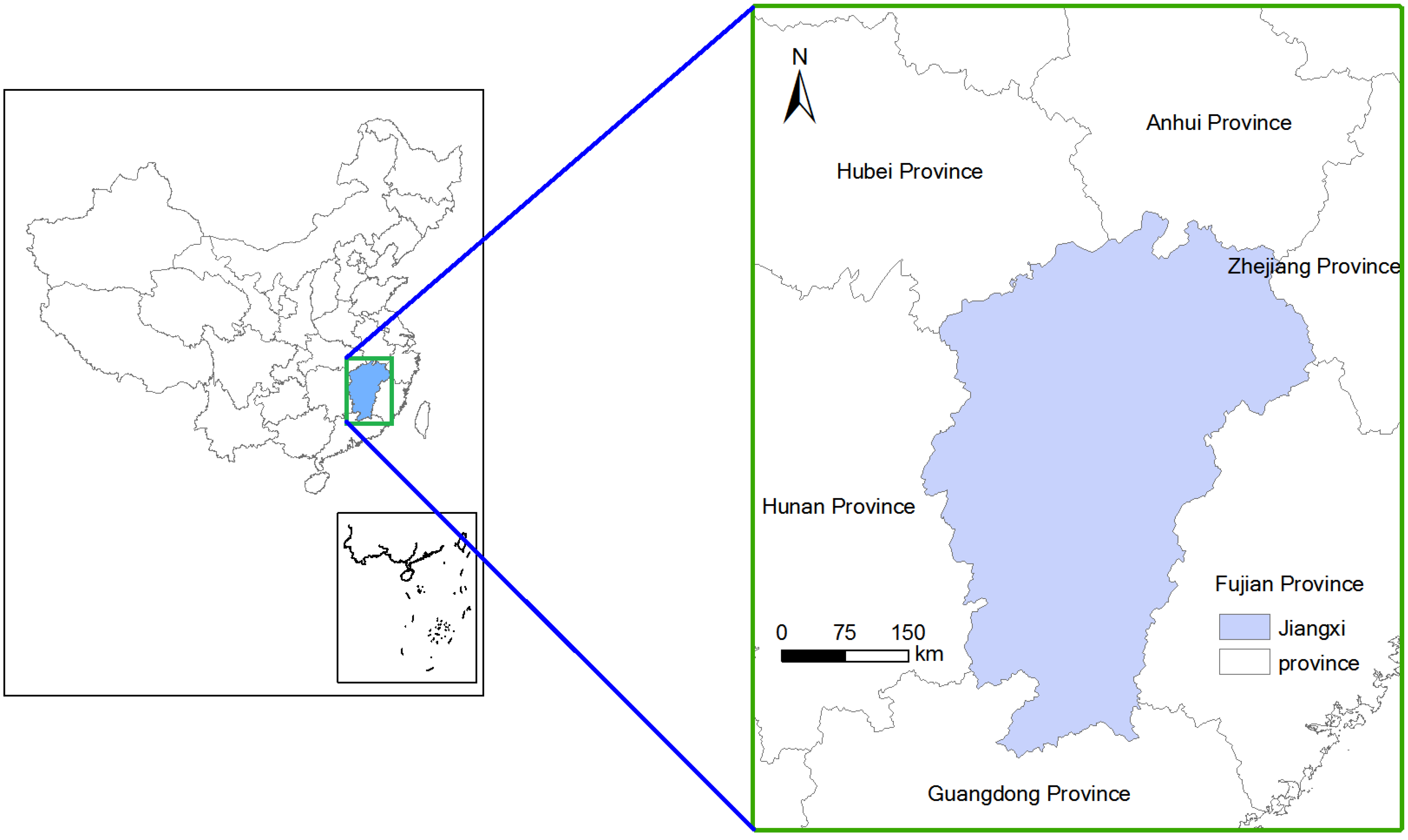
2.1. Study Area
2.2. Data
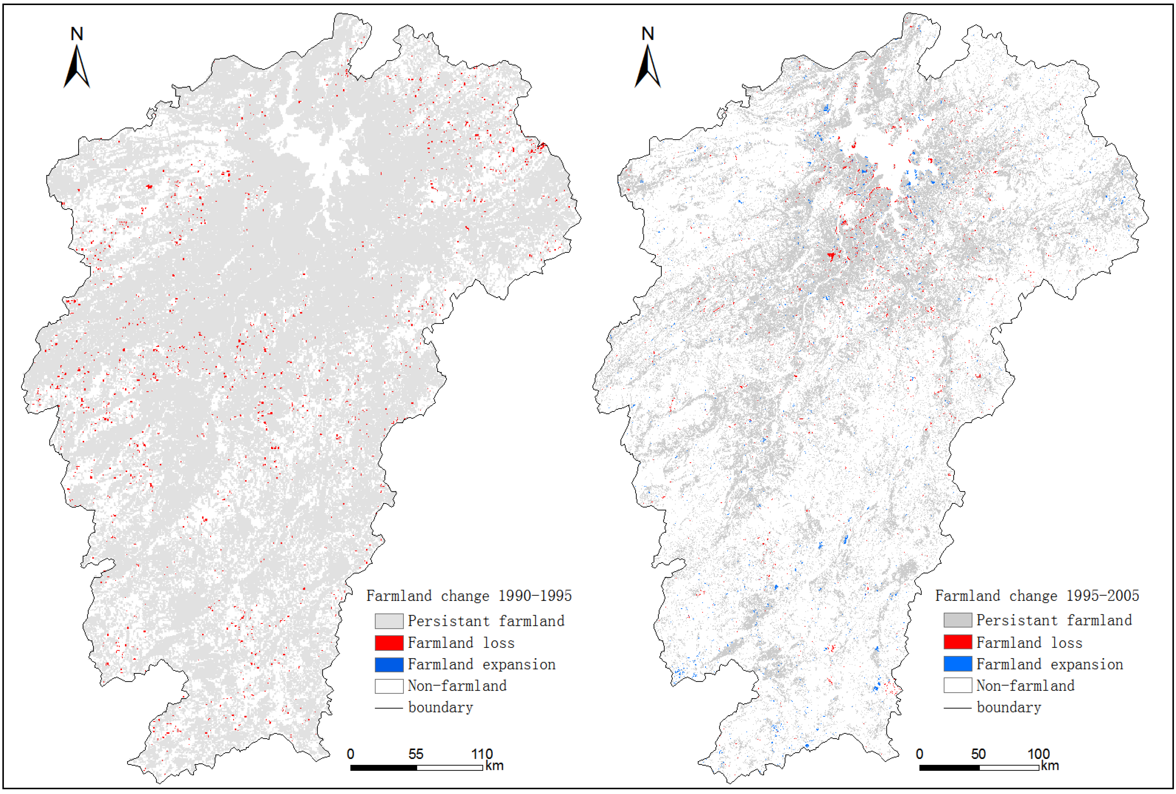
2.2.1. Land Use Data


| Land use/land cover class | Land use/land cover subclass |
|---|---|
| Farmland | Paddy field |
| Dry field | |
| Forest | Woodland |
| Shrubland | |
| Open woodland | |
| Grassland | High covered grass |
| Medium covered grass | |
| Low covered grass | |
| Water area | River and trench |
| Lake | |
| Reservoir | |
| Permanent glacier | |
| Beach | |
| Bottomland | |
| Built areas | City or town region |
| Village residential area | |
| Rest construct land | |
| Other covers | Sand land |
| Gobi | |
| Salted land | |
| Swamp | |
| Bare ground | |
| Bare rock | |
| Rest of used land |

2.2.2. Data of Biophysical Variables
2.2.3. Socio-Economical Data
2.3. Methods
2.3.1. Spatial Economical Model

| Variable Description | Spatial Resolution | Expected Sign * |
|---|---|---|
| Yield of agricultural product(y)-related variables | ||
| Cumulative temperature above 10 °C (day × °C) | 100 m | − |
| Annual precipitation (mm/year) | 100 m | − |
| Distance to forest edge (m) | 100 m | − |
| Soil depth (cm) | 100 m | − |
| Content of soil coarse sand (%) | 100 m | + |
| Slope (°) | 100 m | + |
| Elevation (m) | 100 m | + |
| Wage of agricultural labor(w)-related variables | ||
| Proportion of employees in the primary sector (%) | County | − |
| Rural labor force participation rate (%) | County | − |
| Rate of change of rural labor (%/year) | County | − |
| Rate of population urbanization (%) | County | + |
| Proportion of secondary sector’s output value (%) | County | + |
| GDP per capita (¥/capita) | County | + |
| Transportation cost(v)-related variables | ||
| Distance to central town(m) | 100 m | − |
| Distance to village (m) | 100 m | − |
| Distance to primary road (m) | 100 m | − |
| Structural characteristics in agriculture | ||
| Net income of farmer per capita (¥/capita) | County | ? |
| Average agricultural area per farmer (ha/farm) | County | + |
| Rate of change of farmer (%/year) | County | ? |
| Rate of change of employees in the primary sector (%/year) | County | ? |

2.3.2. Multivariate Logistic Regression Model


 is the natural logarithm of the maximum likelihood value. The range of − 2 is [0, +∞]. The smaller the AIC value is, the better the model will be fitted [50].
2.3.3. Sampling
3. Results


| Variables | Estimator (β) | Standard Error (SE) | Wald χ2 Statistics | p Value | EXP (β) |
|---|---|---|---|---|---|
| Wald-Chi-square: 523.987(p < 0.0001) | |||||
| Constant | 21.209 | 5.887 | 12.981 | 0.000 | 2 × 10⁹ |
| Cumulative temperature above 10 degrees | −0.001 | 0.000 | 12.439 | 0.000 *** | 0.999 |
| Annual precipitation | −0.009 | 0.004 | 5.852 | 0.016 * | 0.991 |
| Distance to forest edge | −0.001 | 0.000 | 9.273 | 0.002 ** | 0.999 |
| Soil depth | −0.005 | 0.011 | 0.191 | 0.662 | 0.995 |
| Content of soil coarse sand | 0.056 | 0.012 | 22.604 | 0.000 *** | 1.058 |
| Slope | 0.201 | 0.025 | 66.942 | 0.000 *** | 1.223 |
| Elevation | 0.003 | 0.001 | 8.126 | 0.004 ** | 1.003 |
| Proportion of employees in the primary sector | −0.013 | 0.007 | 3.203 | 0.074 | 0.987 |
| Rural labor force participation rate | −0.008 | 0.004 | 2.959 | 0.085 | 0.993 |
| Rate of change of rural labor | −0.090 | 0.048 | 3.611 | 0.050 * | 0.914 |
| Rate of urbanization | 0.058 | 0.009 | 41.730 | 0.000 *** | 1.060 |
| Distance to town | 7.0 × 10⁻⁵ | 0.000 | 17.243 | 0.000 *** | 1.000 |
| Distance to village | 8.0 × 10⁻⁵ | 0.000 | 1.476 | 0.224 | 1.000 |
| Distance to primary road | 2.0 × 10⁻⁵ | 0.000 | 1.256 | 0.262 | 1.000 |
| Net income of farmer per capita | −0.003 | 0.001 | 15.816 | 0.000 *** | 0.997 |
| Average agricultural area per farm | 2.404 | 1.203 | 3.993 | 0.046 * | 11.068 |
| Rate of change of employees in the primary sector | 0.059 | 0.042 | 1.931 | 0.165 | 1.060 |
| Variables | Estimator (β) | Standard Error (SE) | Waldχ2 Statistics | p Value | EXP (β) |
|---|---|---|---|---|---|
| Wald-Chi-square: 210.703 (p < 0.0001) | |||||
| Constant | 12.046 | 2.372 | 25.787 | 0.000 | 1.7× 10⁵ |
| Cumulative temperature above 10 degrees | −0.001 | 0.000 | 17.084 | 0.000 *** | 0.999 |
| Annual precipitation | −1.9 × 10⁻⁴ | 0.001 | 0.032 | 0.859 | 1.000 |
| Distance to forest edge | 2.6 × 10⁻⁴ | 0.000 | 6.556 | 0.010 ** | 1.000 |
| Soil depth | −0.051 | 0.011 | 23.670 | 0.000 *** | 0.950 |
| Content of soil coarse sand | −0.027 | 0.015 | 3.168 | 0.075 | 0.973 |
| Slope | 0.080 | 0.022 | 13.382 | 0.000 *** | 1.083 |
| Elevation | −0.001 | 0.001 | 1.184 | 0.277 | 0.999 |
| Proportion of employees in the primary sector | −0.015 | 0.006 | 5.736 | 0.017 * | 0.985 |
| Rural labor force participation rate | −0.014 | 0.005 | 8.751 | 0.003 ** | 0.986 |
| Rate of change of rural labor | −1.113 | 0.724 | 2.364 | 0.124 | 0.329 |
| Rate of urbanization | 0.031 | 0.011 | 7.639 | 0.006 ** | 1.032 |
| Proportion of secondary sector’s output value | 0.031 | 0.015 | 4.561 | 0.033 * | 1.032 |
| GDP per capita | 7.1 × 10⁻⁵ | 0.000 | 6.279 | 0.012 * | 1.000 |
| Distance to town | 4.4 × 10⁻⁵ | 0.000 | 11.315 | 0.001 ** | 1.000 |
| Distance to village | 3.5 × 10⁻⁵ | 0.000 | 26.371 | 0.000 *** | 1.000 |
| Distance to primary road | 1.5 × 10⁻⁵ | 0.000 | 1.102 | 0.294 | 1.000 |
| Net income of farmer per capita | −0.002 | 0.001 | 17.766 | 0.000 *** | 0.998 |
| Average agricultural area per farm | 2.851 | 0.909 | 9.835 | 0.002 ** | 17.297 |
| Rate of change of farm | 0.263 | 0.172 | 2.330 | 0.127 | 1.301 |
| Rate of change of employees in the primary sector | −2.380 | 0.618 | 14.838 | 0.000 *** | 0.093 |
| Model | AIC | PC | AUC | Kappa |
|---|---|---|---|---|
| First period model | 0.89 | 0.81 | 0.80 | 0.45 |
| Second period model | 1.22 | 0.70 | 0.70 | 0.41 |
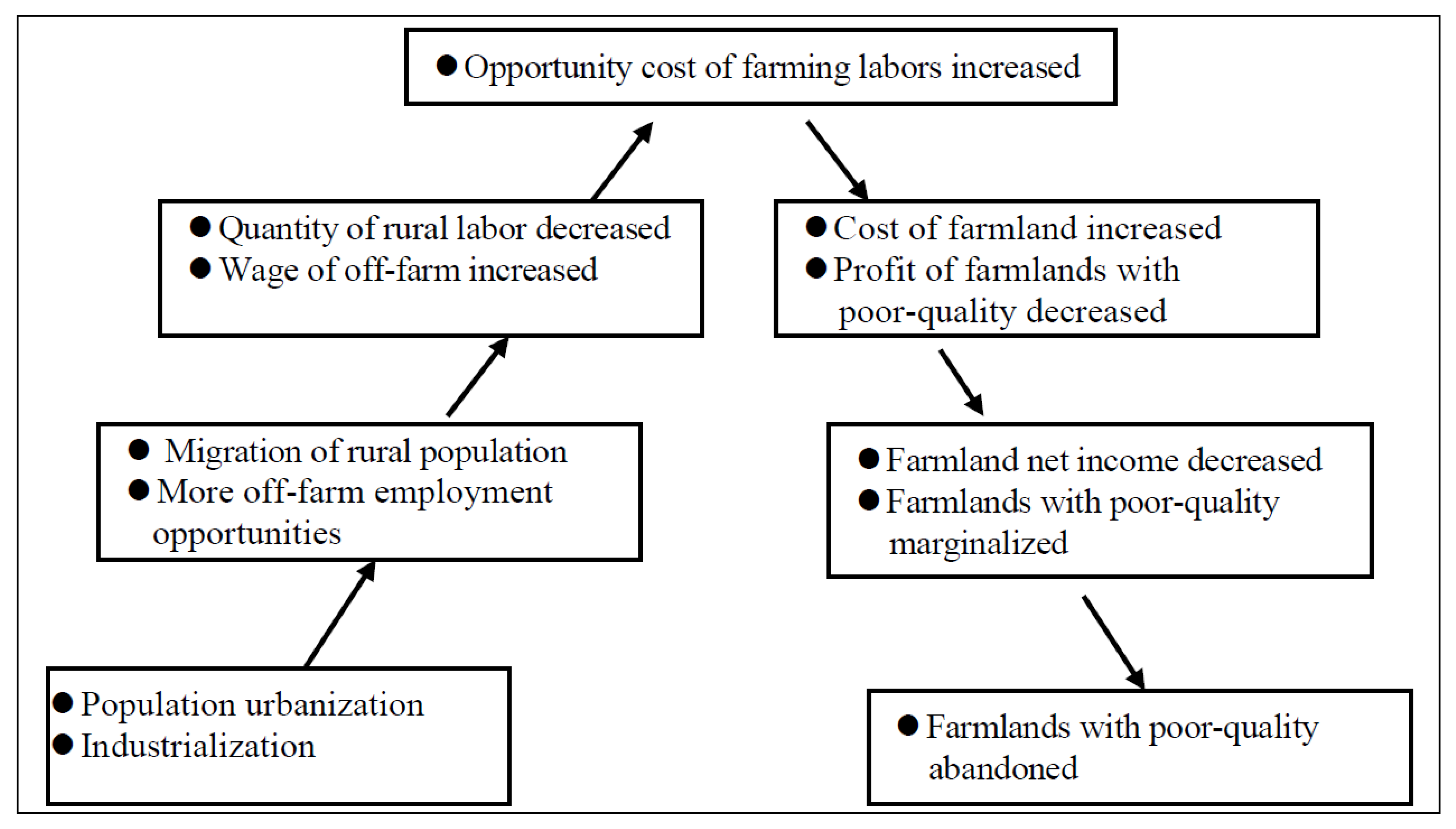
4. Discussion
5. Conclusions
Acknowledgements
Author Contributions
Conflicts of Interest
References
- Li, X. Core of global environmental change research: Frontier in land use and coverage change. Acta Geogr. Sin. 1996, 51, 553–558. [Google Scholar]
- Vitousek, P.M. Human domination of Earth’s ecosystems. Science 1997, 277, 494–499. [Google Scholar] [CrossRef]
- Xie, H.; Wang, P.; Huang, H. Ecological risk assessment of land use change in the Poyang Lake eco-economic zone, China. Int. J. Environ. Res. Public Health 2013, 10, 328–346. [Google Scholar] [CrossRef]
- Izquierdo, A.E.; Grau, H.R. Agriculture adjustment, land-use transition and protected areas in Northwestern Argentina. J. Environ. Manage. 2009, 90, 858–865. [Google Scholar] [CrossRef]
- Arnaez, J.; Lasanta, T.; Errea, M.P.; Ortigosa, L. Land abandonment, landscape evolution, and soil erosion in a Spanish mediterranean mountain region: the case of Camero Viejo. Land Degrad. Dev. 2011, 22, 537–550. [Google Scholar] [CrossRef]
- Nunes, A.N.; Coelho, C.O.A.; de Almeida, A.C.; Figueiredo, A. Soil erosion and hydrological response to land abandonment in a central inland area of Portugal. Land Degrad. Dev. 2010, 21, 260–273. [Google Scholar]
- Giupponi, C.; Ramanzin, M.; Sturaro, E.; Fuser, S. Climate and land use changes, biodiversity and agri-environmental measures in the Belluno province, Italy. Environ. Sci. Pol. 2006, 9, 163–173. [Google Scholar] [CrossRef]
- Hatna, E.; Bakker, M.M. Abandonment and expansion of arable land in Europe. Ecosystems 2011, 14, 720–731. [Google Scholar] [CrossRef]
- MacDonald, D.; Crabtree, J.R.; Wiesinger, G.; Dax, T.; Stamou, N.; Fleury, P.; Gutierrez Lazpita, J.; Gibon, A. Agricultural abandonment in mountain areas of Europe: Environmental consequences and policy response. J. Environ. Manage. 2000, 59, 47–69. [Google Scholar] [CrossRef]
- Li, X.; Zhao, Y. Forest transition, agricultural land marginalization and ecological restoration. China Popul. Res. Environ. 2011, 21, 91–95. [Google Scholar]
- Zhong, T.Y.; Huang, X.J.; Zhang, X.Y.; Wang, K. Temporal and spatial variability of agricultural land loss in relation to policy and accessibility in a low hilly region of southeast China. Land Use Pol. 2011, 28, 762–769. [Google Scholar] [CrossRef]
- Khanal, N.R.; Watanabe, T. Abandonment of land and its consequences. Mt. Res. Dev. 2006, 26, 32–40. [Google Scholar] [CrossRef]
- Weissteiner, C.J.; Boschetti, M.; Bottcher, K.; Carrara, P.; Bordogna, G.; Brivio, P.A. Spatial explicit assessment of rural land abandonment in the Mediterranean area. Glob. Planet. Change 2011, 79, 20–36. [Google Scholar] [CrossRef]
- Diaz, G.I.; Nahuelhual, L.; Echeverria, C.; Marin, S. Drivers of land abandonment in Southern Chile and implications for landscape planning. Landsc. Urban Plann. 2011, 99, 207–217. [Google Scholar] [CrossRef]
- Gibon, A.; Sheeren, D.; Monteil, C.; Ladet, S.; Balent, G. Modelling and simulating change in reforesting mountain landscapes using a social-ecological framework. Landsc. Ecol. 2010, 25, 267–285. [Google Scholar] [CrossRef] [Green Version]
- Houet, T.; Verburg, P.H.; Loveland, T.R. Monitoring and modelling landscape dynamics. Landsc. Ecol. 2010, 25, 163–167. [Google Scholar] [CrossRef] [Green Version]
- Mottet, A.; Ladet, S.; Coque, N.; Gibon, A. Agricultural land-use change and its drivers in mountain landscapes: A case study in the Pyrenees. Agric. Ecosyst. Environ. 2006, 114, 296–310. [Google Scholar] [CrossRef]
- Bakker, M.M.; Govers, G.; Kosmas, C.; Vanacker, V.; van Oost, K.; Rounsevell, M. Soil erosion as a driver of land-use change. Agric. Ecosyst. Environ. 2005, 105, 467–481. [Google Scholar] [CrossRef]
- Gisbert, J.M.; Ibanez, S.; Perez, M.A. Terrace abandonment in the Ceta Valley, Alicante Province, Spain. Adv. Geo. Ecol. 2005, 36, 329–337. [Google Scholar]
- Gellrich, M.; Baur, P.; Koch, B.; Zimmermann, N.E. Agricultural land abandonment and natural forest re-growth in the Swiss mountains: A spatially explicit economic analysis. Agric. Ecosyst. Environ. 2007, 118, 93–108. [Google Scholar] [CrossRef]
- Lakes, T.; Muller, D.; Kruger, C. Cropland change in southern Romania: A comparison of logistic regressions and artificial neural networks. Landsc. Ecol. 2009, 24, 1195–1206. [Google Scholar] [CrossRef]
- Nagendra, H.; Southworth, J.; Tucker, C. Accessibility as a determinant of landscape transformation in western Honduras: linking pattern and process. Landsc. Ecol. 2003, 18, 141–158. [Google Scholar] [CrossRef]
- Crk, T.; Uriarte, M.; Corsi, F.; Flynn, D. Forest recovery in a tropical landscape: What is the relative importance of biophysical, socioeconomic, and landscape variables? Landsc. Ecol. 2009, 24, 629–642. [Google Scholar] [CrossRef]
- Cocca, G.; Sturaro, E.; Gallo, L.; Ramanzin, M. Is the abandonment of traditional livestock farming systems the main driver of mountain landscape change in Alpine areas? Land Use Pol. 2012, 29, 878–886. [Google Scholar] [CrossRef]
- Figueiredo, J.; Pereira, H.M. Regime shifts in a socio-ecological model of farmland abandonment. Landsc. Ecol. 2011, 26, 737–749. [Google Scholar] [CrossRef]
- Corbelle-Rico, E.; Crecente-Maseda, R.; Sante-Riveira, I. Multi-scale assessment and spatial modelling of agricultural land abandonment in a European peripheral region: Galicia (Spain), 1956–2004. Land Use Pol. 2012, 29, 493–501. [Google Scholar] [CrossRef]
- Lambin, E.F.; Meyfroidt, P. Land use transitions: Socio-ecological feedback versus socio-economic change. Land Use Pol. 2010, 27, 108–118. [Google Scholar] [CrossRef]
- Lambin, E.F.; Turner, B.L.; Geist, H. Our Emerging understanding of the causes of land use and cover change. Glob. Environ. Change 2001, 11, 261–269. [Google Scholar] [CrossRef]
- Cao, G.Y.; Chen, G.; Pang, L.H.; Zheng, X.Y.; Nilsson, S. Urban growth in China: Past, prospect, and its impacts. Popul. Env. 2012, 33, 137–160. [Google Scholar] [CrossRef]
- Lu, Y.; Wang, F. From general discrimination to segmented inequality: Migration and inequality in urban China. Soc. Sci. Res. 2013, 42, 1443–1456. [Google Scholar] [CrossRef]
- Szabó, G.; Fehér, A. Marginalisation and multifunctional land use in Hungary. J. Agri. Sci. 2004, 15, 50–61. [Google Scholar]
- Van Doorn, A.M.; Bakker, M.M. The destination of arable land in a marginal agricultural landscape in South Portugal: An exploration of land use change determinants. Landsc. Ecol. 2007, 22, 1073–1087. [Google Scholar] [CrossRef]
- Xin, L.J.; Liu, X.B.; Tan, M.B. The rise of ordinary labor wage and its effect on agricultural land use in present China. Geogr. Res. 2011, 30, 1391–1400. [Google Scholar]
- Hao, H.G.; Li, X.B.; Zhang, J.P. Impacts of part-time farming on agricultural land use in ecologically-vulnerable areas in North China. J. Resour. Ecol. 2013, 4, 70–79. [Google Scholar] [CrossRef]
- Thematic Database for Human-earth System. Available online: http://www.data.ac.cn (accessed on 8 January 2013). (In Chinese)
- China Meteorological Data Sharing Service System. Available online: http://cdc.cma.gov.cn/home.do (accessed on 8 January 2013). (In Chinese)
- ArcGIS, Version 9.3; ESRI: Redlands, CA, USA, 2008.
- Statistic Bureau of Jiangxi. Available online: http://www.jxstj.gov.cn/Index.shtml (accessed on 8 Janurary 2013). (In Chinese)
- Li, X. Explanation of land use changes. Prog. Geogr. 2002, 21, 195–203. [Google Scholar]
- Angelsen, A. Forest Cover Change in Space and Time: Combining the Von Thünen and Forest Transition Theories; World Bank Publications: Washington, DC, USA, 2007; Volume 4117. [Google Scholar]
- Pereira, J.M.C.; Itami, R.M. GIS-based habitat modeling using logistic multiple-regression: A study of the MT Graham Red Squirrel. Photogramm. Eng. Remote Sens. 1991, 57, 1475–1486. [Google Scholar]
- Narumalani, S.; Jensen, J.R.; Althausen, J.D.; Burkhalter, S.; Mackey, H.E. Aquatic macrophyte modeling using GIS and logistic multiple regression. Photogramm. Eng. Remote Sens. 1997, 63, 41–49. [Google Scholar]
- Garcia, C.V.; Woodard, P.M.; Titus, S.J.; Adamowicz, W.L.; Lee, B.S. A logit model for predicting the daily occurrence of human caused forest-fires. Int. J. Wildland Fire 1995, 5, 101–111. [Google Scholar] [CrossRef]
- Xie, H. Analysis of regionally ecological land use and its influencing factors based on a logistic regression model in the Beijing-Tianjin-Hebei region, China. Resour. Sci. 2011, 33, 2063–2070. [Google Scholar]
- Wang, N.H.; Brown, D.G.; An, L.; Yang, S.; Ligmann-Zielinska, A. Comparative performance of logistic regression and survival analysis for detecting spatial predictors of land-use change. Int. J. Geogr. Inf. Sci. 2013, 27, 1960–1982. [Google Scholar] [CrossRef]
- Guneralp, B.; Reilly, M.K.; Seto, K.C. Capturing multiscalar feedbacks in urban land change: A coupled system dynamics spatial logistic approach. Environ. Plan. B-Plan. Des. 2012, 39, 858–879. [Google Scholar] [CrossRef]
- Lin, Y.P.; Chu, H.J.; Wu, C.F.; Verburg, P.H. Predictive ability of logistic regression, auto-logistic regression and neural network models in empirical land-use change modeling—A case study. Int. J. Geogr. Inf. Sci. 2011, 25, 65–87. [Google Scholar] [CrossRef]
- Gobin, A.; Campling, P.; Feyen, J. Logistic modelling to derive agricultural land use determinants: A case study from southeastern Nigeria. Agric. Ecosyst. Environ. 2002, 89, 213–228. [Google Scholar] [CrossRef]
- Feiberg, S. The Analysis of Crossclassfied Categorical Data, 2nd ed.; MIT Press: Cambridge, MA, USA, 1980. [Google Scholar]
- Hosmer, D.W.; Lemeshow, S. Applied Regression Analysis; Wiley: New York, NY, USA, 1989. [Google Scholar]
- SPSS, Version 21.0; SPSS China: Beijing, China, 2013.
- Wang, J.; Guo, Z. Logistic Regression Model—Methodology and Application; Higher Education Press: Beijing, China, 2001. [Google Scholar]
- Akaike, H. Information theory and an extension of the maximum likelihood principle. In Second International Symposium on Information Theory; Peterov, B.N., Caak, F., Eds.; Budapest: Akademiai Kiado, Hungary, 1973; pp. 267–281. [Google Scholar]
- Schneider, L.C.; Pontius, R.G. Modeling land-use change in the Ipswich watershed, Massachusetts, USA. Agric. Ecosyst. Environ. 2001, 85, 83–94. [Google Scholar] [CrossRef]
- Pijanowski, B.C.; Alexandridis, K.T.; Müller, D. Modelling urbanization patterns in two diverse regions of the world. J. Land Use Sci. 2006, 1, 83–108. [Google Scholar] [CrossRef]
- Maddala, G.S. Introduction to Econometrics; Macmillan: New York, NY, USA, 1988. [Google Scholar]
- Menard, S. Applied Logistic Regression Analysis; Sage: Thousand oaks, CA, USA, 1995; Volume 7. [Google Scholar]
- Cai, F.; Du, Y. Report on China’s Populaiton and Labor No.8 the Coming Lewisian Turing Point and Its Policy Implications; Social Science Academic Press: Beijing, China, 2007. [Google Scholar]
- Shi, T.C.; Li, X.B. Farmland abandonment in Europe and its enlightenment to China. Geogr. Geo. Inf. Sci. 2013, 29, 101–103. [Google Scholar]
- Stokstad, G. Exit from Farming and Land Abandonment in Northern Norway; Norwegian Forest and Landscape Institute: Oslo, Norway, 2010. [Google Scholar]
- Liu, C.W. Study on the Marginalizaiton of Arable Land in China; Science press: Beijing, China, 2009. [Google Scholar]
- Xin, L.J.; Fan, Y.Z.; Tan, M.H.; Jiang, L.G. Review of arable land-use problems in present-day China. Ambio 2009, 38, 112–115. [Google Scholar] [CrossRef]
© 2014 by the authors; licensee MDPI, Basel, Switzerland. This article is an open access article distributed under the terms and conditions of the Creative Commons Attribution license (http://creativecommons.org/licenses/by/3.0/).
Share and Cite
Xie, H.; Wang, P.; Yao, G. Exploring the Dynamic Mechanisms of Farmland Abandonment Based on a Spatially Explicit Economic Model for Environmental Sustainability: A Case Study in Jiangxi Province, China. Sustainability 2014, 6, 1260-1282. https://0-doi-org.brum.beds.ac.uk/10.3390/su6031260
Xie H, Wang P, Yao G. Exploring the Dynamic Mechanisms of Farmland Abandonment Based on a Spatially Explicit Economic Model for Environmental Sustainability: A Case Study in Jiangxi Province, China. Sustainability. 2014; 6(3):1260-1282. https://0-doi-org.brum.beds.ac.uk/10.3390/su6031260
Chicago/Turabian StyleXie, Hualin, Peng Wang, and Guanrong Yao. 2014. "Exploring the Dynamic Mechanisms of Farmland Abandonment Based on a Spatially Explicit Economic Model for Environmental Sustainability: A Case Study in Jiangxi Province, China" Sustainability 6, no. 3: 1260-1282. https://0-doi-org.brum.beds.ac.uk/10.3390/su6031260