Water Resource Vulnerability Characteristics by District’s Population Size in a Changing Climate Using Subjective and Objective Weights

Abstract

The goal of this study is to derive water resource vulnerability characteristics for South Korea according to individual district populations in a changing climate. The definition of water resource vulnerability in this study consists of potential flood damage and potential water scarcity. To quantify these vulnerabilities, key factors, or indicators affecting vulnerability, are integrated with a technique for order of preference by similarity to ideal solution (TOPSIS), which is a multi-criteria decision-making approach to determine the optimal alternative by considering both the best and worst solutions. The weight for each indicator is determined based on both the Delphi technique and Shannon’s entropy, which are employed to reduce the uncertainty in the process of determining the weights. The Delphi technique reflects expert opinions, and Shannon’s entropy reflects the uncertainty of the performance data. Under A1B climate change scenarios, medium-sized districts (200,000–300,000 inhabitants) are the most vulnerable regarding potential flood damage; the largest districts (exceeding 500,000 inhabitants) are found to be the most vulnerable with respect to potential water scarcity. This result indicates that the local governments of cities or districts with more than 200,000 inhabitants should implement better preventative measures for water resources. In addition, the Delphi and entropy methods show the same rankings for flood vulnerability; however, these approaches produce slightly different rankings regarding water scarcity vulnerability. Therefore, it is suggested that rankings from not only subjective but also objective weights should be considered in making a final decision to implement specific adaptive measures to climate change.

1. Introduction

Ensuring that cities have an adequate supply of water has become increasingly important as human populations continue to concentrate in urban areas. The global urban population has increased from 30% in 1950 to over 50% as of 2010 [1]. A similar trend has been recorded in South Korea, where more than 80% of the population now lives in urban areas. The rapidly growing demands of urban areas are straining local and regional water supplies, and concerns over urban water scarcity have become more prominent in this country.

Recent reports of water shortages have reflected deeper concerns about the impacts of climate change, population growth, and environmental regulations on water supplies [2]. Vörösmarty et al. [3] concluded that impending global-scale changes in population and economic development over the next 25 years will dictate the relationship between water supply and demand to a greater degree than will changes in the mean climate. Arnell [4] created an assessment of the ways in which water supply companies in England and Wales are adapting to climate change, evaluated in the context of a model describing the adaptation process. Medellín-Azuara et al. [5] employed downscaled hydrologic results from a dry-warm climate for the year 2085 in an economic-engineering optimization model of California’s statewide water supply system at 2050 water demand levels.

Flood damage issues are also a looming concern for urban areas. Due to the rapid increase in impervious area, the peak flow and time to achieve peak flow have become larger and shorter, respectively. Therefore, flood damage has grown unexpectedly concurrently with climate change. Extensive research on how climate change will affect flood vulnerability has been conducted in recent years to facilitate adaption to climate change. For example, Cameron et al. [6] explored the potential to assess the impacts of climate change on flood frequency for the gauged upland Wye catchment at Plynlimon, Wales, while accounting for uncertainty when modeling rainfall-runoff processes under current conditions. Prudhomme et al. [7] implemented appropriate methods that incorporate climate change uncertainty in flood risk assessment planning. Kay et al. [8] investigated the uncertainty in the impact of climate change on flood frequency in England through the use of continuous river flow simulations.

Extensive reports and research have demonstrated that the water scarcity phenomenon and flood damage issues are related to multiple considerations and constraints. Stewart [9] suggested that the goal of any multiple criteria decision making (MCDM) technique should be to provide help and guidance to a decision maker in discovering his or her most desired solution to a problem (or that course of action which best achieves the decision maker’s long-term goals). Therefore, vulnerability assessment is closely related to MCDM problems because it applies a spatial ranking to hazards [10,11,12]. For example, Li et al. [13] proposed a composite method based on variable fuzzy sets and the information diffusion method for disaster risk assessment. Jun et al. [12] developed a framework to quantify flood vulnerability in South Korea by considering climate change impacts, and Kim et al. [14] assessed the present and future vulnerability of water scarcity to climate change and variability in the South Korean provinces using a VIKOR (Visekriterijumska Optimizacija I Kompromisno Resenje) approach.

Unfortunately, only a few climate change vulnerability studies (e.g., [1,2]) have examined water resource vulnerability characteristics in relation to population size even though water resource vulnerability, including potential flood damage and potential water scarcity, is closely linked to not only climate change but also population growth. Therefore, this study developed vulnerability characteristics for flood and water scarcity for six different population size ranges in South Korea. The A1B climate change scenario of the Intergovernmental Panel on Climate Change (IPCC) was used, and the vulnerabilities were quantified using an MCDM method, which is a technique for order of preference by similarity to ideal solution (TOPSIS). In determining the weights for each criterion in the MCDM method, the uncertainty of the Delphi weights, acquired through a survey of experts, was reduced by comparing with the weights attained from Shannon’s entropy method.

2. Methods

2.1. Procedure

This study consisted of four steps to quantify the vulnerability of flood damage and water scarcity in districts within South Korea according to their population sizes (Figure 1). The first step was to classify the provinces according to their population sizes so that the vulnerability of flood damage and water scarcity could be assessed for each population group. The second step was to determine weighting values using Delphi survey and Shannon’s entropy, which provided subjective and objective weights, respectively. The third step was to identify the vulnerability using a TOPSIS method. The final step was to compare the vulnerability characteristics by population size. We focused on the vulnerability characteristics according to the population size of each district; therefore, vulnerability components and indicators from previous studies [14,15] were used in the current study.

Figure 1. Procedure used in this study.

Figure 1. Procedure used in this study.

2.2. Vulnerability Framework

The concept of vulnerability has a long history in the risk-hazard and social science literature [16], but it was introduced to the water sector only in 1992, after the Dublin conference declared freshwater to be a vulnerable resource. Vulnerability analysis is widely used in such disciplines as natural science, economy, poverty, climate change, water resources, human ecology, and geography. In recent years, interdisciplinary research teams have begun exploring the vulnerability of linked human environment systems [16].

A general conceptual model for vulnerability has emerged in the climate change literature that is similar to the wider use of the concept [17,18]. Adger [17] has summarized the vulnerability knowledge developed so far and reports considerable diversity in the concept and definition of vulnerability based on the discipline and context of each study. This study used a vulnerability framework that has been previously defined and applied by the IPCC report among the various frameworks. Vulnerability is defined as the degree to which a system is susceptible to, or unable to cope with, adverse effects of climate change, including climate variability and extremes. Vulnerability is also a function of the character, magnitude, and rate of climate variation to which a system is exposed, its sensitivity, and its adaptive capacity [19]. Although Hinkel [20] criticized the IPCC’s definition as being overly trendy and noted the resulting difficulty in making it operational, the definition is one of the most generic available and could therefore be considered a basis for further refinement. This situation has been the case in the global environmental change and sustainability science communities, who introduced the notion of a coupled social-ecological system in conceptualizing vulnerability [21,22]. Therefore, this study considered the IPCC vulnerability framework.

In the IPCC framework, climate exposure refers to a large variety of climate-related stimuli, such as a rise in sea level, temperature changes, precipitation changes, heat waves, heavy rainstorms, and droughts. Sensitivity is defined as the degree to which a system is affected, either adversely or beneficially, by climate-related stimuli. Adaptive capacity is the ability of a system to evolve to accommodate environmental hazards or policy changes and to expand the range of variability it can accommodate [17].

Although sensitivity, adaptive capacity, and vulnerability are useful integrative and multidimensional concepts for the evaluation of a water resources system’s status, they are also complex concepts that cannot be measured or observed directly. Thus, it has been necessary to identify proxy variables or indicators for use in assessment and modeling [23]. Desirable proxy indicators are variables that quantify, measure, and communicate relevant information, and they should simplify or summarize a number of important properties rather than focus on the isolated characteristics of a system. Indicators must be measurable or at least observable, and the methodology used to construct them should be transparent and understandable [24].

2.3. Weighting Values

This study used two different approaches to determine the weighting values. The Delphi technique was used to derive the subjective weights reflecting expert opinions. Shannon’s entropy was also used to derive the objective weights reflecting the uncertainty of the performance values.

2.3.1. Delphi Technique

The Delphi technique is a method for structuring a group communication process so that the process is effective in allowing a group of individuals, as a whole, to address a complex problem [25]. The Delphi technique is founded on a structured process for collecting and distilling knowledge from a group of experts through a series of questionnaires interspersed with controlled opinion feedback [26]. A chain of iterative questionnaires is sent to a group of purposely selected experts, who remain anonymous to one another [27]. The results of the previous questionnaires are returned to the respondents, who are then able to modify their responses. By the second of three rounds in this process, it is hoped that the experts will be able to arrive at a consensus on the estimation problem.

Rowe et al. [28] characterized the classical Delphi technique by four key features. (1) The Delphi participants are anonymous, which allows them to freely express their opinions without undue social pressure to conform from others in the group. Decisions are evaluated based on their merit rather than on who has proposed the idea. (2) Iteration allows the participants to refine their views in light of the group’s progress from round to round. (3) Controlled feedback informs the participants of the other participants’ perspectives and provides an opportunity for Delphi participants to clarify or change their views. (4) A statistical aggregation of the group’s responses allows for quantitative analysis and interpretation of the data.

2.3.2. Shannon’s Entropy

The entropy method developed by Shannon [29] provides objective weights with which to solve uncertainty information because it uses only the information from indicators. The influence of these indicators is obtained from the magnitude of their entropy weight. Smaller entropy values and larger entropy weights of certain index accounts in this index will provide more useful information to the decision maker [30].

For the MCDM problems, a performance matrix containing elements x_ij is constructed, where i represents the alternatives (i = 1, 2, …, m) and j represents the evaluating indicators (j = 1, 2, …, n). To apply the entropy method, a normalized decision matrix can be obtained as follows:

(1)

The uncertainty and entropy are smaller if a relatively large amount of information is available and vice versa [30]. As in Equation (4), the entropy is defined as

(2)

(3)

(4)

where n denotes the number of evaluated objects, and when f_ij = 0, f_ij = log f_ij = 0. Finally, the entropy weight of the ith evaluating indicator is determined as follows:

(5)

Where 0 ≤ w_i ≤ 1 and .

2.4. TOPSIS

The TOPSIS method was initiated for solving a multiple attribute decision-making problem with no articulation of preference information [31]. The TOPSIS technique is based on the concept that the ideal alternative solution has the best level outcome for all considered attributes, whereas the negative ideal solution is the one with the worst attribute values. A TOPSIS solution is defined as the alternative solution that is simultaneously farthest from the negative ideal solution and closest to the ideal alternative solution [32].

The TOPSIS procedure is presented in [33]. To apply the MCDM method, we respectively constructed an original indicator value matrix and a weight matrix:

X = (x_ij)_m×n

(6)

W = (w_i)_m

(7)

where i represents the alternatives, i.e., groups by population size (i = 1, 2, …, m, and j represents the evaluating indicators (j = 1, 2, …, n). The weighting values sum to 1, i.e., 0 ≤ w_i ≤ 1 and .

This step transforms various attribute dimensions into non-dimensional attributes, which allows for a direct comparison among the attributes. Therefore, the normalized performance matrix R is constructed by computing the normalized value r_ij as follows:

(8)

R = (r_ij)_m×n

(9)

where if i ∊ Θ₁ and if i ∊ Θ₂; moreover, Θ₁ is associated with the benefit attribute and Θ₂ is associated with the cost attribute.

By multiplying R by its associated weights W, the weighted performance matrix A is constructed:

A = w ⨂ R = (a_ij)_m×n

(10)

Moreover, the PIS (positive ideal solution) and the NIS (negative ideal solution) are respectively determined as follows:

(11)

(12)

The separation distances between each alternative and the PIS and between each alternative and the NIS are respectively defined to be

(13)

Therefore, the closeness coefficient for each alternative i can be defined as

(14)

(15)

Finally, all alternatives are ranked to determine the best alternative solution according to the closeness coefficient.

3. Materials

3.1. Study Area

South Korea covers an area of almost 100,000 km² and contains approximately 49 million people. South Korea consists of 16 provinces, including seven metropolitan cities (A01–A07) and 232 districts. The geographical and demographical characteristics of the provinces are presented in Figure 2a and Table 1, respectively.

3.2. Weighting Values on Each Criterion

The National Institute of Environmental Research (NIER) [15] performed a water resource vulnerability assessment that included water scarcity, flood control, and water quality for South Korea using the weighted sum method (WSM). We used the proxy variables and weighting values given by the NIER [15]. Moreover, 21 and 24 proxy variables and their weights were obtained from a survey of 11 experts, including hydrologists, water resources managers, and climate change experts, to assess flood vulnerability and water scarcity vulnerability, respectively [15].

Figure 2. Study area. Districts in South Korea according to their province and population. (a) Province classification; (b) Population classification.

Figure 2. Study area. Districts in South Korea according to their province and population. (a) Province classification; (b) Population classification.

Table 1. Characteristics of the 16 provinces in South Korea.

Provinces		Number of Districts	Area (km2)	Population (103 People)
Name	Symbol
Seoul	A01	25	605.3	10,039
Busan	A02	16	765.9	3446
Daegu	A03	8	885.6	2431
Incheon	A04	10	1029.4	2661
Gwangju	A05	5	501.3	1450
Daejeon	A06	5	539.9	1515
Ulsan	A07	5	1057.1	1094
Gyeonggi-do	A08	31	10,183.9	11,637
Gangwon-do	A09	18	16,874.9	1443
Chungcheongbuk-do	A10	12	7431.5	1479
Chungcheongnam-do	A11	16	8598.0	1959
Jeollabuk-do	A12	14	8051.0	1703
Jeollanam-do	A13	22	12,095.1	1740
Gyeongsangbuk-do	A14	23	19,026.1	2592
Gyeongsangnam-do	A15	20	10,531.1	3141
Jeju-do	A16	2	1845.9	547
Total		232	100,021.7	48,877

Table 1. Characteristics of the 16 provinces in South Korea.

Provinces		Number of Districts	Area (km2)	Population (103 People)
Name	Symbol
Seoul	A01	25	605.3	10,039
Busan	A02	16	765.9	3446
Daegu	A03	8	885.6	2431
Incheon	A04	10	1029.4	2661
Gwangju	A05	5	501.3	1450
Daejeon	A06	5	539.9	1515
Ulsan	A07	5	1057.1	1094
Gyeonggi-do	A08	31	10,183.9	11,637
Gangwon-do	A09	18	16,874.9	1443
Chungcheongbuk-do	A10	12	7431.5	1479
Chungcheongnam-do	A11	16	8598.0	1959
Jeollabuk-do	A12	14	8051.0	1703
Jeollanam-do	A13	22	12,095.1	1740
Gyeongsangbuk-do	A14	23	19,026.1	2592
Gyeongsangnam-do	A15	20	10,531.1	3141
Jeju-do	A16	2	1845.9	547
Total		232	100,021.7	48,877

The weights were determined through the use of two-round surveys, which were reduced to the variability of the weighting values determined by the expert groups. However, the weights obtained from the Delphi technique are subjective. Therefore, we also used Shannon’s entropy method to derive objective weights to effectively compare the influence of subjective and objective weights.

3.3. Performance Values

Datasets were obtained from a climate change adaptation tool based on GIS and created by the NIER [15] to create a performance matrix of South Korea’s 232 districts. The sensitivity and adaptive capacity data were acquired from Statistics Korea, the National Institute of Disaster Management Institute, and GIS analysis. The climate exposure data were acquired from the climate model and hydrologic model simulations under the A1B climate change scenario. These climate data were set by downscaling the outputs from the National Center for Atmospheric Research (NCAR) Community Climate System Model 3 with the PSU/NCAR Mesoscale Model (MM5) [34,35]. The outputs from the MM5 were used to derive hydrologic models of the land-surface process model and a hydrologic simulation program in FORTRAN, which in turn provided the hydrologic data.

4. Results

4.1. Population-Based Groups

We categorized the 232 districts into six groups (from G1 to G6) according to each district’s population size (Figure 2b and Table 2). The largest districts (populations exceeding 500,000) were classified as G1. The next-largest districts (populations exceeding 300,000) were placed in G2. Medium-sized districts, i.e., those with populations exceeding 200,000 and 100,000 were placed in G3 and G4, respectively. Small districts (fewer than 100,000 inhabitants) were grouped into G5 and G6. Seven metropolitan cities (A01–07) are contained within G1, G2 and G3. The other cities (A08–A16) are in the smaller districts.

Table 2. Grouping of districts according to population size.

Population Size	Symbol	Number of Districts
More than 500,000	G1	23
300,000–500,000	G2	42
200,000–300,000	G3	31
100,000–200,000	G4	39
50,000–100,000	G5	51
Less than 50,000	G6	46
Total		232

Table 2. Grouping of districts according to population size.

Population Size	Symbol	Number of Districts
More than 500,000	G1	23
300,000–500,000	G2	42
200,000–300,000	G3	31
100,000–200,000	G4	39
50,000–100,000	G5	51
Less than 50,000	G6	46
Total		232

4.2. Weights with Subjective and Objective Approaches

We used two different weights, as shown in Table 3 and Table 4. As noted above, “Delphi” corresponds to an average of expert opinions obtained from Delphi surveys. The weights for indicators (i.e., criteria) or for components (sensitivity, adaptive capacity, and climate exposure) based on the expert opinions gathered in the Delphi survey were quite different from those based on the data characteristics given by Shannon’s entropy, as expected. Considering the weights for different vulnerability components (sensitivity, adaptive capacity, and climate exposure), the entropy-based method led to relatively smaller weights for climate exposure according to both the flood and water scarcity vulnerabilities; however, the Delphi survey led to relatively larger weights. Nevertheless, the entropy-based weights for sensitivity were considerably higher than the Delphi-based weights for flood and water scarcity vulnerability. The opposite weights were derived with adaptive capacity, meaning that the entropy-based weights for flood damage and the Delphi-based weights for water scarcity were higher than the others.

Table 3. Weighting and indicator values for flood vulnerability.

Criteria	Weighting Value		Indicator Value
	Delphi	Entropy	Min.	Avg.	Max.
Sensitivity	0.27	0.42
Low-lying area of less than 10 m (km2)	0.10	0.067	0.0	17.5	266.2
Low-lying household of less than 10 m	0.10	0.061	0.0	2.5	61.9
Area ratio with banks (%)	0.07	0.153	0.0	2.6	21.1
Population density (persons/km2)	0.12	0.095	0.19	38.7	271.8
Total population (persons)	0.10	0.148	0.833	202.8	1040
Regional average slope (°)	0.11	0.190	0.8	11.5	23.0
Percentage of road area (%)	0.07	0.156	0.7	5.6	26.2
Cost of flood management over last three years (106 Korean won)	0.16	0.081	0.0	342.5	21129.5
Population affected by flood management over last three years (10 persons)	0.15	0.049	0.4	200.8	103.8
Adaptive Capacity	0.34	0.38
Financial independence (%)	0.13	0.192	7.4	28.0	90.5
Number of civil servants per population (persons/103 people)	0.07	0.208	25.0	55.0	90.8
GRDP (106 Korean won)	0.11	0.180	8.7	87.7	236.5
Number of civil servants related to water	0.13	0.104	0.0	0.4	7.9
Ratio of improved river section (%)	0.14	0.208	16.0	72.6	100.0
Capacity of drainage facilities (m3/min)	0.21	0.105	0.0	48.1	459.0
Flood controllability of reservoirs (106 m3)	0.21	0.003	0.0	11.3	616.0
Climate Exposure	0.39	0.19
Daily maximum precipitation (mm)	0.31	0.205	58.4	80.8	162.6
Days with over 80 mm of rainfall (days)	0.23	0.189	0.0	0.7	2.5
5-day maximum rainfall (mm/5 days)	0.19	0.205	92.6	141.6	273.1
Surface runoff (mm/day)	0.16	0.197	0.0	0.1	0.3
Summer precipitation (June–September) (mm)	0.11	0.205	311.8	605.1	933.9

Table 3. Weighting and indicator values for flood vulnerability.

Criteria	Weighting Value		Indicator Value
	Delphi	Entropy	Min.	Avg.	Max.
Sensitivity	0.27	0.42
Low-lying area of less than 10 m (km2)	0.10	0.067	0.0	17.5	266.2
Low-lying household of less than 10 m	0.10	0.061	0.0	2.5	61.9
Area ratio with banks (%)	0.07	0.153	0.0	2.6	21.1
Population density (persons/km2)	0.12	0.095	0.19	38.7	271.8
Total population (persons)	0.10	0.148	0.833	202.8	1040
Regional average slope (°)	0.11	0.190	0.8	11.5	23.0
Percentage of road area (%)	0.07	0.156	0.7	5.6	26.2
Cost of flood management over last three years (106 Korean won)	0.16	0.081	0.0	342.5	21129.5
Population affected by flood management over last three years (10 persons)	0.15	0.049	0.4	200.8	103.8
Adaptive Capacity	0.34	0.38
Financial independence (%)	0.13	0.192	7.4	28.0	90.5
Number of civil servants per population (persons/103 people)	0.07	0.208	25.0	55.0	90.8
GRDP (106 Korean won)	0.11	0.180	8.7	87.7	236.5
Number of civil servants related to water	0.13	0.104	0.0	0.4	7.9
Ratio of improved river section (%)	0.14	0.208	16.0	72.6	100.0
Capacity of drainage facilities (m3/min)	0.21	0.105	0.0	48.1	459.0
Flood controllability of reservoirs (106 m3)	0.21	0.003	0.0	11.3	616.0
Climate Exposure	0.39	0.19
Daily maximum precipitation (mm)	0.31	0.205	58.4	80.8	162.6
Days with over 80 mm of rainfall (days)	0.23	0.189	0.0	0.7	2.5
5-day maximum rainfall (mm/5 days)	0.19	0.205	92.6	141.6	273.1
Surface runoff (mm/day)	0.16	0.197	0.0	0.1	0.3
Summer precipitation (June–September) (mm)	0.11	0.205	311.8	605.1	933.9

In terms of sensitivity to flood damage, the expert groups placed more weight on the cost and population associated with past flood damage, but the data-driven weights were relatively low for those indicators. Additionally, a reservoir’s flood controllability (i.e., capacity) in terms of adaptive capacity for flood damage also differed between the Delphi and entropy approaches, meaning that reservoir capacity was critical for flood vulnerability but lacking in its assessment function. The indicators for water scarcity vulnerability, such as household water consumption and reservoir capacity, also presented discrepancies.

Table 4. Weighting and indicator values for water scarcity vulnerability.

Criteria	Weighting Value		Indicator Value
	Delphi	Entropy	Min.	Avg.	Max.
Sensitivity	0.31	0.38
Population density (persons/km2)	0.11	0.078	0.19	38.7	271.8
Total population (persons)	0.10	0.117	8.3	202.6	1040
Water supply (L/person/day)	0.07	0.143	299.7	359.5	444.1
Grain production per area (ton/km2)	0.07	0.092	0.0	29.5	300.1
Livestock production per area (km2)	0.06	0.101	0.6	65.4	630
Groundwater withdrawal (m3/year)	0.08	0.119	0.02	15.7	103.3
River water withdrawal (m3/year)	0.09	0.118	0.0	152.8	762.1
Household water consumption (103/m3/year)	0.15	0.051	0.2	11.5	143.2
Industrial water usage (103 m3/year)	0.14	0.077	0.0	13.2	279.7
Agriculture water usage (103 m3/year)	0.13	0.103	0.01	68.0	743.5
Adaptive Capacity	0.38	0.33
Financial independence (%)	0.12	0.152	7.4	27.9	90.5
Civil servants per population (persons/104 people)	0.05	0.159	25.0	55.0	90.8
GRDP (106 Korean won)	0.09	0.139	8.7	87.7	236.5
Number of civil servants related to water (persons)	0.09	0.085	0.0	0.4	7.9
Water supply distribution ratio (%)	0.15	0.165	74.5	89.6	100.0
Groundwater capacity (103 m3/year)	0.14	0.139	0.32	46.8	327.0
Reservoir for water supply capacity per area (103 m3)	0.21	0.093	0.0	1.3	22.3
Recycled water usage per area (103 ton/year)	0.15	0.068	0.18	14.9	210.0
Climate Exposure	0.31	0.29
Maximum number of continuous non-rainy days (days)	0.22	0.178	13.9	21.0	26.2
Winter (Dec, Jan and Feb; DJF) precipitation (mm)	0.18	0.173	0.5	1.1	3.4
Spring (Mar, Apr and May; MAM) precipitation (mm)	0.21	0.178	1.2	1.9	3.0
Winter (DJF) evapotranspiration (mm)	0.10	0.125	0.2	1.9	13.8
Spring (MAM) evapotranspiration (mm)	0.13	0.175	0.04	2.3	5.6
Underground outflow (mm)	0.15	0.171	0.0	0.3	0.7

Table 4. Weighting and indicator values for water scarcity vulnerability.

Criteria	Weighting Value		Indicator Value
	Delphi	Entropy	Min.	Avg.	Max.
Sensitivity	0.31	0.38
Population density (persons/km2)	0.11	0.078	0.19	38.7	271.8
Total population (persons)	0.10	0.117	8.3	202.6	1040
Water supply (L/person/day)	0.07	0.143	299.7	359.5	444.1
Grain production per area (ton/km2)	0.07	0.092	0.0	29.5	300.1
Livestock production per area (km2)	0.06	0.101	0.6	65.4	630
Groundwater withdrawal (m3/year)	0.08	0.119	0.02	15.7	103.3
River water withdrawal (m3/year)	0.09	0.118	0.0	152.8	762.1
Household water consumption (103/m3/year)	0.15	0.051	0.2	11.5	143.2
Industrial water usage (103 m3/year)	0.14	0.077	0.0	13.2	279.7
Agriculture water usage (103 m3/year)	0.13	0.103	0.01	68.0	743.5
Adaptive Capacity	0.38	0.33
Financial independence (%)	0.12	0.152	7.4	27.9	90.5
Civil servants per population (persons/104 people)	0.05	0.159	25.0	55.0	90.8
GRDP (106 Korean won)	0.09	0.139	8.7	87.7	236.5
Number of civil servants related to water (persons)	0.09	0.085	0.0	0.4	7.9
Water supply distribution ratio (%)	0.15	0.165	74.5	89.6	100.0
Groundwater capacity (103 m3/year)	0.14	0.139	0.32	46.8	327.0
Reservoir for water supply capacity per area (103 m3)	0.21	0.093	0.0	1.3	22.3
Recycled water usage per area (103 ton/year)	0.15	0.068	0.18	14.9	210.0
Climate Exposure	0.31	0.29
Maximum number of continuous non-rainy days (days)	0.22	0.178	13.9	21.0	26.2
Winter (Dec, Jan and Feb; DJF) precipitation (mm)	0.18	0.173	0.5	1.1	3.4
Spring (Mar, Apr and May; MAM) precipitation (mm)	0.21	0.178	1.2	1.9	3.0
Winter (DJF) evapotranspiration (mm)	0.10	0.125	0.2	1.9	13.8
Spring (MAM) evapotranspiration (mm)	0.13	0.175	0.04	2.3	5.6
Underground outflow (mm)	0.15	0.171	0.0	0.3	0.7

4.3. Vulnerability Rankings and Scores

We assessed flood and water scarcity vulnerability based on district size using two different weights, as shown in Equations (8)–(15). First, we normalized the performance values because they are mutually incompatible. Table 3 and Table 4 show that most of the measurement units are different; therefore, their magnitudes vary substantially. To make the various criterion scores compatible, they must be transformed into a common measurement unit while ensuring that the scores for each criterion range from 0 to 1. The normalization technique that uses the maximum or minimum values, i.e., Equation (9), is limited in considering large variations in the percentage or fractional ranges of the performance values. For example, performance values for the cost of flood management range from approximately 0 to 21.1 million Won; the ratios relative to the average range from approximately 0 to 62. Moreover, the performance values for the water supply range from approximately 330 to 444 L/person/day; the ratios relative to the average range from 0.83 to 1.2. Such smoothing effects of normalization can be overcome by other normalization techniques, such as the Z-score method, which, to some extent, uses the average and standard variation of the performance values. However, such a method is limited in that criteria with relatively large ranges of performance values might over-dominate the final scores.

In terms of flood vulnerability (Table 5 and Figure 2a and Figure 3a), G3 is the most vulnerable group, which is followed by G1. However, G4, G5, and G6 are relatively negatively vulnerable. Based on these findings, districts with 200,000–300,000 inhabitants are vulnerable to flood damage in a changing climate. Therefore, preventive measures for flood damage should be planned in these medium-sized districts. In terms of sensitivity rankings, G3 and G1 are highly vulnerable; G2 is the next most vulnerable group. The flood damage for these three regions may be adversely affected by climate-related stimuli. In terms of adaptive capacity, G1, G2, and G3 are the most vulnerable, i.e., they do not have the ability to evolve to accommodate environmental hazards or policy changes for increases in flood damage. In terms of climate exposure, G5 is the most vulnerable, while G6, G1, and G2 formed the second most vulnerable group; therefore, these groups have a high likelihood of exposure to extreme climate stimuli. Therefore, G1 is overly weak in terms of adaptive capacity, and districts belonging to G1 should plan to enhance their ability to accommodate environmental hazards.

In terms of water scarcity (Table 6 and Figure 2b and Figure 3b), G1 is the most vulnerable region, whereas G5 and G6 are relatively stable districts. Contrary to the results for flood vulnerability, districts with more than 500,000 inhabitants are vulnerable to water scarcity in a changing climate; therefore, preventive measures that ensure more stable water resources should be investigated. In terms of sensitivity and adaptive capacity, G1, G2 and G4 are highly vulnerable, whereas G3, G5, and G6 are relatively less vulnerable. Because G1, G2, and G4 have a high likelihood of extreme drought conditions, a numerical analysis of water scarcity should be conducted.

Table 5. Flood vulnerability according to the Delphi and entropy methods. Sensitivity, adaptive capacity, and climate exposure are normalized values.

Method	Symbol	Sensitivity	Adaptive Capacity	Climate Exposure	C*	Ranking
TOPSIS with Delphi	G1	0.510	0.656	0.370	0.363	2
	G2	0.474	0.565	0.411	0.306	3
	G3	0.546	0.498	0.412	0.871	1
	G4	0.460	0.487	0.413	0.263	4
	G5	0.354	0.412	0.419	0.163	5
	G6	0.193	0.311	0.394	0.023	6
TOPSIS with entropy	G1	0.515	0.715	0.465	0.398	2
	G2	0.490	0.555	0.498	0.331	3
	G3	0.513	0.494	0.489	0.886	1
	G4	0.427	0.521	0.488	0.266	4
	G5	0.297	0.471	0.477	0.138	5
	G6	0.165	0.403	0.474	0.004	6

Table 5. Flood vulnerability according to the Delphi and entropy methods. Sensitivity, adaptive capacity, and climate exposure are normalized values.

Method	Symbol	Sensitivity	Adaptive Capacity	Climate Exposure	C*	Ranking
TOPSIS with Delphi	G1	0.510	0.656	0.370	0.363	2
	G2	0.474	0.565	0.411	0.306	3
	G3	0.546	0.498	0.412	0.871	1
	G4	0.460	0.487	0.413	0.263	4
	G5	0.354	0.412	0.419	0.163	5
	G6	0.193	0.311	0.394	0.023	6
TOPSIS with entropy	G1	0.515	0.715	0.465	0.398	2
	G2	0.490	0.555	0.498	0.331	3
	G3	0.513	0.494	0.489	0.886	1
	G4	0.427	0.521	0.488	0.266	4
	G5	0.297	0.471	0.477	0.138	5
	G6	0.165	0.403	0.474	0.004	6

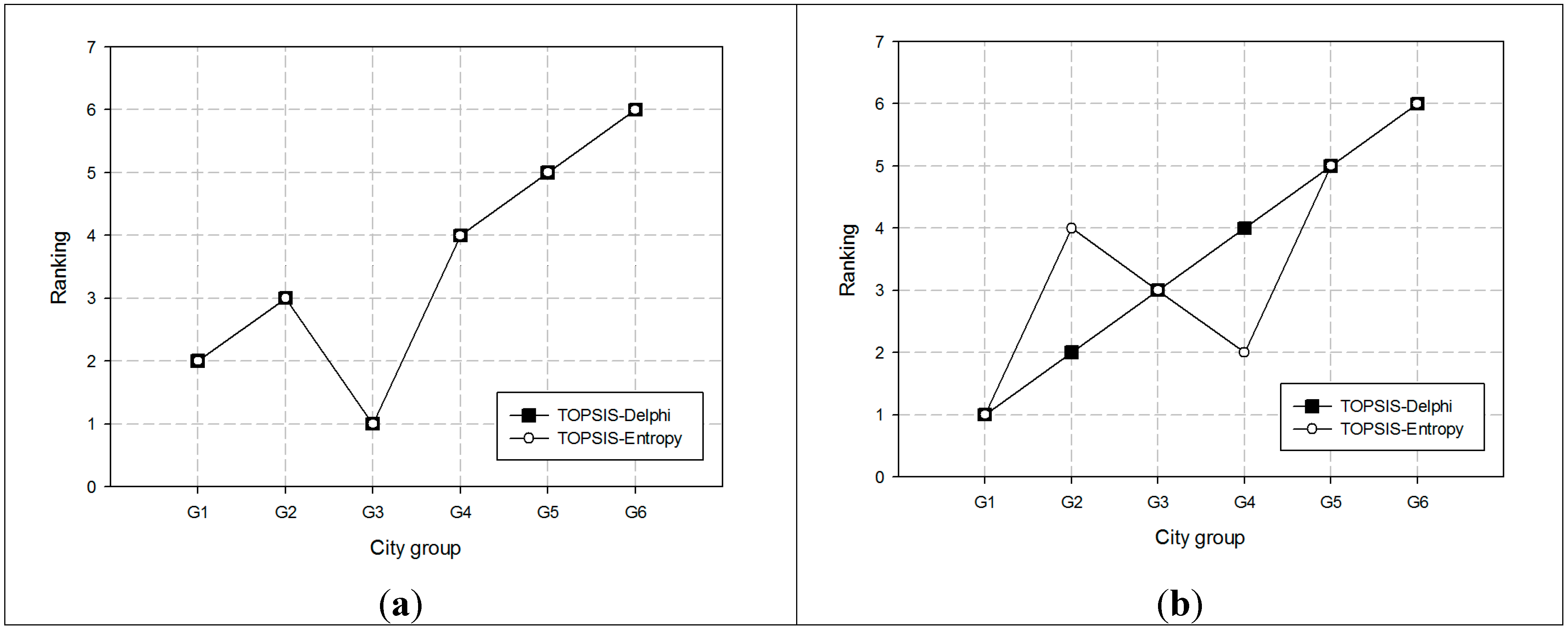
Figure 3. Rankings for flood and water scarcity vulnerability for each group based on the Delphi and Entropy methods. (a) Flood vulnerability; (b) Water scarcity vulnerability.

Figure 3. Rankings for flood and water scarcity vulnerability for each group based on the Delphi and Entropy methods. (a) Flood vulnerability; (b) Water scarcity vulnerability.

Table 6. Water scarcity vulnerability according to the Delphi and entropy methods. Sensitivity, adaptive capacity, and climate exposure are normalized values.

Method	Symbol	Sensitivity	Adaptive Capacity	Climate Exposure	C*	Ranking
TOPSIS with Delphi	G1	0.782	0.581	0.590	1.000	1
	G2	0.698	0.439	0.537	0.568	2
	G3	0.670	0.482	0.493	0.538	3
	G4	0.582	0.501	0.522	0.438	4
	G5	0.520	0.507	0.471	0.286	5
	G6	0.476	0.526	0.393	0.224	6
TOPSIS with entropy	G1	0.669	0.696	0.531	1.000	1
	G2	0.518	0.518	0.470	0.246	4
	G3	0.571	0.499	0.466	0.300	3
	G4	0.531	0.531	0.498	0.325	2
	G5	0.543	0.505	0.448	0.215	5
	G6	0.543	0.523	0.378	0.125	6

Table 6. Water scarcity vulnerability according to the Delphi and entropy methods. Sensitivity, adaptive capacity, and climate exposure are normalized values.

Method	Symbol	Sensitivity	Adaptive Capacity	Climate Exposure	C*	Ranking
TOPSIS with Delphi	G1	0.782	0.581	0.590	1.000	1
	G2	0.698	0.439	0.537	0.568	2
	G3	0.670	0.482	0.493	0.538	3
	G4	0.582	0.501	0.522	0.438	4
	G5	0.520	0.507	0.471	0.286	5
	G6	0.476	0.526	0.393	0.224	6
TOPSIS with entropy	G1	0.669	0.696	0.531	1.000	1
	G2	0.518	0.518	0.470	0.246	4
	G3	0.571	0.499	0.466	0.300	3
	G4	0.531	0.531	0.498	0.325	2
	G5	0.543	0.505	0.448	0.215	5
	G6	0.543	0.523	0.378	0.125	6

Furthermore, the two rankings determined using the Delphi and entropy methods are identical for flood vulnerability; however, these rankings are slightly different for water scarcity vulnerability (Figure 3). G2 is the second most vulnerable district according to the Delphi weights and the fourth most vulnerable based on the entropy method, while G4 is fourth and second, respectively. 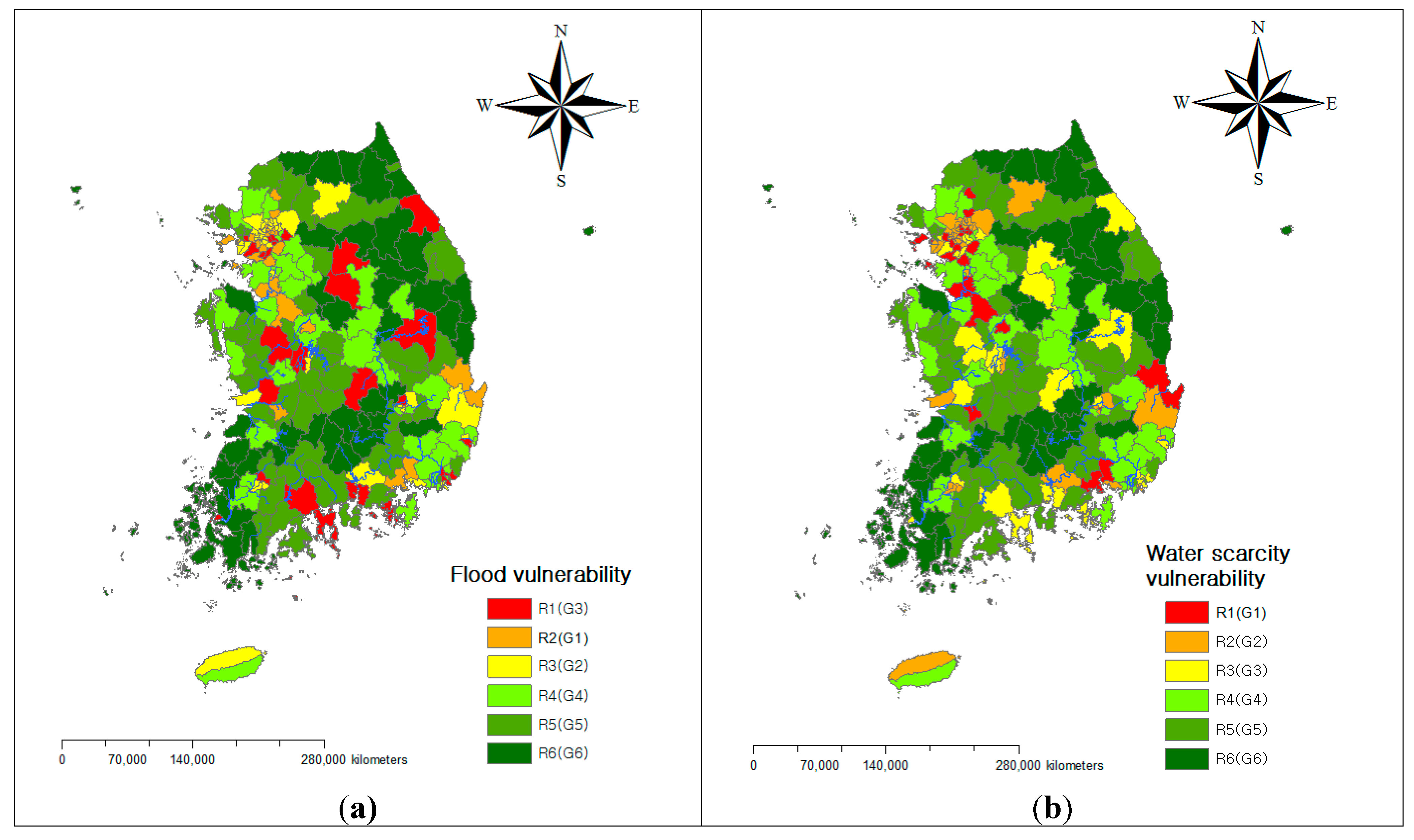Furthermore, Figure 4 presents the rankings based on the average vulnerability scores from the Delphi and entropy methods. Based on a comparison of the Delphi-based vulnerability and the entropy-based vulnerability, the results suggest that it is crucial to consider multiple possibilities for criteria weights to make robust decisions.

Figure 4. Distribution of flood and water scarcity vulnerability in districts based on the average vulnerability scores determined using the Delphi and entropy methods. (a) Flood vulnerability; (b) Water scarcity vulnerability.

Figure 4. Distribution of flood and water scarcity vulnerability in districts based on the average vulnerability scores determined using the Delphi and entropy methods. (a) Flood vulnerability; (b) Water scarcity vulnerability.

5. Conclusions

In this study, we derived flood and water scarcity vulnerabilities according to district population sizes under a specific climate change scenario, i.e., IPCC’s A1B. To quantify vulnerability, TOPSIS was used along with two approaches to determine the weights for key indicators of vulnerability. The weights based on Delphi surveys were complemented with the weights based on Shannon’s entropy.

The critical vulnerability characteristics according to population of individual districts were derived by applying the proposed procedure to vulnerability in South Korea. The medium-sized districts and the largest districts were the most vulnerable to flood damage and water scarcity. In particular, the results suggest that we could enhance factors related to water scarcity sensitivity and adaptive capacity for the largest districts. Additionally, the adaptive capacity of G1 to flood damage displays high vulnerability. In contrast, G5 and G6 (for flood damage and water scarcity) are negatively vulnerable. Therefore, districts with 50,000–100,000 or fewer than 50,000 inhabitants are relatively well-prepared and/or less vulnerable to climate change.

In the future, this study could be applied to develop particular preventive measures for various possible climate change scenarios with both subjective and objective weighting methods. In particular, large sets of scenarios and multiple MCDM approaches should be used to draw practical and robust adaptation strategies to climate change. Moreover, the multiple rankings could be integrated with aggregation methods (e.g., [32]).