1. Introduction
Nowadays, renewable energy resources such as solar, geothermal and wind, as well as heat losses from a wide range of industries, are increasingly being considered as energy sources that can help meet the world’s demand. Waste heat is often at relatively low temperatures, making it very difficult to convert such heat to electrical energy via conventional methods. As a result, many potential heat sources are wasted. Research on how to convert such heat resources to electricity is ongoing. Various cycles such as the organic Rankine, supercritical Rankine, Kalina, Goswami, and trilateral flash cycles have been investigated for electrical power production from low temperature heat resources [
1].
The operating principles for organic and steam-based Rankine cycles are similar. The main difference is the choice of working fluid. Refrigerants such as butane, pentane, hexane and silicon oil, which have lower boiling temperatures than water, can be used as working fluids in organic Rankine cycles (ORCs). These fluids are heated with low temperature heat like recovered waste heat and have properties that differ from those of water in many respects.
Organic Rankine cycles have been studied both theoretically [
2,
3] and experimentally [
4] since the 1970s, and exhibit efficiencies lower than 10% for small-scale systems. The first commercial organic Rankine cycles, which used geothermal and solar heat sources, appeared between 1970 and 1980. Numerous organic Rankine cycles have been installed in some countries (e.g., USA, Canada, Italy and Germany), although applications have also been reported in Finland, Belgium, Swaziland, Austria, Russia, Romania, India and Morocco.
There are numerous ORC equipment suppliers. Ormat and Turboden produce units for waste heat recovery for various industries (oil and gas, biomass, energy, packaging, cement and glass). The Swedish companies Upon AB and Entrans have installed several Organic Rankine cycles in Sweden in recent years. Upon AB has developed the Upon Power Box, a technology to generate electrical power from waste heat. Organic Rankine cycles with a total capacity of more than 1800 MWe are installed today around the world, most linked to biomass combined heat and power (CHP) and geothermal heat sources [
5].
The basic configuration and thermodynamic principles of steam and organic Rankine cycles are similar, but working fluids with thermodynamic properties that best suit the heat source are selected for organic Rankine cycles. Organic Rankine cycles have numerous advantages over conventional electrical generation systems:
Lower temperature applications
Low operation and maintenance costs
Compactness
No water consumption in some models
Smaller expanders with higher rotational speeds
Quiet operation
Simple start/stop procedures
Another advantage of organic working fluids is that the turbine in ORC requires a single-stage expander. This makes organic Rankine cycles simpler and more economic than typical Rankine cycles [
6]. Applications of ORCs include the following:
Biomass
Geothermal energy
Solar
Heat recovery
The saturation curve slope for organic working fluids can be positive (iso-pentane), negative (R22) or vertical (R11). These fluids are called “wet”, “dry” and “isentropic” fluids, respectively. Wet fluids (water) usually need to be superheated for electrical generation applications. Other organic fluids, of the dry or isentropic types, do not need to be superheated.
Much research has been carried out on organic Rankine cycles and their working fluids. Hung
et al. investigated efficiencies of ORCs using benzene, ammonia, R11, R12, R134a and R113 as working fluids. They concluded that isentropic fluids were the most suitable for recovering low-temperature waste heat [
7]. Angelino and Colonna developed a computer code with a commercial package for ORC analysis and optimization [
8]. Yamamoto
et al. investigated an ORC using HCFC-123 as a working fluid and conclude that this system has a better efficiency than one using water as a working fluid [
9]. Nguyen
et al. designed a Rankine cycle using n-pentane as the working fluid. This system produces 1.5 kW of electricity with a thermal efficiency of 4.3% [
10].
Wei
et al. reported a performance assessment and optimization of an ORC using HFC-245fa (3-pentafluoropropane) as a working fluid. The cycle was driven by exhaust heat. They concluded that usage of exhaust heat is a good way to improve system net power output and efficiency [
11]. Saleh
et al. investigated 31 pure components as working fluids for organic Rankine cycles. They concluded that ORCs typically operate between 100 and 30 °C for geothermal power plants at pressures mostly limited to 20 bar, but in some cases supercritical pressures are also considered. Thermal efficiencies are presented for various cycles. In the case of subcritical pressure processes, one has to identify (1) whether the shape of the saturated vapor line in the T-s diagram is bell-shaped or overhanging; and (2) whether the vapor entering the turbine is saturated or superheated. Moreover, for the case where the vapor leaving the turbine is superheated, an internal heat exchanger (IHE) may be used. The highest thermal efficiencies are obtained for high-temperature boiling substances with an overhanging saturated vapor line in subcritical processes within an IHE, e.g., for n-butane the thermal efficiency is 0.130. On the other hand, a pinch analysis of the heat transfer for the heat carrier with a maximum temperature of 120 °C to the working fluid shows that the largest amount of heat can be transferred to a supercritical fluid and the least to a high boiling temperature subcritical fluid [
12].
Mago and Chamra performed an exergy analysis of a combined engine-organic Rankine cycle, and conclude that the ORC with an engine improves the first and second law efficiencies [
13]. Mago
et al. analyzed regenerative organic Rankine cycles using dry organic working fluids; the cycles convert waste heat to electricity. The dry organic fluids considered are R113, R245ca, R123, and isobutane, which have boiling points ranging from −12 °C to 48 °C. The regenerative ORC was analyzed and compared with a basic ORC in order to determine the configuration that presents the best thermal efficiency and minimum irreversibility. The authors demonstrated that a regenerative ORC has a higher efficiency than the basic ORC, and also releases less waste heat when producing the same electricity with less irreversibility [
14].
Chacartegui
et al. investigated low temperature organic Rankine cycles as bottoming cycles in medium and large scale combined cycle power plants. The following organic working fluids were considered: R113, R245, isobutene, toluene, cyclohexane and isopentane. Competitive results were obtained for ORC combined cycles using toluene and cyclohexane as working fluids; as such, the systems exhibited reasonably high global efficiencies [
15].
Dai
et al. investigated ORCs for low-grade waste heat recovery with different working fluids. Thermodynamic properties for each working fluid were investigated and the cycles were optimized with exergy efficiency as an objective function using genetic algorithms. The authors showed that the cycles with organic working fluids were better than the cycle with water for converting low-grade waste heat to useful work. The cycle with R236EA exhibits the highest exergy efficiency. Adding an internal heat exchanger to the ORC did not improve the performance under the given waste heat conditions [
16].
Quoilin
et al. performed thermodynamic and economic optimizations of small-scale ORCs for waste-heat recovery applications, considering R245fa, R123, n-butane, n-pentane and R1234yf and Solkatherm as working fluids. They determined that the operating point for maximum power did not correspond to that of the minimum specific investment cost [
17].
Wang
et al. analyzed the performance of nine pure organic fluids at specific operating regions and foud that R11, R141b, R113 and R123 exhibited slightly better thermodynamic performances than the others, and that R245fa and R245ca were the most environmentally benign working fluids for engine waste heat-recovery applications [
18].
Qiu compared and optimized the eight most commonly applied working fluids and developed a performance ranking by means of the spinal point method [
19].
Hun Kang theoretically and experimentally investigated an ORC for generating electric power using a low-temperature heat source, using R245fa as a working fluid [
20].
Wang
et al. modeled a regenerative organic Rankine cycle for utilizing solar energy over a range of low temperatures, considering flat-plate solar collectors and thermal storage systems. They showed that system performance could be improved, under realistic constraints, by increasing turbine inlet pressure and temperature or lowering the turbine backpressure, and by using a higher turbine inlet temperature with a saturated vapor input. Compared to other working fluids, R245fa and R123 were identified as the most suitable for the system, in part due to their low operation pressures and the good performance they fostered [
21]. Quoilin
et al. described ORC applications, markets and costs, working fluid selection, and expansion machine issues [
22].
Clement
et al. presented an ORC system for recovering heat from a 100 kWe commercial gas turbine with an internal recuperator. They optimized the thermodynamic cycles, considering six working fluids, and analyzed several expanders to determine the most suitable [
23]. Branchini
et al. evaluated six thermodynamic indexes: cycle efficiency, specific work, recovery efficiency, turbine volumetric expansion ratio, ORC fluid-to-hot source mass flow ratio and heat exchanger size, for several cycle configurations: recuperation, superheated, supercritical, regenerative and combinations [
24]. Lecomptea
et al. developed a thermoeconomic design methodology for an ORC based on specific investment cost, operating conditions and part load behavior, which permitted selection of the optimum cycle [
25].
Zabek
et al. optimized a heat-to-power conversion process by maximizing the net power output. The process employed a trans-critical ORC with R134a as the working fluid. The authors developed a positive heat exchange/pressure correlation for the net power output with reasonable cycle efficiencies of around 10% for moderate device sizes, and concluded that, in order to design a comprehensive and dynamic unit configuration, a flexible cycle layout with an adjustable working fluid mass flow is required [
26]. Bracco
et al. experimentally tested and numerically modeled under transient conditions a small ORC, for which the main components are the R245fa working fluid, a plate condenser, an inverter-driven diaphragm pump, an electric boiler and a scroll expander. The latter is a hermetic device, derived from a commercial HVAC compressor, which generates about 1.5 kW of electrical power. Performance parameters for the overall cycle and its components were investigated and it was found that the lab management system software was able to simulate systems in transient conditions [
27]. Wang
et al. proposed an ideal ORC model to analyze the influence of working fluid properties on the thermal efficiency. The optimal operation conditions and the exergy destructions for various heat resource temperatures were also evaluated utilizing pinch and exergy analyses. The authors demonstrated that the Jacob number and the ratio of evaporating temperature and condensing temperature have significant influences on the thermal efficiency of an ORC and that a low Jacob number indicates attractive performance for a given operation condition [
28]. Yu
et al. simulated an actual organic Rankine cycle bottoming system using R245fa as a working fluid for a diesel engine, and conclude that approximately 75% and 9.5% of the waste heat from exhaust gas and from jacket water, respectively, can be recovered [
29]. Li
et al. experimentally analyzed the effect of varying working fluid mass flow rate and regenerator on the efficiency of a regenerative ORC operating on R123, and find that the power output is 6 kW and the regenerative ORC efficiency is 8.0%, which is 1.8% higher than that of the basic ORC [
30]. Maizza
et al. thermodynamically optimized ORCs for power generation and CHP considering various average heat source profiles (waste heat recovery, thermal oil for cogeneration and geothermal) They develop optimization methods for subcritical and trans-critical, regenerative and non-regenerative cycles, and present an optimization model to predict the best cycle performance (subcritical or trans-critical) in terms of exergy efficiency, considering various working fluids [
31]. Meinel
et al. presented Aspen Plus (V7.3) simulations of a two-stage organic Rankine cycle with internal heat recovery for four working fluids, in a two-part study. First, the exhaust gas outlet was constrained to 130 °C to stay above the acid dew point; Second, the pinch point of the exhaust gas heat exchanger was set to 10 K. For wet and isentropic fluids, the thermodynamic efficiencies of the two-stage cycle exceeded the corresponding values of reference processes by up to 2.2%, while the recuperator design benefited from using dry fluids compared to the two-stage concept [
32].
Mango
et al. presented a second-law analysis for the use of organic Rankine cycle (ORC) to convert waste energy to power from low-grade heat sources. The working fluids under investigation are R134a, R113, R245ca, R245fa, R123, isobutene, and propane, with boiling points between 243 and 48 °C. Some of the results demonstrated that ORC using R113 showed the maximum efficiency among the evaluated organic fluids for temperatures <380 K, and isobutene showed the best efficiency [
33].
Bu
et al. investigated system efficiency on six working fluids, R123, R134a, R245fa, R600a (isobutene), R600 (butane) and R290, in order to using geothermal energy as a heat source. The calculated results show that R290 and R134a, R600a (isobutene) is the more suitable working fluid for ORC in terms of expander size parameter, system efficiency and system pressure [
34].
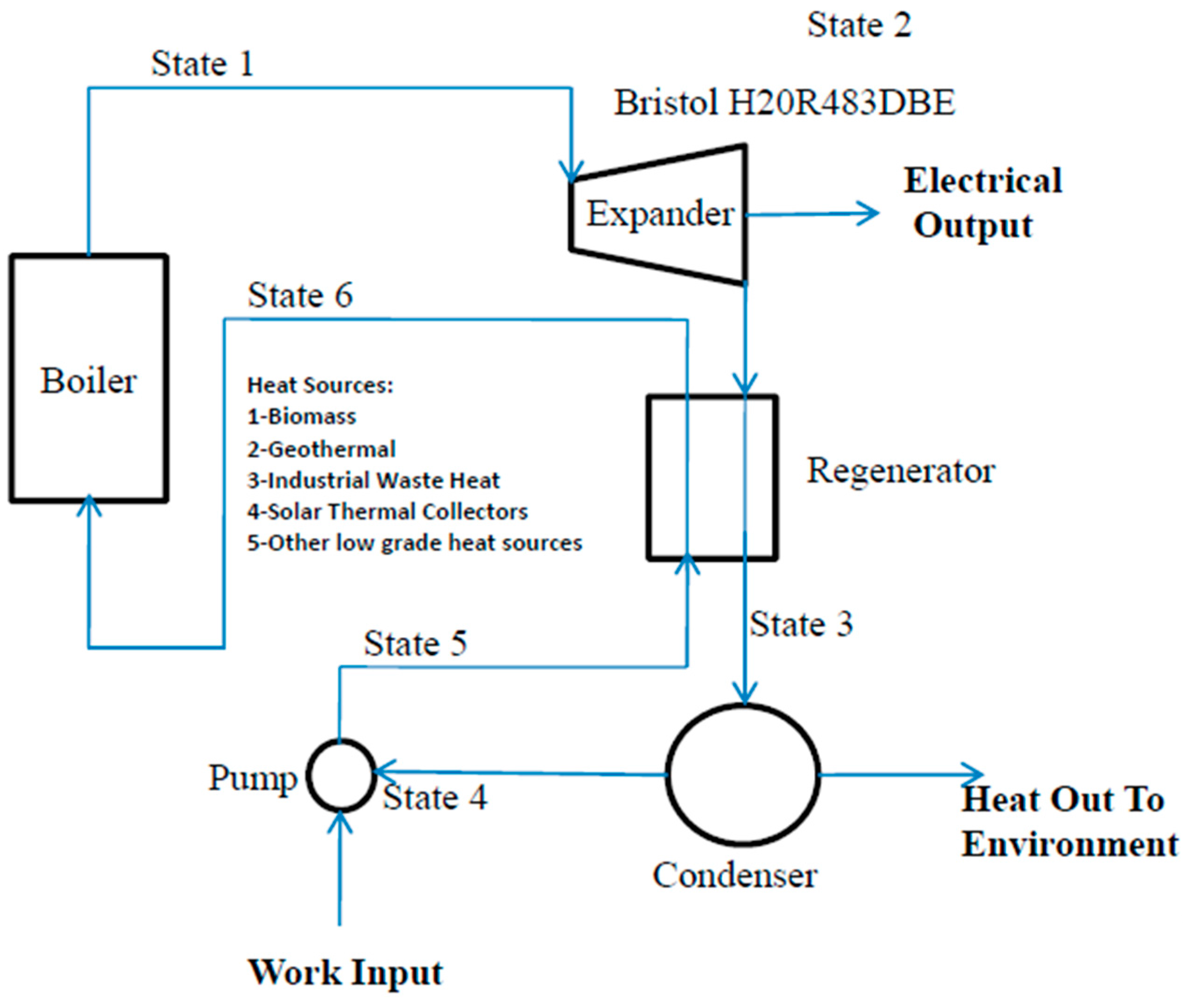
In the present study, the thermodynamic performance of regenerative organic Rankine cycles utilizing low temperature heat sources is simulated to assist in selecting proper organic working fluids. Bristol and thermodynamic models are used to investigate thermodynamic parameters such as output power and efficiency, and the cost rate of the product electricity is determined with exergo-economic analysis. Nine working fluids are considered in order to investigate which yields the greatest output power and exergy efficiency within system constraints. Exergy efficiency and cost rate of electricity are used as objective functions for the system optimization. Each of fluid is examined in order to achieve optimal operating conditions. The degree of superheat and pressure ratio are independent variables in the optimization.
4. Results and Discussion
For the system optimization, two independent parameters are selected as objective functions. In this case, the function to be optimized is exergy efficiency and the two indendent variables are pressure ratio (P
r) and degree of superheat (T
sh). The exergy efficiency function may not be related directly to pressure ratio and degree of superheat, but these two variables notably affect output power and the amount of required heat input. These two characteristics affect the exergy efficiency, since it is dependent both on electrical work output and heat input.
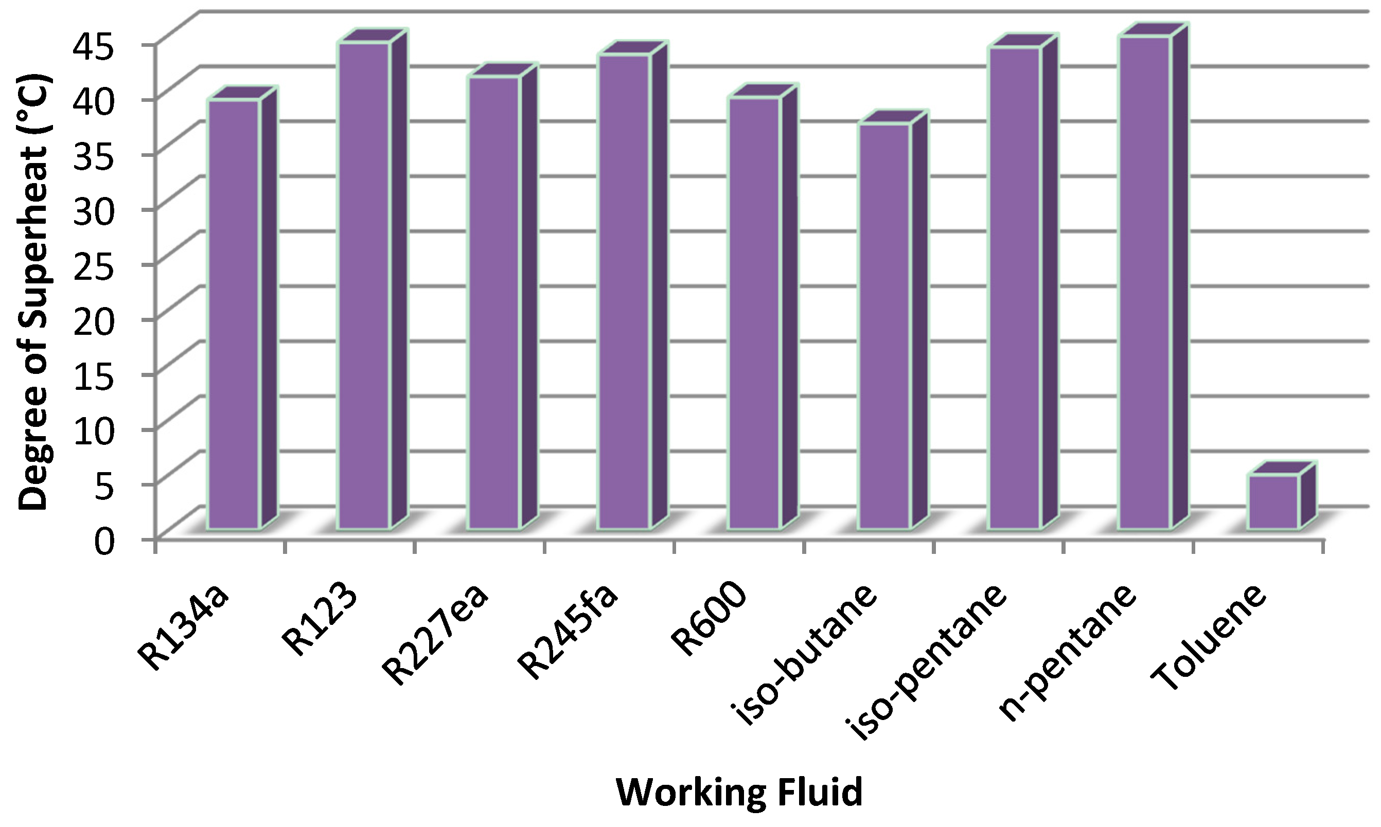
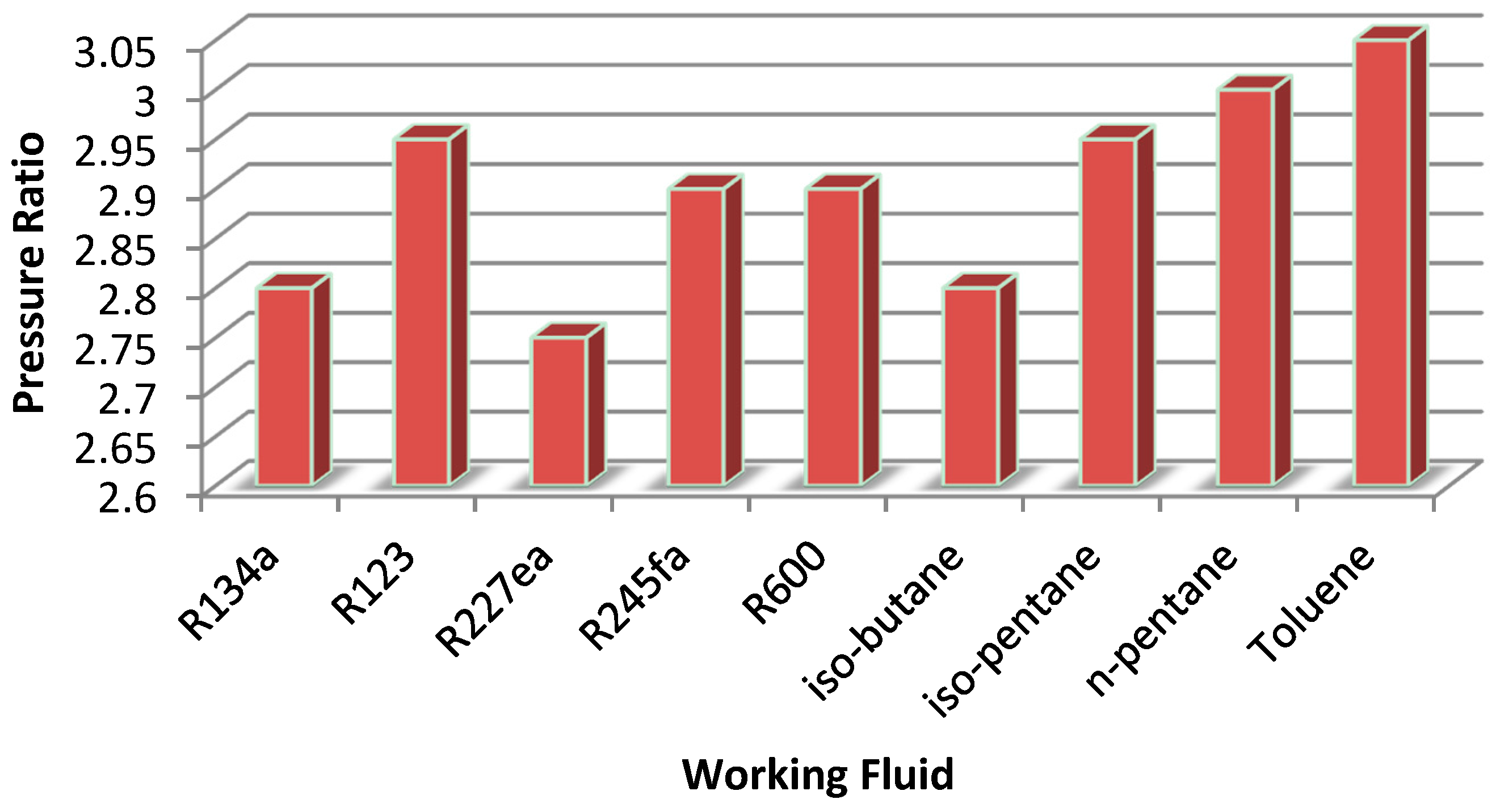
Figure 3 and
Figure 4 show the values of T
sh and P
r optimized for each of the working fluids. All of the dry fluids (e.g., R227ea, R134a, n-pentane, and R123) according to the specified constraints require a higher superheated temperature, which lies near the limit specified for the system. This limitation is due to the restrictions in condenser temperature, which taken to be 30 °C.
Figure 3.
Optimized values of degree of superheat for considered working fluids.
Figure 3.
Optimized values of degree of superheat for considered working fluids.
Figure 4.
Optimized values of pressure ratio for considered working fluids.
Figure 4.
Optimized values of pressure ratio for considered working fluids.
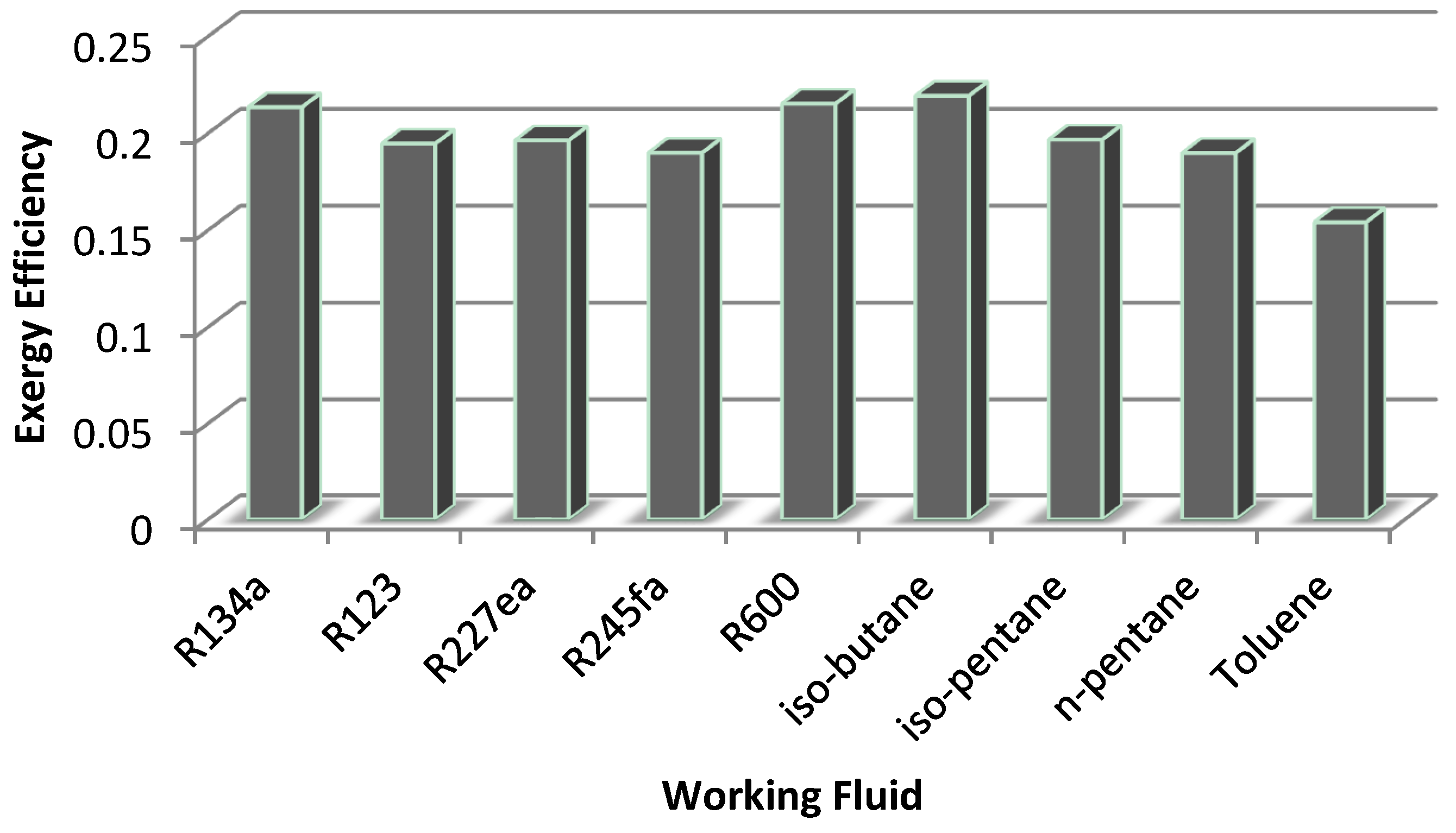
N-pentane exhibits the highest degree of superheat (44.9 °C) and Toluene the lowest (5 °C). The pressure ratio varies from 2.75 for R227ea to 3.3 for water. Increasing isentropic efficiency produces more output power, which increases system exergy efficiency. Depending on the working fluid, a higher degree of superheat may increase isentropic efficiency. When superheat is increased, the pressure ratio increases slightly for most fluids. The system exergy efficiencies for various working fluids are shown in
Figure 5, where values range from 15.4% for toluene to 21.9% for iso-butane. Systems using the working fluids iso-butane, R600 and R134a have the highest exergy efficiencies.
Figure 5.
System exergy efficiency for various working fluids.
Figure 5.
System exergy efficiency for various working fluids.
In
Table 5, the value of exergy efficiency, energy efficiency, isentropic efficiency, electricity cost rate, power output, expander rotational speed, pressure difference and system input heat are presented for the optimal condition.
Table 5.
Optimized thermodynamic parameter values for various working fluids.
Table 5.
Optimized thermodynamic parameter values for various working fluids.
| Fluid | % Exergy Efficiency | % Thermal Efficiency | % Isentropic Efficiency | (USD/kWh) | (kW) | Ω (RPM) | ΔP (kPa) | (kW) |
|---|
| R134a | 21 | 6.1 | 52 | 0.08 | 0.40 | 3917 | 1389.3 | 7.70 |
| R123 | 19 | 5.5 | 52 | 0.49 | 0.06 | 655 | 222 | 1.30 |
| R227ea | 20 | 5.6 | 51 | 0.15 | 0.20 | 3053 | 920.7 | 4.30 |
| R245fa | 19 | 5.4 | 52 | 0.29 | 0.10 | 684.9 | 366 | 2.28 |
| R600 | 22 | 6.1 | 51 | 0.14 | 0.23 | 1021 | 539 | 4.35 |
| Iso-butane | 22 | 6.2 | 52 | 0.10 | 0.30 | 1009 | 745.5 | 5.70 |
| Iso-pentane | 20 | 5.6 | 51 | 0.36 | 0.084 | 939 | 212.5 | 1.76 |
| n-pentane | 19 | 5.4 | 50 | 0.46 | 0.065 | 937 | 165.3 | 1.43 |
| Toluene | 15 | 4.4 | 50 | 1.43 | 0.021 | 836 | 58.3 | 0.56 |
Since exergy efficiency is a function of electrical work output and heat input, energy efficiency can be considered to be maximized when exergy efficiency is maximized, as they depend on the same variables. The lowest energy efficiency occurs for the working fluid toluene (4.4%) and the highest for iso-butane (6.2%). Systems using R600 and R134a exhibit relatively high energy efficiencies, both about 6.1%. The R600 and R134a fluids are appropriate for use in organic Rankine cycles as they provide the best efficiencies under the analyzed conditions.
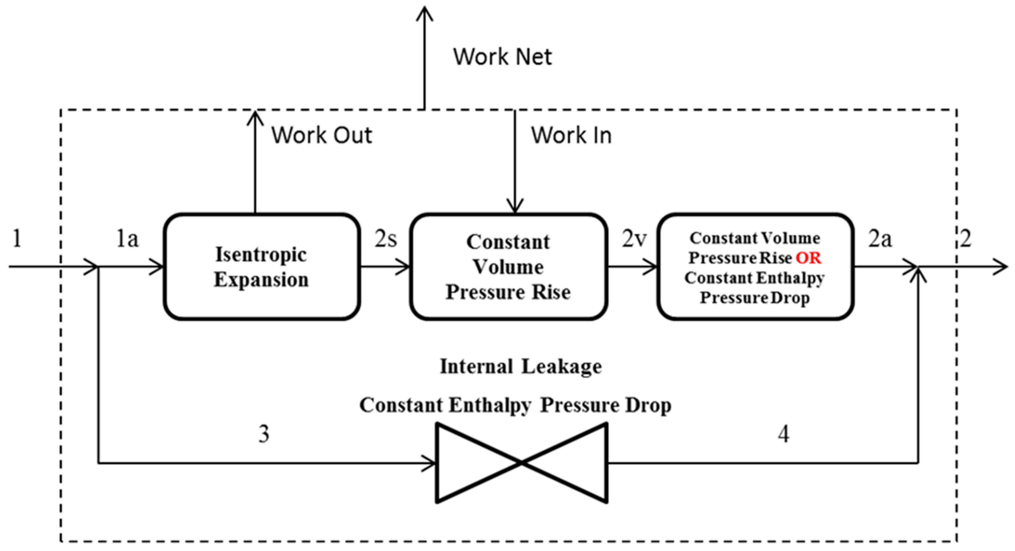
The isentropic efficiency of the expander is important in determining the amount of useful work it produces. Lower isentropic efficiencies mean that there are significant losses internally. As the fluid is expanded, the potential work instead is lost in overcoming friction and leakage losses. The isentropic efficiency for most working fluids considered is at or near the maximum value at the given conditions. The isentropic efficiency is considered tbe at a maximum if the pressure after the isochoric pressurization section is the same as the condenser pressure. If the pressures are higher or lower, throttling or additional work input are needed. These additional processes introduce irreversibilities since they do not contribute to useful work. High pressure ratios introduce additional leakage since the leakage mass flow rate is a function of input and output pressures. The system expander using R134a has the highest isentropic efficiency (52%) while that using n-pentane has the lowest (50.3%). These values are relatively low and suggest that this expander has significant losses due to friction and leakage.
From the exergo-economic analysis, the unit cost of electricity is calculated with the optimized results. The results are useful in identifying which fluid has the lowest electrical output unit cost. From
Table 5, toluene and R123 have unit electrical costs of 1.14 USD/kWh and 0.49 USD/kWh, respectively, which are the highest of all the working fluids considered. Systems using R134a, iso-butane and R600 exhibit the lowest unit costs of electricity, with values of 0.08, 0.10 and 0.14 USD/kWh, respectively. These costs reflect the lowest price that needs to be charged for the electricity and depend significantly on the amount of work output. The working fluids with the highest unit cost for electricity are seen to have the lowest electrical work outputs. Conversely, the working fluids with the highest electrical work outputs have the lowest electricity rates. For instance, systems using R134a, iso-butane and R600 generate 396.7, 301.7 and 226 W of electrical power, respectively, while those using toluene and R123 generate 20.8 and 61.3 W of electrical power, respectively.
The difference in pressure from inlet to outlet for the expander plays a large role in determining its work output. Since the torque produced by the expander is directly related to this pressure difference, it is useful to analyze this effect to help explain the work outputs of systems using each working fluid. The expander using R134a has the highest pressure difference (1389 kPa) and that using toluene the lowest (58.3 kPa). Other working fluids like R123 and n-pentane exhibit a low pressure difference, which corresponds to low electrical power outputs. The work output rate also corresponds to the heat input rate needed by the system. Systems using working fluids that lead to high work output rates such as R134a and iso-butane have high heat input rates. The system using R134a requires a heat input rate of almost 7.7 kW to produce 396.7 W of electrical power. The lowest heat input rate is needed for the system using toluene, which requires a heat input of 560 W to generate 20.8 W of electricity.
4.1. Exergy Analysis
Table 6 shows the exergy destruction breakdown for the system for each working fluid considered. The exergy destruction rate for the overall system using R134a is 1.3 kW. Most of the exergy destruction occurs is in the boiler (59.7%), and is due to the irreversible heat transfer processes in that component. The expander is responsible for almost 32% of the exergy destruction. These results suggest that there the improvement potentials are large for these components. This large share of exergy destruction in the expander is a consequence of the low expander isentropic efficiency of 52%. Large-scale systems typically have much higher expander isentropic efficiencies, approaching 80% to 90%. In order for the systems considered here to be competitive, the isentropic efficiency of its expander likely needs to improve. For the system using R227ea, the boiler is responsible for most of the system exergy destruction. Due to the larger amount of regeneration needed for this fluid (since it is a dry fluid), it exhibits relatively more exergy destruction in the regenerator. The condenser exergy destruction is also low for this system, and this can be attributed to the low temperature differences between the environment and the working fluid at the input state (see
Table 1). There are large improvement potentials for the boiler and the expander. The system using toluene has the lowest power production and has a large exergy destruction rate in the expander. The systems using iso-pentane and n-pentane have similar exergy destruction rates for the expander and the boiler. This is due to their similar chemical makeup of the working fluids. Note, however, that the exergy destroyed in the condenser is higher for the system using n pentane than the one using iso-pentane.
Table 6 shows the exergy destruction breakdowns for the systems using various working fluids. These results can help guide the selection of working fluid.
Table 6.
Working fluid exergy destruction percentage breakdown.
Table 6.
Working fluid exergy destruction percentage breakdown.
| Working Fluid | Exergy Destruction (% of Total in System) |
|---|
| | Boiler | Expander | Condenser | Pump | Regenerator |
|---|
| R134a | 59.67 | 32.18 | 0.3 | 0.61 | 7.25 |
| R123 | 65.44 | 25.76 | 0.35 | 0.08 | 8.37 |
| R227ea | 56.31 | 29.14 | 0.66 | 0.53 | 13.38 |
| R245fa | 64.53 | 25.99 | 0.09 | 0.13 | 9.25 |
| R600 | 59.77 | 30.79 | 0.28 | 0.24 | 8.92 |
| Iso-butane | 57.91 | 32.07 | 0.25 | 0.39 | 9.37 |
| Iso-pentane | 63.16 | 26.46 | 0.25 | 0.09 | 10.04 |
| n-pentane | 64.16 | 25.61 | 0.58 | 0.06 | 9.59 |
| Toluene | 44.54 | 49.85 | 1.05 | 0.04 | 4.52 |
4.2. Exergo-Economic Analysis
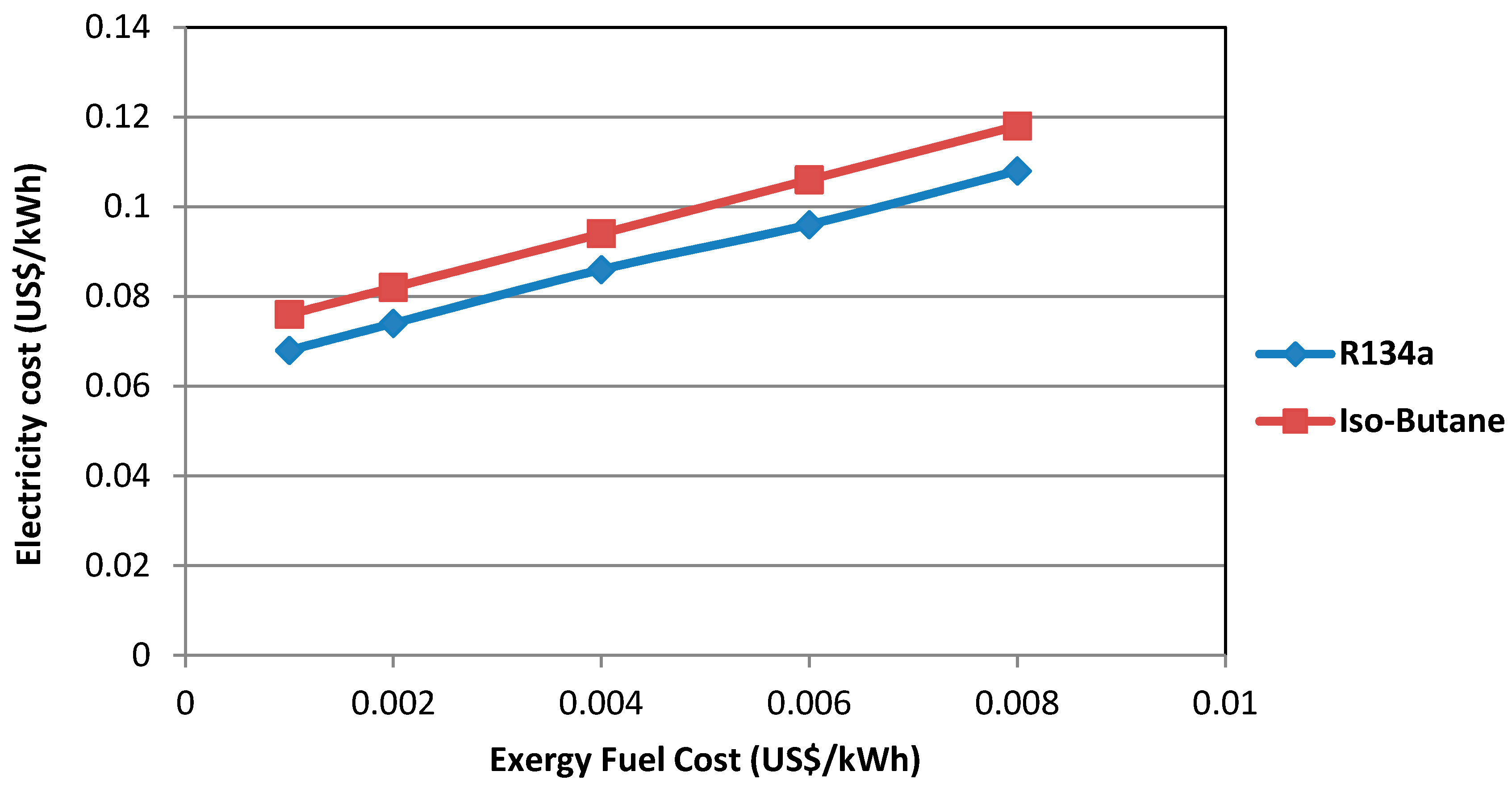
The exergo-economic cost balance equations are used in the analysis to determine the unit cost rate of electricity for an optimized exergy efficiency. The equation for exergy efficiency depends on the electrical power output and the heat input rate. The maximized value of exergy efficiency does not necessarily represent the maximum power output for the system at a particular pressure ratio. Optimizing the cost of electricity for systems using R134a and iso-butane is done by requiring EES to minimize the function for c
e (electricity unit cost rate), which is found in the cost rate balance for the expander. The same two independent variables, pressure ratio and superheat, are used. The bounds for the analysis do not change. Five unit exergy costs for input heat are considered: 0.001, 0.002, 0.004, 0.006 and 0.008 USD/kWh. These costs are used for comparison purposes to assess the sensitivity of the system to such changes. The same assumptions are used as outlined in the exergo-economic analysis section.
Figure 6 shows the minimized values for electricity rate for systems using R134a and iso-butane.
Figure 6.
Optimized values of electricity rate for systems using R134a and iso-butane working fluids.
Figure 6.
Optimized values of electricity rate for systems using R134a and iso-butane working fluids.
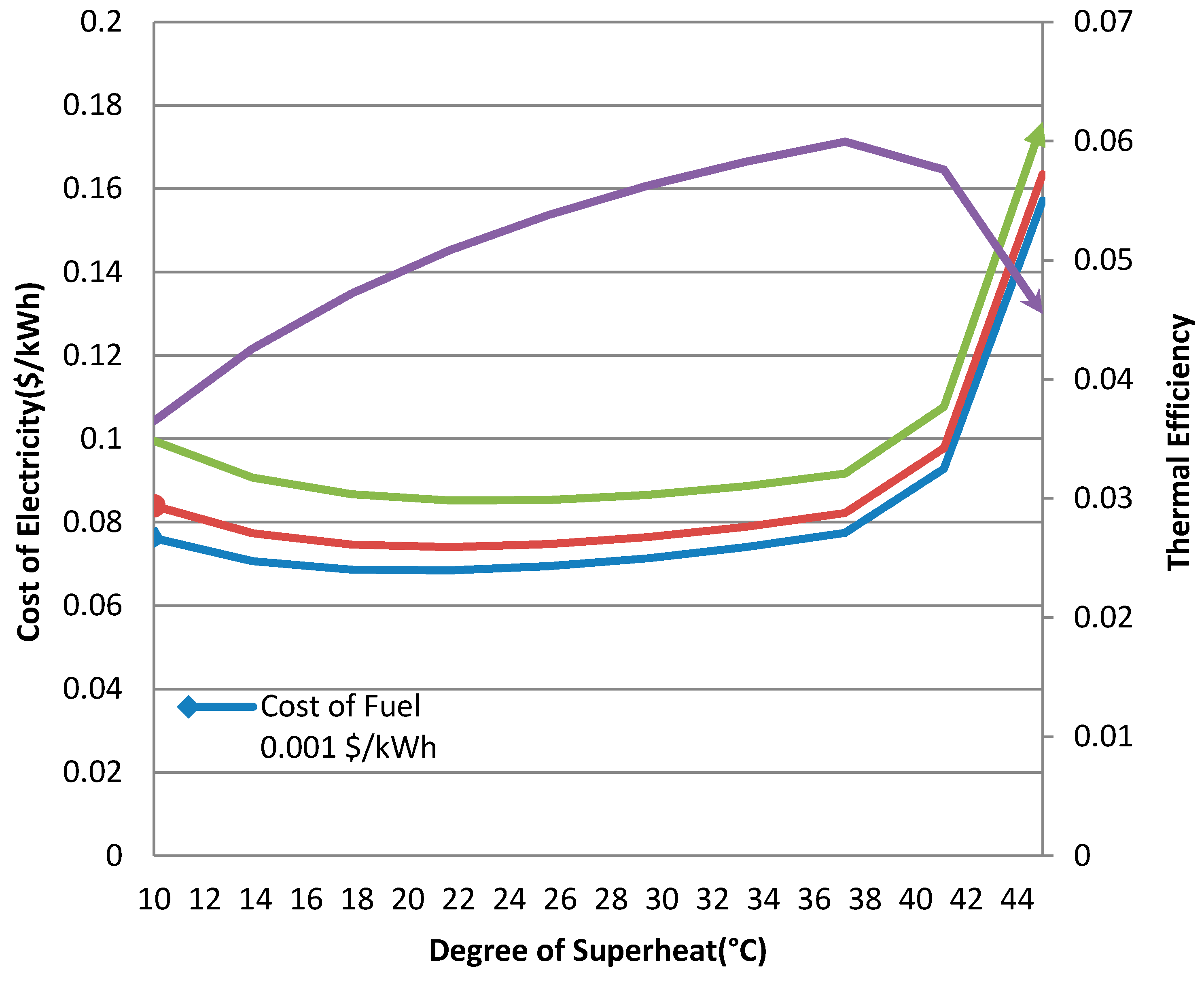
Thermal efficiency is dependent on two parameters including input heating energy and electricity output although the cost of electricity is dependent on the power output of the system so increase the cost of electricity is not necessarily reduced thermal efficiency.
Figure 7 shows the relationship between cost of electricity and thermal efficiency for R134a in the superheat temperature between 10 and 45 °C and the pressure ratio is 2.8.
Figure 7.
Electricity cost rate and thermal efficiency with varying superheat at optimal pressure ratio and three different fuel costs (R134a).
Figure 7.
Electricity cost rate and thermal efficiency with varying superheat at optimal pressure ratio and three different fuel costs (R134a).


