An Integrated Simulation Model for Dynamically Exploring the Optimal Solution to Mitigating Water Scarcity and Pollution

Abstract

An integrated optimization simulation model has been developed based on an input-output approach to mitigate water pollution and water scarcity through embedding environmental economic policies and applicable technologies into a complex environ-economic system to obtain an optimal set of policies and technologies that promotes the maximization of the regional economy under the constraints of water pollutant discharge and water availability. An empirical study is undertaken with the Source Region of Liao River as the target area to verify the performance of the model. The relationships between the water environment and socio-economic systems are presented by clarifying the trends in economic development, water pollutant discharge and water supply and demand during a time horizon from 2011 to 2020. The endogenously-formed optimal set of policies and industrial restructuring simultaneously facilitate the reduction of water pollutant discharge and water consumption and increase the water supply. The extent of the mitigation of water pollution and water scarcity via applied policies and technologies promoted by the subsidies provided by the government are specified, and the mechanism of the policy application and subsidization distribution is explained. This model has applicability for other regions in terms of giving an optimal solution via comprehensive assessment of all of the proposed sustainability-related policies with sufficient data accessibility to achieve regional sustainable development.

1. Introduction

Water, as a scarce input, is necessary for socio-economic activities conducted by humans. However, pressures on the water environment have escalated due to water resource overexploitation and water pollution, which have brought impacts to human health and sustainable socio-economic development [1,2]. This severe state makes it significant to clarify the relationships between the water environment and socioeconomic systems and to exploit eligible water environment management instruments for the prevention of water environmental degradation and the promotion of socioeconomic development compatible with the viability of the water environment. Thus, the solution for both water pollution control and the balance of the supply and demand of water resources necessitates full consideration of the social, economic and environmental settings.

Approaches and research on economic systems and the natural system have been applied to analyzing the relationship between the water environment and anthropogenic activities. Numerous studies have analyzed the water resource system [3,4,5] and water pollution [6] with a systematic dynamics modeling approach, which performs well for simulating scenarios of the water environment-economy interaction with a holistic consideration. Besides, a computable general equilibrium (CGE) model is another practical approach to capturing inter-linkages among industrial sectors, agents and markets, which has been intensively adopted to study the economic implications of water environmental policies [7,8,9].

The input-output (IO) model, as one innovative approach to detecting the interrelations and interdependencies among production sectors, has been extended and linked with resource utilization and pollutant emission to illustrate the interrelations between economy, environment and resources [10,11,12]. Environmental IO models have been widely applied to study atmospheric pollution and energy consumption. The levels of atmospheric pollutant emission, the environmental repercussions of a variety of patterns of the final demand and abatement costs have been addressed [13,14]. In addition, energy sources and air pollutants have been analyzed simultaneously from the perspective of energy balance and mass balance [15,16]. Specifically, studies of model construction to optimize biomass-related activities aided by IO analysis for regional bioenergy promotion have been carried out [17].

With regard to water resources, IO models have been adopted to study the induced effects on water resources resulting from socioeconomic activities, especially in countries and regions confronted with water scarcity challenges [18,19]. Some contributions have investigated sectoral water consumption based on an extended IO model to investigate the largest water consumer, which provides the possibility of designing economic and environmental policies oriented towards water saving [20,21]. Besides, water footprint analysis and virtual water trade analysis based on modified IO models have become popular instruments to evaluate direct and indirect freshwater use from the production and consumption perspectives, as well as water embedded in products, used in the whole production chain and traded between regions or exported to other countries [22,23,24,25].

The water pollution extended IO model has been used to investigate the relationship between water pollution and the economy [26,27,28,29] and for focusing on how pollution responds to changes in pollution coefficients and final demand to obtain shadow prices for different pollutants [30]. However, only a few studies have taken water pollution and water demand into consideration simultaneously within the framework of the IO model. The structure of water demand and water pollution has been evaluated by creating an emission inventory based on the IO table for Chongqing [31]. An integrated hydro-economic accounting framework has been constructed following the tradition of the economic-ecological IO model to track water consumption and water pollution, leaving the economic system and water flows in the hydrological system [32].

However, most of these studies are focused on investigating and clarifying inter-relationships between the water environment system and demographic, economic and lifestyle conditions with static IO analysis. Few studies have referred to embedding applicable technologies and associated environmental economic policies for environmental impact mitigation into complex socioeconomic systems and solving a dynamic optimization problem based on integrated modeling with the IO approach.

In order to obtain an optimal solution with a holistic consideration, we explore an integrated optimization simulation model (IOSM) based on an extended IO model. The IOSM is expected to clarify the interrelations between the water environment system and socioeconomic systems, to identify an optimal set of technologies and policies that is most effective and to realize total control of water pollutant discharge and the balance of the water supply and water demand with the least economic sacrifice. The extent to which the proposed policies and technologies will have influence on the mitigation of water pollution and water scarcity will be simulated for the period 2011 to 2020. The variation of renewable energy production and greenhouse gas (GHG) emissions induced by policy application and constraints for the water environment will also be analyzed. The optimization will be solved via the application of LINGO programming, a non-linear optimization software package released by LINDO Systems Incorporated.

2. Methodology

In this study, an extended IO table will be newly compiled with water as the primary input involved in the production of goods and services and water pollutants and GHG emission generated by production activities and household consumption as environmental indicators. The linearity of the relationships between sector output and the amount of water consumption, water pollutant discharge and GHG emission is presumed in order to combine the water environment and socioeconomic activities [33]. The proposed policies for water pollution control and the promotion of the water supply and demand balance are expected to form an optimal combination through a comparison of scenarios according to specific conditions.

2.1. Outline of the Model

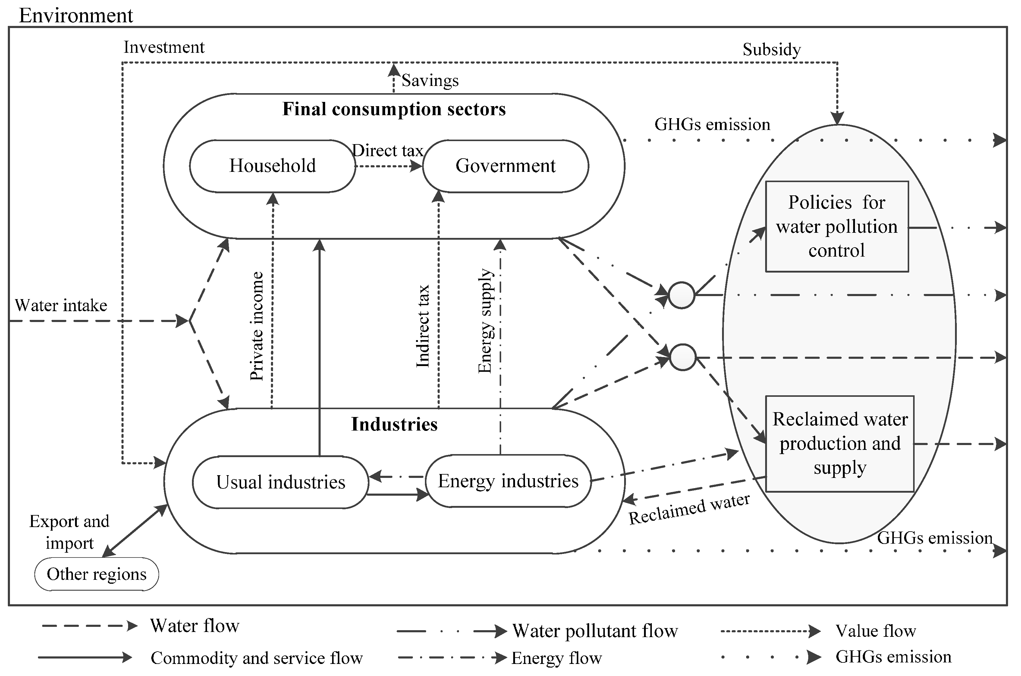
The model framework contains three major economic entities, including usual industries, energy industries and final demand sectors, and the proposed polices and technologies, which are integrated into a holistic environmental-socioeconomic system through the embedded material flow, value flow and energy flow. As shown in Figure 1, four subsystems within the whole system were determined. The socio-economic subsystem is elaborated as the production activities of industrial sectors, private and government consumption, investment and stock changes and net exports. Subsidies for the promotion of policy application are sourced from government savings. Reclaimed water, defined as the end product of waste water reclamation that meets the water quality for biodegradable materials, suspended matter and pathogens, is introduced into the water resource subsystem, which depicts the balance of the water demand and supply [34]. The water pollution control subsystem is utilized to calculate the amount of water pollutants generated from the production and consumption activities and that are discharged into water bodies (rivers, lakes, etc.) after introducing pollution abatement technologies. The energy and GHG emission subsystem additionally involves the production of renewable energy. It also clarifies the variation in GHG emissions resulting from the constraints of water pollutant discharge and water availability.

Figure 1. Outline of the integrated optimization simulation model.

Figure 1. Outline of the integrated optimization simulation model.

2.2. Mathematic Form of the Model

2.2.1. Water Supply and Demand Balance

The water supply is set to be no less than the water demand. The water supply contains freshwater and the newly-introduced reclaimed water (ReWS; endogenous; en). The freshwater supplied by surface water and groundwater is set to be no larger than the available freshwater supply (AFWS; exogenous; ex), which is determined by the water supply ability of surface water projects and groundwater projects collectively. The water demand for human activities is determined by population size, demographic structure and level of economic development and variation in the industrial structure.

$${\displaystyle \sum _{\text{m}}{Ci}^m\cdot X^m}(t)+{\displaystyle \sum _r{Ch}^r\cdot Z^r(t)}<=SWS(t)+GWS(t)+ReWS(t)$$

(1)

$$SWS(t)+GWS(t)<=AFWS(t)$$

(2)

where $X^m$ and $Z^r$ are the production of industry m and the population of lifestyle r, respectively (en); ${Ci}^m$ and ${Ch}^r$ are the freshwater consumption coefficients of industry m and lifestyle r (ex); SWS and GWS are the surface water supply and groundwater supply (en); In the following text, (t) denotes the t-th year.

2.2.2. Water Pollution Control

The water pollutants generated from industries, domestic life and land utilization are supposed to meet the requirement of total control ($CT{D}^k$; ex) with the help of policy application and industrial restructuring.

$$Q{X}^k(t)+Q{H}^k(t)+Q{L}^k(t)<=CT{D}^k(t)$$

(3)

$$Q{X}^k(t)={\displaystyle \sum _m{P}^{km}\cdot X^m(t)}-QR{M}^{ku}(t)$$

(4)

$$Q{H}^k(t)={\displaystyle \sum _s{E}^{ks}\cdot Z^s(t)}-QR{N}^{kh}(t)$$

(5)

$$Q{L}^k(t)={\displaystyle \sum _l{G}^{kl}\cdot L^l(t)}-OG{F}^{kf}(t)$$

(6)

where $Q{X}^k$, $Q{H}^k$ and $Q{L}^k$ are the loads of water pollutant k discharged from industry, household and land use, respectively (en); $P^{km}$, $E^{ks}$ and $G^{kl}$ are discharge coefficients of pollutant k discharged from industry m, sewage treatment pattern s and land use l (ex); $QR{M}^{ku}$, $QR{N}^{kh}$ and $OG{F}^{kf}$ are the amount of pollutant k removed by industrial abetment technology u, domestic sewage treatment technology h and agriculture abetment policy f, respectively (en).

2.2.3. Energy Supply and Demand, GHG Emission

Current energy supply along with the newly-introduced bioenergy collectively meet the energy demand of the intermediate industrial energy input for production, private and government energy demand in physical quantities of energy (tons of coal equivalent (tce)).

$${\displaystyle \sum _m{\phi }^m\cdot X^m(t)}+\Phi \cdot C_e(t)+\Gamma \cdot G_e(t)<={\displaystyle \sum _n{\epsilon }^n\cdot X^n(t)}+{\displaystyle \sum _b{\psi }^b\cdot KB{P}^b(t)}$$

(7)

where $C_e$ and $G_e$ are private and government consumption of energy (en); $\Phi$ and $\Gamma$ are the coefficients of private and government energy consumption (ex); ${\phi }^m$ is the intermediate energy input coefficient of industry m (ex); $X^n$ and ${\epsilon }^n$ are the production (en) and energy production coefficient (ex) of energy industry n; $KB{P}^b$ is the capital stock of new renewable energy technology b (en); and ${\psi }^b$ is the energy production coefficient of unit capital stock (ex).

The amount of main GHGs (N₂O, CH₄) is converted to CO₂ equivalent for unified calculation. This study not only considers GHGs emitted by production and consumption activities that consume fossil energy, but also those emitted by paddy planting and livestock rumination and excrement.

$$TGE(t)={\displaystyle \sum _m{Eg}_i^m\cdot X^m(t)}+{Eg}_c\cdot (C_e(t)+G_e(t))$$

(8)

where TEG is the total amount of GHG emission (en); ${Eg}_i^m$ and ${Eg}_c$ are GHG emission coefficients of industry m and energy consumption (ex).

2.2.4. Socioeconomic System

(1) Flow balance in the commodity market

The total output (X, vector; en) of each industry (including energy industries) should obey the balance between the demand and supply of commodities or services in monetary units. Additionally, we take the influence on production induced by the investment of technologies into consideration.

$$X(t)\ge AX(t)+C^P(t)+C^G(t)+I(t)+E(t)+BI\cdot IP(t)+BK\cdot KBP(t)$$

(9)

where $A$ is the input coefficient (industry by industry matrix; ex); $C^P$ and $C^G$ are private consumption and government consumption (vector; en); $I$ is the total investment (vector; en); $E$ is the net export (vector; en); $IP$ and $KBP$ are t investment (for the construction of plants) and capital stock of technologies newly introduced for water pollution control and water supply, respectively (vector; en); $BI$ and $BK$ are the coefficients of the induced production by the investment and operation of technologies (matrix; ex).

(2) Income and expenditure

Private income (operating surplus and employer remuneration) of all industries consists of direct tax and disposable income, and the latter is divided into private consumption and private savings (household savings and company savings, $S^P$; en). The government revenue includes direct tax levied on private income and indirect taxes levied on all industries and is expensed as government savings ($S^G$; en), government consumption and subsidies for environment policies and technologies.

$$Y(t)=y\tilde{X}(t)$$

(10)

$$Y_d(t)=(1-\tau )\cdot Y(t){\mathrm{\ell }}^T$$

(11)

$$\mathrm{\ell }{C}^P(t)=(1-\beta )\cdot Y_d(t)$$

(12)

$$S^P(t)=\beta \cdot Y_d(t)$$

(13)

$$\tau \cdot Y(t){\mathrm{\ell }}^T+\eta X(t)=S^G(t)+\mathrm{\ell }{C}^G(t)+Sub(t)$$

(14)

where $Y$ is private income (vector; en); $y$ is the income rate (vector; ex); $Y_d$ is disposable income (en); $\tau$ is the direct tax rate (ex); $\mathrm{\ell }$ is the unit row vector (ex); $\beta$ is the private saving rate (ex); $\eta$ is the indirect tax rate (vector; ex); $Sub$ is the total subsidy for policy applications (en).

(3) Investment and saving balance

Private and government savings are used as the net investment and net export for industries.

$$S^P(t)+S^G(t)=\mathrm{\ell }(I(t)-\tilde{K}(t)\delta )+\mathrm{\ell }E(t)$$

(15)

where $\delta$ is the depreciation rate (vector; ex); $\tilde{K}$ is the diagonal matrix of capital stock (en).

(4) Production and capital stock

The output of each industry follows a linear production function related to capital stock. The capital accumulation relies on the depreciation of capital and investment.

$$X^m(t)\le {\ell }^m\cdot K^m(t)$$

(16)

$$K^m(t+\mathit{1})=(\mathit{1}-{\delta }^m)K^m(t)+I^m(t)$$

(17)

where ${\ell }^m$ is the capital production coefficient of industry m (ex); $K^m$ is the capital stock of industry m (en); $I^m$ is the investment for industry m (en); ${\delta }^m$ is the depreciation rate of industry m (ex).

(5) Subsidization for application of policy

The investments ($I_{pt}^w$; en) for the application of policies or technologies are financed by the local government budget (${LS}^w$; en) and provincial and central government budgets.

$$I_{pt}^w(t)=\left(\frac{\mathit{1}}{\mathit{1}-M^w}\right)\cdot {LS}^w(t)$$

(18)

$${\displaystyle \sum _{w}L{S}^w(t)}=Sub(t)$$

(19)

where $M^w$ is the rate of subsidy from the provincial and central government (en).

(6) Objective function

The objective function is constructed to maximize the gross regional product (GRP) within the simulation time horizon, subject to all balance relationships and constraints set in the model.

$$GRP(t)=\upsilon \cdot X(t)$$

(20)

$$MAX{\displaystyle \sum _{t}GRP(t)}$$

(21)

where $\upsilon$ is the added value rate (vector; ex).

3. Empirical Study

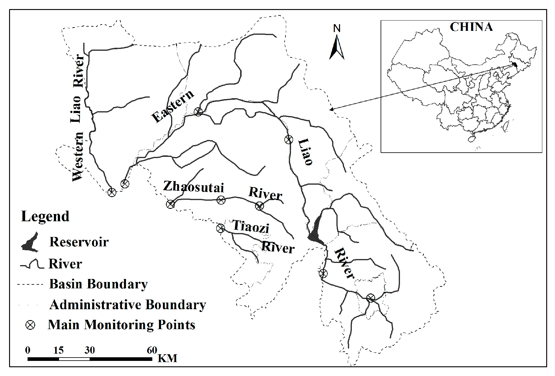
In light of considerable regional differences in water supply and demand, water pollution and economic structure, we take the Source Region of the Liao River (SRLR) characterized by heavy water pollution (mainly organic pollution) and water scarcity as the target area to verify the model performance (Figure 2). SRLR is a core area for agriculture and breeding in Jilin Province with a population of 3.61 million in 2010, covering an area of 14,288 km², which has been undergoing rapid economic development without eligible and effective water environmental management. As a result, water quality is deteriorating seriously and not meeting the requirement for surface water function zoning, and the water availability is limiting regional economic development [35].

Figure 2. Map of the target region.

Figure 2. Map of the target region.

3.1. Proposed Policies and Technologies

In view of the environmental and economic features of the target area, the following environmental policies and corresponding technologies will be introduced (Table 1). In order to select appropriate technologies, additional factors, such as applicability, advancement and the popularization potential of technologies, are also considered. The technologies adopted in this model are introduced from Japan and other regions with similar climatic characteristics.

Table 1. Policies and technologies proposed for water pollution control and water supply and demand.

Objective	Policies	Technologies
Water pollution control	Improvement of the sewage and wastewater treatment rate	New sewage treatment technology Combined treatment septic tank Septic Tank A and B technologies
	Resource-oriented policy for the livestock breeding industry	Biogas power generation technology New fertilizer production technology
	Promotion of forestation and grassland restoration
	Promotion of new fertilizer utilization	Organic-inorganic compound fertilizer Slow-release fertilizer
Water supply and demand	Promotion of reclaimed water production and utilization	Reclaimed water production technology
	Implementation of a multistep water price

Table 1. Policies and technologies proposed for water pollution control and water supply and demand.

Objective	Policies	Technologies
Water pollution control	Improvement of the sewage and wastewater treatment rate	New sewage treatment technology Combined treatment septic tank Septic Tank A and B technologies
	Resource-oriented policy for the livestock breeding industry	Biogas power generation technology New fertilizer production technology
	Promotion of forestation and grassland restoration
	Promotion of new fertilizer utilization	Organic-inorganic compound fertilizer Slow-release fertilizer
Water supply and demand	Promotion of reclaimed water production and utilization	Reclaimed water production technology
	Implementation of a multistep water price

3.2. Data Presentation

The socio-economic and environmental data of the target area are set respectively for the details. The data of the socio-economy in 2010 is derived from the Statistical Yearbook of Jilin Province, Siping City and Liaoyuan City [36,37,38], along with an 11-sector input-output table, which is aggregated based on a 144-sector IO table of 2010. The table considers the pollution characteristics of the target area and the limitations of data accessibility, including private and government consumption, investment, net export and sectoral production. Other economic coefficients, such as the indirect tax rate, the income rate, the value added rate, etc., are determined with data provided by the IO table (Table 2). Land use (Table 2) data are acquired from thematic mapper images through an unsupervised classification and visual interpretation method based on ERDAS 9.2 and ARCGIS 10.0 software.

Table 2. Classification of industries and land use.

Code	Industry	Land use
1	Fishery	Paddy field
2	Growing of rice	Dry land
3	Growing of cereals, leguminous crops and others	Woodland
4	Breeding of pigs	Construction and resident land
5	Breeding of cattle	Grassland
6	Breeding of other livestock and poultry	Other types
7	Mining
8	Manufacturing
9	Construction
10	Production and supply of electricity and gas
13	Transportation, service, etc.

Table 2. Classification of industries and land use.

Code	Industry	Land use
1	Fishery	Paddy field
2	Growing of rice	Dry land
3	Growing of cereals, leguminous crops and others	Woodland
4	Breeding of pigs	Construction and resident land
5	Breeding of cattle	Grassland
6	Breeding of other livestock and poultry	Other types
7	Mining
8	Manufacturing
9	Construction
10	Production and supply of electricity and gas
13	Transportation, service, etc.

The data of water availability and the freshwater consumption coefficients of each sector are collected and calculated based on the Siping and Liaoyuan Water Bulletins [39,40]. According to the organic pollution characteristics in the study area, the total nitrogen (TN), the total phosphorus (TP) and the chemical oxygen demand (COD) are selected as the water pollution indicators. Water pollutant discharge coefficients are calculated with environmental statistical data [41,42]. The GHG emission coefficient of each industry is calculated with the data of the consumption from all kinds of primary and secondary energy of each industry obtained from the Siping and Liaoyuan Statistical Yearbook. Agricultural GHG emission coefficients are calculated with reference to IPCC [43] and Xu et al. [44].

3.3. Constraints and Scenarios Setting

The optimal set of policies is supposed to be formed by meeting the constraints of many preset aspects. According to the local water environmental development plan, the water pollutant discharge constraint is defined as: 30% COD reduction, 30% TN reduction and 25% TP reduction by 2020 compared with 2010. It is assumed that the total reduction amount is allocated into the 10-year simulation horizon. Another constraint is the freshwater supply for socio-economic development, which is decided by the construction of water supply projects and allowable groundwater withdrawal. Other constraints are the proportion of the annual budget from the local government for policy implementation, the restriction of arable land for ensuring food security, the utilization rate of livestock manure from centralized breeding, the treatment rate of urban wastewater, the industrial restructuring direction, etc.

The simulation will be driven by the objective function of the maximization of GRP and operated in several scenarios based on the constraints and policies introduced (Table 3). Scenario 0 (S0) is set as “business as usual” to predict the trend of sectoral economic development, water pollutant discharge, water demand and energy consumption. Due to the presumed linearity between the amount of water pollutants and sectoral production, the reduction of the water pollutant amount could only be achieved with sectoral production decrease when no policies are introduced, which will cause a decrease of the total GRP inevitably. Based on this premise, only sectoral production variation is introduced into Scenario 1 (S1) to detect if the total control of the water pollutant discharge could be achieved. Scenario 2 (S2) is set based on S1 with the introduction of the proposed policies and technologies for water pollution control along with sectoral production variation under the water pollutant discharge constraint. The water availability constraint is introduced in Scenario 3 (S3) based on S2 to uncover how these will further influence the sectoral production. In Scenario 4 (S4), the policies for promoting the water supply and demand balance are additionally introduced based on S3 to clarify the effects on the economic development trend and industrial restructuring brought about by the policies introduced under both the water pollutant discharge constraint and the water availability constraint.

Table 3. Scenario setting in simulation.

Scenarios	Water pollutant discharge constraint	Water availability constraint	Policies for water pollution control	Policy for water supply and consumption
Scenario 0	×	×	×	×
Scenario 1	√	×	×	×
Scenario 2	√	×	√	×
Scenario 3	√	√	√	×
Scenario 4	√	√	√	√

Table 3. Scenario setting in simulation.

Scenarios	Water pollutant discharge constraint	Water availability constraint	Policies for water pollution control	Policy for water supply and consumption
Scenario 0	×	×	×	×
Scenario 1	√	×	×	×
Scenario 2	√	×	√	×
Scenario 3	√	√	√	×
Scenario 4	√	√	√	√

3.4. Model Validation

The simulated results of GRP, water pollutant discharge amount and fresh water demand from 2010 to 2013 for S0 are selected as the indexes to validate the accuracy and feasibility of the model. The comparison of simulated results and actual data indicates that the deviations of GRP, water pollutant discharge amount and freshwater demand are between ±1.5%, ±2.0% and ±2.2%, respectively, which proves the accuracy and feasibility of the model.

4. Results

4.1. Economic Development

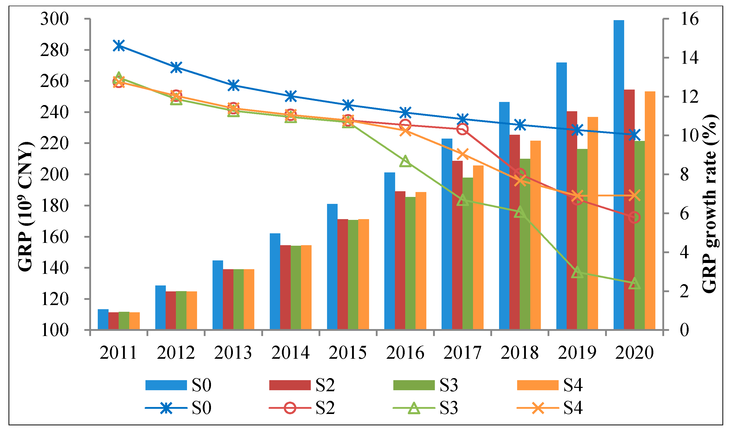
No feasible solution could be found for achieving the water pollutant discharge targets only with sectoral production variation for S1. Because of the introduction of the water pollutant discharge constraint and the freshwater availability constraint, the average GRP growth rate of S2, S3 and S4 decreases to 9.61%, 7.91% and 9.55% from the 11.39% of S0 (Figure 3). During the initial five years, the GRP growth rates of S2, S3 and S4 are similar. However, with a stricter pollutant discharge constraint and greater freshwater demand, a slower growth trend of GRP appears from the sixth year. For S2, with the pollutant discharge constraint getting stricter, the formed policy combination could not help to maintain the GRP growth rate at a high level; hence, a drastic decrease in the GRP growth rate occurs from 2018. The additional introduction of the freshwater availability constraint for S3 incurs an earlier decrease of the GRP growth rate from 2016. The policies for reducing the gap between water supply and water demand in S4 allow the maintenance of the GRP growth rate at a relatively higher level compared with S3.

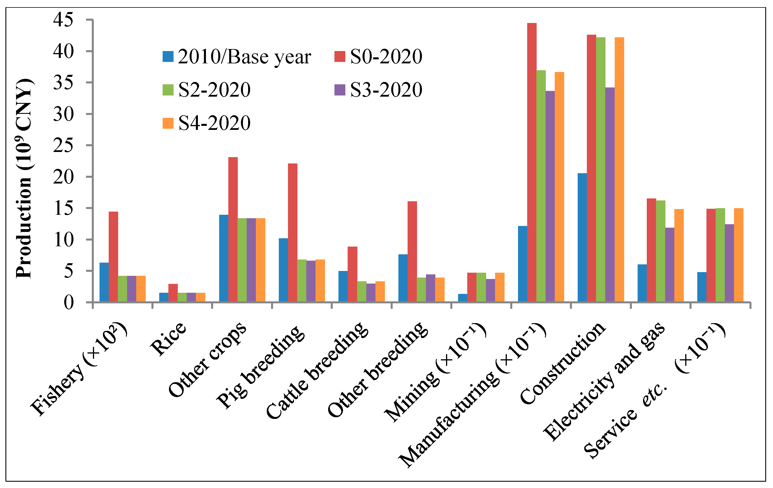
The comparison of each sector’s output for 2020 in each scenario with that of 2010 (base year) is illustrated in Figure 4. The output of each sector increases remarkably by 2020 compared with 2010, especially for the manufacturing, service and mining industries in S0. For S2, the output of fishery and breeding industries, which have larger pollutant discharge coefficients, decreases substantially compared with 2010 (

Table A1. Sectoral coefficients of water pollutant discharge and freshwater consumption.

Sectors	Water pollutant discharge coefficients (Kg/106 CNY)			Freshwater consumption coefficients (m3/106 CNY)
	TN	TP	COD
Fishery	704.32	167.23	1713.44	463,055.11
Growing of rice	1180.37	181.62	2828.39	366,810.39
Growing of cereals, leguminous crops and others	1080.37	151.62	656.44	9584.44
Breeding of pigs	528.27	132.83	2148.58	2408.48
Breeding of cattle	4770.22	497.59	11,047.59	4490.89
Breeding of other livestock and poultry	619.65	223.36	1769.26	2044.28
Mining	2.81	0.03	39.96	681.63
Manufacturing	42.62	5.93	225.80	583.60
Construction	0.23	0.03	4.30	608.19
Production and supply of electricity and gas	3.21	0.04	28.92	13,348.71
Transportation, service etc.	0.11	0.02	0.32	492.80

). The output of farming industries does not decrease much, owing to the national grain production security constraint (food security). The output of manufacturing increases compared with 2010; however, it decreases by 17% compared with S0. This indicates that when the output of the sectors with relatively larger pollutant discharge coefficients has decreased to the lowest limit of industrial development deployed by the local government, if the pollutant discharge targets have not been met, the output of the sectors with relatively smaller pollutant discharge coefficients decreases (Table A1). For S3, when the water availability constraint is additionally introduced, the output of electricity production, manufacturing and construction decreases further compared with S2. For S4, the output of each sector changes little compared with S2, except the electricity production industry with the higher freshwater consumption coefficient (Table A1). This means that the introduced reclaimed water policy and staged water price policy largely mitigate the impacts on industrial development caused by the water availability constraint.

Figure 3. Gross regional product (GRP) trend and the GRP growth rate trend from 2001 to 2020. S0, Scenario 0.

Figure 3. Gross regional product (GRP) trend and the GRP growth rate trend from 2001 to 2020. S0, Scenario 0.

Figure 4. Sectoral output comparison of the scenarios in 2020.

Figure 4. Sectoral output comparison of the scenarios in 2020.

4.2. Water Pollutant Discharge and Abatement

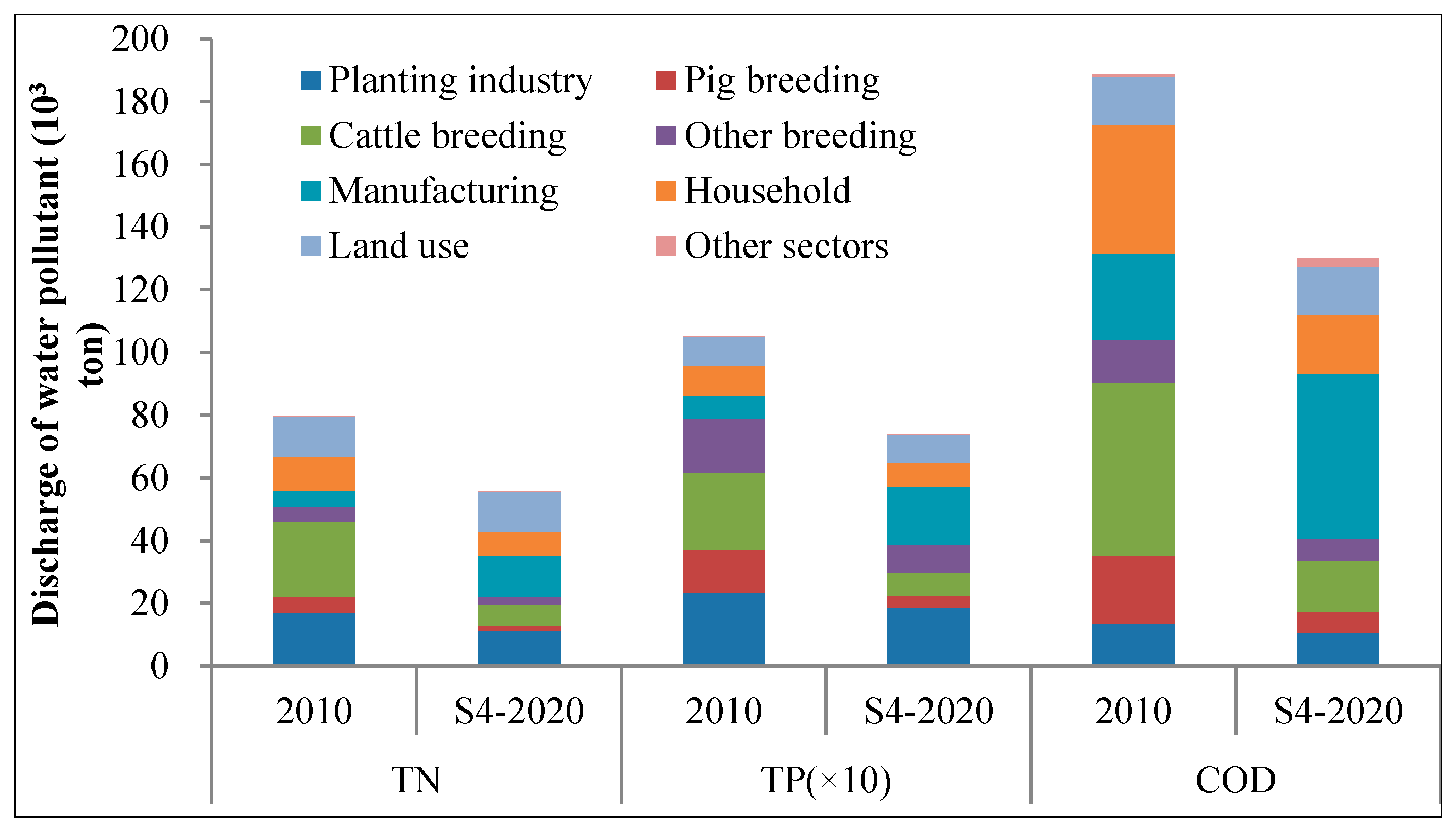
An optimal set of policies have been formed by the model. As shown by Figure 5, the amount of TN, TP and COD reduces to 30.0%, 9.6% and 31.2% by 2020 compared with 2010. Pollutants generated from breeding industries and households reduce drastically in S4. Due to the rapid development of manufacturing, the discharged COD increases once, and TN and TP increase more than once. Almost no change in the discharge amount from land use happens, because the reduced pollutants contributed by the recovery of forestry land and grassland are offset by the increased pollutants caused by the expansion of construction and resident land. The reduction of pollutants is facilitated jointly by sectoral production variation and the introduced policies for water pollution control (Table 4). For planting, pig and cattle breeding, the policy introduction contributes more than 80% and 52% to the pollutant reduction. For manufacturing, the amount of pollutants reduced through the policy introduction is less than that increased by the industrial development, consequently leading to the pollutant increase. On the contrary, for households, the amount of pollutants reduced through the policy introduction is much larger than that increased by the population increase, consequently leading to pollutant reduction.

Figure 5. Water pollutant discharge variation of 2020 in S4 compared with 2010.

Figure 5. Water pollutant discharge variation of 2020 in S4 compared with 2010.

Table 4. Distribution of the contribution of water pollution control in S4.

Sector	Water pollutant discharge variation (ton) caused
	TN		TP		COD
	Production variation	Policy introduced	Production variation	Policy introduced	Production variation	Policy introduced
Fishery	−14.82	0.00	−3.52	0.00	−36.04	0.00
Rice	−17.82	−482.01	−2.29	−45.52	−42.70	−709.50
Other crops	−591.73	−4419.38	−83.04	−346.40	−359.54	−1641.67
Pig breeding	−1798.13	−1976.92	−452.14	−509.56	−7313.38	−7953.85
Cattle breeding	−7975.18	−9019.46	−831.91	−933.53	−18,470.10	−20,219.51
Other breeding	−2288.58	0.00	−824.93	0.00	−6534.43	0.00
Mining	95.07	0.00	1.13	0.00	1354.79	0.00
Manufacturing	10,448.81	−2648.76	1454.95	−299.42	55,378.70	−29,481.09
Construction	4.98	0.00	0.74	0.00	93.06	0.00
Electricity and gas	28.21	0.00	0.31	0.00	254.18	0.00
Service, etc.	30.11	0.00	5.62	0.00	92.33	0.00
Household	661.22 *	−3898.42	55.02 *	−287.04	2926.39 *	−25,113.31
Land use	0.00	−12.12	0.00	−6.71	0.00	1.85
Total	−1436.85	−22,457.06	−683.56	−2428.19	27,283.25	−85,117.07

* Water pollutant discharge variation induced by population increase.

Table 4. Distribution of the contribution of water pollution control in S4.

Sector	Water pollutant discharge variation (ton) caused
	TN		TP		COD
	Production variation	Policy introduced	Production variation	Policy introduced	Production variation	Policy introduced
Fishery	−14.82	0.00	−3.52	0.00	−36.04	0.00
Rice	−17.82	−482.01	−2.29	−45.52	−42.70	−709.50
Other crops	−591.73	−4419.38	−83.04	−346.40	−359.54	−1641.67
Pig breeding	−1798.13	−1976.92	−452.14	−509.56	−7313.38	−7953.85
Cattle breeding	−7975.18	−9019.46	−831.91	−933.53	−18,470.10	−20,219.51
Other breeding	−2288.58	0.00	−824.93	0.00	−6534.43	0.00
Mining	95.07	0.00	1.13	0.00	1354.79	0.00
Manufacturing	10,448.81	−2648.76	1454.95	−299.42	55,378.70	−29,481.09
Construction	4.98	0.00	0.74	0.00	93.06	0.00
Electricity and gas	28.21	0.00	0.31	0.00	254.18	0.00
Service, etc.	30.11	0.00	5.62	0.00	92.33	0.00
Household	661.22 *	−3898.42	55.02 *	−287.04	2926.39 *	−25,113.31
Land use	0.00	−12.12	0.00	−6.71	0.00	1.85
Total	−1436.85	−22,457.06	−683.56	−2428.19	27,283.25	−85,117.07

* Water pollutant discharge variation induced by population increase.

4.3. Water Supply and Demand

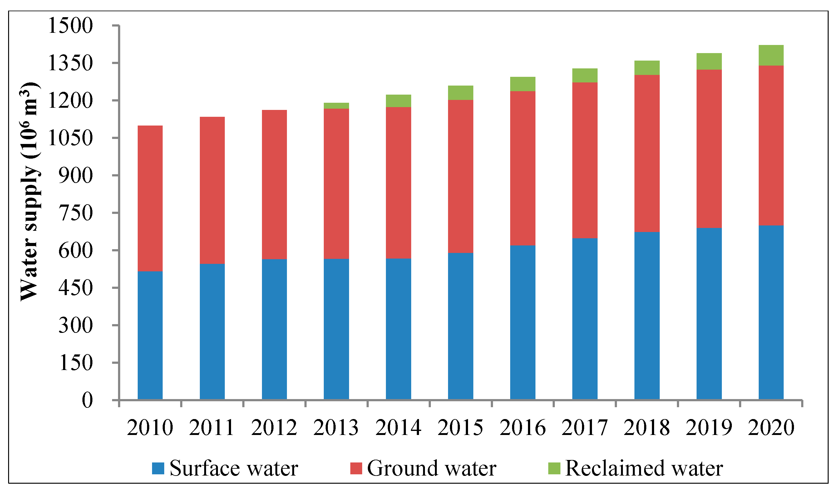
This study mainly considers direct freshwater supply from surface water and ground water without rainfall, which supplies water to crops. Transferred water is also not involved, because no water transfer projects have been put into use before 2020. The water supply trend of S4 is depicted in Figure 6. With the water supply ability being strengthened by the construction of surface water and ground water projects, total water supply is increasing annually. From 2013, since the water resources cannot meet the socioeconomic development requirements, reclaimed water starts to mitigate the scarcity of water resources, accounting for more and more of the total water supply annually. By 2020, the total amount of reclaimed water is 80.26 million m³, accounting for 5.56% of the total water supply.

Figure 6. Direct water supply trend from 2011 to 2020 in S4.

Figure 6. Direct water supply trend from 2011 to 2020 in S4.

Trends of direct water demand for all sectors from 2011 to 2020 are shown in Table 5. From 2011 to 2020, water demand for fishery, planting and breeding industries deceases continuously due to the decrease in sectoral production; water demand for construction, mining, electricity production (thermal power generation) and service industries increases more than once; household water demand increases mainly due to the population increase. In this study, a multistep water price policy specifying a three-order water price system with a ratio of 1:1.5:2 is introduced for urban households. The policy contributes to a decrease of 10.04 million m³ in urban water demand compared with when no policy is introduced in 2020 [45].

Table 5. Trends of the direct water demand of all sectors from 2011 to 2020 in S4 (unit: 10⁶ m³).

Sector	2011	2012	2013	2014	2015	2016	2017	2018	2019	2020
Fishery	27.90	26.78	25.71	24.68	23.70	22.75	21.84	20.97	20.13	19.32
Rice	555.67	555.11	554.56	554.00	553.45	552.90	552.34	551.79	551.24	550.69
Other crops	133.08	132.55	132.02	131.49	130.97	130.44	129.92	129.40	128.88	128.37
Pig breeding	23.56	22.62	21.72	20.85	20.02	19.22	18.46	17.72	17.02	16.34
Cattle breeding	21.48	20.63	19.80	19.02	18.26	17.53	16.83	16.16	15.52	14.87
Other husbandry	14.61	13.67	12.80	11.98	11.21	10.49	9.82	9.19	8.60	8.05
Mining	10.70	12.54	14.46	16.51	18.71	21.06	23.56	26.23	29.07	32.09
Manufacturing	84.14	98.30	113.52	129.90	147.58	165.81	181.84	194.06	203.77	213.96
Construction	13.47	14.49	15.56	16.71	17.95	19.28	20.71	22.24	23.89	25.65
Electricity and gas	91.11	101.80	113.03	125.06	137.94	150.04	161.54	172.96	185.07	198.02
Service etc.	27.21	31.01	34.95	39.20	43.80	48.79	54.21	60.09	66.48	73.41
Household	119.28	119.80	120.31	120.83	121.35	121.87	122.38	122.90	123.42	123.93
Ecological environment *	10.54	11.10	11.66	12.22	12.77	13.33	13.89	14.45	15.01	15.57
Total	1132.73	1160.40	1190.10	1222.46	1257.69	1293.51	1327.35	1358.17	1388.08	1420.26

* Ecological environment water demands are mainly from rivers, lakes, wetland water supplement and urban afforesting.

Table 5. Trends of the direct water demand of all sectors from 2011 to 2020 in S4 (unit: 10⁶ m³).

Sector	2011	2012	2013	2014	2015	2016	2017	2018	2019	2020
Fishery	27.90	26.78	25.71	24.68	23.70	22.75	21.84	20.97	20.13	19.32
Rice	555.67	555.11	554.56	554.00	553.45	552.90	552.34	551.79	551.24	550.69
Other crops	133.08	132.55	132.02	131.49	130.97	130.44	129.92	129.40	128.88	128.37
Pig breeding	23.56	22.62	21.72	20.85	20.02	19.22	18.46	17.72	17.02	16.34
Cattle breeding	21.48	20.63	19.80	19.02	18.26	17.53	16.83	16.16	15.52	14.87
Other husbandry	14.61	13.67	12.80	11.98	11.21	10.49	9.82	9.19	8.60	8.05
Mining	10.70	12.54	14.46	16.51	18.71	21.06	23.56	26.23	29.07	32.09
Manufacturing	84.14	98.30	113.52	129.90	147.58	165.81	181.84	194.06	203.77	213.96
Construction	13.47	14.49	15.56	16.71	17.95	19.28	20.71	22.24	23.89	25.65
Electricity and gas	91.11	101.80	113.03	125.06	137.94	150.04	161.54	172.96	185.07	198.02
Service etc.	27.21	31.01	34.95	39.20	43.80	48.79	54.21	60.09	66.48	73.41
Household	119.28	119.80	120.31	120.83	121.35	121.87	122.38	122.90	123.42	123.93
Ecological environment *	10.54	11.10	11.66	12.22	12.77	13.33	13.89	14.45	15.01	15.57
Total	1132.73	1160.40	1190.10	1222.46	1257.69	1293.51	1327.35	1358.17	1388.08	1420.26

* Ecological environment water demands are mainly from rivers, lakes, wetland water supplement and urban afforesting.

4.4. Policy and Technology Application

All policies are implemented under government control via the introduction of subsidies, which give incentives to stakeholders who consume water resources and discharge water pollutants. The financial sources for each policy consist of the local government budget (LGB), the provincial and central government budget (PCGB) and additional investment from institutional investors with a proportion able to obtain an acceptable profit from new projects, such as biomass energy plants and fertilizer plants (see Formula (18)). The introduced policies are selected and allocated by the simulation model according to distinct levels of pollutant abatement efficiency (cost for the reduction of a unit of pollutant) of technologies (Figure 8b), the subsidization ratio of the local government and the central and provincial government. 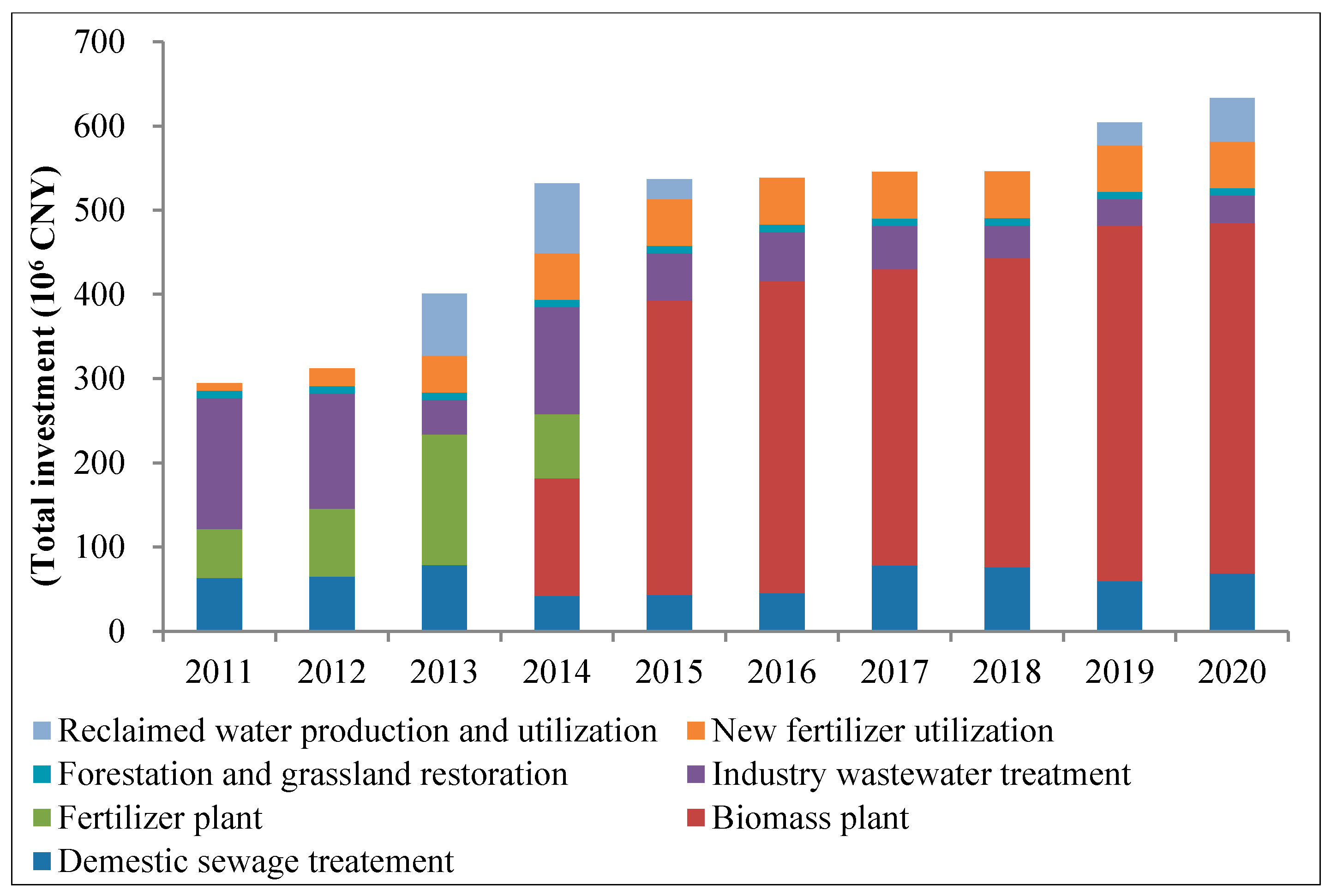Figure 7 depicts the changing trend of total investment for each policy and technology in S4. New fertilizer plants are developed as a priority during the initial years, owing to the lower cost for removing pollutants compared with biomass energy plants. However, from 2015, when all produced fertilizers could meet the requirements of planting, subsidies stop increasing, resulting in no further subsidized investment to fertilizer plants. Contrarily, more livestock excrement is utilized by biomass plants, which increase rapidly after 2014.

Figure 7. Total investment trends for policy or technology from 2011 to 2020 in S4.

Figure 7. Total investment trends for policy or technology from 2011 to 2020 in S4.

During the whole simulation time horizon, the accumulated subsidies for project construction and policy implementation or the operation of projects in S4 are shown in Table 6. The model selects the one that has the best integration treatment performance on pollutants from abatement technologies for one pollution source, which could be presented by the following: when treating rural domestic sewage, Septic Tank B technology is adopted, but not Septic Tank A technology; a new sewage treatment plant adopts demand aeration tank-intermittent aeration tank tecnology and double membrane bio-reactor technology (which are adopted for the production of reclaimed water after wastewater is treated), but not membrane bio-reactor technology. The subsidies for domestic wastewater treatment technologies are determined by the applicable population and treatment capacity per unit cost for each technology simultaneously. Even with the higher cost for removing pollutants, the forestation and grassland restoration policy is propelled by the government especially. For the utilization of new fertilizer, the model determines that slow-release fertilizer is selected for paddy and that organic-inorganic compound fertilizer is applied to other crops. Because the current water price (2.1~2.4 CNY/m³) of the target region is lower than the full cost water price and affordability water price, the government does not subsidize households [46]. Figure 8 indicates the reduction amount and abetment efficiency of each pollutant contributed by each policy or technology. The reduction amount of each pollutant is determined jointly by the amount of subsidies allocated and the reduction efficiency.

Table 6. Subsidization distribution in whole simulation horizon in S4. LGB, local government budget; PCGB, provincial and central government budget; PPA~PWS, denote the corresponding policy or technology in the same row.

Code	Policy or technology	Subsidization and investment (106 CNY)
		Construction			Maintenance
		From LGB	From PCGB	Total investment	From LGB
PPA	Technology upgrade and pipe construction for old sewage treatment plant	47.13	31.42	78.55	146.34
PPB	New sewage treatment plant and pipe construction for urban household	54.39	36.26	90.65	19.76
PPC	Combined treatment septic tank for urban household	24.15	16.10	40.26	7.75
PPD	Septic Tank B for rural household	287.17	123.07	410.25	61.21
PPE	New sewage treatment plant and pipe construction for industry	301.31	75.33	753.28 #	0.00
PPF	Biogas power generation plant for centralized pig breeding	269.14	134.57	672.85 *	101.49
PPG	Biogas power generation plant for centralized cattle breeding	698.20	349.10	1,745.51 *	201.89
PPH	New fertilizer plant for centralized pig breeding	55.80	25.40	141.99 *	0.00
PPI	New fertilizer plant for centralized cattle breeding	91.82	48.41	227.05 *	0.00
PPJ	Promotion of woodland restoration	28.22	7.06	35.28	0.00
PPK	Promotion of grassland restoration	41.95	10.49	52.43	0.00
PPL	Promotion of new fertilizers utilization for rice growing	44.78	29.85	74.63	0.00
PPM	Promotion of new fertilizers utilization for other crops growing	231.80	154.53	386.34	0.00
PWR	Reclaimed water production and supply system	180.27	77.26	257.53	0.00
PWS	Staged water price for urban household	0.00	0.00	0.00	0.00

* Including investment from institutional investors; ^# Including investment from enterprises that discharge wastewater into the treatment plant.

Table 6. Subsidization distribution in whole simulation horizon in S4. LGB, local government budget; PCGB, provincial and central government budget; PPA~PWS, denote the corresponding policy or technology in the same row.

Code	Policy or technology	Subsidization and investment (106 CNY)
		Construction			Maintenance
		From LGB	From PCGB	Total investment	From LGB
PPA	Technology upgrade and pipe construction for old sewage treatment plant	47.13	31.42	78.55	146.34
PPB	New sewage treatment plant and pipe construction for urban household	54.39	36.26	90.65	19.76
PPC	Combined treatment septic tank for urban household	24.15	16.10	40.26	7.75
PPD	Septic Tank B for rural household	287.17	123.07	410.25	61.21
PPE	New sewage treatment plant and pipe construction for industry	301.31	75.33	753.28 #	0.00
PPF	Biogas power generation plant for centralized pig breeding	269.14	134.57	672.85 *	101.49
PPG	Biogas power generation plant for centralized cattle breeding	698.20	349.10	1,745.51 *	201.89
PPH	New fertilizer plant for centralized pig breeding	55.80	25.40	141.99 *	0.00
PPI	New fertilizer plant for centralized cattle breeding	91.82	48.41	227.05 *	0.00
PPJ	Promotion of woodland restoration	28.22	7.06	35.28	0.00
PPK	Promotion of grassland restoration	41.95	10.49	52.43	0.00
PPL	Promotion of new fertilizers utilization for rice growing	44.78	29.85	74.63	0.00
PPM	Promotion of new fertilizers utilization for other crops growing	231.80	154.53	386.34	0.00
PWR	Reclaimed water production and supply system	180.27	77.26	257.53	0.00
PWS	Staged water price for urban household	0.00	0.00	0.00	0.00

* Including investment from institutional investors; ^# Including investment from enterprises that discharge wastewater into the treatment plant.

Figure 8. Pollutant reduction amount (a) and reduction efficiency (b) contributed by each policy or technology.

Figure 8. Pollutant reduction amount (a) and reduction efficiency (b) contributed by each policy or technology.

4.5. Energy and GHGs Emission

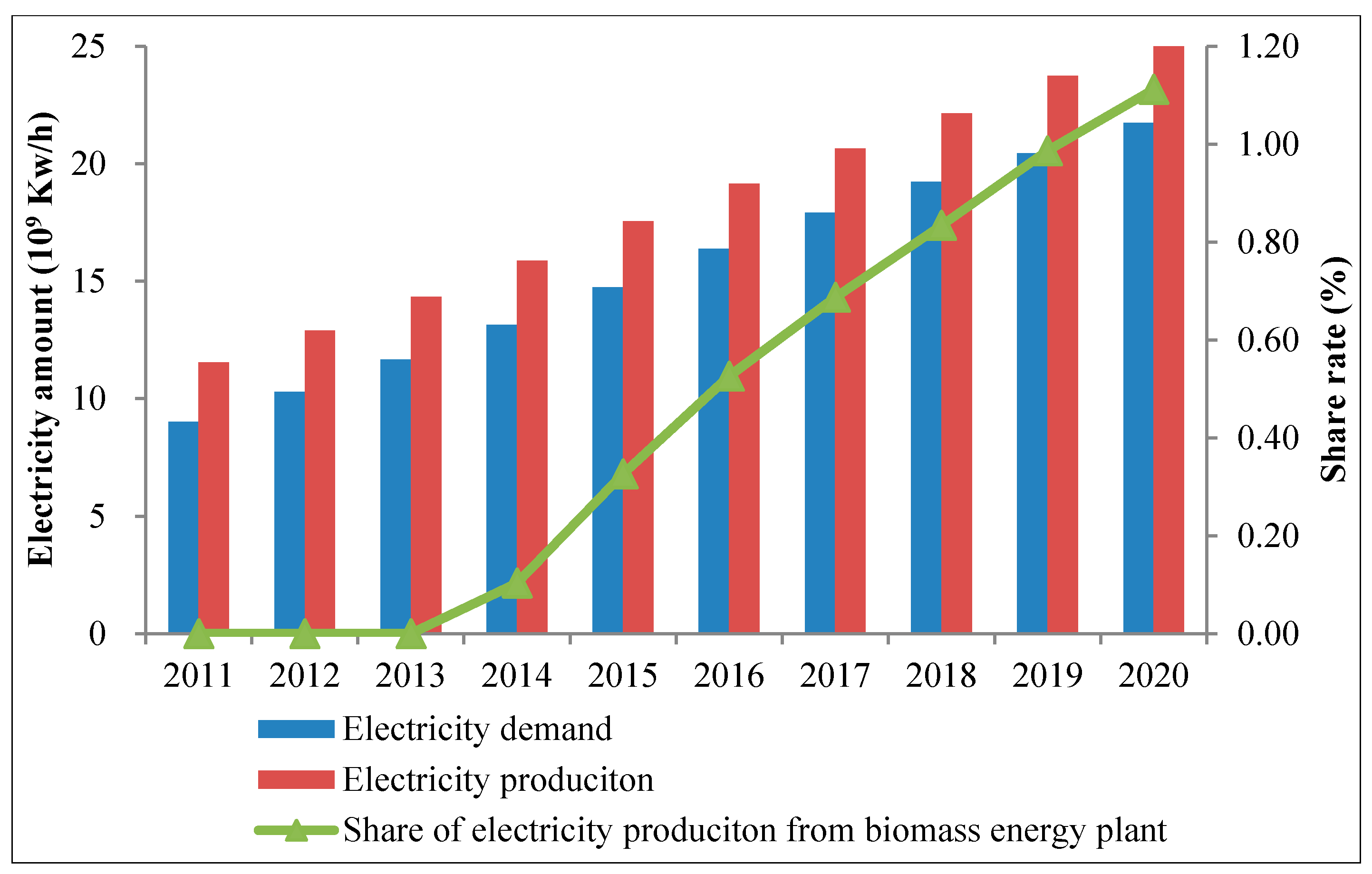
When introducing policies for reducing pollutants from breeding industries, a biomass energy plant is proposed to treat livestock excrement with electricity generated, which indirectly contributes to electricity production and supply. Figure 9 shows the increasing trend in electricity demand and production of the target area with the electricity demand proportion increasing from 77.96% in 2010 to 85.43% in 2020 for S4. Biomass energy plants begin to provide electricity from 2014 with the proportion increasing continuously to 1.11% by 2020.

Figure 9. Electricity production trends and supply from 2011 to 2020 in S4.

Figure 9. Electricity production trends and supply from 2011 to 2020 in S4.

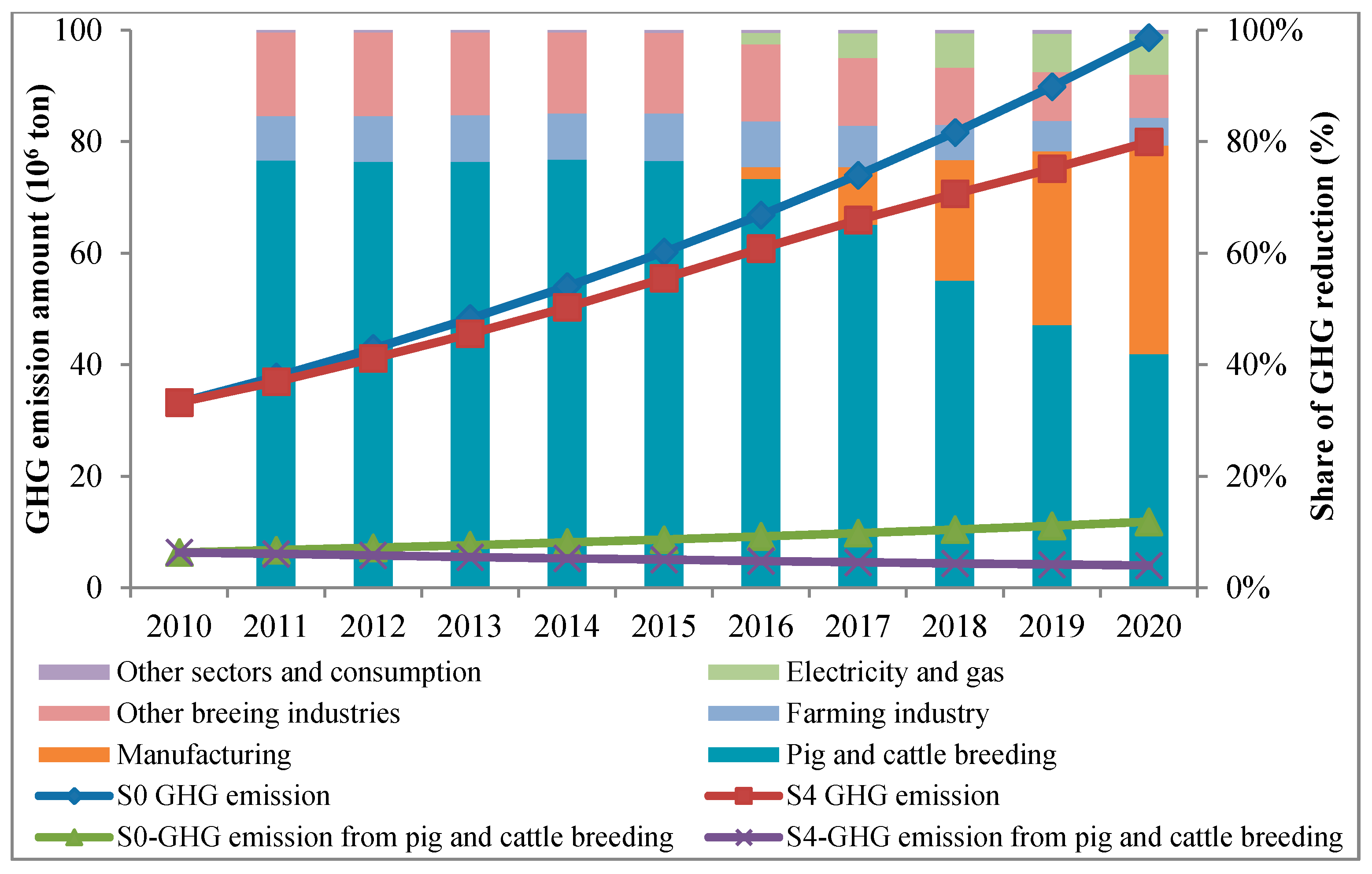
The effects induced by the constraints of pollutant discharge and water availability could be also reflected in GHG emissions. Figure 10 illustrates the contrast in the changing trend of the GHG emission amount between S4 and S0. The GHG emission amount decreases annually in S4 compared with S0, mainly due to the sectoral production decrease. Initially, the largest proportion of GHG emission reduction is accomplished by pig and cattle breeding industries, owing to both the production decrease and livestock excrement treatment; and afterwards, more sectors become the reduction contributors, attributed to the induced production decrease. For S4, for the GHG emissions from the pig and cattle breeding industry, 9.81% of the reduction amount by 2020 compared with 2010 is contributed by livestock excrement treatment, with the remainder contributed by the reduction in the total number of livestock. This is due to the much larger emission amount from livestock rumination than from livestock excrement.

Figure 10. Trend in the GHG emission and GHG reduction contributors.

Figure 10. Trend in the GHG emission and GHG reduction contributors.

5. Summative Discussion

The introduced water pollutant discharge constraint and water availability constraint inevitably bring negative impacts to economic development. These are expected to be mitigated by the newly-proposed water resource utilization policies and water pollution abatement policies to promote the maximization of negative impacts regional economy and ultimately realize regional sustainable development. Such a complex problem is solved within an optimization framework specified by the simulation model through finding the optimal solution to maximize GRP meeting various constraints in four preset scenarios. The contrasts in the four scenarios show that the water pollutant discharge constraint and the water availability constraint incur a continuous annual decrease in GRP when no policies are introduced; the GRP trend could increase with the introduction of policies, but is still lower than the BAU conditions (S0), implying that an optimal set of the integrated policies formed and the sectoral production decrease collectively contribute to meeting the constraints. Specifically, the production decrease of sectors is determined through decreasing the least value added, removing the most water pollutants and reducing water resource consumption after taking the value added rate, the pollutant discharge coefficient and the water consumption coefficient of all sectors into account. More specifically, the production decrease of sectors should be limited to a threshold that ensures the production of a certain sector able to meet the requirements for intermediate demand in related sectors and regional government and private consumption.

As a typical agricultural area, the target region’s water body is mainly polluted due to the extensive use of fertilizers for the planting industry and the large amount of pollutants discharged from the breeding industry. The rapid industrial development and water resource consumption exacerbate the water pollution. The water pollution abatement policies and water resource utilization policies are proposed in view of the environmental pollution characteristics of the target region, and whether they are selected and implemented or not is determined by the simulation. There are a variety of different technologies and policies proposed for joint implementation and/or with different timings for policy planning. The model constructed in this study makes it possible to identify an optimal set of technologies and policies adaptable to the target region and effective at improving the environment with less economic sacrifice of the stakeholders within the river basin.

The selection and implementation of each policy or technology is affected by the following factors set in the model at the same time, and the optimal set of policies is supposed to be formed considering all of the following:

Water pollutant joint-removal efficiency: the costs of different policies or technologies for removing a unit of pollutant are different; the pollutant removal efficiencies of different policies or technologies are different with the same investment.

Limitation of the technology application potential: the potential applicable population for different household sewage treatment technologies; the amount of organic wastes generated from breeding industries; the wastewater amount discharged from manufacturing industry.

Subsidy source and allocation mechanism: In the model, the ratio of the subsidies from the provincial and the central government is an exogenous variable that is set to be fixed for each policy or technology. The amount of subsidies from the local government budget is an endogenous variable determining the total amount of subsidies for new project construction or policy promotion. It is at the same time restricted by local financial revenue, which is closely related to GRP, whose increase will indirectly induce a rise in the subsidy amount. Thus, the optimal balance between the maximization of the GRP and the minimization of pollution is expected to be achieved.

Specific constraints: In the empirical study, some specific constraints based on local or national government policies can be specified into ecological conservation (restoration of forestry and grassland), food security (ensuring a specific area of arable land), the promotion of new and renewable energy (organic wastes utilized as bio-resources for energy production) and the sewage and wastewater treatment rate.

6. Conclusions

A dynamic optimization simulation model has been presented based on IO analysis to form an optimal set of policies, to accomplish total control of water pollutant discharge and the balance of water supply and demand, with minimum negative influence on GRP. An empirical study with the SRLR basin as the target area has been carried out to verify the performance of the model.

The contrasts of four scenarios indicate that the formed optimal policy combination with industrial restructuring collectively achieves the targets of the water pollutant discharge constraint and the water availability constraint. The trends of economic development, pollutant discharge and water consumption for each sector within the simulation time horizon are depicted dynamically through clarifying the industrial restructuring direction, the pollution structure and pollutant discharge amount and the freshwater consumption and supply amount, which are endogenously derived from the model. The extent of the mitigation of water pollution control and water scarcity contributed by the applied policies or technologies and the subsidies granted to promote policy or technology implementation are specified, from which the mechanisms of the policy application and the subsidization allocation are systematically clarified. The policy combination contributes a 94.06% and a 97.81% reduction of TN and TP in 2020 compared with 2010, with the rest contributed by production variation. The former removes 85.12 thousand tons of COD, and the latter increases 27.34 thousand tons of COD. Reclaimed water supply accounts for 5.56% of the total freshwater supply in 2020. Although not including energy structure adjustment policies, the simulation predicts energy supply and demand and the changing trend of the GHG emissions of all sectors. Thus, an optimal level of the relationships among all socio-economic activities is explored and presented by the simulation model.

It has been proven that the optimal set of policies can facilitate the simultaneous pursuit of the mitigation of water pollution and water scarcity and the increase of GRP effectively. The model is robust in the case that once the parameters and necessary data have been input, the model will obtain an optimal solution as a result of the comprehensive and overall evaluation of all of the possible policies and technologies that have been put forward by means of identifying the regional water resources, pollution characteristics and economic structure.

A possible future extension is to introduce industrial technological innovations for the mitigation of pollutant discharge and water resource consumption. The methodology adopted based on IO analysis can be designed to explore the interrelationships between GHG emissions, atmospheric pollutant emissions (SO₂, PM2.5), as well as energy substitution and economic development with industrial restructuring to finally realize the simultaneous sustainable development of the economy, the environment and energy.