Estimating Potential GDP for the Romanian Economy and Assessing the Sustainability of Economic Growth: A Multivariate Filter Approach

Abstract

In the current context of economic recovery and rebalancing, the necessity of modelling and estimating the potential output and output gap emerges in order to assess the quality and sustainability of economic growth, the monetary and fiscal policies, as well as the impact of business cycles. Despite the importance of potential GDP and the output gap, there are difficulties in reliably estimating them, as many of the models proposed in the economic literature are calibrated for developed economies and are based on complex macroeconomic relationships and a long history of robust data, while emerging economies exhibit high volatility. The object of this study is to develop a model in order to estimate the potential GDP and output gap and to assess the sustainability of projected growth using a multivariate filter approach. This trend estimation technique is the newest approach proposed by the economic literature and has gained wide acceptance with researchers and practitioners alike, while also being used by the IMF for Romania. The paper will be structured as follows. We first discuss the theoretical background of the model. The second section focuses on an analysis of the Romanian economy for the 1995–2013 time frame, while also providing a forecast for 2014–2017 and an assessment of the sustainability of Romania’s economic growth. The third section sums up the results and concludes.

1. Introduction

During the current period of transition, the Romanian economy has experienced several structural disequilibria and has exhibited high macroeconomic volatility. Structural reform has been initiated and partially completed over the past decade and, together with sustained foreign capital inflow and the transfer of technology, has fueled economic growth prior to the onset of the financial crisis in 2008. At the same time, the decline in the manufacturing industry has led to the erosion of industrial capital and to rising rates of unemployment.

Studies by the IMF (International Monetary Fund) [1,2,3,4] show that the rapid growth of the Romanian economy in the expansionary period was mainly due to total factor productivity in 2000–2006, while in the last two years before the crisis (2007 and 2008), growth was supported by the capital stock in the economy. It is worth noting that the contribution of labor to economic growth has not been significant, with the exception of the years 2006 and 2007. The background of these macroeconomic developments was the sustained increase in direct investment backed by foreign credit. The economic downturn of 2009 and 2010 was due chiefly to financial disintermediation and the severe decline in total factor productivity, with the latter only exhibiting sluggish recovery after 2011. During this period, foreign investment in the Romanian economy declined drastically, as a result of local banks’ tightening lending policies due to limited funding from their parent institutions, who also faced severe financial issues in their core markets. The consequences on the Romanian economy were severe, with a record number of small and medium enterprises going bankrupt, a significant delay in capital investment in the economy (investment was postponed until economic recovery) and the capital stock becoming obsolete, all of these factors impacting economic growth. These developments have been accompanied by increasing rates of unemployment and erosion of human capital, thus affecting potential economic growth [2,5,6].

Based on the history of 88 banking crises that occurred over the past four decades, a study by the IMF [6] shows that there is a shift in potential output subsequent to the crisis, with potential GDP (gross domestic product) falling below pre-crisis levels. This happens because financial systems that are affected by the crises take long to heal, and this imposes further restrictions on lending and investment in the economy. At the same time, the rise of unemployment during recessions can negatively impact structural unemployment, but this depends to a great extent on the flexibility of the labor market and the goods and services markets, which may lead to a quicker and more cost-effective relocation of the labor force between industries as opposed to rigid systems. In emerging economies, the growth potential is additionally constrained by the worsening sustainability of public debt and the weakness of state budgets due to the elimination of fiscal stimuli and foreign capital repatriation.

Under these circumstances, estimating potential GDP is a cumbersome challenge that involves a great deal of uncertainty. It is a sensitive issue, because the potential output and output gap are cornerstone economic policy variables, while at the same time being important communication tools of the monetary and political authorities [7].

Given the actual and perceived importance of the measures of economic output, developing appropriate and reliable measurement tools is of great benefit to both economic researchers and practitioners. This paper focuses on the design of a multivariate filter model to be used in the estimation of the potential GDP and output gap for the Romanian economy. Our model is based on macroeconomic relationships that have been validated, both theoretically, as well as empirically during the transition of the Romanian economy to a full-fledged market-based system. The model shall be used retrospectively, for the Q1 1995–Q3 2014 time horizon, as well as prospectively, in order to produce forecasts for the 2014–2017 time frame. Technically, the model can be used to generate projections over a longer horizon; however, this involves a great deal of uncertainty and the risk of compounding forecast errors, given the relatively high volatility of the Romanian economy ([8]). As such, we consider that the 2014–2017 time frame is a conservatively appropriate forecast horizon.

As we shall see, an important advantage of our model is that it can be used to assess the sustainability of economic growth. By linking measures of the potential GDP and output gap to fundamental macroeconomic variables and their equilibrium states and by incorporating their laws of dynamics, the model explicitly takes into account the impact of other macroeconomic gaps (i.e., in manufacturing capacity utilization, unemployment and inflation) on the quality and sustainability of projected growth.

2. Experimental Section

In its most abstract definition, potential GDP represents the level of output consistent with the aggregate supply of the economy in the long run after cyclical (short-term) macroeconomic shocks have dissipated. Potential output is fundamental to the Phillips curve, which states the inverse relationship between inflation and unemployment. When actual GDP rises above its potential (equilibrium) level, the economy is overheated and inflationary pressures amplify; when output falls below its equilibrium level, the economy faces the risk of disinflation.

Potential GDP is defined as the level of aggregate supply that attains the optimum balance between output and price stability, given full employment [9,10,11]. An alternative definition of potential GDP is the level of output that is achievable given the existing capital stock and labor input if the economy were neither in expansion nor in recession. It is therefore clear that the potential GDP and the output gap are key variables for macroeconomic policies; however, employing them in the decision making process has been troublesome due to both unreliable estimation models and varying intensities of the fluctuations of other macroeconomic variables [12]. Other authors define potential GDP as the maximum output that an economy could sustain without generating inflationary pressures [13].

In spite of the classical filtering techniques (e.g., Hodrick–Prescott and Kalman filters—see [14,15,16,17,18]) enjoying great popularity with practitioners and academics alike, these methods have the important limitation of ignoring fundamental macroeconomic relationships, and this is a key fact to consider in the case of emerging economies ([19]). For instance, in many countries, the monetary authorities adopt an inflation-targeting regime of monetary policy (with this also being the case in Romania), a policy stance that leads to overly restrictive policy measures during recessions. This, in turn, generates prolonged periods of negative output gaps. If forecasting models failed to account for inflation during the period, they would produce biased estimates of the potential output and output gap. These issues can lead to inappropriate economic policies (please see the discussion in [20] for an accurate depiction of the way in which errors in potential output estimation led to ineffective monetary policies in the United States in the 1970s and the 1980s). It is also compulsory to update estimates as new information on macroeconomic time series becomes available, even if the national accounts are not subject to revision themselves. As discussed in several studies, the issue of updating estimates for the potential GDP and output gap points out that the revisions can be material for recent periods and can create serious issues in the forecasting process [5,21,22,23,24].

In order to overcome the shortcomings of the simple univariate filtering techniques, several models have been proposed that enhance standard filters with information from other macroeconomic variables. The Reserve Bank of New Zealand’s FPS (Forecasting Policy System) model augments a standard HP (Hodrick–Prescott) filter with an inflation gap, an employment gap and a capacity utilization gap [20]. This is done in order to improve the assessment of inflationary pressures in New Zealand and to reduce further revisions as new data become available [5]. Empirical evidence suggests that this model does not necessarily outperform the HP filter, while also highlighting the fact that the model fails to produce accurate forecasts of potential output for more than one quarter ahead [25].

Some authors show that while HP filters perform poorly at estimating the cyclical component of GDP, especially at the end of the sample (which is the period of maximum importance to decision making), enhancing univariate methods with structural relationships does not necessarily improve forecasting accuracy due to the difficulties inherent in model calibration. The authors provide the example of the model used by the Bank of Canada and show that it underperforms the HP filter, citing the additional features introduced to improve the estimates as the most likely reason [26]. Other studies show that it is useful to enhance measures of the real-time output gap with information about capacity utilization rates (e.g., from business surveys) [27]. Evidence from a 22-country panel dataset suggests that incorporating qualitative and quantitative information on capacity utilization rates can produce real-time output gap estimates that are much closer to subsequent estimates (and revisions).

Given the macroeconomic context and the multitude of channels through which the economic crisis made its mark on the global environment, the need for a new approach of estimating potential GDP emerges, a new approach that accounts for conditioning information and relationships relevant to national economies. The multivariate filter approach proposed in [20] is based on an operational definition of equilibrium output, where potential output is the level of GDP that can be sustained over the long run without generating inflation trends. Implicit in this definition is the hypothesis that the inflationary process contains information critical to the estimation of potential output. This is the reason why several researchers have estimated potential GDP using various models of inflation dynamics. However, there is no reason to confine the estimation of equilibrium output by using just inflation as an input; this is why the multivariate filter approach devised in [20] incorporates empirically-observed relationships between actual and potential GDP, the unemployment rate and the NAIRU (non-accelerating inflation rate of unemployment), core inflation and manufacturing capacity utilization.

The inclusion of the output gap in NAIRU models represents a totally different perspective compared with Friedman’s theory [28], according to which NAIRU is not determined by the aggregate demand; however, it is consistent with recent findings [29]. The central argument of Friedman’s proposal is that the natural rate of unemployment depends on the characteristics of the labor market, such as minimum wage, bargaining power of unions and frictions produced by the incompatibility between the unemployed and available jobs, and it cannot be influenced by aggregate demand or monetary policy. At the same time, the author suggests that the natural rate of unemployment can vary in time due to labor market imperfections (an idea backed by other authors, e.g., [30]). Some studies mention productivity slowdown and globalization as arguments for variations in NAIRU over time [31,32], providing the notable example of Europe, where NAIRU rose considerably between 1960 and 2000. Another argument lies in the impact of technological progress on the demand for unqualified labor, which reduces in time [33]. Due to labor market imperfections, there is a certain wage rigidity, such that the effective compensation of unqualified workers does not change, even though the equilibrium wages for this type of work have reduced. The obvious result is an increase in unemployment.

New approaches have been proposed according to which changes in NAIRU are chiefly determined by fluctuations of aggregate demand that affect the current level of unemployment, which, in turn, influences NAIRU through a hysteresis phenomenon [29]. The hysteresis concept was introduced in the 1980s [34] and is based on the following theory of collective wage bargaining: when some employees enter unemployment, the rest of the employees negotiate their wages, and as a result, labor compensation faces upward pressure, thus preventing former employees from getting their jobs back. However, as pointed out in [29], there is no convincing evidence for this type of hysteresis; rather, hysteresis is due to people who have been unemployed over the long term isolating themselves from the labor market: either they are no longer of interest to prospective employers or quit looking for jobs. It is suggested that this effect is more likely to happen in developed economies, where state unemployment benefits are paid over the long term, and that an upward trend of NAIRU is almost always accompanied by a process of disinflation. As for the opposite process of NAIRU reduction, this can be interpreted as a mean reversion tendency or assimilated with an inflationary process [29].

The hysteresis phenomenon also has important implications with respect to the monetary policy, in that it is dangerous for central banks to focus excessively on inflation [29,35]. If we start from the argument that the natural rate of unemployment is independent of monetary policy, then targeting inflation can only produce short-term fluctuations in actual unemployment; however, through the hysteresis effect, these short-term fluctuations will influence NAIRU. In this context, a given inflation target can be consistent with more than one equilibrium rate of unemployment, even in the long run. It is also important to note that a central bank can meet its inflation target, while at the same time creating unnecessary high unemployment. Some authors discuss that in a recession, monetary policy should be expansionary, which does not always happen, with inappropriate monetary policy decisions having the power to amplify the hysteresis phenomenon [35,36].

Apart from incorporating the aforementioned underlying dynamics of NAIRU, a fundamental assumption of the multivariate filter model is that the growth rate of potential output is allowed to vary in time based on information recently acquired, while also giving credit to the trends observed over the long term ([37]).

The multivariate filter model is based on three macroeconomic gaps:

➢

output gap ($y_t$), the log difference between actual GDP actual ($Y_t$) and potential GDP (${\overline{Y}}_t$):

$$y_t=100\ln \frac{Y_t}{{\overline{Y}}_t}$$

(1)

➢

unemployment gap ($u_t$), the difference between the natural unemployment rate (NAIRU, ${\overline{U}}_t$) and the observed actual rate of unemployment ($U_t$):

$$u_t={\overline{U}}_t-U_t$$

(2)

➢

manufacturing capacity utilization gap ($c_t$), the difference between the actual capacity utilization in the manufacturing industry ($C_t$) and its equilibrium value (${\overline{C}}_t$):

$$c_t=C_t-{\overline{C}}_t$$

(3)

Inflation is modelled using a stochastic process that explicitly considers the impact of the output gap and changes in the output gap from the previous period to the current period on core inflation (${\pi }_t$):

$${\pi }_t={\pi }_{t-1}+\alpha \left(y_t-y_{t-1}\right)+\beta y_t+{\epsilon }_t^{\pi }$$

(4)

It is implicit in Equation (4) that the empirical result of a direct relationship between inflation and the output gap is respected; moreover, a change in output gap $\left(y_t-y_{t-1}\right)$ can signal important macroeconomic adjustments. Consider, for example, a positive $y_t$ and a negative variation $\left(y_t-y_{t-1}\right)$ this might well suggest the onset of an economic contraction. Reciprocally, a negative $y_t$ and a positive $\left(y_t-y_{t-1}\right)$ could indicate the end of a recession. The coefficient of the previous period core inflation rate is set to one, because the best expectation for current inflation is the rate of inflation from the previous period. Albeit apparently simple, Equation (4) produces reliable results for many economies and for long time horizons that include one or several changes in the monetary policy regime (see [20] for a detailed discussion).

The following equation is proposed for the dynamics of the unemployment gap (essentially a modified version of Okun’s law [38]):

$$u_t=\gamma u_{t-1}+\delta y_t+{\epsilon }_t^u$$

(5)

whereas the capacity utilization gap is modelled as follows:

$$c_t=\mu c_{t-1}+\nu y_t+{\epsilon }_t^c$$

(6)

Equation (6) is necessary because the manufacturing capacity utilization gap contains valuable information that could serve as an indicator of the output gap, while at the same time being influenced by the output gap: in a recession, we expect the capacity utilization gap to be negative at the same time as the output gap is negative, with the opposite being true for an expansionary period. It should also be noted that, as the recent crisis has shown, cyclical fluctuations in industry have been significantly more volatile than the overall economy, which calls for a value greater than one for $\nu$.

We now focus on the laws of movement for the equilibrium variables. For NAIRU, we shall have the following equation:

$${\overline{U}}_t={\overline{U}}_{t-1}+S_t^{\overline{U}}-\xi y_{t-1}-\psi \left({\overline{U}}_{t-1}-U^{LTE}\right)+{\epsilon }_t^{\overline{U}}$$

(7)

where $U^{LTE}$ denotes the long-term equilibrium unemployment rate; the positive parameters $\xi$ and $\psi$ link NAIRU to the output gap and NAIRU to its deviation from the long-term equilibrium unemployment rate, respectively. An important novelty of the model developed in [20] consists of the explicit inclusion of two types of shocks, here denoted by the random variables $S_t^{\overline{U}}$ (structural, lasting shocks) and ${\epsilon }_t^{\overline{U}}$ (cyclical shocks, with a transitory impact on NAIRU).

The structural shocks in NAIRU ($S_t^{\overline{U}}$) follow an autoregressive process of the following form:

$$S_t^{\overline{U}}=\left(1-\kappa \right)S_{t-1}^{\overline{U}}+{\epsilon }_t^{G^{\overline{U}}}$$

(8)

An aspect worth mentioning here is that the long-term unemployment rate ($U^{LTE}$) is assumed to be constant, even though the model allows for structural shocks in NAIRU. In this context, the appropriate interpretation for NAIRU is a short- and medium-term equilibrium rate of unemployment that will ultimately converge to its long-term steady state. This hypothesis is consistent with the discussion on NAIRU in some studies [39].

The dynamics of potential GDP is modelled using the following equation [20]:

$${\overline{Y}}_t={\overline{Y}}_{t-1}-\omega \left({\overline{U}}_t-{\overline{U}}_{t-1}\right)-\frac{\left(1-\omega \right)\left({\overline{U}}_{t-1}-{\overline{U}}_{t-20}\right)}{19}+\frac{G_t^{\overline{Y}}}{4}+{\epsilon }_t^{\overline{Y}}$$

(9)

where $G_t^{\overline{Y}}$ is the potential GDP growth rate, and fluctuations in NAIRU are linked to potential output through parameter $\omega$, which represents the labor force occupation rate. The 19-quarter change in NAIRU $\left({\overline{U}}_{t-1}-{\overline{U}}_{t-20}\right)$ is intended to capture the effect of changes in the capital stock; the effect of a permanent 1 percentage point (p.p.) increase in NAIRU in one quarter will be a $\omega$ p.p. decrease in potential GDP; this negative effect is expected to continue for another 19 quarters (making up for a 5-year time horizon), such that the total decline in potential GDP is 1%. The potential growth rate $G_t^{\overline{Y}}$ follows an autoregressive process of the form:

$$G_t^{\overline{Y}}=\left(1-\rho G_{t-1}^{\overline{Y}}\right)+\rho G_{LT}^{\overline{Y}}+{\epsilon }_t^{G^{\overline{Y}}}$$

(10)

In which $G_{LT}^{\overline{Y}}$ represents the long-term potential rate of growth in GDP (the steady-state GDP growth rate).

The manufacturing capacity utilization is modelled using a process that includes both persistent, as well as punctual shocks (in a similar fashion to the NAIRU process described in Equation (7)):

$${\overline{C}}_t={\overline{C}}_{t-1}+G_t^{\overline{C}}+{\epsilon }_t^{\overline{C}}$$

(11)

where:

$$G_t^{\overline{C}}=\left(1-\varsigma \right)G_{t-1}^{\overline{C}}+{\epsilon }_t^{G^{\overline{C}}}$$

(12)

As for the long-term inflation expectations, it must be noted that the way in which central banks establish their inflation objectives is not transparent; monetary policies change in time, and it is not always easy to anticipate changes in the monetary policy regime. The most suitable approach for long-term inflation expectations is an adaptive process of the following form [20]:

$${\pi }_t^{LTE}={\pi }_{t-1}^{LTE}+{\epsilon }_t^{{\pi }^{LTE}}$$

(13)

where the residual ${\epsilon }_t^{{\pi }^{LTE}}$ captures the adjustments in inflation expectations from one period to the next. In the context of a regime change or under the circumstances of a monetary policy that does not target inflation directly, ${\epsilon }_t^{{\pi }^{LTE}}$ can be substantial; however, as the recent experience of developed economies has shown, inflation objectives have been relatively stable, thus rendering ${\epsilon }_t^{{\pi }^{LTE}}$ almost negligible for these economies [20].

The output gap equation considers both the previous value of this gap, as well as the fluctuations of the inflation rate versus its target value:

$$y_t={\theta }_1{y}_{t-1}-{\theta }_2\left({\pi }_t-{\pi }_t^{LTE}\right)+{\epsilon }_t^y$$

(14)

which is consistent with the traditional approach to monetary policy in which any deviations of the inflation rate from its target are corrected by adjusting the reference rate, which of course influences the output gap. In periods of high inflation due to excess demand, central banks turn to a restrictive monetary policy, which reduces the output gap. All other factors that influence the output gap (e.g., aggregate demand shocks) are captured by the residual ${\epsilon }_t^y$.

As discussed to some extent by the IMF [2], the sustainability of economic growth cannot be assessed in the absence of the previously discussed relationships between output gap and the other fundamental gaps (in unemployment, capacity utilization and inflation). Romania’s significant growth experience in 2004–2008, mainly due to foreign-financed credit and the transfer of technology, has not been accompanied by a strengthening of the macroeconomic fundamentals, and as such, the ensuing recession has had a severe impact on the Romanian economy. It is our contention that sustainable economic growth can only happen in the context of strong fundamentals, with critical macroeconomic variables at or near their equilibrium levels.

The next step in model calibration is the estimation of parameters (posteriors). For this purpose, we use the Bayesian technique of maximum regularized likelihood, as discussed in [40]. This estimation technique allows for the specification of prior distributions for the parameters in order for the model to produce reasonable results. The objective function of the algorithm is:

$$\underset{\vartheta }{\max }=\ln L\left(\vartheta ,X\right)-p{\displaystyle \sum _i\frac{{\left({\vartheta }_i-{\overline{\vartheta }}_i\right)}^2}{{\sigma }_{{\overline{\vartheta }}_i}^2}}$$

(15)

where $\vartheta$ is the parameter vector to be estimated, X is the data vector and L is the likelihood function. The assumption here is that the prior distribution of each parameter is normal with mode ${\overline{\vartheta }}_i$ and variance $\frac{1}{p}{\sigma }_{{\overline{\vartheta }}_i}^2$, with the parameter estimates being the mode of their posterior distribution, as calculated in the optimization process. The following additional restriction is necessary:

$${\vartheta }_i\in \left[{\vartheta }_i^L,{\vartheta }_i^U\right]$$

(16)

where the lower and upper bounds are provided by the user in order to produce reliable parameter estimates.

Before proceeding with the estimation of the model, we want to stress that there is evidence in the literature that multivariate filters do not necessarily perform better than simple detrending methods (e.g., the HP filter), nor do they warrant less frequent subsequent revisions of estimates [25]. An additional issue is the length of the time series used in the calibration of the models. The author shows that a seven-year time span for New Zealand’s economy is likely to lead to unreliable results. However, uncertainty is also induced when models are expanded to incorporate long time horizons of 40–50 years: revisions to the measures of the output gap can be substantial, sometimes exceeding six percentage points [22,41,42]. Of course, this can lead to erroneous monetary policy decisions if too much emphasis is placed on the output gap.

A side benefit of the multivariate filter models is that they are generally better at predicting inflation rather than at predicting the output gap itself [25]. However, discussing the practical usefulness of the output gap concept, some authors show that while in theory, the output gap might be useful to understand the inflationary pressures in the economy, in practice, it is difficult to do this, because it is inherently difficult to estimate the output gap in real time; that is, when decisions are made that affect the future [43]. This applies in the case of both univariate and multivariate filters. The authors also highlight that, regardless of the model used, it is very difficult to identify shifts in the cycle in real time (the so-called “end-point problem”). When these shifts are eventually discovered, the prior estimates of potential GDP must be revised to take into account this conditioning information. The added complexity and uncertainty inherent in multivariate models may well offset the benefits of including theoretically useful information from other macroeconomic variables and their laws of movement.

3. Results and Discussion

In this section, we aim at calibrating the multivariate filter model in order to derive estimates of the potential output and output gap for Romania. Prior to estimating the model, two important assumptions need to be made. Firstly, in order to ensure that the growth rate of potential GDP does not deviate significantly from its steady state, we shall impose the following additional constraint:

$$4\cdot \left({\overline{Y}}_t-{\overline{Y}}_{t-1}\right)=G_{LT}^{\overline{Y}}+{\epsilon }_t$$

(17)

where the residual ${\epsilon }_t$ captures our prior estimates of the volatility of growth in potential output in relation to its long-term equilibrium value (steady state) $G_{LT}^{\overline{Y}}$. Of course, in the case of developed economies, the residual ${\epsilon }_t$ may be negligible, as the rate of growth in potential GDP is fairly stable. However, in the case of emerging economies, with significant short-term fluctuations of macroeconomic variables and the high impact of business cycles on the growth potential of the economy, a higher prior standard deviation for ${\epsilon }_t$ is warranted. The prior volatility of ${\epsilon }_t$ should be set to equal one-third of the standard deviation of the actual real GDP growth rate [20].

The second important assumption concerns parameter p in the objective function Equation (15). The lower the value of the parameter, the more significant the impact of the priors on the optimization procedure. A value of p equal to one is suggested, which implies a neutral perspective on the prior probability distributions of the parameters [20]. This is also the choice for the model to be calibrated in our study.

Before running the model, we make the following methodological clarifications. The time series for actual real GDP (reference year 2000) and unemployment span over the period Q1 1995–Q3 2014 and have been obtained from the Romanian National Institute of Statistics and Eurostat. Actual and core inflation and capacity utilization rates have been retrieved from the Eurostat database and cover the periods Q1 1996–Q3 2014, Q4 2000–Q3 2014 and Q1 2001–Q3 2014, respectively. For long-term inflation expectations, we used IMF estimates for the 1995–2010 horizon and the National Bank of Romania’s inflation target for 2011–2014.

At this point, one may raise a justified concern as to the validity of the model with only 79 quarters of data available, i.e., almost 20 years. While in the case of developed economies, longer data series are used, often exceeding 30 years, it must be stated that lack of data availability and relatively low data reliability are an important issue in the case of Romania. Moreover, the multivariate filter model is based on data spanning from Q1 1992 to Q4 2010, i.e., 19 years. The model has been calibrated and estimations have been performed using the MATLAB R2010a software and code originally developed and published by the authors of [20] and available online at [44].

Our model differs from the approach in [20] in several ways. Firstly, rather than relying on somewhat arbitrary long-term inflation expectations, it aligns long-term inflation expectations with the inflation target of the National Bank of Romania (from 2011 onwards). In our view, this is warranted by the very nature of the central bank policy and by the fact that NBR’s (National Bank of Romania) annual target is flat at 2.5% starting 2013. Secondly, we dropped the 1992–1994 period, as there is significant uncertainty in the data due to sparse availability of the time series. In the third place, the parameter priors have been adjusted by expert judgment, so as to account for the inherently higher volatility of the Romanian economy compared to developed countries (for which the model in [20] was initially calibrated).

Table 1 below presents the steady states of the model. These are consistent with the approach in [2], with the sole exception of the long-term potential GDP growth rate $G_{LT}^{\overline{Y}}$, for which we set a less conservative value (3.8%, as opposed to the IMF estimate of 3.7%), due to the positive evolution of the Romanian economy in the Q4 2012–Q3 2014 time frame. In our opinion, the increase in productivity over this horizon warrants a higher potential GDP growth rate in the long run.

Table 1. The steady states of the model. Source: [2], authors’ assumptions.

Parameter	Equilibrium Value
Potential GDP growth rate ($G_{LT}^{\overline{Y}}$)	3.80%
Labor force participation rate ($\omega$)	0.70
Long-term unemployment rate ($U^{LTE}$)	6.00%

Table 1. The steady states of the model. Source: [2], authors’ assumptions.

Parameter	Equilibrium Value
Potential GDP growth rate ($G_{LT}^{\overline{Y}}$)	3.80%
Labor force participation rate ($\omega$)	0.70
Long-term unemployment rate ($U^{LTE}$)	6.00%

Another important input for the multivariate model is the set of prior distributions for the parameters, as previously discussed. A set of priors is suggested in [20] for several developed countries (the United States, Germany, Great Britain, France, Italy, Canada, the Euro Area, Australia, Norway, New Zealand, Spain and China), which we shall also use as a starting point, with the mention that the prior standard deviations of each parameter have been increased by 5% in order to better reflect the higher volatility of the Romanian economy. We also want to stress that for the standard deviations of the residuals in the potential GDP Equation (9) and its growth rate (Equation (10)), we used our own estimates. The priors and posteriors for each of the model’s parameters are presented in Table 2.

An important advantage of the multivariate filter lies in the fact that the model makes use of Bayesian techniques to simultaneously estimate fundamental macroeconomic relationships, with the output gap being derived as the common factor that drives all macroeconomic variables sensitive to the business cycle, such as unemployment, inflation and capacity utilization. The results of running the model for the Romanian economy over the Q1 1995–Q3 2014 time horizon are given in Table 3 (potential output, output gap, unemployment gap and manufacturing capacity utilization gap):

Table 2. The prior and posterior distributions of the parameters. Source: adjusted values originally proposed in [20] and our own estimates.

Parameter	Prior		Posterior		Parameter	Prior		Posterior
	Mode	Variance	Mode	Mode		Mode	Variance	Mode	Variance
α	0.400	0.331	0.299	0.047	θ2	5.000	3.308	4.800	0.489
β	0.500	0.331	0.447	0.047	$\sigma \left({\epsilon }_t^{\pi }\right)$	0.500	0.331	1.510	0.039
γ	0.800	0.165	0.784	0.024	$\sigma \left({\epsilon }_t^u\right)$	0.500	0.331	1.153	0.039
δ	0.300	0.165	0.258	0.024	$\sigma \left({\epsilon }_t^c\right)$	0.400	0.331	1.283	0.040
μ	0.100	0.662	0.167	0.077	$\sigma \left({\epsilon }_t^{\overline{U}}\right)$	0.100	0.165	0.293	0.024
ν	1.500	1.654	0.931	0.147	$\sigma \left({\epsilon }_t^{\overline{U}}\right)$	0.100	0.165	0.304	0.025
ξ	3.000	1.654	2.953	0.244	$\sigma \left({\epsilon }_t^{\overline{Y}}\right)$	0.050	0.126	0.330	0.014
ψ	2.000	3.308	2.057	0.473	$\sigma \left({\epsilon }_t^y\right)$	1.000	0.331	2.382	0.050
κ	0.900	0.165	0.898	0.024	$\sigma \left({\epsilon }_t^{\overline{C}}\right)$	0.250	0.110	0.723	0.016
ρ	0.100	0.165	0.037	0.016	$\sigma \left({\epsilon }_t^{G^{\overline{C}}}\right)$	0.075	0.033	0.209	0.005
$\varsigma$	0.500	0.165	0.498	0.025	$\sigma \left({\epsilon }_t^{{\pi }^{LTE}}\right)$	0.300	0.300	0.325	0.016
θ1	0.800	0.165	0.800	0.023	$\sigma \left({\epsilon }_t^{\overline{Y}}\right)$	0.013	0.032	0.037	0.005

Table 2. The prior and posterior distributions of the parameters. Source: adjusted values originally proposed in [20] and our own estimates.

Parameter	Prior		Posterior		Parameter	Prior		Posterior
	Mode	Variance	Mode	Mode		Mode	Variance	Mode	Variance
α	0.400	0.331	0.299	0.047	θ2	5.000	3.308	4.800	0.489
β	0.500	0.331	0.447	0.047	$\sigma \left({\epsilon }_t^{\pi }\right)$	0.500	0.331	1.510	0.039
γ	0.800	0.165	0.784	0.024	$\sigma \left({\epsilon }_t^u\right)$	0.500	0.331	1.153	0.039
δ	0.300	0.165	0.258	0.024	$\sigma \left({\epsilon }_t^c\right)$	0.400	0.331	1.283	0.040
μ	0.100	0.662	0.167	0.077	$\sigma \left({\epsilon }_t^{\overline{U}}\right)$	0.100	0.165	0.293	0.024
ν	1.500	1.654	0.931	0.147	$\sigma \left({\epsilon }_t^{\overline{U}}\right)$	0.100	0.165	0.304	0.025
ξ	3.000	1.654	2.953	0.244	$\sigma \left({\epsilon }_t^{\overline{Y}}\right)$	0.050	0.126	0.330	0.014
ψ	2.000	3.308	2.057	0.473	$\sigma \left({\epsilon }_t^y\right)$	1.000	0.331	2.382	0.050
κ	0.900	0.165	0.898	0.024	$\sigma \left({\epsilon }_t^{\overline{C}}\right)$	0.250	0.110	0.723	0.016
ρ	0.100	0.165	0.037	0.016	$\sigma \left({\epsilon }_t^{G^{\overline{C}}}\right)$	0.075	0.033	0.209	0.005
$\varsigma$	0.500	0.165	0.498	0.025	$\sigma \left({\epsilon }_t^{{\pi }^{LTE}}\right)$	0.300	0.300	0.325	0.016
θ1	0.800	0.165	0.800	0.023	$\sigma \left({\epsilon }_t^{\overline{Y}}\right)$	0.013	0.032	0.037	0.005

Table 3. Potential GDP and output gap. Source: [2,3], AMECO, authors’ calculations. MV, multivariate filters; EC, European Commission; AMECO, Annual Macro-Economic Database; IMF, International Monetary Fund.

bn. RON	2002	2003	2004	2005	2006	2007	2008	2009	2010	2011	2012	2013
Real GDP	89.8	94.6	102.0	106.9	115.4	123.3	133.5	124.3	123.3	124.6	125.5	129.4
Pot. GDP (MV)	91.6	96.7	102.9	109.4	115.8	121.9	126.7	127.7	126.7	126.0	127.3	129.9
Gap (MV)	−2.0%	−2.2%	−0.8%	−2.3%	−0.3%	1.1%	5.5%	−2.7%	−2.7%	−1.2%	−1.4%	−0.4%
Gap (EC)	−0.7%	1.1%	4.9%	4.4%	5.9%	7.0%	9.0%	−0.3%	−2.6%	−3.1%	−4.1%	−2.4%
Gap (IMF)	−2.4%	−3.0%	−1.1%	−1.6%	0.9%	3.0%	6.2%	1.5%	−1.5%	−1.2%	−2.4%	−1.2%

Table 3. Potential GDP and output gap. Source: [2,3], AMECO, authors’ calculations. MV, multivariate filters; EC, European Commission; AMECO, Annual Macro-Economic Database; IMF, International Monetary Fund.

bn. RON	2002	2003	2004	2005	2006	2007	2008	2009	2010	2011	2012	2013
Real GDP	89.8	94.6	102.0	106.9	115.4	123.3	133.5	124.3	123.3	124.6	125.5	129.4
Pot. GDP (MV)	91.6	96.7	102.9	109.4	115.8	121.9	126.7	127.7	126.7	126.0	127.3	129.9
Gap (MV)	−2.0%	−2.2%	−0.8%	−2.3%	−0.3%	1.1%	5.5%	−2.7%	−2.7%	−1.2%	−1.4%	−0.4%
Gap (EC)	−0.7%	1.1%	4.9%	4.4%	5.9%	7.0%	9.0%	−0.3%	−2.6%	−3.1%	−4.1%	−2.4%
Gap (IMF)	−2.4%	−3.0%	−1.1%	−1.6%	0.9%	3.0%	6.2%	1.5%	−1.5%	−1.2%	−2.4%	−1.2%

The model’s results are consistent with the evolution of the Romanian economy over the 1995–2014 time horizon. As shown in Figure 1 below, after a period of hyperinflationary growth, the Romanian economy has been characterized by weak productivity and external competitiveness, which together with capacity underutilization in the industry have led to a negative output gap in the first part of the last decade (2000–2004). In real terms, the economy grew; however, actual growth was below potential growth, and the (negative) output gap did not close. The fluctuations in the output gap in the 2005–2006 time frame, in the context of sustained economic growth, can be partly attributed to the change in the monetary policy regime in Romania, with the National Bank switching to an inflation targeting regime that requires a close correlation of the reference rate with inflation expectations (and with the expected output gap evolution, for that matter).

Figure 1. A multivariate filter estimation of Romania’s principal macroeconomic gaps. Source: authors’ calculations.

Figure 1. A multivariate filter estimation of Romania’s principal macroeconomic gaps. Source: authors’ calculations.

The sustained real economic growth continued in 2007 and 2008, when, due to a hike in total factor productivity and industrial capacity utilization, increasing external competitiveness and decreasing unemployment, the output gap closed and the economy subsequently overheated, growing much faster than implied by its potential rate of growth. With the onset of the crisis at the end of 2008, Romania experienced economic contraction for two successive years (a decrease of 6.9% in 2009 and 0.8% in 2010). During the recession, the National Bank of Romania, fearing inflation, had been reluctant to cut the reference rate, whereas foreign investment reduced drastically and the banking system faced soaring rates of non-performing loans (with the end-2008 liquidity crisis on top), and has thus been reluctant to finance the real economy. These developments have naturally led to a negative output gap and to a much more moderate potential GDP growth rate. Romania’s economic recovery, at first weak and due to external factors, such as exceptional performance in agriculture (2011) and the pleasant surprises of 2013 and the first three quarters of 2014, have brought GDP on a track consistent with its potential level, thus narrowing the output gap. It is worth mentioning that the potential GDP growth rate has slowed down compared to pre-crisis levels, mostly as a result of Romania’s structural weakness during the crisis, the increasing burden of public debt and the sluggish recovery of internal demand subsequent to the recession, thus raising question marks as to the sustainability of prospective economic growth.

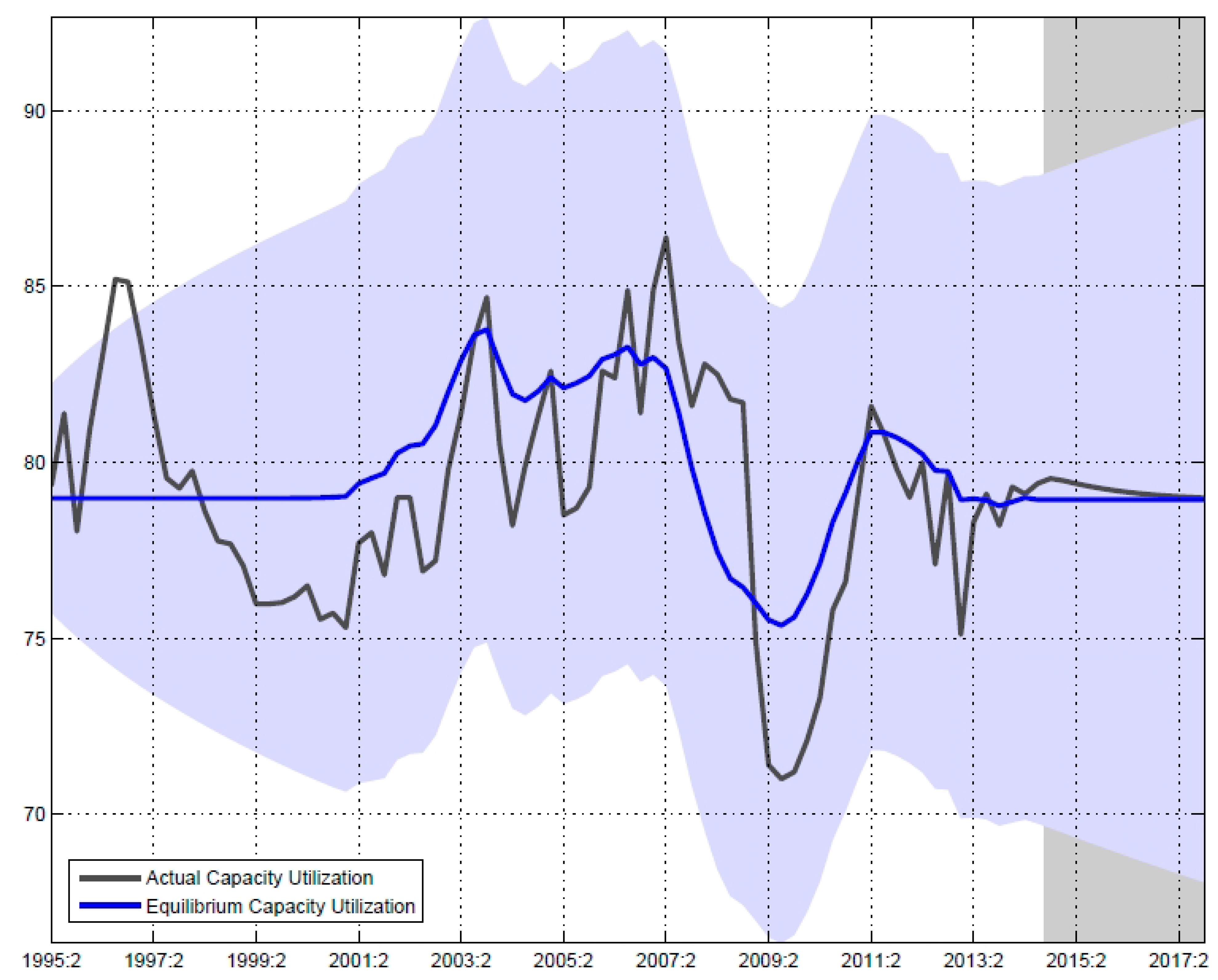
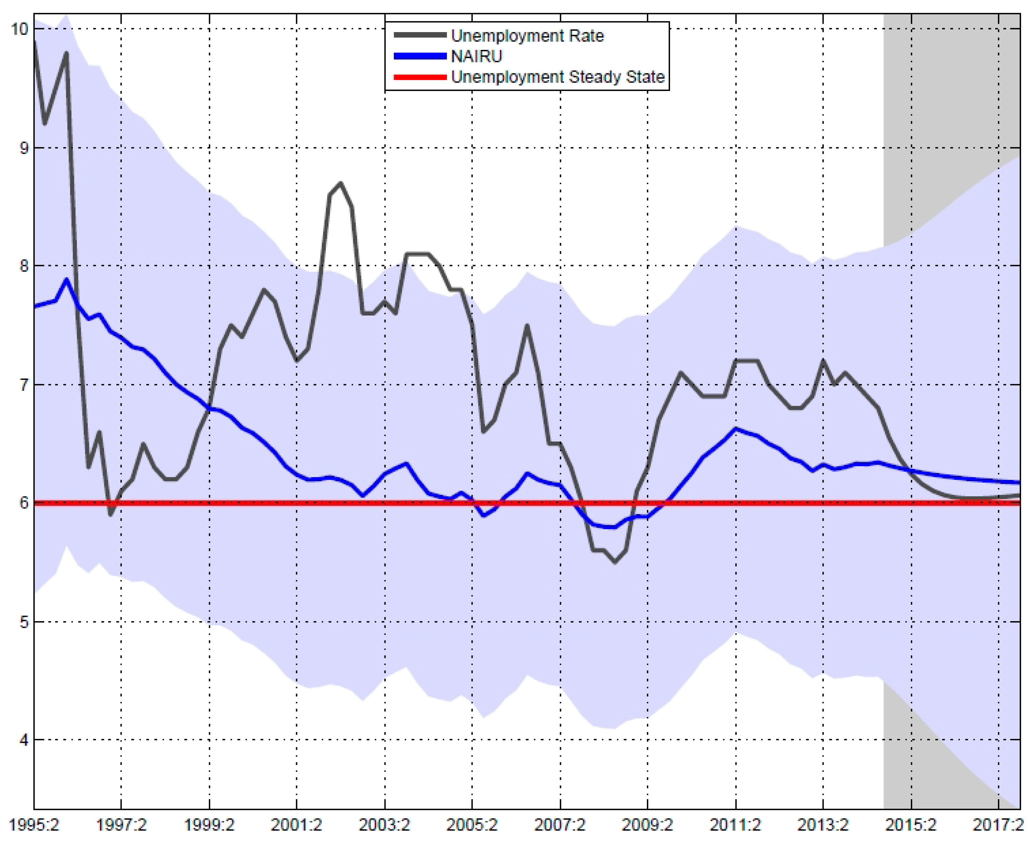
It is interesting that the model captures accurately the effects of the economic crisis on industrial capacity utilization, which exhibited a negative gap in the 2009–2013 time frame due to the slow recapitalization of the Romanian economy and weak dynamics of capital investment during the economic recession (please see Figure 2). The output gap was closely followed by the manufacturing capacity utilization gap, and it took five years for both gaps to close. The unemployment gap has been negative over the whole period as a result of the increase in NAIRU due to the hysteresis effect and the increase in actual (cyclical) unemployment during the crisis; however, as the economy rebounds and grows above its potential level (starting 2015), the model predicts a drop in unemployment, thus reducing the unemployment gap in 2015–2017 and bringing the unemployment rate and NAIRU on a trend consistent with the steady state of unemployment in the Romanian economy, as depicted in Figure 3 below.

Figure 2. Evolution of the manufacturing capacity utilization. Source: authors’ calculations. The light blue area represents a ±2 standard deviation confidence interval for equilibrium capacity utilization.

Figure 2. Evolution of the manufacturing capacity utilization. Source: authors’ calculations. The light blue area represents a ±2 standard deviation confidence interval for equilibrium capacity utilization.

Figure 3. Evolution of NAIRU and the unemployment rate. Source: authors’ calculations. The light blue area represents a ±2 standard deviation confidence interval for NAIRU.

Figure 3. Evolution of NAIRU and the unemployment rate. Source: authors’ calculations. The light blue area represents a ±2 standard deviation confidence interval for NAIRU.

Let us now turn our attention to the relationship between the output gap and the inflation rate, which is of substantial relevance to a monetary policy regime that explicitly targets inflation. Until 2005 (the moment when NBR changed its monetary policy regime), the output gap and the inflation rate were largely uncorrelated; however, subsequent to 2005, the correlation between the two variables is obvious, as shown in Figure 4 below. The inflation rate continued on its descending path in 2005–2006, when the output gap was still negative, but rose sharply in 2007–2008, when the economy overheated and the gap turned positive. The crisis meant that the output gap turned negative again, and as expected, the inflation rate declined during this period. The closing of the output gap in 2014–2015 and the subsequent expected economic growth will likely result in the convergence of inflation to its steady state: with actual output near its potential level in the foreseeable future; and in the current economic context (low euro area inflation and low oil prices), inflationary pressures are not likely to threaten the Romanian economy.

Figure 4. The evolution of inflation and output gap. Source: authors’ calculations. The light blue area represents a ±2 standard deviation confidence interval for the output gap.

Figure 4. The evolution of inflation and output gap. Source: authors’ calculations. The light blue area represents a ±2 standard deviation confidence interval for the output gap.

We now propose a comparison between the results produced by our multivariate filter approach and the latest IMF estimates for Romania. In addition, in order to assess the relative performance of the multivariate filter model, we have also included the results of an HP filter estimation, using a parameter λ = 1600 and the same quarterly real GDP data series. Table 4 below gives the output gap and the expected potential GDP growth rate for the interval 2004–2014, as well as forecasts for 2014–2017.

Table 4. The evolution of the output gap and potential GDP growth rate (Pot. Gr. Rate). Source: [2,3], authors’ estimates. HP, Hodrick–Prescott.

YEAR, %	2004	2005	2006	2007	2008	2009	2010	2011	2012	2013	2014	2015	2016	2017
Gap (MV)	−0.8	−2.3	−0.3	1.1	5.5	−2.7	−2.7	−1.2	−1.4	−0.4	0.3	0.4	0.2	0.1
Gap (HP)	0.4	−1.2	0.6	2.6	7.7	−1.2	−2.6	−1.9	−1.9	0.1	n.a	n.a	n.a	n.a
Gap (IMF)	−1.1	−1.6	0.9	3.0	6.2	1.5	−1.5	−1.2	−2.4	−1.2	−1.2	−1.2	−0.9	−0.2
Pot. Gr. Rate (MV)	6.4	6.3	5.8	5.3	3.8	0.9	−0.8	−0.5	1.0	2.0	2.3	2.6	2.8	2.9
Pot. Gr. Rate (HP)	6.5	6.5	6.0	4.8	3.1	1.5	0.5	0.4	0.7	1.0	n.a	n.a	n.a	n.a
Pot. Gr. Rate (IMF)	6.0	5.5	4.8	4.3	3.4	2.2	1.9	1.8	2.0	2.2	2.3	2.5	2.6	2.6

Table 4. The evolution of the output gap and potential GDP growth rate (Pot. Gr. Rate). Source: [2,3], authors’ estimates. HP, Hodrick–Prescott.

YEAR, %	2004	2005	2006	2007	2008	2009	2010	2011	2012	2013	2014	2015	2016	2017
Gap (MV)	−0.8	−2.3	−0.3	1.1	5.5	−2.7	−2.7	−1.2	−1.4	−0.4	0.3	0.4	0.2	0.1
Gap (HP)	0.4	−1.2	0.6	2.6	7.7	−1.2	−2.6	−1.9	−1.9	0.1	n.a	n.a	n.a	n.a
Gap (IMF)	−1.1	−1.6	0.9	3.0	6.2	1.5	−1.5	−1.2	−2.4	−1.2	−1.2	−1.2	−0.9	−0.2
Pot. Gr. Rate (MV)	6.4	6.3	5.8	5.3	3.8	0.9	−0.8	−0.5	1.0	2.0	2.3	2.6	2.8	2.9
Pot. Gr. Rate (HP)	6.5	6.5	6.0	4.8	3.1	1.5	0.5	0.4	0.7	1.0	n.a	n.a	n.a	n.a
Pot. Gr. Rate (IMF)	6.0	5.5	4.8	4.3	3.4	2.2	1.9	1.8	2.0	2.2	2.3	2.5	2.6	2.6

The economic crisis has had a significant impact on the Romanian economy, cutting its growth potential significantly. The latest IMF estimates (as of March 2014) point at a potential GDP growth rate of 2%–2.3% until 2014 and up to 2.6% in 2017, in the context of a negative output gap over the entire horizon (albeit effectively closing at −0.2% in 2017). By incorporating the positive results from Q4 2012–Q3 2014, mostly due to the revival of consumption and investment in the Romanian economy, our model yields more optimistic estimates, with the output gap expected to close in 2014–2015 and a quicker recovery of economic growth, up to a rate of 2.9% in 2017. However, this all is to be taken with a grain of salt: if structural reform and capital investment in the Romanian economy do not accelerate, our forecast might be too optimistic, with growth rates hitting pre-target levels only after 2017–2018 and short-term economic growth risking becoming unsustainable.

As expected, due to its linear nature, the HP filter produces results that are quite different from those of the multivariate filter. At the same time, they are arguably somewhat unrealistic: the estimations indicate that potential GDP grew in the midst of the crisis, by 1.5% in 2009 and 0.5% in 2010; this is hard to believe, considering the severe impact of the recession on the Romanian economy.

In order to gauge the relative performance of the HP and MV (multivariate filters) filters, we must define a quantitative criterion against which the two models can be judged. Our approach is consistent with that discussed in some studies [25], in that the better model is the one that is less prone to revisions as future data become available. We proceed as follows: first, we estimate potential GDP using the data up to Q4 2012, and then, we perform estimations for each subsequent quarter until Q3 2014. Afterwards, we calculate the mean of RMSEs (root mean square error) for 1, 2, 3 and 4-step ahead estimates for both the MV and HP filters. The results are given in Table 5.

The MV filter delivers consistently better results than the HP filter. When one quarter of new information becomes available, the MV filter outperforms the HP filter by 38%; the difference grows bigger when more than at least two quarters of data are added, exceeding 70%. In the case of the highly volatile Romanian economy, this was to be expected, as the HP filter produces estimates that fail to account for complex macroeconomic relationships. The results in Table 5 also indicate that the HP filter performs poorly as a forecast tool compared to the MV filter, and its performance gets worse when forecasting over longer time horizons due to the compounding of errors. As such, policy makers should treat the results of the HP filter with caution and, if possible, use them in conjunction with the outputs of competing models.

Table 5. The relative performance of the MV and HP filters. Source: authors’ estimates.

Mean RMSE	Quarters Ahead
Method	1	2	3	4
MV Filter	0.1552%	0.6268%	0.1419%	0.1826%
HP Filter	0.2138%	1.0662%	0.2553%	0.3164%
Increase in Mean RMSE HP vs. MV	38%	70%	80%	73%

Table 5. The relative performance of the MV and HP filters. Source: authors’ estimates.

Mean RMSE	Quarters Ahead
Method	1	2	3	4
MV Filter	0.1552%	0.6268%	0.1419%	0.1826%
HP Filter	0.2138%	1.0662%	0.2553%	0.3164%
Increase in Mean RMSE HP vs. MV	38%	70%	80%	73%

Figure 5 illustrates real GDP growth and potential GDP growth as estimated by the multivariate filter. The Romanian economy grew faster than its potential in 2013 and (most likely in) 2014, which led to a quicker closing of the output gap compared to IMF estimates.

Figure 5. The evolution of real GDP and potential GDP growth rates. Source: authors’ calculations. The light blue area represents a ±2 standard deviation confidence interval for the potential GDP growth rate.

Figure 5. The evolution of real GDP and potential GDP growth rates. Source: authors’ calculations. The light blue area represents a ±2 standard deviation confidence interval for the potential GDP growth rate.

As for the sustainability of Romania’s projected growth, it should first be noted that critical macroeconomic gaps are expected to significantly narrow until 2017–2018. This means that, while we cannot reasonably expect real GDP growth to reach its high pre-crisis levels, growth over the next few years is likely more sustainable. The economic recession has left lasting scars on the Romanian economy, and returning to pre-2009 growth rates in a sustainable fashion requires significant structural reform and progress in all areas of the economy (fiscal policy, foreign investment, entrepreneurship, education, health, etc.).

4. Conclusions

During 1995–2014, the Romanian economy has exhibited significant volatility, which is a natural consequence of the transition to a fully-fledged market economy and the adjacent structural transformations, such as switching to direct inflation targeting as a monetary policy regime in 2005. As we have witnessed, the international crisis that debuted at the end of 2008 has left lasting scars on the Romanian economy and its growth potential, which has fallen well below pre-crisis levels and also on total factor productivity, fueled by the substantial reduction in foreign investment. This has also been the case of manufacturing capacity utilization and structural unemployment, with the latter being amplified by the hysteresis phenomenon during the recent recession, which has led to a significant widening of the major macroeconomic gaps.

Bearing this macroeconomic background in mind, in this paper, we focused on estimating potential GDP and the output gap for the Romanian economy using the techniques discussed in [2,20], which are based on a multivariate filter approach. Of all the models and techniques used in practice for estimating potential output and the output gap, the multivariate filter, when properly calibrated, has proven to be the most reliable, mainly due to explicitly incorporating fundamental macroeconomic relationships that have been validated in practice in the case of both developed and emerging economies. As discussed, in the case of the Romanian economy, it provides superior results to the standard HP filter, with relative performance improving even further when performing forecasts.

Taking into account the positive evolution of the economy in the Q4 2012–Q3 2014 time frame, the model shows positive signals, suggesting the closing of the output gap in 2014–2015 and the pick-up of the potential growth rate to a level of 2.9% until 2017. It is also important to note that actual growth is expected to be more sustainable compared with 2004–2008, given the projected closing of macroeconomic gaps (unemployment, inflation, manufacturing capacity utilization). The model doubles as an inflation gauge and suggests that inflationary pressures are unlikely over the next two to three years.

However, as a note of caution, it should be mentioned that returning to pre-crisis levels of growth is conditioned by several factors (continuation of structural reforms, increased business competitiveness and EU fund absorption). In this context, policy makers should not rely solely on the output gap as a guiding tool; in addition, proper attention must be paid to capacity utilization rates, business and consumer sentiment and measures of productivity, among others. At the same time, valuable conclusions about real-time output gaps and their projected evolution might be derived from a thorough analysis of competing models.