Biomass Resources Distribution in the Terrestrial Ecosystem of China

Abstract

In this study, Moderate Resolution Imaging Spectroradiometer (MODIS) data and the multiple linear regression model were used to estimate distribution of biomass resources in 2010. The establishment of models, developed using different vegetation biomass sample data, normalized difference vegetation index (NDVI), leaf area index (LAI), meteorological data, coordinates, terrain data, and statistical data. Results based on a cross-validation approach show that the model can explain 95.6% of the variance in biomass, with a relative estimation error of 67 g·m⁻² for a range of biomass between 0–73,875 g·m⁻². Spatial statistic results were consistent with the practical condition in most cases. The above- and below-ground biomass (ABGB) of China was estimated to be 31.1 Pg (1 Pg = 1015 g) in 2010. The forest ecosystem has the largest total biomass, which represents about 70% of the whole terrestrial ecosystem. The desert ecosystem has minimum biomass value. The Belowground Endowment (BRE) varied differently in spatial distribution, with the high values occurring in the southeast and northeast. The low values were primarily distributed in north and northwest regions, where it is mostly desert and few plants. Biomass per capita indicates the availability of natural resources per capita. Tibet had the maximum biomass per capita (807 tone in 2010). Shanghai and Tianjin had the minimum biomass per capita, less than 500 kg. Shanghai, Tianjin, Guangzhou, Beijing, and Hainan had negative growth of biomass per capita.

1. Introduction

Terrestrial vegetation has had an active role in shaping the environmental systems of the earth [1]. The above- and below-ground biomass (ABGB) are critical components of terrestrial ecosystem carbon (C) stocks [2] Estimating the size and dynamics of biomass C stocks has been one of the key issues in global terrestrial C cycling [3,4,5]. Local-scale field measurements such as tree height, stem diameter, and density are integral to measuring, reporting, and verification. Forest biomass can be estimated using sample biomass by applying allometric models developed via destructive sampling and weighing of dried vegetation components [6]. The conventional techniques are based on statistical assessment. Tree species, vertical structure, stand height, and stand density, as well as the vegetation biomass information, come from costly and time-consuming field surveys by the high sampling intensity. However, these techniques are limited to estimate biomass over a large-scale field and are unable to obtain timely information. Large coverage, all-weather, all-time capabilities of remote sensing are considered suitable, and can be used to get the information on terrestrial ecosystem broadly, quickly, and in a timely manner. Satellite data provides information on the integrated responses of plant growth to environmental factors, including natural and anthropogenic disturbances [7]. Although remotely sensed observations do not directly measure biomass, radiometry is sensitive to vegetation structure (crown size and tree density), texture, and shadow, which are correlated with above-ground biomass (AGB), most recently, MODIS remote sensing has been successfully used to characterize vegetation structure and density, and to infer biomass [8,9,10,11]. Consequently, it is essential to provide the basis for extending local measurements to larger areas using remote sensing approaches [12,13].

To achieve a map of biomass spatial distribution, different regions have been explored. Recent estimations are derived from studies about estimating one signal type, and are mostly AGB in forested areas [7,14,15,16,17,18] with grass biomass [19,20,21,22]. Few comprehensive studies are able to map the spatial distribution of terrestrial ecosystem biomass in China. Remote sensing data have been extensively used to estimate the biomass not only for the ability to detect spatial and temporal changes, but also for the consistent and systematic vegetation and ecosystem observations. Multiple linear regression model (MLR) is a widely used statistical tool to establish the relationship with many biotic factors. In this study, the ABGB across China was estimated with MLR to establish the correlation between field measurements and MODIS observations, meteorological data, coordinates, terrain data, and statistical data. The field data provides accurate information at the plot level and the remote sensing images provide continuous data in space over large areas. The choice of variable operators is based on the relationship between forecasting variables and field samples. All data was processed with a united coordinated system and re-sampling to a 1 km × 1 km pixel spatial resolution. The theory of geographical similitude phenomena [23] was used to established biomass desert models. The method established the related factor group between biomass value and other indexes. Refering to the study by [24], eight models were established to estimate the biomass of forest, including evergreen needle–leaved forest (EN), evergreen broadleaved forest (EB), deciduous coniferous forest (DC), deciduous broad-leaved forest (DB), mixed forest (MF), and shrub, grass, and farmland. The biomass value of wetland and desert is derived from the values of other researchers [14]. The results are cross-validated using a reserved set of remaining samples. The biomass in the study includes ABGB. The definition of biomass includes all living biomass above the soil: stem, stump, branches, bark, seeds, and foliage; fine roots of less than two mm diameter are excluded because these often cannot be distinguished empirically from soil organic matter or litter.

2. Material and Methods

2.1. Material

2.1.1. Study Area

China, located in the eastern margin of Eurasia, covers a large area of land, representing several climate regimes with large area of natural ecosystems [25]. The study area encompasses about 9.3 million km² of China (not including Hong Kong, Macau, and Taiwan), covered by 19 MODIS tiles. The region is characterized by a diverse range of several climate regimes, including perennial snow (high western mountains, particularly in the Tibetan Plateau), deserts (northwestern lowlands), cold temperate regions (northeast), and warm and humid tropics (southeastern coast) [26]. According to the peculiarity of Tibetan Plateau, with sufficient and synchronous water and heat, the forest net ecosystem productivity (NEP) value in the East Asian monsoon subtropical region (mostly in China) is higher than that of forests at the same latitudes in Europe, Africa, and North America [27]. That indicates that the East Asian monsoon subtropical region has necessarily accumulated more biomass than other regions at the same latitudes. China estimates a net carbon sink in the range of 0.19–0.26 Pg carbon (Pg C) per year [28], which is important to the C cycle on a global scale. Not only forest, wetland, grass, desert, and farmland are critical for carbon balance. China ranks fifth in forest area in the world [29], and has the largest area of planted forests world-wide [30]. Farmland area accounts for 20% of existing cultivated land area in the world, and 42% of China is covered in grass [31]. 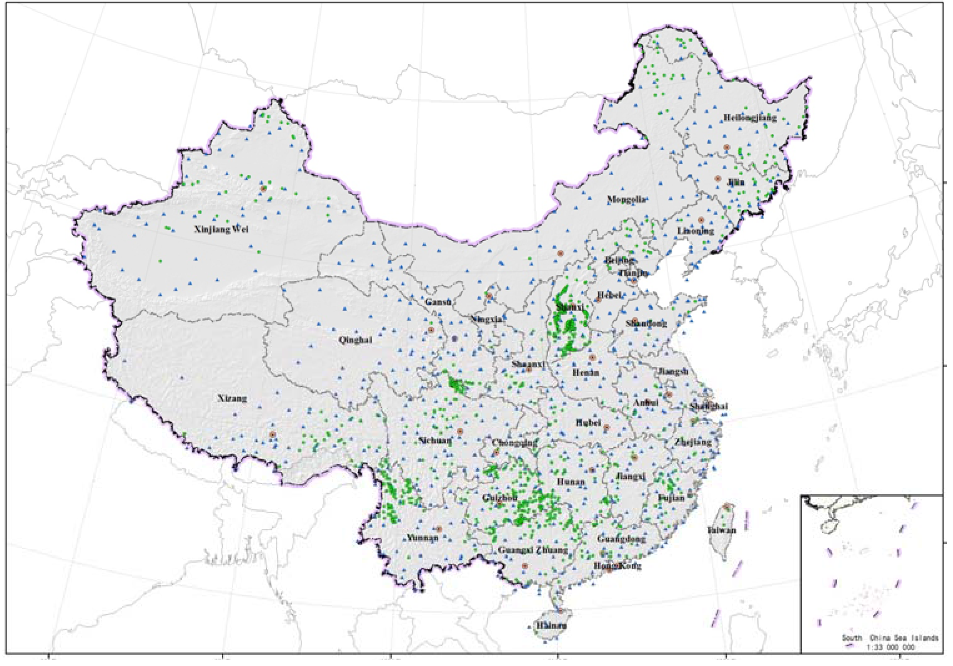Furthermore, the climatic variability, topographic complexity, and natural ecosystem diversity, as well as human disturbances, make China a large contributor to the global carbon cycle [14] (Figure 1).

2.1.2. Biomass Field Site Data

Biomass field site data was collected through vegetation from the China Ecosystem Research Network (CERN) from the site [32], which consisted of 1146 records (Figure 1), including forest, shrub, grass, and farmland. Moreover, all species of shrub and parts of herb layers are under forest communities. The survey data was collected in 2004, when the vegetation was at the accumulative process of the growth stage. The information including vegetation type, actual fresh and dry weight (including branch, limb, leaves, and roots), selected site and date, latitude, longitude, elevation, annual average temperature, and annual precipitation were recorded. According to land cover data, sample data can be divided into eight different biomass groups. The sample data was used for two methods: first, 90% of biomass sample data was used to established eight MLR models independently; second, 10% of sample data was applied to test simulation biomass value.

Figure 1. Location of the biomass estimation region. Blue triangles and inner green points represent weather stations and locations of biomass field sites, respectively.

Figure 1. Location of the biomass estimation region. Blue triangles and inner green points represent weather stations and locations of biomass field sites, respectively.

2.1.3. MODIS Data

The MODIS instrument is operating on both the Terra and Aqua spacecrafts. It has a viewing swath width of 2330 km and views the entire surface of the Earth every one-to-two days. Its detectors measure 36 spectral bands and it acquires data at three spatial resolutions: 250 m, 500 m, and 1000 m [33] MODIS vegetation index products have a wide range of applications, including global biogeochemical and hydrologic modeling, agricultural monitoring and forecasting, land-use planning, land cover characterization, and land cover change detection [34]. Normalized difference vegetation index (NDVI) and leaf area index (LAI) are important vegetation indices, widely applied in research on global, environmental, and climatic change. The MODIS/Terra 16-day L3 Global 250m NDVI product MOD13Q1 (d001–d353) and eight-day LAI product MOD15A2 (d001–d361) were obtained from the NASA website [35] in 2004 and 2010. However, noise induced by cloud contamination and atmospheric variability impeded the analysis and application of NDVI and LAI data. The most common criterion used to produce NDVI composite data is the maximum value composite (MVC) algorithm, which is applied to obtain a higher percentage of clear-sky data [34], and was also used to obtain LAI data.

The maximum value for the 19 NDVI and LAI images were extracted to reconstruct the NDVI-max and LAI-max during the study period, decreasing the outliers of the imagery. The NDVI-max and LAI-max are expressed as;

$$\text{NDVI max }=\text{ max }\left(\text{NDVIDOY}1\right)$$

(1)

$$\text{LAI max }=\text{ max }\left(\text{LAIDOY}2\right)$$

(2)

where DOY1 is from 1–353, and DOY2 is 1–361.

2.1.4. Other Datasets

Monthly mean temperature and precipitation for 756 standard weather stations were downloaded from the Chinese Central Meteorological Office in 2004 and 2010 as original textfile type. Firstly, the meteorological data was transformed to a point vector data-defined project and coordinate system at platform Arcgis 9.3. Secondly, the point data was interpolated to a 1 km × 1 km grid by kriging interpolation.

A digitized land cover, which consists of six vegetation types and 25 subtypes, was constructed from the vegetation map of China at 1:1,000,000 scale [36] in 2010. The vegetation classification on grid cells of 1 km × 1 km resolutions were extracted from the remote sensing images. Ten vegetation categories (Table 1) used herein were assigned from 25 subtypes. The vegetation data was used to overlay on multiple data extracting different types of biomass. The basic information, such as latitude, longitude, and elevation derived from Digital Elevation Model (DEM) data [37] was also re-sampled to a 1 km × 1 km resolution.

2.2. Methods

2.2.1. Model and Precision

MLR is a statistical tool that regresses independent variables against a dependent variable [38] In the context of this study, MLR is a supervised method that aims at establishing a mathematical relationship between a property of a given system and a set of molecular characteristics or descriptors that encode information, being expressed in Equation (3);

$$\text{Y}=\text{AX }+\text{ ε}$$

(3)

where ε is an n × 1 residuals vector; x is a known n × k matrix of description; A is a K × 1 vector of adjusted parameters; Y is a n × 1 vector of the response variable related with either the activity or other system property [39].

The model performance for MLR was assessed based on the agreements between the predicted value and the observed value. The agreements were quantified using relative estimation error (REE), which is calculated as Equation (4) [40]:

$$REE=\sqrt{\frac{{{\displaystyle \sum }}^{\text{}}{\left[\left({\text{Y}}_{\text{i}}-{\tilde{Y}}_{\text{i}}\right)/{\tilde{Y}}_{\text{i}}\right]}^2}{N}}$$

(4)

where Y_i is the observed data, ${\tilde{Y}}_{\text{i}}$ is the predicted value, and N is the number of validation points. Ninety percent of the biomass files were selected through a hierarchical sample method according to different classes for establishing regression models and the remainder 10% of samples were adopted to calculate REE.

MLR was calculated for the terrestrial ecosystem biomass of China in 2010. The simulation results were compared with the survey data, and the simulation precision was calculated using Equation (5) [41]:

$$Precision=1-\frac{V_{\text{m}}-V_{\text{s}}}{V_{\text{s}}}$$

(5)

where V_m is the value of simulated results by the regression model, and V_s is the value of survey data.

2.2.2. Variable Selection

The selected variables were considered as influence factors of several aspects, such as geographic elements (including longitude, latitude, and elevation) and environmental factors (including annual precipitation and annual averaged temperature) influencing the growth of vegetation, statistical data, and remote-sensing vegetation index (including NDVI and LAI), which directly showed the status of vegetation on a large scale. Geographic factors can be used as a reflection of different spatial distributions of biomass because of the position of vegetation growth. Environment factors reflect regional differences of biomass because of the sensitivity of vegetation on meteorological conditions. The changes in environmental conditions can determine shifts in the distribution of organisms [42]. Temperature and precipitation are essential factors for plant growth. Hydrothermal conditions have a significant impact on plant photosynthesis and biomass [43]. Temperature and precipitation are the dominant factors in controlling the distribution of vegetation carbon density [44].

The construction of MLR for biomass assessment was executed through a step-wise regression analysis using the eight predictive variables and the biomass variable. Different types have variable correlations. Finally, before variables can be considered, the correlation coefficients between biomass data and other factors must be tested. We divided them into eight groups according to different vegetation types. We have used the data analysis add-in, available in the software of SPSS, and different types have different correlations with different factors (Table 1). Farmland plants have a short growth period, and provide unsuitable continuous data to estimate, while there is a significant correlation between grain dry weight and biomass. The biomass density of desert and wetland was estimated as 20g m⁻² and 4000 g m⁻² [14].

Table 1. Correlation coefficients between dry weight and variation.

Variables	Forest					Shrub	Grass	Farmland
	EN	DC	EB	DB	MF
Elevation (E)	0.40 **		0.10	0.08
Latitude (LAT)	−0.18 **			−0.13 *		−0.46 **	−0.44 **
Longitude (LON)					−0.51 *
Annual Precipitation (Pre)	0.12 **			0.34 **
Annual Average Temperature (T)	−0.07		−0.10	0.19 **
LAI (LAI)	0.59 **	−0.59 **	−0.78 **	0.55 **	0.52*	0.22 *	0.38 **
NDVI (NDVI)		0.94 **		0.16 **
Grain dry weight (G)								0.87 **

Note: * represents p ≤ 0.05; ** represents p ≤ 0.01.

Table 1. Correlation coefficients between dry weight and variation.

Variables	Forest					Shrub	Grass	Farmland
	EN	DC	EB	DB	MF
Elevation (E)	0.40 **		0.10	0.08
Latitude (LAT)	−0.18 **			−0.13 *		−0.46 **	−0.44 **
Longitude (LON)					−0.51 *
Annual Precipitation (Pre)	0.12 **			0.34 **
Annual Average Temperature (T)	−0.07		−0.10	0.19 **
LAI (LAI)	0.59 **	−0.59 **	−0.78 **	0.55 **	0.52*	0.22 *	0.38 **
NDVI (NDVI)		0.94 **		0.16 **
Grain dry weight (G)								0.87 **

Note: * represents p ≤ 0.05; ** represents p ≤ 0.01.

2.2.3. Validation of the Results

Correlation analysis was conducted between biomass and eight factors. The linear relationships for the four primary types are given in Table 2. The R² value of DC forest was higher than other types, and grass had a lower R² value.

First, we obtained the biomass density of each type overlapping on land cover data, according to the model (Table 2), using a raster calculator module at the platform of Arcgis 9.3. Secondly, each grid had a biomass value, which was calculated as the biomass density multiplied by the area of each grid unit. Lastly, total biomass dry weight was spatially calculated in the whole region.

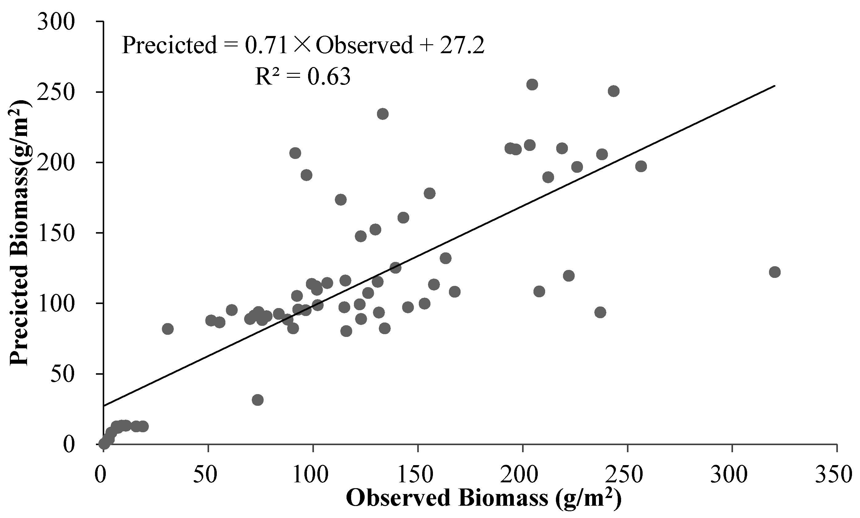
The results assured a good representation of the range of China’s ecosystem, and these observations were supported by MODIS data (NDVI, LAI), geographic elements (including longitude, latitude, and elevation), environmental factors (including annual precipitation and annual averaged temperature), and statistical data in the multiple regression model. More than 95% of the variance in ABGB density was explained, with a relative estimation error of 67 g·m⁻² for a range of biomass density in 2010 (Figure 2), when the residual data was used for training and cross-validation.

Table 2. Multiple linear regression model of 10 species.

Type	Linear relationship	R2	REE (%)
EN	Y1 = 0.097 E + 12.88 LAT + 0.07Pre + 18.14T + 14.35LAI + 779.38	0.52	32
DC	Y2 = 19.78LAI−49.14NDVI + 51.57	0.90	22
EB	Y3 = 0.061E + 6.51T + 16.17LAI − 119.55	0.74	24
DB	Y4 = 0.052E + 14.13LAT + 0.16Pre + 9.24T + 8.11LAI − 45.21NDVI − 686.68	0.49	9.4
MF	Y5 = −11.37LON + 12.03LAI + 1292.63	0.68	21
Shrub	Y6 = −0.59LAT + 0.15LAI + 21.94	0.27	1.5
Grass	Y7 = −0.20LAT + 0.09LAI + 6.76	0.36	0.38
Farmland	Y8 = 1.98G + 0.16	0.72	-
Wetland	Y9 = 400 g/m2	-	-
Desert	Y10 = 2 g/m2	-	-

Table 2. Multiple linear regression model of 10 species.

Type	Linear relationship	R2	REE (%)
EN	Y1 = 0.097 E + 12.88 LAT + 0.07Pre + 18.14T + 14.35LAI + 779.38	0.52	32
DC	Y2 = 19.78LAI−49.14NDVI + 51.57	0.90	22
EB	Y3 = 0.061E + 6.51T + 16.17LAI − 119.55	0.74	24
DB	Y4 = 0.052E + 14.13LAT + 0.16Pre + 9.24T + 8.11LAI − 45.21NDVI − 686.68	0.49	9.4
MF	Y5 = −11.37LON + 12.03LAI + 1292.63	0.68	21
Shrub	Y6 = −0.59LAT + 0.15LAI + 21.94	0.27	1.5
Grass	Y7 = −0.20LAT + 0.09LAI + 6.76	0.36	0.38
Farmland	Y8 = 1.98G + 0.16	0.72	-
Wetland	Y9 = 400 g/m2	-	-
Desert	Y10 = 2 g/m2	-	-

Figure 2. Relationship between observed biomass (g/m²) and multiple regression model predictions (g/m²).

Figure 2. Relationship between observed biomass (g/m²) and multiple regression model predictions (g/m²).

3. Results

3.1. Terrestrial Ecosystem Biomass

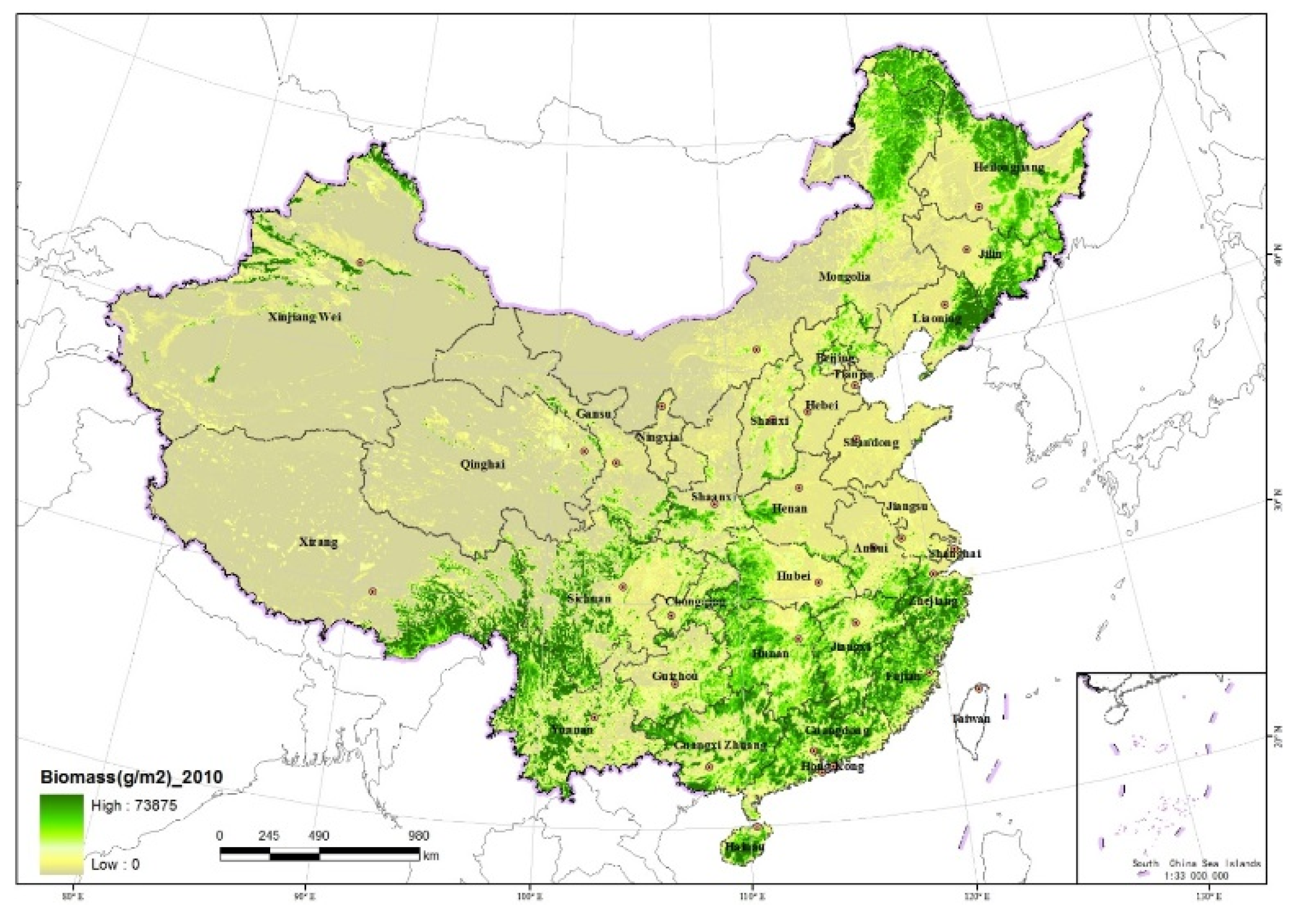
Before estimating biomass in 2010, according to the theory of geographic similitude phenomena, we had a hypothesis that the principles of biomass in 2010 would follow similar patterns as 2004. Thus, the same formula was used to estimate biomass in 2010. Using the multiple linear regression models, a continuous biomass density map of the terrestrial ecosystem of China was produced spatially in 2010 (Figure 3). The map shows the distribution of biomass across China varied from 0–73,875 g∙m⁻² in 2010 at 1 km spatial resolution. According to the map of forest age [45], most of high-value biomass is concentrated on old-age forest regions, such as the Great Canyon region of the Yalungzangbo River, southeast of the Qinghai-Tibetan Plateau and the Hengduan mountains; the Xing’an mountains in the autonomous region of Mongolia and the northeast regions; and the Changbai mountains in the northeast regions. As for the rich hydrothermal conditions, the plain and hilly regions in east and southeast China contained a relatively high total biomass value. The low biomass value is primarily distributed over the north and northwest regions, where desert areas are covered by few plants.

Table 3 shows biomass value related to land cover type classes, as provide by the land cover 2010 data. The result indicates that the biomass value of the entire ecosystem is 31.1 Pg in 2010. The average of vegetation is 3370 g m⁻². Our results show the non-uniform distribution of biomass storage in each land cover type. Forests are major contributors of terrestrial ecosystem biomass storage, which is estimated to have a value of 21.0 Pg for the year 2010, close to 70% of all biomass dry weight. Next is farmland, which has a 4.04 Pg biomass dry weight in 2010, accounting for around 13% of the whole ecosystem. The value of 3.32 Pg dry weight for grass, totaling 10.68% of all biomass in 2010, was estimated. The biomass of wetland is 1.37 Pg, accounting for 4.41% in 2010. The biomass dry weight of shrub is 0.98 Pg, 3.16% of total vegetation. Desert had the lowest biomass value in the terrestrial ecosystem, with only a 0.35 Pg share of biomass to 1.1% in 2010. The biomass density in the forest ecosystems were the largest when compared with other terrestrial ecosystems, while desert areas had the least in the whole ecosystem.

Table 3. Biomass of land cover type.

Type	Area (×104 km2)	Mean of Biomass (g/m2)	Total Biomass (Pg)	Percent of Biomass (%)
Forest	176.37	11912.6	21.01	67.61
Shrub	46.83	2098.1201	0.98	3.16
Grass	291.04	1139.15	3.32	10.68
Farmland	177.78	2274.68	4.04	13.00
Wetland	37.94	3602.59	1.37	4.41
Desert	191.92	183.22	0.35	1.13
All	921.87	3370.86	31.08	100.00

Table 3. Biomass of land cover type.

Type	Area (×104 km2)	Mean of Biomass (g/m2)	Total Biomass (Pg)	Percent of Biomass (%)
Forest	176.37	11912.6	21.01	67.61
Shrub	46.83	2098.1201	0.98	3.16
Grass	291.04	1139.15	3.32	10.68
Farmland	177.78	2274.68	4.04	13.00
Wetland	37.94	3602.59	1.37	4.41
Desert	191.92	183.22	0.35	1.13
All	921.87	3370.86	31.08	100.00

Figure 3. Distribution of ABGB density of China’s terrestrial ecosystem in 2010.

Figure 3. Distribution of ABGB density of China’s terrestrial ecosystem in 2010.

3.2. Province Biomass Distribution

Table 4 presents the studies and biomass statistical value of each province (not including Hong Kong, Macao, and Taiwan), including the average of biomass, total biomass, percent of biomass, and biomass per capita (calculated by permanent residents of each province). Biomass distribution differences exist in each province. Heilongjiang, Yunnan, and Mongolia occupied the top three largest regions for biomass storage, counting for more than 8% of China, while Shanghai and Tianjin had the least biomass storage among all provinces, with less than 0.1%. The three regions with the highest biomass density were Fujian, Zhejiang, and Hainan, which were all over 9000 g m⁻² in 2010, whereas the average biomass density was less than 1200 g m⁻² in Qinghai, Xinjiang and Ningxia.

Natural resources are the fundamental capital of human survival and development. Under the condition of a fixed capital, the greater the population, the fewer the units of output [46]. As the Chinese population grows, the consumption of natural resources increases. The per-capita natural resources of China are much lower than the global average. Biomass can reflect the storage of natural resources at a regional scale. Biomass per capita represents the reserve per individual. Table 4 displays the biomass of each province. To reflect actual conditions more accurately, the permanent population was calculated to biomass per capita. The results indicate that the province with the highest biomass per capita is Tibet, with a value of over 800 tons per individual according to the 2010 data. Shanghai and Tianjin, which are urban areas with a shortage of resources, have the lowest biomass per capita, as they contain areas with high population and limited space. Shanghai, Tianjin, Guangzhou, Beijing, and Hainan have negative growth of biomass per capita, indicating that these regions have fragile ecological carrying capacity.

Table 4. Biomass of terrestrial vegetation in each province of China in 2010.

Region	Mean Biomass (g/m2)	Total Biomass (Tg)	Percent of biomass (%)	Permanent population (ten thousand people)	Biomass per capita (Tons/pop)
Beijing	5197.66	82.10	0.26	1961	4.19
Tianjing	1960.99	21.70	0.07	1294	1.68
Hebei	2674.23	498.00	1.58	7185	6.93
Shanxi	2654.62	415.00	1.31	3571	11.62
Inner Mongolia	2305.08	2630.00	8.34	2471	106.52
Liaoning	5874.47	846.00	2.68	4375	19.33
Jilin	5398.2	1020.00	3.24	2746	37.28
Heilongjiang	6259.33	2810.00	8.91	3831	73.39
Shanghai	1967.85	11.20	0.04	2302	0.49
Jiangsu	2230.86	223.00	0.71	7866	2.83
Zhejiang	9594.76	959.00	3.04	5443	17.61
Anhui	3242.4	454.00	1.44	5950	7.64
Fujian	9791.05	1180.00	3.74	3689	31.97
Jiangxi	8112.91	1360.00	4.29	4457	30.41
Shandong	1802.9	274.00	0.87	9579	2.86
Henan	2548.59	421.00	1.34	9402	4.48
Hubei	5698.23	1060.00	3.36	5724	18.51
Hunan	7821.15	1660.00	5.25	6568	25.25
Guangdong	8768.96	1530.00	4.85	10,430	14.67
Guangxi	7579.01	1790.00	5.66	4603	38.83
Hainan	9577.15	322.00	1.02	867	37.10
Chongqing	4450.9	367.00	1.16	2885	12.71
Sichuan	5114.08	2480.00	7.87	8042	30.89
Guizhou	4325.91	761.00	2.41	3475	21.91
Yunnan	7155.36	2740.00	8.67	597	59.51
Xizang	2020.89	2420.00	7.68	300	807.21
Shaanxi	2696.75	554.00	1.76	733	14.87
Gansu	1201.45	511.00	1.62	2558	19.98
Qinghai	579.01	403.00	1.28	563	71.70
Ningxia	1163.57	60.40	0.19	630	9.59
Xinjiang	1044.07	1700.00	5.38	2181	77.88
Total	3351.098	31,600.00	100.00	126277	24.23

Table 4. Biomass of terrestrial vegetation in each province of China in 2010.

Region	Mean Biomass (g/m2)	Total Biomass (Tg)	Percent of biomass (%)	Permanent population (ten thousand people)	Biomass per capita (Tons/pop)
Beijing	5197.66	82.10	0.26	1961	4.19
Tianjing	1960.99	21.70	0.07	1294	1.68
Hebei	2674.23	498.00	1.58	7185	6.93
Shanxi	2654.62	415.00	1.31	3571	11.62
Inner Mongolia	2305.08	2630.00	8.34	2471	106.52
Liaoning	5874.47	846.00	2.68	4375	19.33
Jilin	5398.2	1020.00	3.24	2746	37.28
Heilongjiang	6259.33	2810.00	8.91	3831	73.39
Shanghai	1967.85	11.20	0.04	2302	0.49
Jiangsu	2230.86	223.00	0.71	7866	2.83
Zhejiang	9594.76	959.00	3.04	5443	17.61
Anhui	3242.4	454.00	1.44	5950	7.64
Fujian	9791.05	1180.00	3.74	3689	31.97
Jiangxi	8112.91	1360.00	4.29	4457	30.41
Shandong	1802.9	274.00	0.87	9579	2.86
Henan	2548.59	421.00	1.34	9402	4.48
Hubei	5698.23	1060.00	3.36	5724	18.51
Hunan	7821.15	1660.00	5.25	6568	25.25
Guangdong	8768.96	1530.00	4.85	10,430	14.67
Guangxi	7579.01	1790.00	5.66	4603	38.83
Hainan	9577.15	322.00	1.02	867	37.10
Chongqing	4450.9	367.00	1.16	2885	12.71
Sichuan	5114.08	2480.00	7.87	8042	30.89
Guizhou	4325.91	761.00	2.41	3475	21.91
Yunnan	7155.36	2740.00	8.67	597	59.51
Xizang	2020.89	2420.00	7.68	300	807.21
Shaanxi	2696.75	554.00	1.76	733	14.87
Gansu	1201.45	511.00	1.62	2558	19.98
Qinghai	579.01	403.00	1.28	563	71.70
Ningxia	1163.57	60.40	0.19	630	9.59
Xinjiang	1044.07	1700.00	5.38	2181	77.88
Total	3351.098	31,600.00	100.00	126277	24.23

4. Discussion

The results of terrestrial ecosystem biomass mapping demonstrate the utility of satellite data sets for estimating ABGB storage, even in the regions where, historically, researchers were unable to reach. The frequent temporal coverage of MODIS imagery increases the likelihood of capturing the continuous and timely information of plants, and the sensitivity of the composited reflectance of canopy density and structure provides the ability to link canopy reflectance to biomass. Vegetation growth can also be monitored by many other factors. We tested combinations of remote sensing data, including LAI and NDVI indices, as well as geographic elements (including longitude, latitude, and elevation) and environmental factors (including annual precipitation and annual average temperature). The statistical data, including grain dry weight, was added to these these variables to estimate the farmland biomass. As a result, according to the correlation between biomass sample data and these impact factors, we have established a multiple linear regression model and predicted the total biomass distribution of the terrestrial ecosystem of China in 2010.

We selected the estimates concerning the biomass storage and biomass density on different types of ecosystems (Table 5). Compared with other studies, we obtained the biomass value of the terrestrial ecosystem, including forest, grassland, and farmland biomass estimation, which was nearly consistent with previous data. While forest biomass is slightly larger than most former values, one reason to explain this is that the area larger. Shrub biomass is close to the data from former studies. Grass biomass is smaller than previous studies because of grass sample data where the grass under the forest has a lower biomass than separate grassland. Wetland and desert biomass is larger or smaller than previous data because we used the referenced biomass density value instead of the estimated one. Thus, the results of this study are reasonable.

Research gaps exist between this study and previous studies. There are several reasons that caused errors, with large uncertainties existing among the evaluations derived from various methods and data resources. The multiple linear regression models are strongly influenced by the distribution of the training data, and the selection of training data determines the precision of biomass estimation. Also, remotely sensed data combined with biomass sample data is mismatched between the area sampled on the ground and the resolution of the satellite imagery. Furthermore, many measures can also influence plant biomass. Since the mid-1970s, many management measures, such as reforestation and forest management, grassland protection, farming system reformation, and conservation tillage, have had an important role in carbon sequestration [44].

Table 5. Estimates on vegetation on the terrestrial ecosystem in China.

Vegetation type	Area (104 km2)	Biomass storage (Pg)	Biomass density (kg/m2)	References
Terrestrial ecosystem		13.09		[14]
		128.67		[47]
		78.29		[1]
		29.64		[48]
		31.20		[49]
		30.53		[50]
	899.04	30.47 ± 0.78		[44]
	921.87	31.1		Result of this paper
Forest		18.49		[44]
		12.24		[51]
	l18.45	20.23		[52]
		11.00		[53]
	149.12	10.67		[54]
		11.99		[55]
	176.37	21.01		Result of this paper
Shrub	154.63	3.73 ± 0.27	1.088 ± 0.077	[56]
	216.53	0.51	0.11	[48]
	207.6	2.12	0.60	[44]
	46.82	0.98	2.10	Result of this paper
Grassland	355.3	6.78	1.15	[25]
	331.4	2.56	0.35	[57]
	331	7.38	1.00	[20]
	334.1	2.33	0.31	[58]
	263.3	7.47	1.28	[48]
	331.4	6.04	0.82	[44]
	291	3.32	1.14	Result of this paper
Farmland	108	4.44		[44]
	177.78	4.04		Result of this paper
Wetland	11	0.53		[44]
	37.94	1.37		Result of this paper
Desert	128.24	1.04		[44]
	190	0.35		Result of this paper

Table 5. Estimates on vegetation on the terrestrial ecosystem in China.

Vegetation type	Area (104 km2)	Biomass storage (Pg)	Biomass density (kg/m2)	References
Terrestrial ecosystem		13.09		[14]
		128.67		[47]
		78.29		[1]
		29.64		[48]
		31.20		[49]
		30.53		[50]
	899.04	30.47 ± 0.78		[44]
	921.87	31.1		Result of this paper
Forest		18.49		[44]
		12.24		[51]
	l18.45	20.23		[52]
		11.00		[53]
	149.12	10.67		[54]
		11.99		[55]
	176.37	21.01		Result of this paper
Shrub	154.63	3.73 ± 0.27	1.088 ± 0.077	[56]
	216.53	0.51	0.11	[48]
	207.6	2.12	0.60	[44]
	46.82	0.98	2.10	Result of this paper
Grassland	355.3	6.78	1.15	[25]
	331.4	2.56	0.35	[57]
	331	7.38	1.00	[20]
	334.1	2.33	0.31	[58]
	263.3	7.47	1.28	[48]
	331.4	6.04	0.82	[44]
	291	3.32	1.14	Result of this paper
Farmland	108	4.44		[44]
	177.78	4.04		Result of this paper
Wetland	11	0.53		[44]
	37.94	1.37		Result of this paper
Desert	128.24	1.04		[44]
	190	0.35		Result of this paper

5. Conclusions

Although there are many studies on biomass estimation, few have estimated the ABGB of the whole terrestrial ecosystem spatially and over time. The remote sensing indices were one of the primary factors of vegetation monitoring. Temperature and precipitation are the dominant factors in controlling the distribution of vegetation carbon density [44]. According to the results, we can obtain the following conclusions.

Firstly, the biomass vary differently in spatial distribution: the high values occurred in the Great Canyon region of Yalungzangbo River, southeast of the Qinghai-Tibetan Plateau and the Hengduan Mountains; the Xing’an mountains in the autonomous region of Mongolia and the northeast regions; the Changbai mountains in the northeast regions; and the plain and hilly regions in east and southeast China. The low biomass values were primarily distributed in north and northwest regions, where it is mostly desert with few plants.

Secondly, the ABGB of China was estimated to be 31.1 Pg (1 Pg = 1015 g) in 2010. The forest ecosystem contains the largest total biomass, which represents about 70% of the whole terrestrial ecosystem. Desert had the least biomass value in the terrestrial ecosystem, with only 0.35Pg share of biomass to 1.1% in 2010. The biomass density in the forest ecosystem is also larger when compared with other terrestrial ecosystems, while desert is the smallest in the entire ecosystem.

Lastly, higher biomass densities are usually found in the mountain areas, where vegetation is dense. Lower biomass densities are usually found in the desert areas, where there is no vegetation or it is sparse. Western and northwest areas with wealth of natural resources and sparse population, has the larger biomass per capita with 807 t in 2010. However, eastern and coastal areas with high population densities and minimal space, has only less than 0.5 t biomass per individual.

Lastly, biomass distribution differences exist in all provinces. The regions of Heilongjiang, Yunnan, and Mongolia occupied the top three largest biomass storage areas, more than 8% of China, while Shanghai and Tianjin were the smallest among all provinces, with less than 0.1% of the country’s biomass storage. The three highest biomass densities are found in Fujian, Zhejiang, and Hainan, which are all over 9000 g∙m⁻², whereas the average biomass is less than 1200 g∙ m⁻² in Qinghai, Xinjiang and Ningxia. Tibet, with a wealth of natural resources and sparse population, has the largest biomass per capita with 807t in 2010. Shanghai and Tianjin, with high population densities and minimal space, had only less than 0.5t biomass per individual. For Shanghai, Tianjin, Guangzhou, Beijing, and Hainan, with negative growth of biomass per capita, the data clearly indicates that these regions with fragile ecological carrying capacity.

Biomass maps can be used as baseline information for future landscape level studies, such as greenhouse gas inventories and terrestrial carbon accounting, or for monitoring management practices. As the development of the economy of China intensifies, the demand for new fuel energy will put significant pressure on existing natural resources. Reliable and current information on the spatial distribution of the terrestrial ecosystem biomass of China is required. However, because of the limitations of data acquisitionm we just use one year of data to estimate the biomass models. Actually, there is a risk and defect to data inversion. We plan to collect data from more years to perfect this data in our further research.

References

- Ni, J. Carbon storage in terrestrial ecosystems of China: Estimates at different spatial resolutions and their responses to climate change. Clim. Change 2001, 49, 339–358. [Google Scholar] [CrossRef]
- Schlesinger, W.H. Carbon balance in terrestrial detritus. Ann. Rev. Ecol. Syst. 1977, 8, 51–81. [Google Scholar] [CrossRef]
- Cao, M.; Woodward, F.I. Net primary and ecosystem production and carbon stocks of terrestrial ecosystems and their responses to climate change. Global Change Biol. 1998, 4, 185–198. [Google Scholar] [CrossRef]
- Myneni, R.B.; Keeling, C.J.; Asrar, G.; Nemani, R.R. Increased plant growth in the northern high latitudes from 1981 to 1991. Nature 1997, 386, 698–702. [Google Scholar] [CrossRef]
- Turner, D.P.; Ritts, W.D.; Cohen, W.B.; Maeirsperger, T.K.; Gower, S.T.; Kirschbaum, A.A.; Running, S.W.; Zhao, M.; Wofsy, S.C.; Dunn, A.L. Site-level evaluation of satellite-based global terrestrial gross primary production and net primary production monitoring. Global Change Biol. 2005, 11, 666–684. [Google Scholar] [CrossRef]
- Zolkos, S.G.; Goetz, S.J.; Dubayah, R.A. meta-analysis of terrestrial aboveground biomass estimation using lidar remote sensing. Remote Sens. Environ. 2013, 128, 289–298. [Google Scholar] [CrossRef]
- Tan, K.; Piao, S.; Peng, C.; Fang, J. Satellite-based estimation of biomass carbon stocks for northeast China’s forests between 1982 and 1999. Forest Ecol. Mang. 2007, 240, 114–211. [Google Scholar] [CrossRef]
- Caccamo, G.; Chisholm, L.A.; Bradstock, R.A.; Puotinen, M. Assessing the sensitivity of MODIS to monitor drought in high biomass ecosystems. Remote Sens. Environ. 2011, 115, 2626–2639. [Google Scholar] [CrossRef]
- Le Maire, G.; Marsden, C.; Nouvellon, Y.; Grinand, C.; Hakamada, R.; Stape, J.L.; Laclau, J. MODIS NDVI time-series allow the monitoring of Eucalyptus plantation biomas. Remote Sens. Environ. 2011, 115, 2613–2625. [Google Scholar] [CrossRef]
- Houghton, R.A.; Butman, D.; Bunn, A.G.; Krankina, O.N.; Schlesinger, P.; Stone, T.A. Mapping Russian forest biomass with data from satellites and forest inventories. Environ. Res. Lett. 2007, 2, 1–7. [Google Scholar] [CrossRef]
- Lu, D. The potential and challenge of remote sensing-based biomass estimation. Int. J. Remote Sens. 2006, 27, 1297–1328. [Google Scholar] [CrossRef]
- Houghton, R.A.; Hall, F.; Goetz, S.J. Importance of biomass in the global carbon cycle. J. Geophys. Res. 2009, 114, 1–13. [Google Scholar] [CrossRef]
- Goetz, S.J.; Baccini, A.; Laporte, N.T.; Johns, T.; Walker, W.; Kellndorfer, J.; Houghton, R.A.; Sun, M. Mapping & monitoring carbon stocks with satellite observations: A comparison of methods. Carbon Bal. Manage 2009, 4, 1–7. [Google Scholar]
- Fang, J.Y.; Liu, G.; Xu, S. Carbon cycle of terrestrial ecosystems in China and its global significance. In Hot Spots in Modern Ecolog; Wang, R.S., Fang, J.Y., Gao, L., Feng, Z.W., Eds.; Science and Technology Press: Beijing, China, 1996; pp. 240–250. [Google Scholar]
- Huang, G.S.; Xiao, C.Z. MODIS-based estimation of forest biomass in Northeast China. Forest Res. Manag. 2005, 4, 40–44. [Google Scholar]
- Guo, Z.; Hu, H.; Li, P.; Li, N.; Fang, J. Spatio-temporal changes in biomass carbon sinks in China’s forests from 1977 to 2008. Sci. China Life Sci. 2013, 56, 661–671. [Google Scholar] [CrossRef] [PubMed]
- Wang, X.; Fang, J.; Zhu, B. Forest biomass and root–shoot allocation in northeast China. Forest Ecol. Manag. 2008, 225, 4007–4020. [Google Scholar] [CrossRef]
- Xu, B.; Guo, Z.; Piao, S.; Fang, J. Biomass carbon stocks in China’s forests between 2000 and 2050: A prediction based on forest biomass–age relationships. Sci. China Life Sci. 2012, 53, 776–783. [Google Scholar] [CrossRef] [PubMed]
- Guo, Q.; Hu, Z.; Li, S.; Li, X.; Sun, X.; Yu, G.; Hu, Z.; Li, S.; Li, X.; Sun, X.; et al. Spatial variations in aboveground net primary productivity along a climate gradient in Eurasian temperate grassland: effects of mean annual precipitation and its seasonal distribution. Global Change Biol. 2012, 18, 3624–3631. [Google Scholar] [CrossRef]
- Fan, J.; Zhou, H.; Harris, W.; Yu, G.; Wang, S.; Hu, Z.; Yue, Y. Carbon storage in the grasslands of China based on field measurements of above- and below-ground biomass. Clim. Change 2008, 86, 375–396. [Google Scholar] [CrossRef]
- Piao, S.L.; Fang, J.; He, J.S.; Xiao, Y. Spatial Distribution of Grassland Biomass in China. Acta Phytoecol. Sin. 2004, 28, 491–498. [Google Scholar]
- Wang, L.; Niu, K.; Yang, Y.; Zhou, P. Patterns of above- and belowground biomass allocation in China’s grasslands: Evidence from individual-level observations. Sci. China Life Sci. 2010, 537, 851–857. [Google Scholar] [CrossRef] [PubMed]
- Ma, A. Introduction to Geographic Science “Bridge Science” Between Natural Science and Social Science; Higher Education Press: Beijing, China, 2005; pp. 9–104, 137–147. [Google Scholar]
- Tong, H. Methods of Modeling Forest Biomass Based on Remote Sensing Information; Beijing Forestry University: Beijing, China, 2007. [Google Scholar]
- Ni, J. Carbon storage in grasslands of China. J. Arid Environ. 2002, 50, 205–218. [Google Scholar] [CrossRef]
- Zhang, J.C. Climate of China; China Meteorology Press: Beijing, China, 1991. [Google Scholar]
- Yu, G.; Chen, Z.; Piao, S.; Peng, C.; Ciais, P.; Wang, Q.; Li, X.; Zhu, X. High carbon dioxide uptake by subtropical forest ecosystems in the East Asian monsoon region. Pro. Natl. Acad. Sci. USA 2014, 111, 4910–4915. [Google Scholar] [CrossRef] [PubMed]
- Piao, S.; Fang, J.; Ciais, P.; Peylin, P.; Huang, Y.; Sitch, S.; Wang, T. The carbon balance of terrestrial ecosystems in China. Nature 2009, 458, 1009–1013. [Google Scholar] [CrossRef] [PubMed]
- Ministry of Forestry of China. Forest Resource Report of China-the 7th National Forest Resources Inventory; China Forestry Publishing House: Beijing, China, 2009.
- China forestry sustainable development strategy research group. General View of China Forestry Sustainable Development Strategy Research. Beijing; China Forestry Publishing House: Beijing, China, 2002.
- Bai, Y.; Huang, J.; Zhen, S.; Pan, Q.; Zhang, L.; Zhou, H.; Xu, H.; Li, Y.; Ma, J. Drivers and regulating mechanisms of grassland and desert ecosystem services. Chinese J. Plant Ecol. 2014, 38, 93–102. [Google Scholar]
- China Ecosystem Research Network (CERN). Available online: http://www.cerndata.ac.cn/ (accessed on 22 June 2015).
- Moderate Resolution Imaging Spectroradiometer (MODIS). Available online: https://lpdaac.usgs.gov/products/modis_products_table/modis_overview#sthash.FEmodOUq.dpuf (accessed on 20 May 2015).
- Gu, J.; Li, X.; Huanga, C.; Okin, G.S. A simplified data assimilation method for reconstructing time-series MODIS NDVI data. Adv. Space Res. 2009, 44, 501–509. [Google Scholar] [CrossRef]
- LAI product MOD15A2 (d001–d361). Available online: ftp:e4ft01.cr.usgs.gov/ (accessed on 16 June 2015).
- Zhang, Z.; Wang, C.; Wang, F.; Wen, Q.; Zuo, L.; Dong, T.; Zhou, W.; Zhang, S; Wu, S.; Yan, C.; et al. Remote Sensing Monitoring of Landcover in China; Planet Map Publishing House: Beijing, China, 2010; pp. 7–8. [Google Scholar]
- Digital Elevation Model (DEM) data. Available online: http://www.csdb.cn/ (accessed on 13 June 2015).
- Darnag, R.; Minaoui, B.; Fakir, M. QSAR models for prediction study of HIV protease inhibitors using support vector machines, neural networks and multiple linear regression. Arab. J. Chem. 2012, 10, 1–32. [Google Scholar] [CrossRef]
- Ventura, C.; Latino, D.; Martins, F. Comparison of multiple linear regressions and neural networks based QSAR models for the design of new antitubercular compounds. Eur. J. Med. Chem. 2013, 70, 831–845. [Google Scholar] [CrossRef] [PubMed]
- Xu, B.; Yang, X.; Tao, W.; Qin, Z.; Liu, H.; Miao, J. Remote sensing monitoring upon the grass production in China. Acta Ecol. Sin. 2007, 27, 405–413. [Google Scholar] [CrossRef]
- Fu, X.; Tang, C.; Zhang, X.; Fu, J.; Jiang, D. An improved indicator of simulated grassland production based on MODIS NDVI and GPP data: A case study in the Sichuan province, China. Ecol. Indic. 2014, 40, 102–108. [Google Scholar] [CrossRef]
- Gómez-Bolea, A.; Llop, E.; Ariño, X.; Saiz-Jimenez, C.; Bonazza, A.; Messina, P.; Sabbioni, C. Mapping the impact of climate change on biomass accumulation on stone. J. Cult. Herit. 2012, 13, 254–258. [Google Scholar] [CrossRef]
- Huang, F.; Gao, Q.; Fu, D.; Liu, Z. Relation between climate variables and the aboveground biomass of Thymus mongolicus-Stipa bungeana community in steppe of Ordos Plateau, Inner Mongolia. Acta Ecol. Sin. 2001, 20, 1339–1346. [Google Scholar]
- Yu, G.; Li, X.; Wang, Q.; Li, S. Carbon storage and its spatial pattern of terrestrial ecosystem in China. J. Resour. Ecol. 2010, 2, 97–109. [Google Scholar]
- Wang, S.; Chen, J.M.; Ju, W.M.; Feng, X.; Chen, M.; Chen, P.; Yu, G. Carbon sinks and sources in China’s forests during 1901–2001. J. Environ. Manage. 2007, 85, 524–537. [Google Scholar] [CrossRef] [PubMed]
- Solow, R.M. A Contribution to the Theory of Economic Growth. Q. J. Econ. 1956, 70, 65–94. [Google Scholar] [CrossRef]
- Peng, C.H.; Apps, M.J. Contribution of China to the global carbon cycle since the last glacial maximum. Tellus 1997, 49, 393–408. [Google Scholar] [CrossRef]
- Kerang, L.; Wang, S.; Cao, M. Vegetation and soil carbon storage in China. Sci. China Earth Sci. 2004, 47, 49–57. [Google Scholar]
- Huang, M.; Ji, J.J.; Cao, M.K.; Li, K.R. Modeling study of vegetation shoot and root biomass in China. Acta Ecol. Sin. 2006, 26, 4156–4163. [Google Scholar]
- Ji, J.; Huang, M.; Li, K. Prediction of carbon exchanges between China terrestrial ecosystem and atmosphere in 21st century. Sci. China Earth Sci. 2008, 51, 885–898. [Google Scholar] [CrossRef]
- Xu, X. Impact of afforestation on carbon storage of forest ecosystem. Ph.D. Thesis, University of Chinese Academy of Sciences, Beijing, China, 2006. [Google Scholar]
- Fang, J.; Liu, G.; Xu, S. Biomass and net production if forest vegetaion in China. Acta Ecol. Sin. 1996, 16, 497–508. [Google Scholar]
- Liu, S.; Zhou, T.; Shu, Y.; Dai, M.; Wei, L.; Zhang, X. The estimating of the spatial distribution of forest biomass in China based on remote sensing and downscaling techniques. Acta Ecol. Sin. 2012, 32, 2320–2330. [Google Scholar]
- Xiao, X. Study on forest biomass and productivity in China. Ph.D. Thesis, Northeast Forestry University, Ha’erbin, China, 2005. [Google Scholar]
- Food and Agriculture Organization of the United Nations. Global Forest Resources Assessments (FRA). Available online: http://www.fao.org/forestry/fra/en/ (accessed on 16 May 2015).
- Hu, H.; Wang, Z.; Liu, G.; Fu, B. Vegetation carbon storage of major shrublands in China. Acta Phytoecol. Sin. 2006, 30, 539–544. [Google Scholar]
- Fang, J.; Guo, Z.; Piao, S.; Chen, A. Terrestrial vegetation carbon sinks in China, 1981–2000. Sci. China Earth Sci. 2007, 50, 1341–1350. [Google Scholar] [CrossRef]
- Piao, S.; Fang, J.; Zhou, L.; Tan, K.; Tao, S. Changes in biomass carbon stocks in China’s grasslands between 1982 and 1999. Global Biogeochem. Cycles 2007. [Google Scholar] [CrossRef]
© 2015 by the authors; licensee MDPI, Basel, Switzerland. This article is an open access article distributed under the terms and conditions of the Creative Commons Attribution license (http://creativecommons.org/licenses/by/4.0/).