The Impact of Local Microclimate Boundary Conditions on Building Energy Performance

Abstract

Local environmental boundaries play an important role in determining microclimate conditions affecting thermal-energy behavior of buildings. In this scenario, the purpose of the present work is to investigate how residential buildings are affected by different local microclimate conditions. To this aim, the continuous microclimate monitoring of (i) a rural area; (ii) a suburban area; and (iii) an urban area is carried out, and the comparative analysis of the different boundary conditions is performed. In particular, the effect of the presence of a large lake in the rural area on building energy demand for heating and cooling is evaluated, both in winter and summer. Coupled degree hour method and numerical analysis are performed in order to predict the energy requirement of buildings subject to local microclimate boundary conditions. The main results show higher air temperature and relative humidity values for the rural area. No significant mitigation effect due to the lake presence is found in urban and suburban areas because of the peculiar wind regime of the region. Additionally, the dynamic thermal-energy simulation shows a decrease of 14% and 25% in the heating consumption and an increase of 58% and 194% in cooling requirements of buildings situated in the rural area around the lake compared to the urban and suburban areas, respectively.

1. Introduction

Recently, climate change [1,2] has become a fundamental research issue, given the problems caused by such phenomena both at local and global scale. Meteorologists and climatologists studied climate variability on weekly [3] and annual or inter-annual scale, respectively, in order to provide reliable data to be used by designers and urban planners in the design of more adaptable and resilient buildings [4,5].

In general, the local climate conditions characterizing an area depend on many factors such as topography, altitude, morphology, presence of vegetation [6,7], orientation, urbanization level, etc. [8]. Additionally, the presence of huge masses of water such as lakes can significantly influence the surrounding environment and its local microclimate [9], by mitigating the ambient air temperature. Lakes are able to mitigate the microclimate of their surroundings by cooling and heating the local atmosphere during the day and night in summer and winter, respectively.

The capability of lakes to reduce daily and seasonal temperature fluctuation depends on the size of the lake itself and on its surface/volume ratio. In this scenario, field measurements of air temperature, relative humidity, black globe temperature, and wind speed were performed in Guangzhou, China [10], in order to define the effects of the presence of the lake, shade trees, and ground surface character on the microclimate. The capability of lakes to perturb local climate conditions through mesoscale circulation was demonstrated in [11], through numerical simulations of atmosphere-lake interactions in northern Canada. While the effects of climate change on lakes’ ecosystems [12] and of other local climate phenomena, e.g., urban heat island, on building thermal-energy performance are already investigated and well documented [13], a lack of knowledge about the impact of the lake’s presence on the local microclimate and on the surrounding buildings’ energy need is detected [14]. Nevertheless, the role of local microclimate variations generated by huge masses of water in affecting buildings energy requirement represents an important issue, given that buildings are responsible for ~40% of global energy consumption in developed countries [15,16].

Many studies focused on the impact of climate change phenomena, such as global warming and urban heat island phenomena, on the thermal-energy performance of buildings [17,18] and on the reduction of these phenomena [19]. These phenomena generate the increase of the ambient temperature in urban areas by modifying local microclimate [20,21] and consequently building energy consumption. Increased urban temperatures, modified radiation balance, different wind speeds, and altered solar gains have a huge impact on building energy production and consumption [22,23]. For this reason, the use of commonly available typical weather data sets for predicting buildings’ energy demand through numerical analysis, such as the widely used Typical Meteorological Year (TMY2) [24], the International Weather for Energy Calculation (IWEC) or the Test Reference Year (TRY), could leads to misleading decision-making process in quantifying energy efficiency in buildings located in different areas [25]. This is due to the fact that such weather files do not take into account local micro-climate phenomena, i.e., the long-term weather conditions, to which buildings belonging to a small and specific area within a larger area are subjected. For this reason, it is important to monitor local microclimate variation and phenomena, in terms of local environmental parameters, in order to provide representative and local weather data for accurately predicting building energy demand.

Many researchers use the degree day or degree hour method to estimate the impact of climate change on building’s energy demand [26]. Such method is useful to estimate the building energy requirement for heating and cooling based on human comfort levels and available meteorological temperature records for a given area and timeframe [27,28]. It requires a relatively long series of daily/hourly data from weather stations, and is typically used for studying the environmental parameters’ distribution with varying urban environment [29]. Additionally, whole-building dynamic simulation tools represent a good method to estimate building energy performance variations in different boundary conditions usually neglecting local envelope phenomena such as thermal bridges [30,31]. It allows simulating the energy flows related to the building energy requirements through simple input data related to (i) building features [32] and (ii) weather data sets.

From a deep literature review, it is evident that the effects of climate change and local climate phenomena in urban environment are widely investigated, especially in terms of building energy consumption. However, a lack of scientific research is still detected about the impact of local microclimate phenomena on building thermal-energy performance.

The purpose of the present work is to bridge such gap by investigating the variability of local climate due to different environmental boundaries. To this aim, the continuous microclimate monitoring of (i) a rural area; (ii) a suburban area; and (iii) an urban area of the same temperate climate zone is carried out. In particular, the microclimate generated by the presence of Lake Trasimeno (central Italy) in the rural area is investigated. Additionally, the impact of local climate variability on buildings’ energy demand is investigated in terms of heating and cooling requirement, through coupled degree hour method and numerical analysis. The present work aims to quantify the local microclimate differences and their effect on building behavior.

The final aim is to demonstrate whether or not it is necessary to provide tailored weather data sets [33] representative of the real and local microclimate while predicting building energy performance, even in those areas where urban development does not stress out the local environment very much like in central Italy.

2. Method and Measurement

The in-field continuous monitoring of the microclimate of (i) a rural; (ii) a suburban; and (iii) an urban area in central Italy was simultaneously carried out during winter and summer 2014, in order to quantify the local climate variation generated by different environmental boundaries. In particular, the microclimate local effects of a large lake, i.e., Lake Trasimeno (central Italy), were assessed, by recording weather data in its proximity and comparing such data with readings from the suburban and the urban location.

The degree hour method was applied in order to estimate the influence of such microclimate variability on building energy demand. Additionally, the energy requirement of a reference residential building was evaluated in the three different local microclimate scenarios, i.e., rural, suburban, and urban microclimate, through dynamic simulation. In particular, the analysis focused on the comparison between the rural area, characterized by the close proximity of Lake Trasimeno, and the other two investigated areas, i.e., suburban and urban areas. The considered urban area is represented by a middle-size town in central Italy (Perugia) where the urban development has to be considered relatively well mitigated with respect to sprawled dense cities.

The aim was to highlight how local microclimate boundary conditions are able to modify surrounding buildings’ energy requirements for heating and cooling.

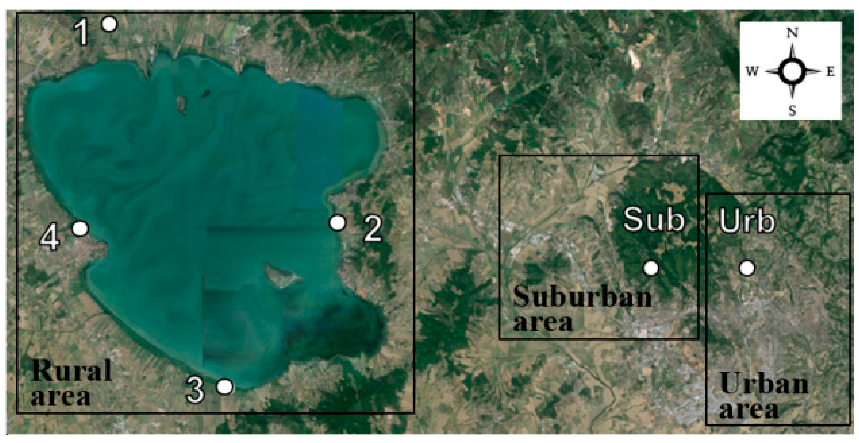
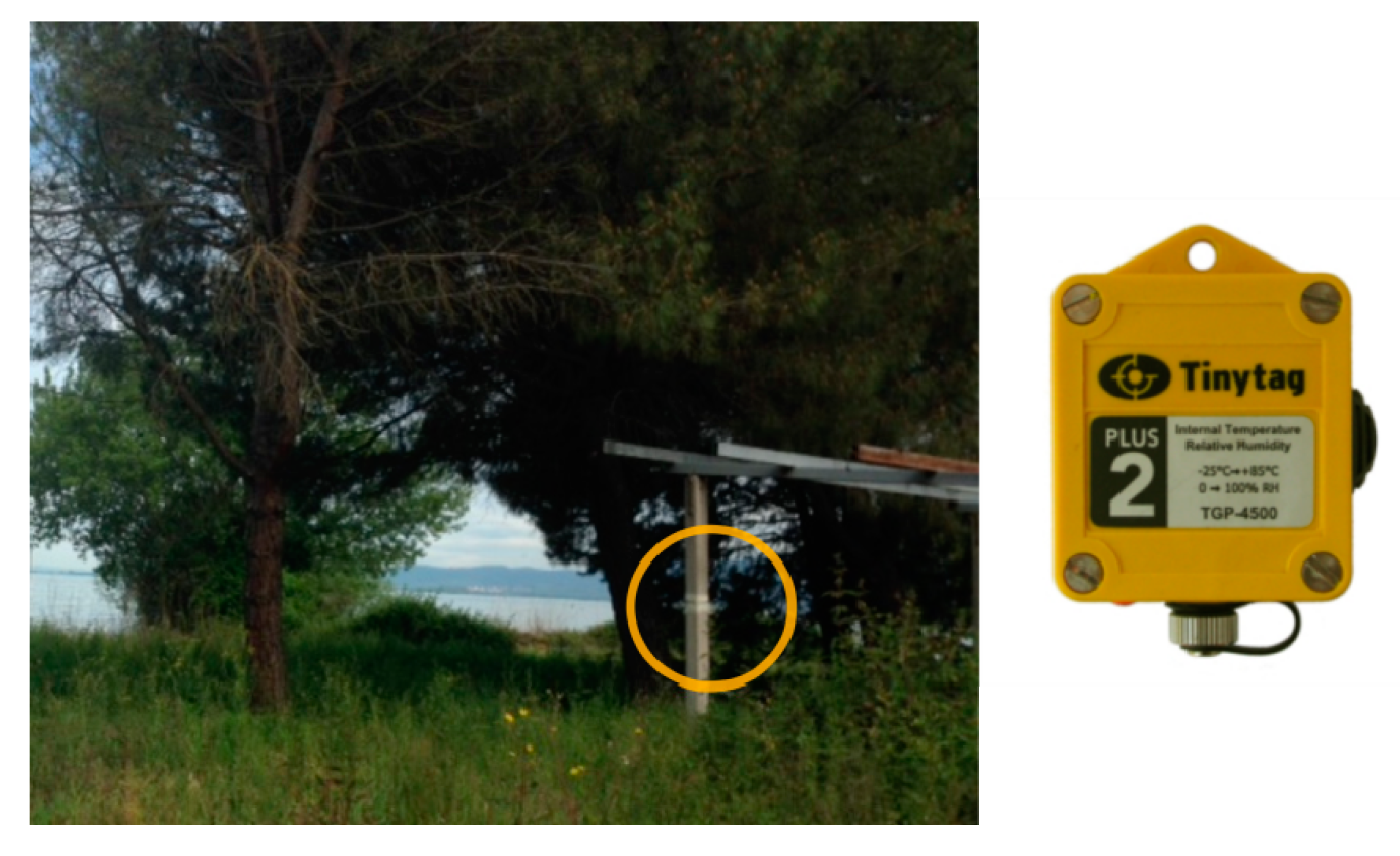
2.1. Microclimatic and Meteorological Monitoring

An in-field monitoring campaign was carried out during winter (January–April) and summer (July–August) 2014.

Figure 1 shows Lake Trasimeno Basin with the spatial distribution of four environmental sensors (1, 2, 3, and 4) positioned in the rural area, and of two meteorological stations located in the suburban (Sub) and urban area (Urb), respectively.

Figure 1. Aerial view of Lake Trasimeno basin. Spatial distribution of the hygrothermal sensors (1, 2, 3, and 4) and of the meteorological stations (Sub and Urb).

Figure 1. Aerial view of Lake Trasimeno basin. Spatial distribution of the hygrothermal sensors (1, 2, 3, and 4) and of the meteorological stations (Sub and Urb).

The sensors 1, 2, 3, and 4 are equal and were used to measure ambient dry bulb air temperature (T) and air relative humidity (RH) in four measurement spots close to Lake Trasimeno. In particular, the hygrothermal sensors were positioned in correspondence of the first line of the buildings in front of the lake, at an average distance of 400 m from the lakeshore (see Figure 2). Each sensor is able to measure temperatures between −25 °C and +85 °C, and relative humidity values between 0% and 100%. The measurement frequency was set every 10 min, and then hourly values were calculated during the post-processing of the data.

A detailed description of the measurement spots selected in the proximity of the lakeshore according to the cardinal points is provided in Table 1.

Given the configuration of the existing buildings around the lake, the sensors located in the measurement spots 1 and 4 were positioned on the terrace of the 1st floor of low-height buildings, at a height of 4 m above the ground level, while sensors located in measurement spots 2 and 3 were installed on the column of the crumbling structures of one floor buildings, at a height of 2 m (see Figure 2). The north-facing sensors were shaded from solar radiation by means of ventilated white boxes in order to achieve comparable measurement conditions. Additionally, the meteorological data of two complete dedicated weather stations (Figure 3) situated on the East side of Lake Trasimeno in a suburban (Sub) and an urban (Urb) area, respectively, were used for comparative purpose. Such weather stations are able to measure and collect air temperature, air relative humidity, global and direct solar radiation, wind speed and direction every 10 min through a dedicated measurement and data-logging apparatus. Therefore, hourly values were calculated and used during the data analysis.

Details about the location of the two weather stations are provided in Table 2.

Figure 2. Example of a measurement spot close to Lake Trasimeno (measurement spot no. 2) and hygrothermal sensor.

Figure 2. Example of a measurement spot close to Lake Trasimeno (measurement spot no. 2) and hygrothermal sensor.

Table 1. Description of the measurement spots close to Lake Trasimeno.

Measurement Spot no.	Village Name	Relative Position to the Lake	Vegetation Presence	Altitude [m a.s.l.]	Height * [m]
1	Tuoro	North	moderate	267	4
2	Torricella	East	rich	258	2
3	Mirabella	South	moderate	258	2
4	Castiglione del Lago	West	moderate	259	4

* Height over the ground level.

Table 1. Description of the measurement spots close to Lake Trasimeno.

Measurement Spot no.	Village Name	Relative Position to the Lake	Vegetation Presence	Altitude [m a.s.l.]	Height * [m]
1	Tuoro	North	moderate	267	4
2	Torricella	East	rich	258	2
3	Mirabella	South	moderate	258	2
4	Castiglione del Lago	West	moderate	259	4

* Height over the ground level.

Figure 3. (a) Urban and (b) suburban weather station.

Figure 3. (a) Urban and (b) suburban weather station.

Table 2. Description of the suburban and urban meteorological stations’ area.

Meteorological Station no.	Location Name	Distance to the Lake [km]	Level of Urbanization	Vegetation Presence	Altitude [m a.s.l.]	Height * [m]
Sub	Corciano	16.5	low	plentiful	520	2.5
Urb	Perugia	20.3	average	moderate	320	2.5

* Height over the plan of construction.

Table 2. Description of the suburban and urban meteorological stations’ area.

Meteorological Station no.	Location Name	Distance to the Lake [km]	Level of Urbanization	Vegetation Presence	Altitude [m a.s.l.]	Height * [m]
Sub	Corciano	16.5	low	plentiful	520	2.5
Urb	Perugia	20.3	average	moderate	320	2.5

* Height over the plan of construction.

2.2. Analysis of Building Energy Requirement with Varying Weather Conditions

The degree hour method [34,35] was chosen for the comparative prediction of buildings’ energy demand for heating and cooling in the rural, suburban, and urban area. This steady-state method is based on the fact that the amount of energy needed to heat or cool buildings located in different areas is directly proportional to the number of heating or cooling degree hours experimentally measured in those same areas during the summer and winter monitored period. Therefore, the quantitative estimation of the energy required for the buildings located in the three case study areas was carried out starting from the air temperature values measured in each area.

The heating degree hour index (HDH) and the cooling degree hour index (CDH) are calculated as the difference of mean hourly temperature with respect to a reference temperature according to the following Equations (1) and (2):

$$HDH=1h\cdot {\displaystyle \sum _{i=1}^{n}HD{H}_i}=1h\cdot {\displaystyle \sum _{i=1}^n\left(\text{max}\left(T_r-T_i,0\right)\right)[\text{h°C}]}$$

(1)

$$CDH=1h\cdot {\displaystyle \sum _{i=1}^{n}CD{H}_i}=1h\cdot {\displaystyle \sum _{i=1}^n\left(\max \left(T_i-T_r,0\right)\right)[\text{h°C}]}$$

(2)

These indexes depend on the number of hours considered for the calculation (n), the outdoor air temperature (T_i), and the reference temperature (T_r), representing the outdoor temperature below/above which the heating/cooling system is turned on. In the Mediterranean area, the reference temperature corresponds to 15 °C and 25 °C, for winter and summer, respectively, according to [36]. These values were chosen in order to keep indoor comfort conditions according to ASHRAE 2011 [37], and minimum energy consumption.

2.3. Energy Dynamic Simulation Modeling of the Case Study Building

The dynamic simulation for a reference residential building was carried out in three different scenarios in order to compare the building energy requirement for heating and cooling with varying weather local boundary conditions. The purpose was to perform a quantitative energy analysis of the three areas characterized by different local microclimates, i.e., (i) the rural; (ii) the suburban, and (iii) the urban microclimate. To this aim, the energy model of the reference building was elaborated in Energy Plus environment [38], and the three scenarios were simulated with varying weather files for the three assessed areas.

Starting from the TMY hourly weather file provided by U.S. Department of Energy [33], the three weather files were populated with the air temperature and air relative humidity values measured during the monitoring campaign. The purpose is to define “tailored” weather data sets to be representative of the real local boundary conditions to which buildings are subjected, specifically determining their thermal-energy behavior. The reference building is a two-floors residential building with rectangular plant.

Details of the building are provided in Table 3. The envelope characteristics have been assumed by directly inspecting residential constructions in the same area.

Construction and materials’ thermal properties are described in Table 4.

The operating schedule of the HVAC system and the occupancy level (0.02 people/m²) were set according to the typical use of residential buildings [39] in order to maintain the same schedule for heating and cooling for different times of the day and days of the week. The set point temperatures were set constant and equal to 20 °C and 26 °C in winter and summer, respectively, as prescribed by ASHRAE Standard 55-2013 [40]. Therefore, the number of the daily hours in which the heating and cooling systems were turned on in the reference building depends only to the weather conditions. The dynamic simulation was carried out by considering the same reference building with varying weather files for the three assessed case study areas, with the purpose to analyze if, as usually carried out in these studies, a unique weather file is able to exhaustively predict thermal-energy performance of buildings located in close proximity, but at the same time, in such different environmental conditions.

Table 3. Building’s features and location.

Reference Residential Building Location
Location	Perugia, Italy
Latitude	43°08′N
Longitude	12°50′E
Elevation above sea level	258 m a.s.l.
Orientation	120°
Floor area	100 m2
S/V ratio	0.76

Table 3. Building’s features and location.

Reference Residential Building Location
Location	Perugia, Italy
Latitude	43°08′N
Longitude	12°50′E
Elevation above sea level	258 m a.s.l.
Orientation	120°
Floor area	100 m2
S/V ratio	0.76

Table 4. Building’s construction properties and layers materials.

	Construction Properties		Layers	Thickness
	Thermal Transmittance	Internal Heat Capacity
External wall	0.275 W/m2K	128.8 kJ/m2K	1. Brickwork	120 mm
			2. Plasterboard	10 mm
			3. EPS expanded polystyrene	90 mm
			4. Brickwork	250 mm
			5. Gypsum plastering	20 mm
Internal wall	3.4 W/m2K	68.0 kJ/m2K	1. Cement plaster	20 mm
			2. Perforated brickwork	80 mm
Roof	0.240 W/m2K	50.7 kJ/m2K	1. Clay tile (roofing)	15 mm
			2. MW stone wool	15 mm
			3. Air gap 300 mm	50 mm
			4. MW stone wood	80 mm
			5. Aerated concrete slab	200 mm
			6. Gypsum plastering	15 mm

Table 4. Building’s construction properties and layers materials.

	Construction Properties		Layers	Thickness
	Thermal Transmittance	Internal Heat Capacity
External wall	0.275 W/m2K	128.8 kJ/m2K	1. Brickwork	120 mm
			2. Plasterboard	10 mm
			3. EPS expanded polystyrene	90 mm
			4. Brickwork	250 mm
			5. Gypsum plastering	20 mm
Internal wall	3.4 W/m2K	68.0 kJ/m2K	1. Cement plaster	20 mm
			2. Perforated brickwork	80 mm
Roof	0.240 W/m2K	50.7 kJ/m2K	1. Clay tile (roofing)	15 mm
			2. MW stone wool	15 mm
			3. Air gap 300 mm	50 mm
			4. MW stone wood	80 mm
			5. Aerated concrete slab	200 mm
			6. Gypsum plastering	15 mm

3. Case Study

The three case study locations are situated near Perugia (43°06′N, 12°23′E), the main city of Umbria, in central Italy. The main location of interest is a rural area situated around Lake Trasimeno, the largest lake of central Italy with a basin area of 128 km². The lake’s average depth is about 4.3 m, with a maximum of 6 m. The surface/volume ratio results to be very high.

The lake is situated at 258 m a.s.l., and it is about 100 km far from the Adriatic Sea and the Tyrrhenian Sea on the East side and on the West side, respectively. This positioning suggests that the environment close to the lake is not strongly influenced by the two seas on both the sides. Lake Trasimeno is also located about 20 km West from Perugia, and about 17 km West with respect to Corciano, a hill situated in a suburban area (700 m a.s.l.) between the lake area and Perugia. Corciano and Perugia represent the other two case study areas, i.e. the suburban and urban area, respectively. These case study areas were selected for their similar latitude and for their differences in terms of environmental boundaries, i.e., urbanization level, altitude, and vegetation concentration. Furthermore, the rural area was selected because of the presence of Lake Trasimeno, whose effect on the local microclimate is one of the main focuses of this study. In general, the climate of the three case study locations can be defined as a temperate and Mediterranean climate, with mild–wet winters characterized by a minimum dry bulb temperature of about −6 °C reached in the extreme cold week (12 February), and hot–dry summers characterized by a maximum dry bulb temperature of about 34 °C reached in the extreme hot week (7 July). In particular, the annual mean temperature is about 13 °C and the annual mean relative humidity is approximately 75%. In summer, the maximum solar irradiance calculated in clear sky noon is close to 850 W/m2. Additionally, 628 annual heating degree days and 366 annual cooling degree days are related to the area of interest with respect to a reference temperature of 10 °C and 18 °C, respectively. The three considered locations are usually assumed to have the same weather conditions. In fact, the weather file usually used for predicting the thermal-energy performance of buildings situated in these areas is the same.

4. Results and Discussion

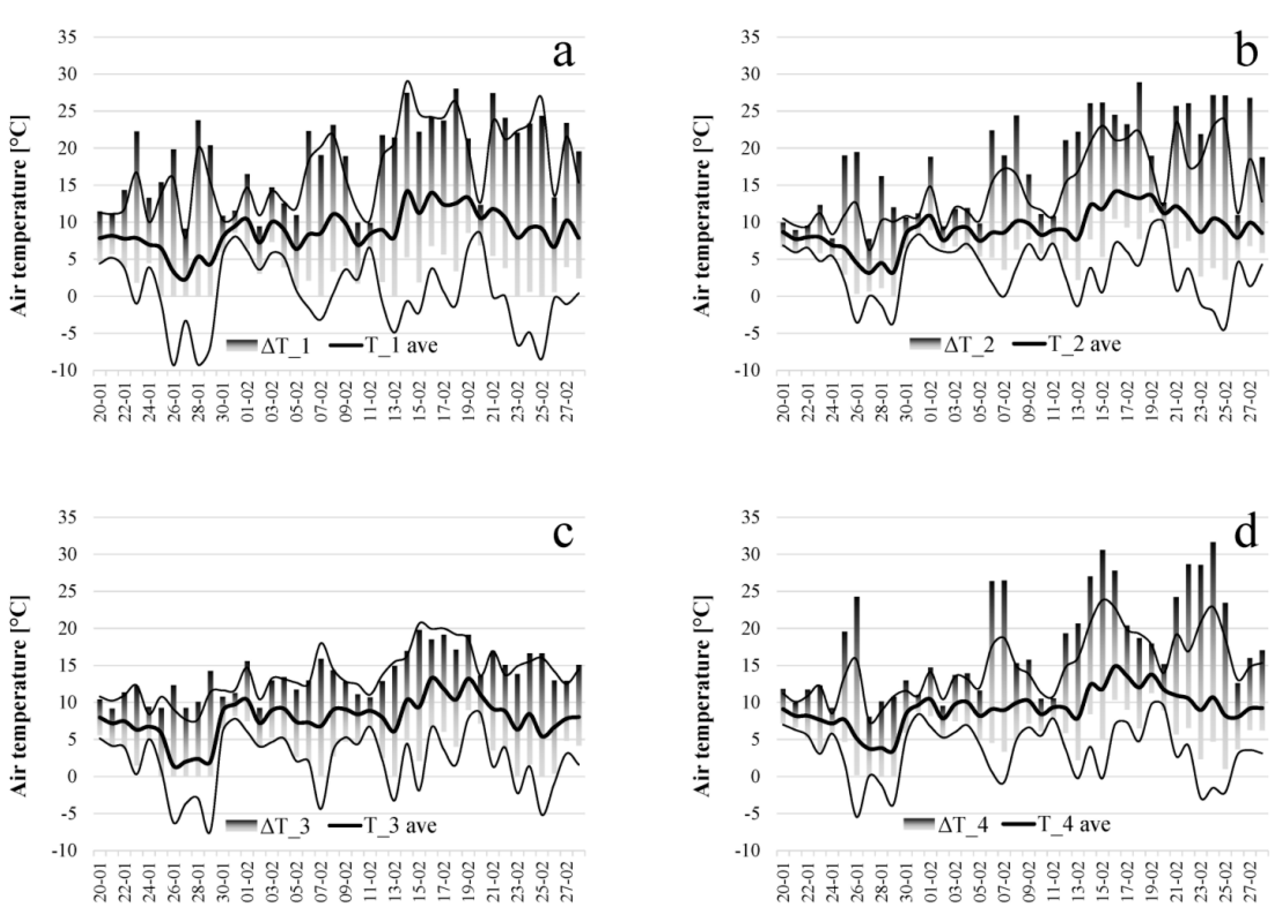
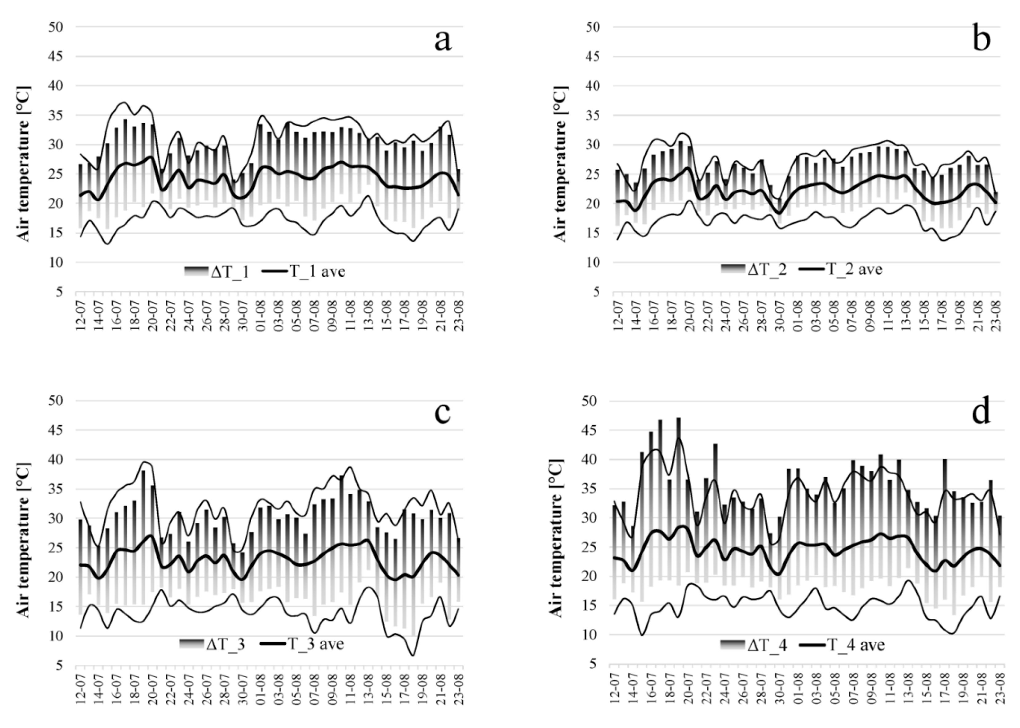
4.1. Continuous Monitoring

The monitored air temperature (T) and air relative humidity (RH) values were analyzed to describe the rural, suburban, and urban local microclimate. In addition, data of global solar radiation, wind speed, and wind direction were also observed in the suburban and urban areas. Nevertheless, the study is mainly focused on the analysis and comparison of the outdoor air temperature values available in the all investigated areas. Each environmental parameter measured through the monitoring setup described in Section 2.2 was compared with observations derived from official weather stations located in Umbria in order to validate the measurements.

The in-field monitoring has been carried out during the following periods:

-

winter, 20 January–30 April 2014;

-

summer, 12 July–23 August 2014.

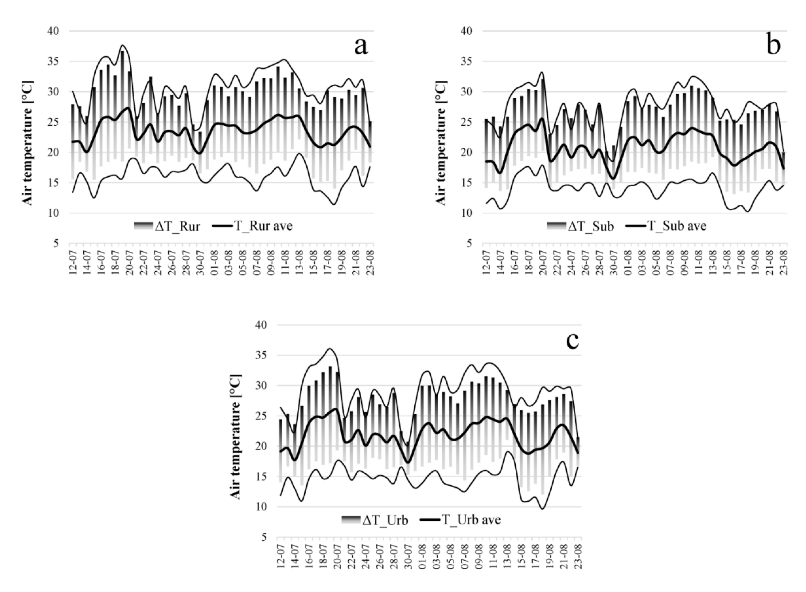
4.1.1. Air Temperature

The air temperature data measured by the four hygrothermal sensors positioned close to Lake Trasimeno shore are shown in Figure 4 and Figure 5 for two months in winter (January and February, 2014) and in summer (July and August, 2014), respectively. In particular, Figure 4 and Figure 5 show daily values of the minimum, maximum and average air temperature, and standard deviation for each measurement spot, i.e., 1, 2, 3, and 4. More in detail, the continuous upper and lower bands represent the standard deviation, while the thick central continuous band indicates the average outdoor air temperature.

While the average air temperature profiles measured in the four rural measurement spots are quite mutually consistent, significantly different peak temperatures are detected due to different local boundary phenomena of each area both in winter and summer. In fact, the air temperature is widely influenced by the thermal condition of the surrounding surfaces. More in detail, measurement spot no. 2 is characterized by slightly lower average and maximum air temperatures in summer, due to the higher presence of vegetation and low urbanization level of the area compared to the other measurement spots (see Table 1). Furthermore, in the measurement spot no. 4, located on the West side of the lake, the maximum air temperatures overcome 35 °C on most days of summer and sometimes exceed 45 °C, whereas air temperatures at measurement spot no. 2, located on the East side, barely reach 30 °C. This discrepancy is mainly due to (i) the different vegetation concentration and (ii) the strong wind coming from the West which generates the daytime cooling of the East shore of the lake. A correlation analysis among the air temperatures measured around Lake Trasimeno both in winter and summer is also carried out in order to quantify the consistency of the data derived from the four rural measurement spots. The results of the analysis are presented in Table 5.

Figure 4. Daily profiles of air temperature for the four measurement spots in winter (from 20 January to 27 February): (a) Tuoro (spot 1); (b) Torricella (spot 2); (c) Mirabella (spot 3); and (d) Castiglione del Lago (spot 4).

Figure 4. Daily profiles of air temperature for the four measurement spots in winter (from 20 January to 27 February): (a) Tuoro (spot 1); (b) Torricella (spot 2); (c) Mirabella (spot 3); and (d) Castiglione del Lago (spot 4).

Figure 5. Daily profiles of air temperature for the four measurement spots in summer (from 12 July to 23 August): (a) Tuoro (spot 1); (b) Torricella (spot 2); (c) Mirabella (spot 3); and (d) Castiglione del Lago (spot 4).

Figure 5. Daily profiles of air temperature for the four measurement spots in summer (from 12 July to 23 August): (a) Tuoro (spot 1); (b) Torricella (spot 2); (c) Mirabella (spot 3); and (d) Castiglione del Lago (spot 4).

Table 5. Correlation matrix among the average air temperature values measured in the four measurement spots around the lake.

	T_1	T_2	T_3	T_4
T_1	1	0.75	0.82	0.77
T_2	0.75	1	0.91	0.94
T_3	0.82	0.91	1	0.94
T_4	0.77	0.94	0.94	1

Table 5. Correlation matrix among the average air temperature values measured in the four measurement spots around the lake.

	T_1	T_2	T_3	T_4
T_1	1	0.75	0.82	0.77
T_2	0.75	1	0.91	0.94
T_3	0.82	0.91	1	0.94
T_4	0.77	0.94	0.94	1

The strong and positive correlation between the results (Pearson coefficient always >75%) allows to calculate the air temperature of Lake Trasimeno’s rural area as the average of the values measured by the sensors located in different positions of the same area affected by the lake presence. Additionally, the correlation matrix among the air temperatures of the rural, suburban, and urban area is presented in Table 6.

Table 6. Correlation matrix among the average air temperature values related to the rural, suburban, and urban areas.

	T_Rur	T_Sub	T_Urb
T_Rur	1	0.86	0.93
T_Sub	0.86	1	0.95
T_Urb	0.93	0.95	1

Table 6. Correlation matrix among the average air temperature values related to the rural, suburban, and urban areas.

	T_Rur	T_Sub	T_Urb
T_Rur	1	0.86	0.93
T_Sub	0.86	1	0.95
T_Urb	0.93	0.95	1

Strong and positive correlations also among the three areas (Pearson correlation coefficient always higher than 86%) are detected, both in winter and summer. The three assessed microclimates are consistent since the investigated areas are nearby (<30 km).

Figure 6 and Figure 7 show the same graphs of Figure 4 and Figure 5, but with the air temperature values measured in the rural, suburban, and urban areas for selected days of winter (January and February) and summer (July and August), respectively. Additionally, the average monthly air temperatures and the corresponded standard deviations of the three areas are summarized in Table 7.

Figure 6. Air temperature profiles for (a) rural, (b) suburban, and (c) urban area in winter (from 20 January to 27 February).

Figure 6. Air temperature profiles for (a) rural, (b) suburban, and (c) urban area in winter (from 20 January to 27 February).

Figure 7. Air temperature profiles for (a) rural; (b) suburban; and (c) urban area in summer (from 12 July to 23 August).

Figure 7. Air temperature profiles for (a) rural; (b) suburban; and (c) urban area in summer (from 12 July to 23 August).

Table 7. Average monthly air temperature with his standard deviation for the rural, suburban, and urban areas.

	T_Rur [°C]	T_Sub [°C]	T_Urb [°C]
January	6.4 ± 3.2	4.7 ± 2.5	5.6 ± 3.0
February	9.7 ± 4.0	7.7 ± 2.5	8.7 ± 3.2
March	11.1 ± 5.4	8.9 ± 4.1	9.8 ± 4.2
April	14.6 ± 5.2	11.8 ± 3.8	12.8 ± 3.9
July	23.2 ± 4.2	20.3 ± 4.1	21.5 ± 4.3
August	23.7 ± 4.3	21.1 ± 4.1	22.1 ± 4.4

Table 7. Average monthly air temperature with his standard deviation for the rural, suburban, and urban areas.

	T_Rur [°C]	T_Sub [°C]	T_Urb [°C]
January	6.4 ± 3.2	4.7 ± 2.5	5.6 ± 3.0
February	9.7 ± 4.0	7.7 ± 2.5	8.7 ± 3.2
March	11.1 ± 5.4	8.9 ± 4.1	9.8 ± 4.2
April	14.6 ± 5.2	11.8 ± 3.8	12.8 ± 3.9
July	23.2 ± 4.2	20.3 ± 4.1	21.5 ± 4.3
August	23.7 ± 4.3	21.1 ± 4.1	22.1 ± 4.4

The readings from the rural area show higher average daily and monthly air temperatures, as well as higher daily temperature fluctuations than the urban and suburban locations both in winter and summer. Differences in average monthly air temperature of about 1 °C–2 °C are found between the rural area and the other two investigated areas during the whole monitored period.

Figure 8 and Figure 9 summarize the trend of the global solar radiation measured by the urban meteorological station and the air temperature profiles of the average monthly day for the rural, suburban, and urban area in winter (from January to April) and summer conditions (in July and August), respectively. In addition, the mean daily and nightly air temperatures are listed in Table 8 and Table 9 for the winter and summer monitored months, respectively [41].

Figure 8. Winter profiles of the global solar radiation (urban station) and air temperature for rural, suburban, and urban areas in the average monthly day: (a) January; (b) February; (c) March; and (d) April.

Figure 8. Winter profiles of the global solar radiation (urban station) and air temperature for rural, suburban, and urban areas in the average monthly day: (a) January; (b) February; (c) March; and (d) April.

Figure 9. Summer profiles of the global solar radiation (urban station) and air temperature for rural, suburban, and urban areas in the average monthly day: (a) July and (b) August.

Figure 9. Summer profiles of the global solar radiation (urban station) and air temperature for rural, suburban, and urban areas in the average monthly day: (a) July and (b) August.

As previously mentioned, the rural microclimate is characterized by the highest average air temperatures, and by higher daily temperature fluctuations compared to the urban and suburban areas, both in winter and summer (Figure 8 and Figure 9). Furthermore, the rural area presents the highest night temperatures, especially in summer conditions. This is probably not due to the effect of the lake presence, but rather to the position of the sensors, which are situated at lower height above the ground compared to both the urban and suburban weather stations. This configuration makes the sensors in the rural area more affected by thermal exchanges of the surrounding environment. Additionally, the higher rural air temperature compared to the urban area is due also to the average urbanization level and the moderate vegetation presence of the selected urban area, which make it not affected by the urban heat island phenomenon.

The suburban area presents the lowest profiles of air temperature due to the low urbanization, the rich vegetation, and the highest altitude compared to both the rural and urban areas. In the suburban configuration, the altitude is the main parameter affecting the temperature reduction. Additionally, the difference between the rural area and the suburban/urban areas in terms of maximum air temperature in the average monthly day is lower in winter/summer months compared to milder months, i.e., March and April. In January, the effect of the solar radiation on the air temperature is reduced because of cloudy weather and the low intensity of the incident solar radiation. Additionally, lower time lags between the rural area and the urban and suburban area are detected in winter compared to summer months.

Finally, the air temperature differences between the rural area and the two other monitored areas are more evident during the day rather than during the night (Table 8 and Table 9).

Table 8. Main daily-nightly air temperature for the rural, suburban, and urban area (January–April).

	Average daily Air Temperature [°C] (7:00 a.m.–9:00 p.m.)			Average Nightly Air Temperature [°C] (10:00 p.m.–6.00 a.m.)
	Max	Ave	Min	Max	Ave	Min
T_Rur	18.4	13.3	6.3	12.5	7.8	1.9
T_Sub	14.8	10.2	4.3	11.7	7.0	2.0
T_Urb	16.0	11.2	5.0	12.9	7.7	1.8

Table 8. Main daily-nightly air temperature for the rural, suburban, and urban area (January–April).

	Average daily Air Temperature [°C] (7:00 a.m.–9:00 p.m.)			Average Nightly Air Temperature [°C] (10:00 p.m.–6.00 a.m.)
	Max	Ave	Min	Max	Ave	Min
T_Rur	18.4	13.3	6.3	12.5	7.8	1.9
T_Sub	14.8	10.2	4.3	11.7	7.0	2.0
T_Urb	16.0	11.2	5.0	12.9	7.7	1.8

Table 9. Main daily-nightly air temperature for the rural, suburban, and urban area (July–August).

	Average Daily Air Temperature [°C] (7:00 a.m.–9:00 p.m.)			Average Nightly Air Temperature [°C] (10:00 p.m.–6.00 a.m.)
	Max	Ave	Min	Max	Ave	Min
T_Rur	30.5	25.6	19.9	23.8	20.0	16.1
T_Sub	27.8	22.6	15.8	21.2	17.5	13.9
T_Urb	28.9	23.8	17.3	23.3	18.5	14.2

Table 9. Main daily-nightly air temperature for the rural, suburban, and urban area (July–August).

	Average Daily Air Temperature [°C] (7:00 a.m.–9:00 p.m.)			Average Nightly Air Temperature [°C] (10:00 p.m.–6.00 a.m.)
	Max	Ave	Min	Max	Ave	Min
T_Rur	30.5	25.6	19.9	23.8	20.0	16.1
T_Sub	27.8	22.6	15.8	21.2	17.5	13.9
T_Urb	28.9	23.8	17.3	23.3	18.5	14.2

From the comparison of the air temperature values among the rural, suburban, and urban area, it is evident that the monitored areas are characterized by different local microclimates and that the air temperature differences are significant, both in winter and summer. In particular, an increase of about 3.1 °C and 2.1 °C of the average daily air temperature is detected in winter in the rural area compared to the suburban and urban areas, respectively. On the contrary, during summer, the average daily air temperatures in the rural area are detected to be about 3.0 °C and 1.8 °C higher than the suburban and urban areas, respectively.

4.1.2. Air Relative Humidity

The measured air relative humidity values were briefly analyzed on a monthly basis. The monthly average air relative humidity values for the rural, suburban, and urban areas are listed in Table 10.

The highest values of air relative humidity are recorded in the rural area, due to the proximity of Lake Trasimeno.

Table 10. Monthly average relative humidity of the rural, suburban, and urban area.

	RH_Rur [%]	RH_Sub [%]	RH_Urb [%]
January	92	85	89
February	86	74	83
March	75	73	68
April	76	74	70
July	72	53	70
August	71	55	65

Table 10. Monthly average relative humidity of the rural, suburban, and urban area.

	RH_Rur [%]	RH_Sub [%]	RH_Urb [%]
January	92	85	89
February	86	74	83
March	75	73	68
April	76	74	70
July	72	53	70
August	71	55	65

4.1.3. Wind Speed and Wind Direction

The wind measured by the urban meteorological station during the investigated period comes mainly from the North direction with an average speed of 1.8 m/s. This is due to the presence of the Corciano hill, which deflects the wind along the North–South axis. When the wind comes from the lake, i.e., from Northwest and West directions, the average air temperature recorded in the urban area is 10.8 °C in winter and 22.1 °C in summer. These values are higher compared to the air temperature values of 9.8 °C and 17.8 °C measured in winter and summer, respectively, when the wind comes from all the other directions. This result confirms that the lake is able to mitigate the local urban microclimate by generating an air temperature increase both in winter and summer. However, the mitigation effect of Lake Trasimeno on the urban and suburban microclimates is not so evident from the analysis, especially in summer, because of the wind regime of the investigated region. In fact, a predominant northerly wind, which is not influenced by the lake presence, is observed in the urban area.

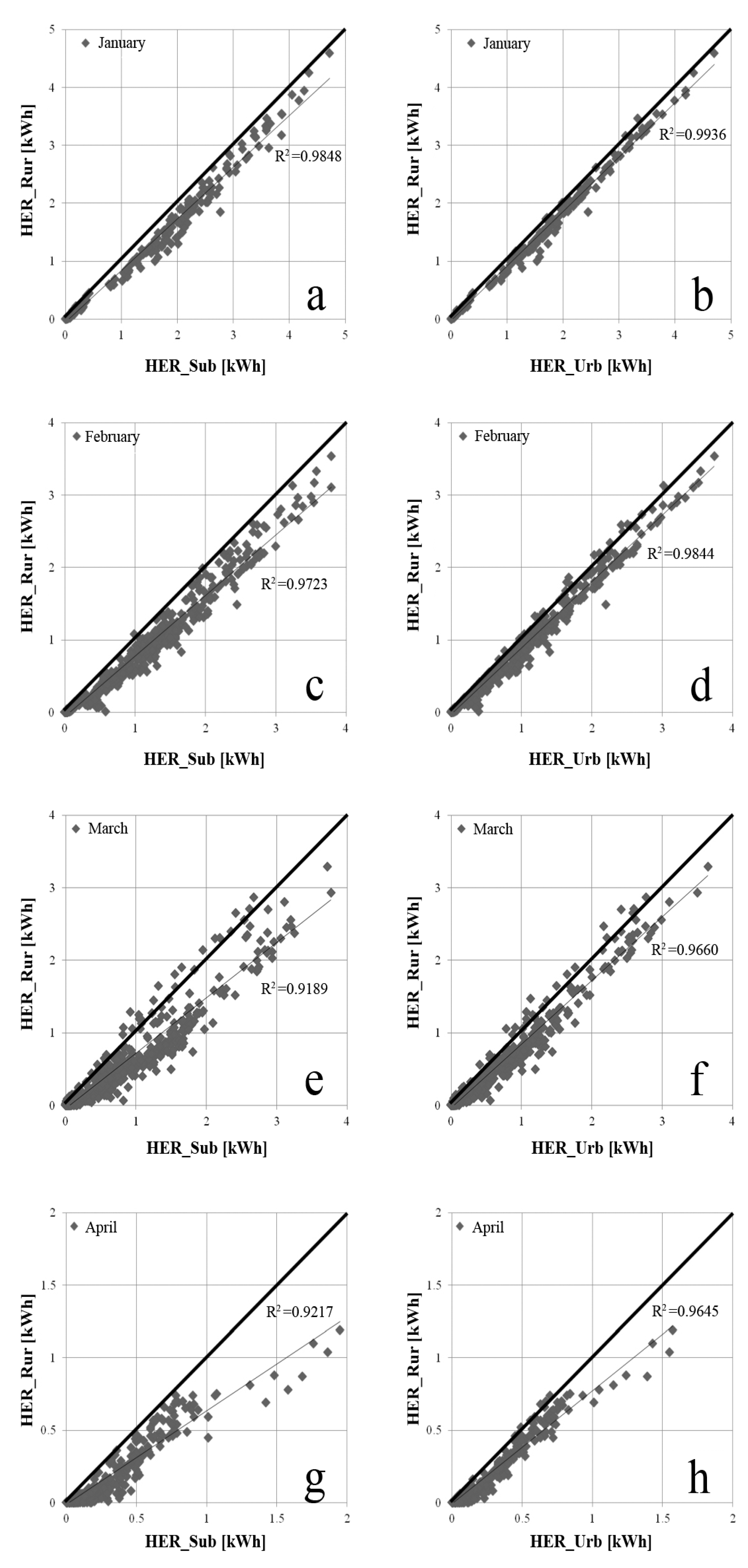
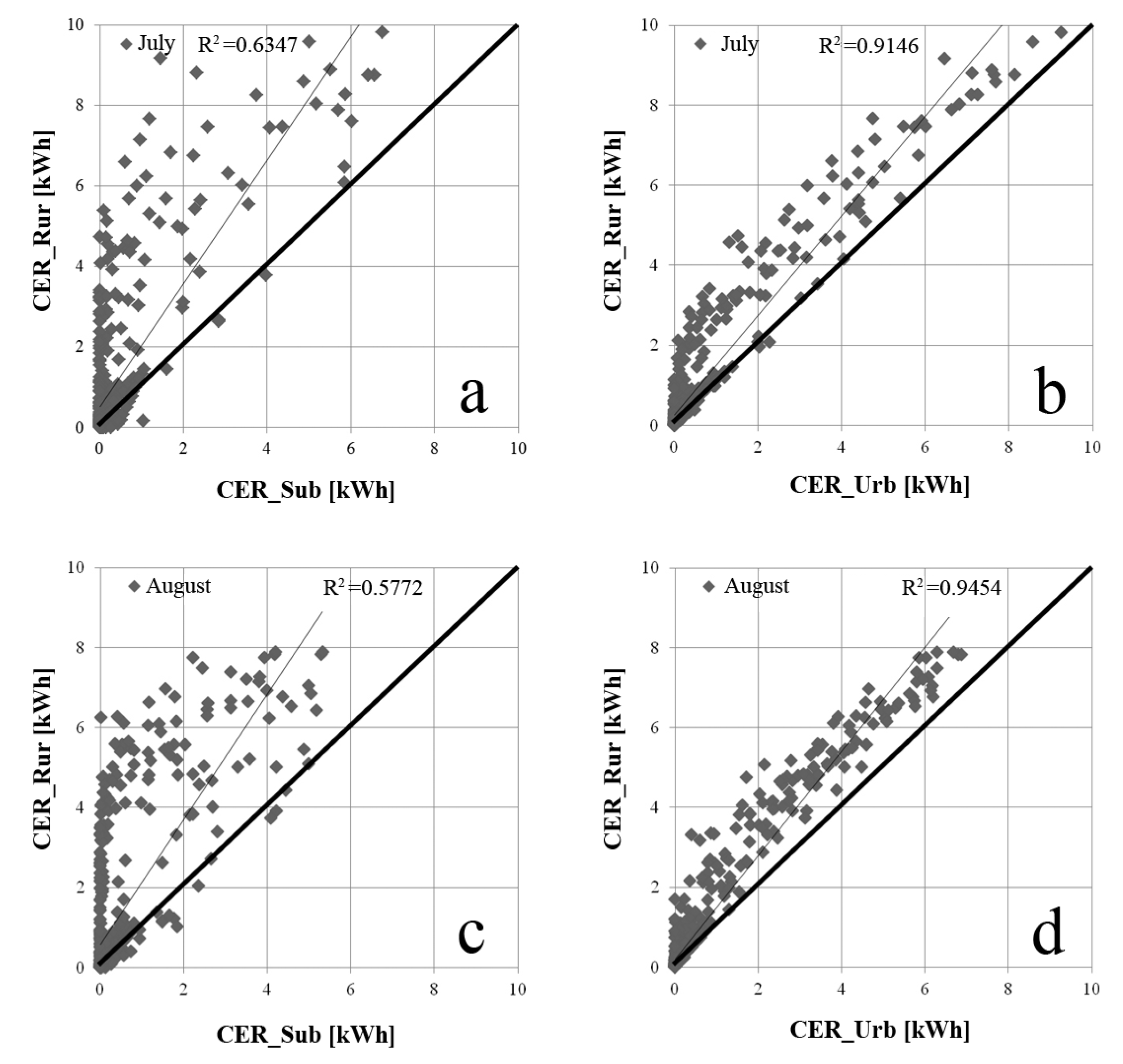
4.2. Building Energy Requirement

This section presents the results concerning the impact of microclimate variations on building energy requirement. The differences in terms of building energy requirement for heating and cooling are discussed with reference to the three considered building locations, i.e., rural, suburban, and urban areas, characterized by different microclimate boundary conditions.

First, the degree hours method is applied in order to qualitatively estimate the effect of local microclimate variations on buildings’ energy demand.

Finally, the dynamic energy simulation of a reference residential building is carried out, and the three different microclimate scenarios are analyzed in order to compare buildings energy requirement.

Each analysis is focused on the comparison between the rural area, affected by the lake presence, and the other two monitored locations, i.e., urban and suburban areas.

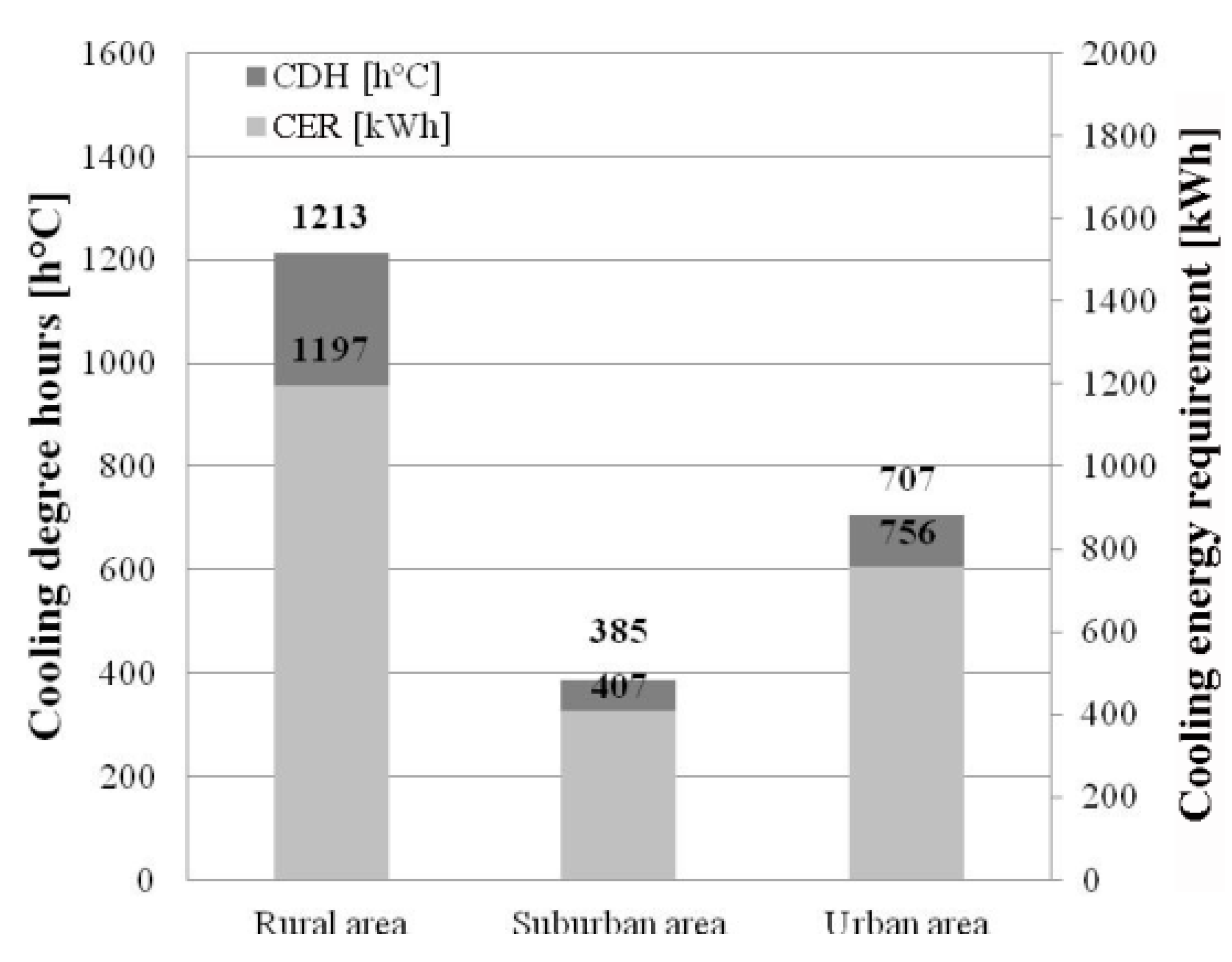
4.2.1. Degree Hour Method

As mentioned in Section 2.2, the HDH and CDH indexes are calculated as differences between outdoor air temperatures below/above the reference temperature, and the reference temperature itself. Therefore, both climate and building information are taken into account within this method. Different HDH and CDH values are obtained from the measured hourly mean temperatures for the three case study areas. The HDH indexes are equal to 11,486 h°C, 15,223 h°C, and 13,283 h°C for the rural, suburban, and urban area, respectively. For the calculation of the HDHs, the duration of the monitored period is equal to 2424 h (from 20 January to 30 April). The CDH indexes are equal to 1213 h°C, 385 h°C, and 707 h°C for the rural, suburban, and urban area, respectively. For the calculation of the CDHs, the duration of the monitored period is equal to 1032 h (from 12 July to 23 August).

The results suggest that different heating and cooling energy requirements correspond to the widely different outdoor air temperatures and local peculiar conditions of the three areas cannot be neglected both in winter and summer. In particular, buildings situated in the area close to Lake Trasimeno, i.e., rural area, need less heating than the others during the winter season. On the contrary, in summer conditions buildings situated in the rural area need more cooling than the others. This is motivated by the fact that the effect of Lake Trasimeno presence is not enough strong to mitigate in summer conditions also because of the peculiar wind regime. More in details, HDH indexes reduced of 14% and 25% are calculated for the rural area compared to the urban and suburban area, respectively. On the contrary, an increase of about 72% and 215% are found for the CDH indexes of the rural area compared to the urban and suburban area, respectively.

4.2.2. Dynamic Simulation

The results of the dynamic simulation are discussed in this section. In particular, the heating energy requirement (HER) and the cooling energy requirement (CER) of a residential building are here presented for the winter and summer monitored months and for the three assessed scenarios, i.e., rural, urban, and suburban area. The following analysis is referred to the same reference building characterized by its own energy performance. In this study, the different energy requirement depends only to the different local climate conditions, without being affected by differential building performance and further characteristics.

Figure 10 and Figure 11 show the comparison between the hourly energy requirement of the reference building for the rural area and the other two areas in winter and summer, respectively.

Figure 10. Comparison of the reference building HER between the rural area and both the suburban (a,c,e,g) and urban area (b,d,f,h) in the winter monitored period: (a,b) January; (c,d) February; (e,f) March; and (g,h) April.

Figure 10. Comparison of the reference building HER between the rural area and both the suburban (a,c,e,g) and urban area (b,d,f,h) in the winter monitored period: (a,b) January; (c,d) February; (e,f) March; and (g,h) April.

Figure 11. Comparison of the reference building CER between the rural area and both the suburban (a,c) and urban (b,d) area during the summer monitored period: (a,b) July and (c,d) August.

Figure 11. Comparison of the reference building CER between the rural area and both the suburban (a,c) and urban (b,d) area during the summer monitored period: (a,b) July and (c,d) August.

The winter analysis of the building energy requirement, in terms of primary energy for heating, shows lower consumptions in the rural area compared to the other two microclimates, i.e., suburban and urban areas, as shown in Figure 10. This means that during the monitored winter the rural microclimate had the lowest heating requirements. In the colder winter months the differences in heating energy requirement between the rural area and both the suburban and urban areas are reduced. While moving towards warmer winter months, when the HER is lower, such differences become more significant.

The greatest differences are detected between the rural and suburban areas compared to the rural and urban areas. Additionally, the HER values dispersion is lower in the case of the rural/urban area comparison with respect to the rural/suburban area comparison.

The summer analysis of the building energy requirement, in terms of primary energy for cooling, shows higher consumptions in the rural microclimate, followed by the urban and suburban scenarios, respectively, as shown in Figure 11. In particular, the CER is very low for most of the days, especially for the suburban area. Even in summer conditions greater differences are detected between the rural and suburban areas compared to differences between the rural and urban areas. Additionally, the CER values scattering is lower in the case of rural/urban area comparison rather than in the case of rural/suburban area comparison. Such phenomenon is more evident in summer than in winter.

Finally, a heating energy saving of 14% and 25% is detected for the rural area compared to the urban and suburban areas, respectively. Such values are consistent with the heating degree hours percentage previously calculated (see Section 4.2.1). Therefore, while usually the energy requirements for a specific period and location are predicted by calculating the degree hour for the same period and location, in this specific case study it is possible to predict the HERs of buildings located in the rural area by only knowing the HDHs of the suburban/urban area.

During summer, a cooling energy penalty of about 58% and 194% is found for the rural area compared to the urban and suburban areas, respectively. Different percentages, i.e., 78% and 215% compared to the urban and suburban areas, respectively, are found for the CDHs. This result is mainly due to the very low calculated cooling energy requirement for both the suburban and urban area. This implies that, for this case study, the degree hours method does not represent a good method to estimate the relative percentages of building cooling energy requirement in the rural area starting from the CDH values of the suburban or urban area. In addition, such method considers only the linear dependence between cooling energy requirement and sensible cooling load, by ignoring latent loads, which become more significant with higher outdoor temperatures.

The dynamic simulation of the reference building energy requirement in the three assessed scenarios is performed without taking into account the latent loads. With reference to this specific case study, it is necessary to know the CDH values of the rural area in order to predict the CERs of buildings located in that same area.

The results in terms of heating and cooling degree hours compared to the simulated energy requirements of the rural, suburban, and urban areas are presented in Figure 12 and Figure 13 for winter and summer monitored months, respectively.

Figure 12. Amount of the HDHs and HER for the rural, suburban, and urban area from January to April.

Figure 12. Amount of the HDHs and HER for the rural, suburban, and urban area from January to April.

Figure 13. Amount of the CDHs and CER for the rural, suburban, and urban area in July and August.

Figure 13. Amount of the CDHs and CER for the rural, suburban, and urban area in July and August.

As previously mentioned, differences in the energy requirements of buildings located in areas characterized by different local microclimates are detected. In particular, the rural area shows the lowest HER and the highest CER with respect to the other two case study areas.

5. Conclusions

In this paper, the impact of different local climate conditions on the energy performance of buildings located in different locations within the same province district is evaluated. In particular, the analysis of how local climates, and consequently building energy requirements, are affected by the proximity of a huge lake, i.e., Lake Trasimeno in central Italy, is performed. To this aim, the in-field continuous monitoring of the main environmental parameters of a rural, suburban, and urban area of the same climate zone within the maximum aerial distance of 20 kilometers, is performed during winter and summer conditions.

Coupled degree hour method and numerical analysis are applied to investigate the impact of lake proximity on the energy requirement of surrounding buildings for heating and cooling. In particular, a reference residential building is simulated in three different scenarios corresponding to the three different monitored microclimates, i.e., rural, suburban, and urban microclimate.

The main results of this work confirm that the monitored areas are characterized by different local climate boundary conditions, and that the outdoor dry bulb temperature differences are non-negligible both in winter and summer. Therefore, an increase of about 3.1 °C and 2.1 °C of the average daily air temperature is detected in winter in the rural area compared to the suburban and urban areas, respectively. On the contrary, during the monitored summer months the air temperatures in the rural area are detected to be about 3.0 °C and 1.8 °C higher than the suburban and urban areas, respectively. Consistently with the air temperature results, the air relative humidity is detected to be higher in the rural area. Additionally, differences in the energy requirement of buildings located in areas characterized by different local microclimates are detected.

The degree hours analysis shows lower HDHs and higher CDHs for the rural area with respect to the two other case study areas. In particular, a decrease of 14% and 25% in the HDHs and an increase of 78% and 215% in the CDHs are found for the rural area compared to the suburban and urban microclimates, respectively.

The dynamic simulation of the reference building energy demand in the rural area shows heating consumptions of about 14% and 25% lower than the suburban and urban microclimate scenarios, respectively. Furthermore, relatively small differences in heating energy requirement between the rural area and both the suburban and urban areas are detected. The summer analysis of the building energy requirement in terms of primary energy for cooling shows an increase of 58% and 194% for the rural area compared to the suburban and urban areas, respectively. Greater differences are detected between the rural and suburban area compared to the rural and urban areas differences. Additionally, the dispersion of cooling energy requirement values is lower in the case of rural/urban area comparison rather than in the case of rural/suburban area comparison.

According to these results, this research showed how it is always necessary to provide tailored and measured weather data, able to take into account local microclimate phenomena, while predicting building thermal-energy performance, even where there are no dense urban centers affecting local mesoclimate conditions by means, for instance, of urban heat island phenomena.

6. Limitations and Future Developments

The main limit of the present experimental campaign is represented by the fact that complete dedicated weather stations were available for only two of the case study monitored areas, i.e., urban and suburban areas. Therefore, climate data for the rural area were provided by dedicated hygrothermal sensors with data loggers positioned in the proximity of Lake Trasimeno. Future work will concern more detailed local climate analyses through continuous monitoring of additional environmental parameters in the areas around the lake. In particular, both the wind and air relative humidity will be continuously monitored to better investigate the effect of such parameters on local microclimate boundaries and, consequently, on building thermal-energy performance.

Finally, the separate effect of additional environmental boundaries i.e., altitude, vegetation, and urbanization level, on local microclimate and building energy demand will be investigated. The different envelope configurations and materials of case study buildings [42] will be taken into account.

References

1. De Wilde, P.; Coley, D. The implications of a changing climate for buildings. Build. Environ. 2012, 55, 1–7. [Google Scholar] [CrossRef] [Green Version]
2. Summerfield, A.J.; Lowe, R. Challenges and future directions for energy and buildings research. Build. Res. Inf. 2012, 40, 391–400. [Google Scholar] [CrossRef]
3. Simmonds, I.; Keay, K. Weekly cycle of meteorological variation in Melbourne and the role of pollution and anthropogenic heat release. Atmos. Environ. 1997, 31, 1589–1603. [Google Scholar] [CrossRef]
4. Kanda, M. Progress in Urban Meteorology: A review. J. Meteorol. Soc. Jpn. 2007, 85, 363–383. [Google Scholar] [CrossRef]
5. Flagg, D.D.; Taylor, P.A. Sensitivity of mesoscale model urban boundary layer meteorology to the scale of urban representation. Atmos. Chem. Phys. 2011, 6, 2951–2972. [Google Scholar] [CrossRef] [Green Version]
6. Bevilacqua, P.; Coma, J.; Pérez, G.; Chocarro, C.; Juárez, A.; Solé, C.; de Simone, M.; Cabeza, L.F. Plant cover and floristic composition effect on thermal behaviour of extensive green roofs. Build. Environ. 2015, 92, 305–316. [Google Scholar] [CrossRef]
7. Salata, F.; Golasi, I.; Vollaro, A.D.L.; Vollaro, R.D.L. How high albedo and traditional buildings’ materials and vegetation affect the quality of urban microclimate. A case study. Energy Build. 2015, 99, 32–49. [Google Scholar] [CrossRef]
8. Susorova, I.; Azimi, P.; Stephens, B. The effects of climbing vegetation on the local microclimate, thermal performance, and air infiltration of four building facade orientations. Build. Environ. 2014, 76, 113–124. [Google Scholar] [CrossRef]
9. Tao, H.; Fraedrich, K.; Menz, C.; Zhai, J. Trends in extreme temperature indices in the Poyang Lake Basin, China. Stoch. Environ. Res. Risk Assess. 2014, 28, 1543–1553. [Google Scholar] [CrossRef]
10. Chen, Z.; Zhao, L.; Meng, Q.; Wang, C.; Zhai, Y.; Wang, F. Field measurements on microclimate in residential community in Guangzhou, China. Front. Archit. Civil Eng. China 2009, 3, 462–468. [Google Scholar] [CrossRef]
11. Long, Z.; Perrie, W.; Gyakum, J.; Caya, D.; Laprise, R. Northern lake impacts on local seasonal climate. J. Hydrometeorol. 2007, 6, 881–896. [Google Scholar] [CrossRef]
12. Wuebbles, D.J.; Hayhoe, K.; Parzen, J. Introduction: Assessing the effects of climate change on Chicago and the Great Lakes. J. Great Lakes Res. 2010, 36, 1–6. [Google Scholar] [CrossRef]
13. Pisello, A.L.; Piselli, C.; Cotana, F. Thermal-physics and energy performance of an innovative green roof system: The Cool-Green Roof. Sol. Energy 2015, 116, 337–356. [Google Scholar] [CrossRef]
14. Han, Y.Q.; Taylor, J.E.; Pisello, A.L. Toward mitigating urban heat island effects: Investigating the thermal-energy impact of bio-inspired retro-reflective building envelopes in dense urban settings. Energy Build. 2015, 102, 308–389. [Google Scholar] [CrossRef]
15. Santamouris, M. On the energy impact of urban heat island and global warming on buildings. Energy Build. 2014, 82, 100–113. [Google Scholar] [CrossRef]
16. Sørensen, L.S. Heat transmission coefficient measurements in buildings utilizing a heat loss measuring device. Sustainability 2013, 5, 3601–3614. [Google Scholar] [CrossRef]
17. Santamouris, M.; Papanikolaou, N.; Nivada, I.; Koronakis, I.; Georgakis, C.; Argiriou, A.; Assimakopoulos, D.N. On the impact of urban climate on the energy consumption of buildings. Sol. Energy 2001, 70, 201–216. [Google Scholar] [CrossRef]
18. Chappells, H.; Shove, E. Debating the future of comfort: Environmental sustainability, energy consumption and the indoor environment. Build. Res. Inf. 2005, 33, 32–40. [Google Scholar] [CrossRef]
19. Wagner, K. Generation of a tropically adapted energy performance certificate for residential buildings. Sustainability 2014, 6, 8415–8431. [Google Scholar] [CrossRef]
20. Theophilou, M.K.; Serghides, D. Heat island effect for Nicosia, Cyprus. Adv. Build. Energy Res. 2014, 1, 63–73. [Google Scholar] [CrossRef]
21. Cartalis, C.; Synodinou, A.; Tsangrassoulis, A.; Santamouris, M. Modifications in energy demand in urban area as a result of climate changes: An assessment for the southeast Mediterranean region. Energy Convers. Manag. 2001, 42, 1647–1656. [Google Scholar] [CrossRef]
22. Argiriou, A.; Lykoudis, S.; Kontoyiannidis, S.; Balaras, C.A.; Asimakopoulos, D.; Petrakis, M.; Kassomenos, P. Comparison of methodologies for TMY generation using 20 years data for Athens, Greece. Solar Energy 1999, 66, 33–45. [Google Scholar] [CrossRef]
23. Cheong, C.H.; Kim, T.; Leigh, S.-B. Thermal and daylighting performance of energy-efficient windows in highly glazed residential buildings: Case study in Korea. Sustainability 2014, 6, 7311–7333. [Google Scholar] [CrossRef]
24. Jentsch, M.F.; Bahaj, A.S.; James, P.A.B. Climate change future proofing of buildings-generation and assessment of building simulation weather files. Energy Build. 2008, 40, 2148–2168. [Google Scholar] [CrossRef]
25. Matzarakis, A.; Balafoutis, C. Heating degree-days over Greece as an index of energy. Int. J. Climatol. 2004, 24, 1817–1828. [Google Scholar] [CrossRef]
26. Al-Hadhrami, L.M. Comprehensive review of cooling and heating degree days characteristics over Kingdom of Saudi Arabia. Renew. Sustain. Energy Rev. 2013, 27, 305–314. [Google Scholar] [CrossRef]
27. Durmayaz, A.; Kadioglu, M.; Sen, Z. An application of the degree-hours method to estimate the residential heating energy requirement and fuel consumption in Istanbul. Energy 2000, 25, 1245–1256. [Google Scholar] [CrossRef]
28. Tselepidaki, I.; Santamouris, M.; Asimakopoulos, D.N.; Kontoyiannidis, S. On the variability of cooling degree-days in an urban environment: Applications to Athens, Greece. Energy Build. 1994, 21, 93–99. [Google Scholar] [CrossRef]
29. Crawley, D.B.; Hand, J.W.; Kummert, M.; Griffith, B.T. Contrasting the capabilities of building energy performance simulation programs. Build. Environ. 2008, 43, 661–673. [Google Scholar] [CrossRef] [Green Version]
30. Bianchi, F.; Pisello, A.L.; Baldinelli, G.; Asdrubali, F. Infrared thermography assessment of thermal bridges in building envelope: Experimental validation in a test room setup. Sustainability 2014, 6, 7107–7120. [Google Scholar] [CrossRef]
31. Battista, G.; Evangelisti, L.; Guattari, C.; Basilicata, C.; de Lieto Vollaro, R. Buildings energy efficiency: Interventions analysis under a smart cities approach. Sustainability 2014, 6, 4694–4705. [Google Scholar] [CrossRef]
32. Canto-Perello, J.; Martinez-Garcia, M.P.; Curiel-Esparza, J.; Martin-Utrillas, M. Implementing sustainability criteria for selecting a roof assembly typology in medium span buildings. Sustainability 2015, 7, 6854–6871. [Google Scholar] [CrossRef]
33. Chan, A.L.S. Developing future hourly weather files for studying the impact of climate change on building energy performance in Hong Kong. Energy Build. 2011, 43, 2860–2868. [Google Scholar] [CrossRef]
34. Papakostas, K.; Kyriakis, N. Heating and cooling degree-hours for Athens and Thessaloniki, Greece. Renew. Energy 2005, 30, 1873–1880. [Google Scholar] [CrossRef]
35. Christenson, M.; Manz, H.; Gyalistras, D. Climate warming impact on degree-days and building energy demand in Switzerland. Energy Conserv. Manag. 2006, 47, 671–686. [Google Scholar] [CrossRef]
36. Giannakopolos, C.; Hadjinicolaou, P.; Zerefos, C.; Demosthenous, G. Changing energy requirements in the Mediterranean under changing climatic conditions. Energies 2009, 2, 805–815. [Google Scholar] [CrossRef]
37. American Society of Heating, Refrigerating and Air-Conditioning Engineers. ASHRAE Handbook Fundamentals; American Society of Heating, Refrigerating and Air-Conditioning Engineers, Inc.: Atlanta, GA, USA, 2011. [Google Scholar]
38. Crawley, D.B.; Lawrie, L.K.; Winkelmann, F.C.; Buhl, W.F.; Huang, Y.J.; Pedersen, C.O.; Strand, R.K.; Liesen, R.J.; Fisher, D.E.; Witte, M.J.; et al. Energy Plus: Creating a new-generation building energy simulation program. Energy Build. 2001, 33, 319–331. [Google Scholar] [CrossRef]
39. Bianco, V.; de Rosa, M.; Scarpa, F.; Tagliafico, L.A. Analysis of energy demand in residential buildings for different climates by means of dynamic simulation. Int. J. Ambient Energy 2014. [Google Scholar] [CrossRef]
40. American Society of Heating, Refrigerating and Air-Conditioning Engineers. ANSI/ASHRAE 55-2013: Thermal Environmental Conditions for Human Occupancy; American Society of Heating, Refrigerating and Air-Conditioning Engineers: Atlanta, GA, USA, 2013. [Google Scholar]
41. Giannopoulou, K.; Livada, I.; Santamouris, M.; Saliari, M.; Assimakopoulos, M.; Caouris, Y.G. On the characteristics of the summer urban heat island in Athens, Greece. Sustain. Cities Soc. 2011, 1, 16–28. [Google Scholar] [CrossRef]
42. Asdrubali, F.; D’Alessandro, F.; Schiavoni, S. A review of unconventional sustainable building insulation materials. Sustain. Mater. Technol. 2015. [Google Scholar] [CrossRef]